Byzantine-Robust Variance-Reduced Federated Learning over Distributed Non-i.i.d. Data

Abstract

We consider the federated learning problem where data on workers are not independent and identically distributed (i.i.d.). During the learning process, an unknown number of Byzantine workers may send malicious messages to the central node, leading to remarkable learning error. Most of the Byzantine-robust methods address this issue by using robust aggregation rules to aggregate the received messages, but rely on the assumption that all the regular workers have i.i.d. data, which is not the case in many federated learning applications. In light of the significance of reducing stochastic gradient noise for mitigating the effect of Byzantine attacks, we use a resampling strategy to reduce the impact of both inner variation (that describes the sample heterogeneity on every regular worker) and outer variation (that describes the sample heterogeneity among the regular workers), along with a stochastic average gradient algorithm to gradually eliminate the inner variation. The variance-reduced messages are then aggregated with a robust geometric median operator. We prove that the proposed method reaches a neighborhood of the optimal solution at a linear convergence rate and the learning error is determined by the number of Byzantine workers. Numerical experiments corroborate the theoretical results and show that the proposed method outperforms the state-of-the-arts in the non-i.i.d. setting.

I Introduction

With the rapid increase of data volume and computing power, the past decades have witnessed the explosive development of machine learning. However, many machine learning methods require a central server or a cloud to collect data from various owners and train models in a centralized manner, leading to serious privacy concerns. To address this issue, federated learning keeps data private at their owners and carries out machine learning tasks locally [1, 2, 3, 4, 5, 6]. Every data owner (called worker thereafter) performs local computation based on its local data and sends the results (such as local models, gradients, stochastic gradients, etc) to the central server. The central server (called central node thereafter) aggregates the results received from the workers and updates the global model.

Nevertheless, the distributed nature of federated learning makes it vulnerable to attacks [4]. Due to the heterogeneity of federated learning systems, workers are not all reliable. Some workers might be malfunctioning or even adversarial, and send malicious messages to the central node. This paper considers the classical Byzantine attack model [7], where an unknown number of Byzantine workers are omniscient, collude with each other, and send arbitrary malicious messages. Moreover, the identities of Byzantine workers are unknown to the central node. Misled by the Byzantine workers, the aggregation at the central node is problematic, such that the federated learning method may converge to an unsatisfactory model or even diverge. For instance, the popular distributed stochastic gradient descent (SGD) method fails at presence of Byzantine attacks from a single worker [8].

Most of the Byzantine-robust distributed methods modify distributed SGD to handle Byzantine attacks, by replacing mean aggregation with robust aggregation at the central node [9, 10, 11]. When the data on the workers are independent and identically distributed (i.i.d.) and the local cost functions are in the same form, stochastic gradients computed at the same point are i.i.d. too. Therefore, various robust aggregation rules, such as geometric median [8], can be applied to alleviate the effect of statistically biased messages sent by Byzantine workers. Unfortunately, the data on the workers are often non-i.i.d. in federated learning applications [12, 13]. Thus, the messages sent by the regular workers are no longer i.i.d. such that handling Byzantine attacks becomes more challenging.

I-A Our contributions

In the Byzantine-robust federated learning setting, this paper considers the distributed finite-sum minimization problem when the workers have non-i.i.d. data. Our contributions are summarized as follows.

C1) In light of the significance of reducing stochastic gradient noise for mitigating the effect of Byzantine attacks, we propose a Byzantine-robust variance-reduced SGD method, using a resampling strategy to reduce the impact of both inner variation (that describes the sample heterogeneity on every regular worker) and outer variation (that describes the sample heterogeneity among the regular workers), while a stochastic average gradient algorithm (SAGA) to fully eliminate the inner variation. The variance-reduced messages are then aggregated with a robust geometric median operator.

C2) We prove that the proposed method reaches a neighborhood of the optimal solution at a linear convergence rate, and the learning error is explicitly determined by the number of Byzantine workers.

C3) We conduct numerical experiments on convex and nonconvex federated learning problems and in i.i.d. and non-i.i.d. settings. The experimental results corroborate the theoretical findings and show that the proposed method outperforms the state-of-the-arts, especially in the non-i.i.d. setting.

I-B Related works

Federated learning, in a nutshell, belongs to the category of distributed optimization, for which there are extensive works, ranging from machine learning, signal processing to system control. For example, [14] proposes a projected primal-dual method to solve the distributed constrained nonsmooth convex optimization problem. Aiming at the distributed time-varying formation problem, [15] proposes a distributed framework with the help of time-varying optimization methods. Below we focus on the related works in Byzantine-robustness of distributed algorithms, especially those handling non-i.i.d. data.

Byzantine-robust distributed machine learning has attracted much attention in recent years. In distributed SGD, the central node aggregates messages received from the workers by taking average and uses the mean as aggregated gradient direction. The mean aggregation, however, is vulnerable to Byzantine attacks. Existing Byzantine-robust distributed methods mostly extend the distributed SGD with robust aggregation rules, such as geometric median [8], normalized aggregation [16], coordinate-wise median [17], coordinate-wise trimmed mean [17], Krum [18], multi-Krum [18], Bulyan [19], to name a few. Algorithms leveraging second-order information has also be considered in [20]. Another approach is to detect and discard outliers from the received messages [21, 22, 23]. When the received stochastic gradients from the regular workers satisfy the i.i.d. assumption, the statistically different malicious messages from the Byzantine workers can be detected and discarded, or their negative effect can be alleviated by robust aggregation rules. For network anomaly detection in distributed online optimization, [24] proposes a distributed one-class support vector machine method.

Aiming at Byzantine-robustness with distributed non-i.i.d. data, [25] proposes a robust stochastic aggregation method that employs model aggregation rather than stochastic gradient aggregation. Forced by the introduced consensus constraints, the regular workers and the central node shall reach consensus on their local models, no matter the local data are i.i.d. or not. [26] also imposes asymptotic consensus between the regular workers and the central node, and proposes a Byzantine-robust proximal stochastic gradient method. [27] divides the cost functions of the workers into several clusters, such that within each cluster the i.i.d. assumption approximately holds. Then robust aggregation can be applied within each cluster. [28] introduces a resampling strategy to reduce the heterogeneity of the received messages in the non-i.i.d. setting.

In both i.i.d. and non-i.i.d. settings, variance of the messages sent by the regular workers plays a critical role to Byzantine-robustness. Larger variance means that the malicious messages are harder to distinguish. Theoretically, the variance can be classified into inner variation that describes the sample heterogeneity on every regular worker and outer variation that describes the sample heterogeneity among the regular workers. In the i.i.d. setting the inner variation often dominates, while in the non-i.i.d. setting the outer variation can be large. [29] and its extended version [30] use SAGA to correct the stochastic gradients and aggregate the corrected stochastic gradients with geometric median. It has been proven that the impact of inner variation is fully eliminated from the learning error. [31] combines stochastic variance-reduced gradient (SVRG) with robust aggregation to solve distributed non-convex problems. [32] proves that the momentum method can reduce the variance of the stochastic gradients for the regular workers relative to their norm, and is thus helpful to Byzantine-robustness. [33] also claims that applying the momentum method can reduce the variance and enhance Byzantine-robustness. The resampling strategy used in [28] is able to reduce the impact of inner and outer variations simultaneously.

The work of this paper is closely related to [30] and [28], but not a simple combination of them. First, the theme of [30] is to investigate the importance of variance reduction to Byzantine-robustness for i.i.d. data, while this work considers non-i.i.d. data. [28] studies reducing the impact of inner and outer variations by resampling, but is unable to eliminate the impact of inner variation. Second, the theoretical analysis is more difficult than that in [30] and [28] because of the entanglement of variance reduction and resampling. We will highlight the differences of our lemmas and theorems in Section IV.

II Problem Formulation and Preliminaries

Consider a federated learning system consisting of one central node and $W:=R+B$ workers, among which $R$ workers are regular and $B$ workers are Byzantine. However, the numbers and identities of Byzantine workers are unknown to the central node. During the learning process, the Byzantine workers can collude to send arbitrary malicious messages to the central node [7]. Denote the sets of regular and Byzantine workers as $\mathcal{R}$ and $\mathcal{B}$, respectively, with $R=|\mathcal{R}|$ and $B=|\mathcal{B}|$. Denote $\mathcal{W}:=\mathcal{R}\cup\mathcal{B}=\{1,\cdots,W\}$ as the set of all workers. The goal is to find an optimal solution to the finite-sum minimization problem

$$x^{*}=\arg\min_{x}f(x):=\frac{1}{R}\sum_{w\in\mathcal{R}}f_{w}(x),$$ (1)

with

$$f_{w}(x):=\frac{1}{J}\sum_{j=1}^{J}f_{w,j}(x).$$ (2)

Here $x\in\mathbb{R}^{p}$ is the optimization variable, and $f_{w}(x)$ is the local cost function of regular worker $w$ averaging the costs $f_{w,j}(x)$ of $J$ samples. The samples are not necessarily i.i.d. across the regular workers. This finite-sum minimization form arises in many federated learning applications [3].

When the Byzantine workers are absent, distributed SGD [34] is a popular method to solve (1). The update of distributed SGD is given by

$$x^{k+1}=x^{k}-\gamma\cdot\frac{1}{W}\sum_{w=1}^{W}f^{\prime}_{w,i_{w}^{k}}(x^{k}),$$ (3)

where $\gamma$ is the step size and $i_{w}^{k}$ is the sample index chosen by worker $w$ at time $k$. Upon receiving $x^{k}$ from the central node, every worker $w$ computes a stochastic gradient $f^{\prime}_{w,i_{w}^{k}}(x^{k})$ and returns it to the central node. The central node then averages the received stochastic gradients and updates $x^{k+1}$. However, distributed SGD is vulnerable to Byzantine attacks. Even there is only one Byzantine worker, it can replace the true stochastic gradient with a malicious message, such that the average at the central node becomes zero or infinitely large [9].

Geometric median. To address this issue, most of the Byzantine-robust methods aggregate the received messages with robust aggregation rules. One popular approach is geometric median [8]. To be specific, define $g_{w}^{k}$ as the message sent by worker $w$ at time $k$ to the central node, given by

$$g_{w}^{k}=\left\{\begin{aligned} &f^{\prime}_{w,i_{w}^{k}}(x^{k}),&&w\in\mathcal{R},\\ &*,&&w\in\mathcal{B}.\end{aligned}\right.$$ (4)

When $w$ is a regular worker, it sends the true stochastic gradient $f^{\prime}_{w,i_{w}^{k}}(x^{k})$. Otherwise when $w$ is a Byzantine worker, it sends an arbitrary message denoted by $*$. Upon receiving all the messages, the central node calculates the geometric median of $\{g_{w}^{k},w\in\mathcal{W}\}$, which is

$$\mathrm{geomed}\left(\{g_{w}^{k},w\in\mathcal{W}\}\right):=\arg\min_{g}\sum_{w=1}^{W}\|g-g_{w}^{k}\|_{2}.$$ (5)

Then, the central node updates $x^{k+1}$ by replacing the average in (3) with the geometric median, as

$$x^{k+1}=x^{k}-\gamma\cdot\mathrm{geomed}\left(\{g_{w}^{k},w\in\mathcal{W}\}\right).$$ (6)

It has been proved that when the regular workers have i.i.d. data, incorporating distributed SGD and geometric median allows us to tolerate Byzantine attacks when less than half of the workers are malicious, namely, $B<\frac{W}{2}$ [8]. However, when the regular workers have non-i.i.d. data, simply combining geometric median with distributed SGD is unable to defend against Byzantine attacks [25].

Why large variance hurts? To understand the importance of variance reduction to robust aggregation, we review the following concentration property of geometric median from [30, Lemma 1].

Property 1.

Let $\{z_{w},w\in\mathcal{W}\}$ be a set of random vectors. It holds when $B<\frac{W}{2}$ that

$$\mathbb{E}\|\mathrm{geomed}\left(\{z_{w},w\in\mathcal{W}\}\right)-\bar{z}\|^{2}$$ (7)

$$\leq \frac{C_{\alpha}^{2}}{R}\sum_{w\in\mathcal{R}}{\mathbb{E}\|z_{w}-\mathbb{E}z_{w}\|^{2}}+\frac{C_{\alpha}^{2}}{R}\sum_{w\in\mathcal{R}}{\|\mathbb{E}z_{w}-\bar{z}\|^{2}},$$

where $\bar{z}:=\frac{1}{R}\sum_{w\in\mathcal{R}}\mathbb{E}z_{w}$, $\alpha:=\frac{B}{W}$, $C_{\alpha}:=\frac{2-2\alpha}{1-2\alpha}$, and $\mathbb{E}$ is taken over the random vectors.

Suppose $z_{w}=g_{w}^{k}$ as defined (4), such that $z_{w}$ is the true stochastic gradient when $w$ is regular, and an arbitrary malicious message when $w$ is Byzantine. The left-hand side of (7) denotes the mean-square error of the geometric median relative to the average of the true stochastic gradients. The right-hand side of (7) contains two terms. The first term now refers to the cross-sample variance (a.k.a. inner variation), while the second term refers to the cross-worker variance (a.k.a. outer variation). When either the inner variation or the outer variation is large, the geometric median aggregation yields a poor direction that eventually leads to large learning error, as illustrated in Fig. 1. This fact motivates Byrd-SAGA [29, 30]. It has been shown in [29, 30] that SAGA effectively eliminates the inner variation, i.e., the first term at the right-hand side of (7). However, for the non-i.i.d. case, the second term at the right-hand side of (7) can be large and still deteriorate the performance of robust aggregation.

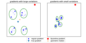
Figure 1: An illustration of the impact of inner and outer variations on geometric median under Byzantine attacks. Suppose 8 regular workers sample stochastic gradients from 4 distributions. When the variations are large, the Byzantine-free true average is far away from the geometric median under Byzantine attacks. In contrast, when the variations are small, the gap is small too.

III Algorithm Development

In light of the fact that the messages with large variance affect the robust aggregation performance, we propose to simultaneously reduce the inner and outer variations so as to achieve better performance in the non-i.i.d. setting. Specifically, we use the variance-reduced stochastic gradients at the worker side to gradually eliminate the inner variation, and use a resample-then-aggregate strategy at the central node to reduce outer variation.

Our proposed method is described as follows. At time $k$, the central node broadcasts its current variable $x^{k}$ to all the workers. Instead of sending the stochastic gradients to the central node, the regular workers send the corrected, variance-reduced stochastic gradients. To be specific, every regular worker stores the most recent stochastic gradient for every of its samples. When regular worker $w$ selects the sample index $i_{w}^{k}$ at time $k$, the corrected stochastic gradient is

$$f^{\prime}_{w,i_{w}^{k}}(x^{k})-f^{\prime}_{w,i_{w}^{k}}(\phi_{w,i_{w}^{k}}^{k})+\frac{1}{J}\sum_{j=1}^{J}f^{\prime}_{w,j}(\phi_{w,j}^{k}),$$ (8)

where

$$\phi_{w,j}^{k+1}=\left\{\begin{aligned} &\phi_{w,j}^{k},&&j\neq i_{w}^{k},\\ &x^{k},&&j=i_{w}^{k}.\end{aligned}\right.$$ (9)

That is, the stochastic gradient $f^{\prime}_{w,i_{w}^{k}}(x^{k})$ is corrected by first subtracting the previously stored stochastic gradient $f^{\prime}_{w,i_{w}^{k}}(\phi_{w,i_{w}^{k}}^{k})$ for sample $i_{w}^{k}$, and then adding the average of all the stored stochastic gradients $f^{\prime}_{w,j}(\phi_{w,j}^{k})$. At time $k$, denote $v_{w}^{k}$ as the corrected stochastic gradient if $w$ is regular and an arbitrary message $*$ if $w$ is Byzantine, given by

$$\!\!\!\!v_{w}^{k}=\left\{\begin{aligned} &f^{\prime}_{w,i_{w}^{k}}(x^{k})-f^{\prime}_{w,i_{w}^{k}}(\phi_{w,i_{w}^{k}}^{k})&&\\ &\hskip 30.00005pt+\frac{1}{J}\sum_{j=1}^{J}f^{\prime}_{w,j}(\phi_{w,j}^{k}),&&w\in\mathcal{R},\\ &*,&&w\in\mathcal{B}.\end{aligned}\right.$$ (10)

Algorithm 1 Resampling $\mathbf{RS}\left(\{v_{w}^{k},w\in\mathcal{W}\},s\right)$

Input: variance-reduced worker gradients $\{v_{w}^{k},w\in\mathcal{W}\}$, $s$

1:Initialize $\{c_{w}=0,w\in\mathcal{W}\}$

2:for $w=1,\cdots$, $W$ do

3:    for $\zeta=1,\cdots,s$ do

4:         Select $w_{\zeta}\sim\textbf{Uniform}(\{w^{\prime}|w^{\prime}\in\mathcal{W},c_{w^{\prime}}<s\})$

5:         $c_{w_{\zeta}}=c_{w_{\zeta}}+1$     

6:    Compute average $\tilde{v}_{w}^{k}=\frac{1}{s}\sum_{\zeta=1}^{s}v_{w_{\zeta}}^{k}$

7:Return $\{\tilde{v}_{w}^{k},w\in\mathcal{W}\}$

Building upon [28], we leverage a resample-then-aggregate strategy to reduce the outer variation in the non-i.i.d. case. After receiving the messages $\{v_{w}^{k},w\in\mathcal{W}\}$ from all the workers, the central node takes $W$ rounds of sampling, and uniformly at random samples $s$ messages at every round. The $W$ rounds of sampling follows sampling with $s$-replacement mechanism: when one message has been sampled for $s$ times, it will not be sampled again. At the end of each round $w$, the central node averages the $s$ sampled messages to calculate the new message $\tilde{v}_{w}^{k}$. See a summary in Algorithm 1.

We denote this resampling procedure with $s$-replacement as

$$\{\tilde{v}_{w}^{k},w\in\mathcal{W}\}=\mathbf{RS}\left(\{v_{w}^{k},w\in\mathcal{W}\},s\right).$$ (11)

Compared to the original messages $\{v_{w}^{k},w\in\mathcal{W}\}$, the new messages $\{\tilde{v}_{w}^{k},w\in\mathcal{W}\}$ have smaller variance due to the averaging step. In addition, at most $sB$ new messages are contaminated by the malicious messages $\{v_{w}^{k},w\in\mathcal{B}\}$, and the variance of uncontaminated new messages is also smaller than that of $\{v_{w}^{k},w\in\mathcal{R}\}$. Fig. 2 gives a deterministic example, showing that resampling indeed reduces the outer variation. For the stochastic case, the inner variation is reduced too.

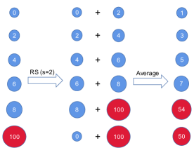
Figure 2: An illustration the variance-reducing effect of resampling, where 5 true messages (marked in blue) and 1 malicious message (marked in red) enters the resampling procedure with $s=2$. After the averaging step, at most 2 messages are contaminated. The variation of all the 6 original messages is $3860/3$, and that of all the 6 messages after resampling is $1550/3$. In addition, the variation of all the 5 original true messages is 8, and that of all the 4 uncontaminated messages after resampling is 5.

Finally, the central node updates the variable from

$$x^{k+1}=x^{k}-\gamma\cdot\mathrm{geomed}\left(\{\tilde{v}_{w}^{k},w\in\mathcal{W}\}\right).$$ (12)

See a summary of our proposed method in Algorithm 2.

Algorithm 2 Byzantine-Robust Variance-Reduced Federated Learning over Distributed Non-i.i.d. Data

central node:

1:Input $x^{0}\in\mathbb{R}^{p}$, $\gamma$, $s$. At time $k$:

2:Broadcast its current variable $x^{k}$ to all workers

3:Receive messages $\{v_{w}^{k},w\in\mathcal{W}\}$ from all workers

4:Generate $\{\tilde{v}_{w}^{k},w\in\mathcal{W}\}$ from $\{v_{w}^{k},w\in\mathcal{W}\}$ according to Algorithm 1 with parameter $s$

5:Update $x^{k+1}=x^{k}-\gamma\cdot\mathrm{geomed}\left(\{\tilde{v}_{w}^{k},w\in\mathcal{W}\}\right)$

Regular worker $w$:

1:Initialize $\{f^{\prime}_{w,j}(\phi_{w,j}^{0})=f^{\prime}_{w,j}(x^{0}),~{}j\in\{1,\cdots,J\}\}$. At time $k$:

2:Receive variable $x^{k}$ from central node

3:Compute $\bar{g}_{w}^{k}=\frac{1}{J}\sum_{j=1}^{J}f^{\prime}_{w,j}(\phi_{w,j}^{k})$.

4:Sample $i_{w}^{k}$ uniformly randomly from $j\in\{1,\cdots,J\}$

5:Update $v_{w}^{k}=f^{\prime}_{w,i_{w}^{k}}(x^{k})-f^{\prime}_{w,i_{w}^{k}}(\phi_{w,i_{w}^{k}}^{k})+\bar{g}_{w}^{k}$

6:Store stochastic gradient $f^{\prime}_{w,i_{w}^{k}}(\phi_{w,i_{w}^{k}}^{k})=f^{\prime}_{w,i_{w}^{k}}(x^{k})$

7:Send corrected stochastic gradient $v_{w}^{k}$ to central node

IV Theoretical Analysis

In this section, we theoretically analyze the performance of the proposed method, as well as investigate the effect of reducing the inner and outer variations on robust aggregation.

IV-A Assumptions

We start from introducing three assumptions on the sample costs $\{f_{w,j},w\in\mathcal{R},j=1,\cdots,J\}$.

Assumption 1.

(Strong convexity and Lipschitz continuous gradients) The function $f$ is $\mu$-strong convex and has $L$-Lipschitz continuous gradients. Namely, for any $x,y\in{\mathbb{R}}^{p}$, it holds that

$$f(y)\geq f(x)+\langle f^{\prime}(x),y-x\rangle+\frac{\mu}{2}\|y-x\|^{2},$$ (13)

and

$$\|f^{\prime}(y)-f^{\prime}(x)\|\leq L\|y-x\|.$$ (14)

Assumption 2.

(Bounded outer variation) For any $x\in{\mathbb{R}}^{p}$, the variation of the local gradients at the regular workers with respect to the global gradient is upper-bounded by

$$\frac{1}{R}\sum_{w\in\mathcal{R}}\|f^{\prime}_{w}(x)-f^{\prime}(x)\|^{2}\leq\delta^{2}.$$ (15)

Assumption 3.

(Bounded inner variation) For every regular worker $w\in\mathcal{R}$ and any $x\in{\mathbb{R}}^{p}$, the variation of its stochastic gradients with respect to its local gradient is upper-bounded by

$$\mathbb{E}\|f^{\prime}_{w,i_{w}^{k}}(x)-f^{\prime}_{w}(x)\|^{2}\leq\sigma^{2},~{}\forall w\in\mathcal{R}.$$ (16)

Here we use $\mathbb{E}$ to denote the expectation with respect to all random variables $i_{w}^{k}$.

Assumption 1 is standard for analyzing distributed learning algorithms. Assumptions 2 and 3 bound the inner variation that describes the sample heterogeneity on every regular worker and the outer variation that describes the sample heterogeneity among the regular workers, respectively. When all the samples at the regular workers are identical, both the inner variation and the outer variation are zero. When the distributed data are i.i.d. the inner variation is often larger than the outer variation, while for the non-i.i.d. case the outer variation usually dominates.

IV-B Concentration properties

Interestingly, augmented with the resampling strategy, geometric median shows better dependency on both the inner variation and the outer variation than that without resampling (as shown in Property 1). We give the following lemma.

Lemma 1.

Let $\{z_{w},w\in\mathcal{W}\}$ be a subset of random vectors distributed in a normed vector space and the random vectors in $\{z_{w},w\in\mathcal{R}\}$ are independent. Generate from $\{z_{w},w\in\mathcal{W}\}$ a new set $\{\tilde{z}_{w},w\in\mathcal{W}\}$ using the resampling strategy with $s$-replacement. It holds when $B<\frac{W}{2s}$ that

$$\mathbb{E}\|\mathrm{geomed}\left(\{\tilde{z}_{w},w\in\mathcal{W}\}\right)-\bar{z}\|^{2}$$ (17)

$$\leq \left(d+\frac{1-d}{R}\right)\frac{C_{s\alpha}^{2}}{R}\sum_{w\in\mathcal{R}}{\mathbb{E}\|z_{w}-\mathbb{E}z_{w}\|^{2}}$$

$$+\frac{dC_{s\alpha}^{2}}{R}\sum_{w\in\mathcal{R}}{\|\mathbb{E}z_{w}-\bar{z}\|^{2}},$$

where $\bar{z}:=\frac{1}{R}\sum_{w\in\mathcal{R}}\mathbb{E}z_{w}$, $\alpha:=\frac{B}{W}$, $C_{s\alpha}:=\frac{2-2s\alpha}{1-2s\alpha}$, $d:=\frac{W-1}{sW-1}$, and $\mathbb{E}$ is taken over the random vectors and the resampling process.

Comparing the bounds of mean-square errors given by (7) and (17), we observe that the coefficients change. When $s=1$, the two bounds are identical. When $s>1$, the coefficients in (17) smaller than those in (7) if $\alpha$ is sufficiently small, meaning that the inner variation and the outer variation are simultaneously reduced. The cost, however, is the capability of tolerating a smaller fraction of Byzantine workers. We will numerically depict the effect of variance reduction in Fig. 3 when discussing the main theorem.

Again, suppose $z_{w}=g_{w}^{k}$ as defined in (4). Then, the right-hand side of (17) contains two terms, one for inner variation and another for outer variation. Resampling can reduce the dependency on both the inner and outer variations, but cannot eliminate the inner variation. We shall see in the main theorem that, the unique coupling of SAGA and resampling in our proposed method is able to eliminate the inner variation, and hence leads to reduced learning error.

Remark 1. Above, we have discussed the connection between Lemma 1 and [30, Lemma 1]. Technically, to prove Lemma 1, we need to apply [28, Proposition 1] to guarantee the reduction of upper bound for the mean-square error as in (17). We also utilize the fact that the random vectors are independent to obtain a tight bound.

The intermediate result of Lemma 1 is the following lemma, which characterizes how the averaged mean-square error of a number of vectors depends on the inner and outer variations after resampling.

Lemma 2.

Let $\{z_{w},w\in\mathcal{W}\}$ be a subset of random vectors distributed in a normed vector space and the random vectors in $\{z_{w},w\in\mathcal{R}\}$ are independent. Generate from $\{z_{w},w\in\mathcal{W}\}$ a new set $\{\tilde{z}_{w},w\in\mathcal{W}\}$ using the resampling strategy with $s$-replacement. When $B<\frac{W}{s}$, there exists a set $\mathcal{R}^{\prime}\subseteq\mathcal{W}$ with at least $W-sB$ elements, such that for any $w^{\prime}\in\mathcal{R}^{\prime}$, it holds that

$$\frac{1}{|\mathcal{R^{\prime}}|}\sum_{w^{\prime}\in\mathcal{R}^{\prime}}\mathbb{E}\|\tilde{z}_{w^{\prime}}-\bar{z}\|^{2}$$ (18)

$$= \left(d+\frac{1-d}{R}\right)\frac{1}{R}\sum_{w\in\mathcal{R}}\mathbb{E}\left\|z_{w}-\mathbb{E}z_{w}\right\|^{2}$$

$$+\frac{d}{R}\sum_{w\in\mathcal{R}}\left\|\mathbb{E}z_{w}-\bar{z}\right\|^{2},$$

where $\bar{z}:=\frac{1}{R}\sum_{w\in\mathcal{R}}\mathbb{E}z_{w}$, $d:=\frac{W-1}{sW-1}$, and $\mathbb{E}$ is taken over all the randomness.

Without resampling, we have the decomposition

$$\frac{1}{R}\sum_{w\in\mathcal{R}}\mathbb{E}\|z_{w}-\bar{z}\|^{2}$$ (19)

$$= \frac{1}{R}\sum_{w\in\mathcal{R}}\mathbb{E}\left\|z_{w}-\mathbb{E}z_{w}\right\|^{2}+\frac{1}{R}\sum_{w\in\mathcal{R}}\left\|\mathbb{E}z_{w}-\bar{z}\right\|^{2}.$$

Let us compare the two equalities (18) and (19). The left-hand sides of (18) and (19) are the mean-square errors of $\{\tilde{z}_{w^{\prime}},w^{\prime}\in\mathcal{R}^{\prime}\}$ and $\{z_{w},w\in\mathcal{R}\}$ relative to $\bar{z}$, respectively. Since $d+\frac{1-d}{R}\leq 1$ and $d\leq 1$, we see that the bias of $\{\tilde{z}_{w^{\prime}},w^{\prime}\in\mathcal{R}^{\prime}\}$ to $\bar{z}$ is smaller than the bias of $\{z_{w},w\in\mathcal{R}\}$ to $\bar{z}$, showing the “variance reduction” property of resampling.

Remark 2. The proof of Lemma 2 is nontrivial. We handle the variance of resampled vectors from two aspects, namely, the mean-square error between resampled vectors and original vectors and that between original vectors and averaged vector. This enables the application of [28, Proposition 1] to the proof.

IV-C Main theorem

The following main theorem establishes the convergence property of the proposed method.

Theorem 1.

Under Assumptions 1 and 2, if the number of Byzantine workers satisfies $B<\frac{W}{2s}$ and the step size satisfies

$$\gamma\leq\frac{\mu}{2\sqrt{10}J^{2}L^{2}C_{s\alpha}},$$

then the iterate $x^{k}$ generated by the proposed method in Algorithm 2 satisfies

$$\mathbb{E}\|x^{k}-x^{*}\|^{2}\leq(1-\frac{\gamma\mu}{2})^{k}\Delta_{1}+\Delta_{2},$$ (20)

where

$$\Delta_{1}:=\|x^{0}-x^{*}\|^{2}-\Delta_{2},$$ (21)

$$\Delta_{2}:=\frac{5dC_{s\alpha}^{2}\delta^{2}}{\mu^{2}},$$ (22)

while $\alpha:=\frac{B}{W}$, $C_{s\alpha}:=\frac{2-2s\alpha}{1-2s\alpha}$, $d:=\frac{W-1}{sW-1}$, and $\mathbb{E}$ denote the expectation with respect to all random variables $i_{w}^{k}$ and the resampling processes.

Theorem 1 shows that the proposed method reaches a neighborhood of the optimal solution at a linear convergence rate. The asymptotic learning error $\Delta_{2}={\cal O}(dC_{s\alpha}^{2}\delta^{2})$ is determined by the outer variation, rather than the inner variation. In contrast, the learning error of Byrd-SAGA is ${\cal O}(C_{\alpha}^{2}\delta^{2})$ when $B<\frac{W}{2}$ . For the combination of distributed SGD and geometric median (that we call as Byrd-SGD) and the combination of distributed SGD, resampling and geometric median (that we call as RS-Byrd-SGD and give a novel analysis in Theorem 3), the learning errors are ${\cal O}(C_{\alpha}^{2}\sigma^{2}+C_{\alpha}^{2}\delta^{2})$ and ${\cal O}((d+\frac{1-d}{R})C_{s\alpha}^{2}\sigma^{2}+dC_{s\alpha}^{2}\delta^{2})$ when $B<\frac{W}{2}$ and $B<\frac{W}{2s}$, respectively. We compare the learning errors in Table 1.

Algorithm	Requirement	Learning Error
Byrd-SGD	$B<\frac{W}{2}$	${\cal O}(C_{\alpha}^{2}\sigma^{2}+C_{\alpha}^{2}\delta^{2})$ [30]
RS-Byrd-SGD	$B<\frac{W}{2s}$	${\cal O}((d+\frac{1-d}{R})C_{s\alpha}^{2}\sigma^{2}+dC_{s\alpha}^{2}\delta^{2})$
Byrd-SAGA	$B<\frac{W}{2}$	${\cal O}(C_{\alpha}^{2}\delta^{2})$ [30]
Our Proposed	$B<\frac{W}{2s}$	${\cal O}(dC_{s\alpha}^{2}\delta^{2})$

TABLE I: Requirements & learning errors of four algorithms.

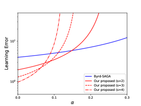
Figure 3: Learning error versus $\alpha$, the fraction of Byzantine workers, for Byrd-SAGA and the proposed method with different $s$. We omit $\delta^{2}$ in the learning errors to compare $C_{\alpha}^{2}$ with $dC_{s\alpha}^{2}$. The number of all workers is $W=30$.

Fig. 3 shows the dependency of learning error on $\alpha:=\frac{B}{W}$ for Byrd-SAGA and the proposed method with different $s$. We omit the outer variation $\delta^{2}$ in the learning errors and compare $C_{\alpha}^{2}$ with $dC_{s\alpha}^{2}$. The number of all workers is set as $W=30$, which is consistent with the setting in the numerical experiments. Observe that when $\alpha$ is small enough, the proposed method has smaller learning error than Byrd-SAGA. This fact depicts the advantage of resampling in reducing the outer variation and handling the non-i.i.d. data. The side-effect of resampling is the tolerance to a smaller fraction of Byzantine workers. Larger $s$ means tolerance to less Byzantine workers. According to the analysis, $s=2$ achieves satisfactory tradeoff between the learning error and the tolerable fraction of Byzantine workers. Therefore, in the numerical experiments we set $s=2$, which is also recommended by [28].

Note that (5) has no closed-form solution, and must be solved with iterative algorithms. Therefore, we often consider $\epsilon$-approximate geometric median, allowing the computed vector and the true geometric median has a gap of $\epsilon$. We use a fast Weiszfeld’s algorithm [35] to compute the $\epsilon$-approximate geometric median in the numerical experiments. For simplicity, in the analysis above we assume $\epsilon=0$. In the appendices, we also consider the case of $\epsilon\neq 0$.

Remark 3. The proof of Theorem 1 is built upon Lemma 1. There is a corresponding [30, Theorem 1] to show the convergence of Byrd-SAGA without resampling. The proof of [30, Theorem 1] is based on [30, Lemma 1], whose difference with our Lemma 1 has been discussed in Section IV-B.

V Numerical Experiments

This section presents numerical experiments to demonstrate the robustness of our proposed method. We consider both convex and nonconvex distributed learning problems. For the convex problem, we focus on the softmax regression on the MNIST [36] dataset. For the nonconvex problem, we train two-layer perceptrons, in which each layer has 50 neurons and the activation function is ‘tanh’, on the MINST and COVTYPE [37] datasets. The attributes of the datasets are described in Table 2. In the i.i.d. case, we use the MNIST dataset, launch 1 central node and $W=30$ workers, and let the data evenly distributed across all workers. In the non-i.i.d. case, we first use the MNIST dataset, launch 1 central node and $W=30$ workers, and let every three workers to evenly share the data from one class. We then use the COVTYPE dataset, launch 1 central node and $W=21$ workers, and also let every three workers to evenly share the data from one class. The numerical experiments are conducted on a server with two Intel(R) Xeon(R) Silver 4216 CPUs and four GeForce RTX 2080 GPUs. The source codes are available at https://github.com/pengj97/Byzantine-robust-variance-reduction

Name	Train	Test	Dimensions	Classes
MNIST	60000	10000	784	10
COVTYPE	11340	565892	54	7

TABLE II: Attributes of the MNIST and COVTYPE datasets.

V-A Benchmark methods

We compare our proposed method with several benchmarks.

Distributed SGD. The distributed SGD aggregates the received messages by returning the mean, and hence has no robustness against Byzantine attacks.

Byrd-SGD. Byrd-SGD aggregates the received messages by returning the geometric median, as shown in (6).

RS-Byrd-SGD. RS-Byrd-SGD first resamples the received messages with $s$-replacement, and then aggregates the results by returning the geometric median.

Krum. Krum aggregates the received messages by returning the one that has the smallest summation of squared distances to its $W-B-2$ nearest neighbors, given by

$$\mathrm{Krum}(\{z_{w},w\in\mathcal{W}\})=z_{w^{*}},$$

$$w^{*}=\arg\min_{w\in\mathcal{W}}\sum_{w\rightarrow w^{\prime}}\|z_{w}-z_{w^{\prime}}\|^{2}.$$

Here $w\rightarrow w^{\prime}$ selects the indexes $w^{\prime}$ of the $W-B-2$ nearest neighbors of $z_{w}$ in $\{z_{w},w\in\mathcal{W}\}$. Note that Krum needs to know the number of Byzantine workers in advance [18].

Byrd-SAGA. Byrd-SAGA aggregates the received messages by returning the geometric median, but the regular workers returns the corrected stochastic gradients, not the stochastic gradients in the above benchmark methods [29, 30].

RSA. RSA is based on model aggregation, not stochastic gradient aggregation in the above benchmark methods. The central node and every worker $w$ maintains iterates $x_{0}^{k}$ and $x_{w}^{k}$, respectively. The update rule of the central node is

$$x_{0}^{k+1}=x_{0}^{k}-\gamma\cdot\lambda\sum_{w\in\mathcal{W}}\mathrm{sign}(x_{0}^{k}-x_{w}^{k}),$$

while the update rule of regular worker $w\in\mathcal{R}$ is

$$x_{w}^{k+1}=x_{w}^{k}-\gamma\cdot\left(f^{\prime}_{w,i_{w}^{k}}(x_{w}^{k})+\lambda\mathrm{sign}(x_{w}^{k}-x_{0}^{k})\right).$$

Here $\mathrm{sign}$ is the element-wise sign function and $\lambda>0$ is the penalty parameter [25].

In the numerical experiments, the batch size is 32. When using resampling, we set $s=2$ by default. All parameters in the benchmark methods are hand-tuned to the best.

V-B Byzantine attacks

We consider the following Byzantine attacks.

Sign-flipping attacks. Every Byzantine worker $w\in\mathcal{B}$ computes its true message $\hat{v}_{w}^{k}$, and then sends $v_{w}^{k}=c\hat{v}_{w}^{k}$ to the central node. Here we set $c=-5$.

Gaussian attacks. Every Byzantine worker $w\in\mathcal{B}$ sends message $v_{w}^{k}$, whose elements follow Gaussian distribution $\mathcal{N}(0,10000)$, to the central node.

Sample-duplicating attacks. The Byzantine workers collude to choose a specific regular worker, and duplicate its message at every time. This amounts to that the Byzantine workers duplicate the data samples of the chosen regular worker. The sample-duplicating attacks are applied in the non-i.i.d. case.

V-C Softmax regression in the i.i.d. case

We carry out numerical experiments in softmax regression on the MNIST dataset. The step size of our proposed method is $\gamma=0.5$. When there exist Byzantine attacks, we uniformly randomly select $B=6$ Byzantine workers.

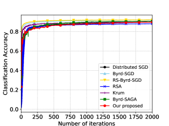
Figure 4: Without Byzantine attacks on i.i.d. MNIST data in softmax regression.

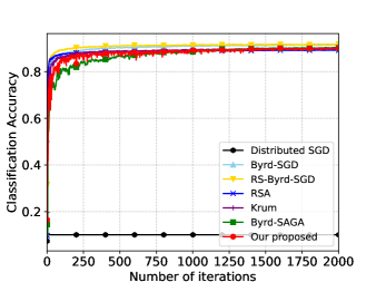
Figure 5: With sign-flipping attacks on i.i.d. MNIST data in softmax regression.

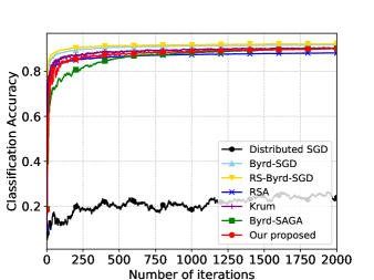
Figure 6: With Gaussian attacks on i.i.d. MNIST data in softmax regression.

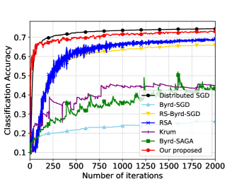
Figure 7: With sample-duplicating attacks on non-i.i.d. MNIST data in softmax regression.

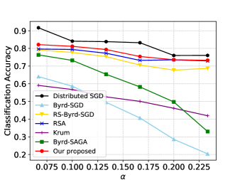
Figure 8: Impact of the fraction of Byzantine workers, with sample-duplicating attacks on non-i.i.d. MNIST data in softmax regression.

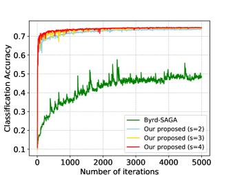
Figure 9: Impact of the resampling size, with sample-duplicating attacks on non-i.i.d. MNIST data in softmax regression.

Without Byzantine attacks. When there exist no Byzantine attacks, all the methods are able to achieve satisfactory classification accuracies, as illustrated in Fig. 4.

Sign-flipping attacks. As depicted in Fig. 5, the distributed SGD is vulnerable and fails under the sign-flipping attacks. The other methods all perform well.

Gaussian attacks. The results of Gaussian attacks are shown in Fig. 6. The distributed SGD also fails, while the other methods have robustness to Gaussian attacks.

V-D Softmax regression in the non-i.i.d. case

Sample-duplicating attacks. We choose $B=6$ workers that originally share the samples of two classes as Byzantine workers. Therefore, these two classes essentially disappear under the sample-duplicating attacks, such that the best possible accuracy is 0.8. For the regular worker that is chosen to be duplicated, its class now has 9 workers out of the total $W=30$. The step size of our proposed method is $\gamma=0.5$. As shown in Fig. 7, our proposed method is able to achieve the classification accuracy of around 0.73. RS-Byrd-SGD also demonstrates robustness since the resampling strategy helps reduce the impact of both inner and outer variations. However, as we have shown in the theoretical analysis, solely using resampling is unable to fully eliminate the inner variation. In contrast, the proposed method introduces SAGA to address this issue, yielding enhanced classification accuracy. RSA works well since it is developed to handle the non-i.i.d. case. The other Byzantine-robust methods, Byrd-SGD, Krum and Byrd-SAGA, all show degraded performance since they are essentially designed for distributed i.i.d. data.

Impact of the fraction of Byzantine workers $\alpha$. Theorem 1 and Fig. 3 demonstrate that the learning error of the proposed method is monotonically increasing when the fraction of Byzantine workers $\alpha$ increases. This theoretical result is validated by Fig. 8. The other experimental settings are the same as those in Fig. 7. The classification accuracies of all the methods degrade when $\alpha$ increases. Compared to other benchmark methods, our proposed method is comparatively insensitive to the variation of $\alpha$.

Impact of the resampling size $s$. Theorem 1 and Fig. 3 also shows that the learning error of the proposed method is dependent on the resampling size $s$. Fig. 9 depicts how the classification accuracies vary with respect to different $s$. The other experimental settings are the same as those in Fig. 7. When $s=1$, our proposed method degenerates to Byrd-SAGA, which is not Byzantine-robust in the non-i.i.d. case. When $s=3$ and $s=4$, for these particular attacks, the proposed method still performs well, although the fraction of Byzantine workers $\alpha=\frac{1}{5}$ exceeds the theoretically tolerable bound $\frac{1}{2s}$.

V-E Neural network training in the non-i.i.d. case

Sample-duplicating attacks on MNIST. We choose $B=3$ workers that originally share the samples of one class as Byzantine workers, such that the best possible accuracy is 0.9 under the sample-duplicating attacks. The step size of our proposed method is $\gamma=0.1$. We compare Byrd-SGD, RS-Byrd-SGD, Byrd-SAGA and our proposed method in Fig. 10. Byrd-SGD fails, but Byrd-SAGA is able to attain favorable classification accuracy since the ratio of Byzantine workers is only $10\%$. Among the two methods developed for the non-i.i.d. case, our proposed method outperforms RS-Byrd-SGD. The performance gain of Byrd-SAGA over Byrd-SGD and that of the proposed method over RS-Byrd-SGD are both due to the elimination of inner variation.

Sample-duplicating attacks on COVTYPE. We choose $B=3$ workers that originally share the samples of one class as Byzantine workers, such that the best possible accuracy is 0.86 under the sample-duplicating attacks. The step size of our proposed method is $\gamma=0.1$. As shown in Fig. 11, Byrd-SGD is still the worst. However, Byrd-SAGA and RS-Byrd-SGD are both remarkably outperformed by our proposed method, since the ratio of Byzantine workers is now raised to $14\%$. Therefore, eliminating the inner variation and reducing the outer variation are of particular importance as a larger portion of received messages are Byzantine.

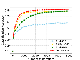
Figure 10: Classification accuracy with sample-duplicating attacks on non-i.i.d. MNIST data in neural network training.

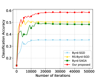
Figure 11: Classification accuracy with sample-duplicating attacks on non-i.i.d. COVTYPE data in neural network training.

VI Conclusions

We develop a Byzantine-robust variance-reduced method to deal with the federated learning problem with distributed non-i.i.d. data. To reduce the impact of stochastic gradient noise that hinders the resistance to Byzantine attacks, we adopt the resampling strategy and SAGA to reduce the outer variation and fully eliminate the inner variation. The variance-reduced messages are then aggregated by geometric median. Theoretical results show that the proposed method can reach a neighborhood of the optimal solution with linear convergence rate and the learning error is determined by the number of Byzantine workers. Numerical experiments demonstrate the robustness of our proposed method. In the future work, we will investigate the elimination of outer variation, and the combination of variance-reduced methods with other robust aggregation rules.

Appendix A Proof of Lemma 1

We begin with reviewing the supporting lemma.

Lemma 3.

[28, Proposition 1] Let $\{z_{w},w\in\mathcal{W}\}$ be a set of vectors, and generate from it a new set $\{\tilde{z}_{w},w\in\mathcal{W}\}$ using the resampling strategy with $s$-replacement. When $B<\frac{W}{s}$, there exists a set $\mathcal{R}^{\prime}\subseteq\mathcal{W}$ with at least $W-sB$ elements, such that for any $w^{\prime}\in\mathcal{R}^{\prime}$ it holds that

$$\mathbb{E}\tilde{z}_{w^{\prime}}=\frac{1}{R}\sum_{w\in\mathcal{R}}z_{w},$$ (23)

$$\mathbb{E}\|\tilde{z}_{w^{\prime}}-\mathbb{E}\tilde{z}_{w^{\prime}}\|^{2}=\frac{d}{R}\sum_{w\in\mathcal{R}}\left\|z_{w}-\frac{1}{R}\sum_{u\in\mathcal{R}}z_{u}\right\|^{2},$$ (24)

where $d:=\frac{W-1}{sW-1}$ and the expectation $\mathbb{E}$ is taken over the resampling process.

Lemma 3 shows that after resampling, the expectations of at least $W-sB$ elements are the average of $\{z_{w},w\in\mathcal{R}\}$. Their variance $\mathbb{E}\|\tilde{z}_{w^{\prime}}-\mathbb{E}\tilde{z}_{w^{\prime}}\|^{2}$ reduces by a factor of $\frac{1}{d}$ relative to the variation $\frac{1}{R}\sum_{w\in\mathcal{R}}\|z_{w}-\frac{1}{R}\sum_{w\in\mathcal{R}}z_{w}\|^{2}$. Note that $\frac{1}{d}$ is close to $s$ if $W$ is sufficiently large. The properties of these $W-sB$ elements are further investigated in Lemma 2, whose proof is as follows.

Proof.

We decompose $\frac{1}{|\mathcal{R^{\prime}}|}\sum_{w^{\prime}\in\mathcal{R}^{\prime}}\mathbb{E}\|\tilde{z}_{w^{\prime}}-\bar{z}\|^{2}$ into two terms

$$\frac{1}{|\mathcal{R^{\prime}}|}\sum_{w^{\prime}\in\mathcal{R}^{\prime}}\mathbb{E}\|\tilde{z}_{w^{\prime}}-\bar{z}\|^{2}$$ (25)

$$= \frac{1}{|\mathcal{R^{\prime}}|}\sum_{w^{\prime}\in\mathcal{R}^{\prime}}\mathbb{E}\left\|\tilde{z}_{w^{\prime}}-\frac{1}{R}\sum_{w\in\mathcal{R}}z_{w}\right\|^{2}+\mathbb{E}\left\|\frac{1}{R}\sum_{w\in\mathcal{R}}z_{w}-\bar{z}\right\|^{2}$$

$$= \frac{d}{R}\sum_{w\in\mathcal{R}}\mathbb{E}\left\|z_{w}-\frac{1}{R}\sum_{u\in\mathcal{R}}z_{u}\right\|^{2}+\mathbb{E}\left\|\frac{1}{R}\sum_{w\in\mathcal{R}}z_{w}-\bar{z}\right\|^{2},$$

where the last equality comes from Lemma 3 that for any $w^{\prime}\in\mathcal{R}^{\prime}$ it holds

$$\mathbb{E}\left\|\tilde{z}_{w^{\prime}}-\frac{1}{R}\sum_{w\in\mathcal{R}}z_{w}\right\|^{2}= \mathbb{E}\left\|\tilde{z}_{w^{\prime}}-\mathbb{E}\tilde{z}_{w^{\prime}}\right\|^{2}$$

$$= \frac{d}{R}\sum_{w\in\mathcal{R}}\mathbb{E}\left\|z_{w}-\frac{1}{R}\sum_{u\in\mathcal{R}}z_{u}\right\|^{2}.$$

The first term at the right-hand side of (25) can be further decomposed into three terms

$$\frac{1}{R}\sum_{w\in\mathcal{R}}\mathbb{E}\left\|z_{w}-\frac{1}{R}\sum_{u\in\mathcal{R}}z_{u}\right\|^{2}$$ (26)

$$= \frac{1}{R}\sum_{w\in\mathcal{R}}\mathbb{E}\Bigg{\|}(z_{w}-\mathbb{E}z_{w})+\left(\mathbb{E}z_{w}-\frac{1}{R}\sum_{u\in\mathcal{R}}\mathbb{E}z_{u}\right)$$

$$+\left(\frac{1}{R}\sum_{u\in\mathcal{R}}\mathbb{E}z_{u}-\frac{1}{R}\sum_{u\in\mathcal{R}}z_{u}\right)\Bigg{\|}^{2}$$

$$= \frac{1}{R}\sum_{w\in\mathcal{R}}\mathbb{E}\left\|z_{w}-\mathbb{E}z_{w}\right\|^{2}+\frac{1}{R}\sum_{w\in\mathcal{R}}\left\|\mathbb{E}z_{w}-\frac{1}{R}\sum_{u\in\mathcal{R}}\mathbb{E}z_{u}\right\|^{2}$$

$$+ \mathbb{E}\left\|\frac{1}{R}\sum_{w\in\mathcal{R}}z_{w}-\frac{1}{R}\sum_{w\in\mathcal{R}}\mathbb{E}z_{w}\right\|^{2}$$

$$+ \underbrace{\frac{2}{R}\sum_{w\in\mathcal{R}}\mathbb{E}\left\langle z_{w}-\mathbb{E}z_{w},\mathbb{E}z_{w}-\frac{1}{R}\sum_{u\in\mathcal{R}}\mathbb{E}z_{u}\right\rangle}_{T_{1}}$$

$$+ \underbrace{\frac{2}{R}\sum_{w\in\mathcal{R}}\mathbb{E}\left\langle\mathbb{E}z_{w}-\frac{1}{R}\sum_{u\in\mathcal{R}}\mathbb{E}z_{u},\frac{1}{R}\sum_{u\in\mathcal{R}}\mathbb{E}z_{u}-\frac{1}{R}\sum_{u\in\mathcal{R}}z_{u}\right\rangle}_{T_{2}}$$

$$+ \underbrace{\frac{2}{R}\sum_{w\in\mathcal{R}}\mathbb{E}\left\langle z_{w}-\mathbb{E}z_{w},\frac{1}{R}\sum_{u\in\mathcal{R}}\mathbb{E}z_{u}-\frac{1}{R}\sum_{u\in\mathcal{R}}z_{u}\right\rangle}_{T_{3}}$$

$$= \frac{1}{R}\sum_{w\in\mathcal{R}}\mathbb{E}\left\|z_{w}-\mathbb{E}z_{w}\right\|^{2}+\frac{1}{R}\sum_{w\in\mathcal{R}}\left\|\mathbb{E}z_{w}-\frac{1}{R}\sum_{u\in\mathcal{R}}\mathbb{E}z_{u}\right\|^{2}$$

$$-\mathbb{E}\left\|\frac{1}{R}\sum_{w\in\mathcal{R}}z_{w}-\frac{1}{R}\sum_{w\in\mathcal{R}}\mathbb{E}z_{w}\right\|^{2}.$$

To see how to reach the last equality, we check the three cross terms. The first cross term can be cancelled by

$$T_{1}= \frac{2}{R}\sum_{w\in\mathcal{R}}\mathbb{E}\left\langle z_{w}-\mathbb{E}z_{w},\mathbb{E}z_{w}-\frac{1}{R}\sum_{u\in\mathcal{R}}\mathbb{E}z_{u}\right\rangle$$ (27)

$$= \frac{2}{R}\sum_{w\in\mathcal{R}}\left\langle\underbrace{\mathbb{E}z_{w}-\mathbb{E}z_{w}}_{=0},\mathbb{E}z_{w}-\frac{1}{R}\sum_{u\in\mathcal{R}}\mathbb{E}z_{u}\right\rangle$$

$$= 0.$$

Similarly, the second cross term can be cancelled by

$$T_{2}= \frac{2}{R}\sum_{w\in\mathcal{R}}\mathbb{E}\left\langle\mathbb{E}z_{w}-\frac{1}{R}\sum_{u\in\mathcal{R}}\mathbb{E}z_{u},\frac{1}{R}\sum_{u\in\mathcal{R}}\mathbb{E}z_{u}-\frac{1}{R}\sum_{u\in\mathcal{R}}z_{u}\right\rangle$$ (28)

$$= \frac{2}{R}\sum_{w\in\mathcal{R}}\left\langle\mathbb{E}z_{w}-\frac{1}{R}\sum_{u\in\mathcal{R}}\mathbb{E}z_{u},\underbrace{\frac{1}{R}\sum_{u\in\mathcal{R}}\mathbb{E}z_{u}-\frac{1}{R}\sum_{u\in\mathcal{R}}\mathbb{E}z_{u}}_{=0}\right\rangle$$

$$= 0.$$

The third cross term equals to

$$T_{3}= \frac{2}{R}\sum_{w\in\mathcal{R}}\mathbb{E}\left\langle z_{w}-\mathbb{E}z_{w},\frac{1}{R}\sum_{u\in\mathcal{R}}\mathbb{E}z_{u}-\frac{1}{R}\sum_{u\in\mathcal{R}}z_{u}\right\rangle$$ (29)

$$= 2\mathbb{E}\left\langle\frac{1}{R}\sum_{w\in\mathcal{R}}z_{w}-\frac{1}{R}\sum_{w\in\mathcal{R}}\mathbb{E}z_{w},\frac{1}{R}\sum_{u\in\mathcal{R}}\mathbb{E}z_{u}-\frac{1}{R}\sum_{u\in\mathcal{R}}z_{u}\right\rangle$$

$$= -2\mathbb{E}\left\|\frac{1}{R}\sum_{w\in\mathcal{R}}z_{w}-\frac{1}{R}\sum_{w\in\mathcal{R}}\mathbb{E}z_{w}\right\|^{2}.$$

Substituting (26) into (25) and using the definition $\bar{z}:=\frac{1}{R}\sum_{w\in\mathcal{R}}\mathbb{E}z_{w}$, we have

$$\frac{1}{|\mathcal{R^{\prime}}|}\sum_{w^{\prime}\in\mathcal{R}^{\prime}}\mathbb{E}\|\tilde{z}_{w^{\prime}}-\bar{z}\|^{2}$$ (30)

$$= \frac{d}{R}\sum_{w\in\mathcal{R}}\mathbb{E}\left\|z_{w}-\mathbb{E}z_{w}\right\|^{2}+\frac{d}{R}\sum_{w\in\mathcal{R}}\left\|\mathbb{E}z_{w}-\frac{1}{R}\sum_{u\in\mathcal{R}}\mathbb{E}z_{u}\right\|^{2}$$

$$+(1-d)\mathbb{E}\left\|\frac{1}{R}\sum_{w\in\mathcal{R}}z_{w}-\frac{1}{R}\sum_{w\in\mathcal{R}}\mathbb{E}z_{w}\right\|^{2}$$

$$= \frac{d}{R}\sum_{w\in\mathcal{R}}\mathbb{E}\left\|z_{w}-\mathbb{E}z_{w}\right\|^{2}+\frac{d}{R}\sum_{w\in\mathcal{R}}\left\|\mathbb{E}z_{w}-\bar{z}\right\|^{2}$$

$$+\frac{1-d}{R^{2}}\sum_{w\in\mathcal{R}}\mathbb{E}\left\|z_{w}-\mathbb{E}z_{w}\right\|^{2}$$

$$= \left(d+\frac{1-d}{R}\right)\frac{1}{R}\sum_{w\in\mathcal{R}}\mathbb{E}\left\|z_{w}-\mathbb{E}z_{w}\right\|^{2}$$

$$+\frac{d}{R}\sum_{w\in\mathcal{R}}\left\|\mathbb{E}z_{w}-\bar{z}\right\|^{2}.$$

The second equality in (30) comes from

$$\mathbb{E}\left\|\frac{1}{R}\sum_{w\in\mathcal{R}}z_{w}-\frac{1}{R}\sum_{w\in\mathcal{R}}\mathbb{E}z_{w}\right\|^{2}$$ (31)

$$= \mathbb{E}\left\|\frac{1}{R}\sum_{w\in\mathcal{R}}(z_{w}-\mathbb{E}z_{w})\right\|^{2}$$

$$= \frac{1}{R^{2}}\sum_{w\in\mathcal{R}}\mathbb{E}\left\|z_{w}-\mathbb{E}z_{w}\right\|^{2}$$

$$+\sum_{w,u\in\mathcal{R}\atop w\neq u}\mathbb{E}\left\langle\frac{1}{R}(z_{w}-\mathbb{E}z_{w}),\frac{1}{R}(z_{u}-\mathbb{E}z_{u})\right\rangle$$

$$= \frac{1}{R^{2}}\sum_{w\in\mathcal{R}}\mathbb{E}\left\|z_{w}-\mathbb{E}z_{w}\right\|^{2},$$

where the last equality is due to the fact that the random vectors in $\{z_{w},w\in\mathcal{R}\}$ are independent. This completes the proof. ∎

With Lemma 2, the proof of Lemma 1 is straightforward.

Lemma 4.

(Full version of Lemma 1) Let $\{z_{w},w\in\mathcal{W}\}$ be a subset of random vectors distributed in a normed vector space and the random vectors in $\{z_{w},w\in\mathcal{R}\}$ are independent. Generate from $\{z_{w},w\in\mathcal{W}\}$ a new set $\{\tilde{z}_{w},w\in\mathcal{W}\}$ using the resampling strategy with $s$-replacement. It holds when $B<\frac{W}{2s}$ that

$$\mathbb{E}\|\mathrm{geomed}\left(\{\tilde{z}_{w},w\in\mathcal{W}\}\right)-\bar{z}\|^{2}\$$ (32)

$$\leq \left(d+\frac{1-d}{R}\right)\frac{C_{s\alpha}^{2}}{R}\sum_{w\in\mathcal{R}}{\mathbb{E}\|z_{w}-\mathbb{E}z_{w}\|^{2}}$$

$$+\frac{dC_{s\alpha}^{2}}{R}\sum_{w\in\mathcal{R}}{\|\mathbb{E}z_{w}-\bar{z}\|^{2}},$$

where $\bar{z}:=\frac{1}{R}\sum_{w\in\mathcal{R}}\mathbb{E}z_{w}$, $\alpha:=\frac{B}{W}$, $C_{s\alpha}:=\frac{2-2s\alpha}{1-2s\alpha}$, $d:=\frac{W-1}{sW-1}$, and $\mathbb{E}$ is taken over the random vectors and the resampling process. Define $\tilde{z}_{\epsilon}^{*}$ as an $\epsilon$-approximate geometric median of $\{\tilde{z}_{w},w\in\mathcal{W}\}$. It holds when $B<\frac{W}{2s}$ that

$$\mathbb{E}\|\tilde{z}_{\epsilon}^{*}-\bar{z}\|^{2}$$ (33)

$$\leq \left(d+\frac{1-d}{R}\right)\frac{2C_{s\alpha}^{2}}{R}\sum_{w\in\mathcal{R}}{\mathbb{E}\|z_{w}-\mathbb{E}z_{w}\|^{2}}$$

$$+\frac{2dC_{s\alpha}^{2}}{R}\sum_{w\in\mathcal{R}}{\|\mathbb{E}z_{w}-\bar{z}\|^{2}}+\frac{2\epsilon^{2}}{(W-2sB)^{2}}.$$

Proof.

We firstly prove (32). As Lemma 3 claims, when $B<\frac{W}{s}$, there exists a set $\mathcal{R}^{\prime}\subseteq\mathcal{W}$ with at least $W-sB$ elements, such that for any $w^{\prime}\in\mathcal{R}^{\prime}$, (23) and (24) hold true. When $B<\frac{W}{2s}$, $\frac{|\mathcal{R}^{\prime}|}{W}>\frac{1}{2}$. With [30, Lemma 2], it holds that

$$\mathbb{E}\|\mathop{\text{geomed}}(\{\tilde{z}_{w},w\in\mathcal{W}\})-\bar{z}\|^{2}$$ (34)

$$= \mathbb{E}\|\mathop{\text{geomed}}(\{\tilde{z}_{w}-\bar{z},w\in\mathcal{W}\})\|^{2}$$

$$\leq \frac{C_{s\alpha}^{2}}{|\mathcal{R^{\prime}}|}\sum_{w^{\prime}\in\mathcal{R}^{\prime}}\mathbb{E}\|\tilde{z}_{w^{\prime}}-\bar{z}\|^{2}.$$

Applying Lemma 2 completes the proof of (32).

Next, we prove (33). With [30, Lemma 3], it holds that

$$\mathbb{E}\|\tilde{z}_{\epsilon}^{*}-\bar{z}\|^{2}$$ (35)

$$\leq \frac{2C_{s\alpha}^{2}}{|\mathcal{R^{\prime}}|}\sum_{w^{\prime}\in\mathcal{R}^{\prime}}\mathbb{E}\|\tilde{z}_{w^{\prime}}-\bar{z}\|+\frac{2\epsilon^{2}}{(W-2|\mathcal{R^{\prime}}|)^{2}}$$

$$\leq \frac{2C_{s\alpha}^{2}}{|\mathcal{R^{\prime}}|}\sum_{w^{\prime}\in\mathcal{R}^{\prime}}\mathbb{E}\|\tilde{z}_{w^{\prime}}-\bar{z}\|+\frac{2\epsilon^{2}}{(W-2sB)^{2}}.$$

Applying Lemma 2 completes the proof of (33). ∎

Appendix B Proof of Theorem 1

To prove Theorem 1, we review the following supporting lemma for SAGA.

Lemma 5.

[30, Lemmas 4 and 5] Under Assumption 1, if all regular workers $w\in\mathcal{W}$ update $\phi_{w,i_{w}^{k}}^{k}$ and $v_{w}^{k}$ according to (9) and (10), then the corrected stochastic gradient $v_{w}^{k}$ satisfies

$$\mathbb{E}\|v_{w}^{k}-f_{w}^{\prime}(x^{k})\|^{2}\leq L^{2}\frac{1}{J}\sum_{j=1}^{J}\|x^{k}-\phi_{w,j}^{k}\|^{2},\quad\forall w\in\mathcal{W},$$ (36)

and

$$\frac{1}{R}\sum_{w\in\mathcal{R}}\mathbb{E}\|v_{w}^{k}-f_{w}^{\prime}(x^{k})\|^{2}\leq L^{2}S^{k},$$ (37)

where $S^{k}$ is defined as

$$S^{k}:=\frac{1}{R}\sum_{w\in\mathcal{R}}\frac{1}{J}\sum_{j=1}^{J}\|x^{k}-\phi_{w,j}^{k}\|^{2}.$$ (38)

Further, $S^{k}$ satisfies

$$\mathbb{E}S^{k+1}\leq 4J\mathbb{E}\|x^{k+1}-x^{k}+\gamma f^{\prime}(x^{k})\|^{2}$$ (39)

$$+4J\gamma^{2}L^{2}\|x^{k}-x^{*}\|^{2}+(1-\frac{1}{J^{2}})S^{k}.$$

Theorem 2.

(Full version of Theorem 1) Under Assumptions 1 and 2, if the number of Byzantine workers satisfies $B<\frac{W}{2s}$ and the step size satisfies

$$\gamma\leq\frac{\mu}{2\sqrt{10}J^{2}L^{2}C_{s\alpha}},$$

then the iterate $x^{k}$ generated by the proposed method in Algorithm 2 satisfies

$$\mathbb{E}\|x^{k}-x^{*}\|^{2}\leq(1-\frac{\gamma\mu}{2})^{k}\Delta_{1}+\Delta_{2},$$ (40)

where

$$\Delta_{1}:=\|x^{0}-x^{*}\|^{2}-\Delta_{2},$$ (41)

$$\Delta_{2}:=\frac{5dC_{s\alpha}^{2}\delta^{2}}{\mu^{2}},$$ (42)

while $\alpha:=\frac{B}{W}$, $C_{s\alpha}:=\frac{2-2s\alpha}{1-2s\alpha}$, $d:=\frac{W-1}{sW-1}$, and $\mathbb{E}$ denote the expectation with respect to all random variables $i_{w}^{k}$ and the resampling processes. On the other hand, when the step size satisfies

$$\gamma\leq\frac{\mu}{4\sqrt{5}J^{2}L^{2}C_{s\alpha}},$$

the iterate $x^{k}$ generated by the proposed method in Algorithm 2 with $\epsilon$-approximate geometric median aggregation satisfies

$$\mathbb{E}\|x^{k}-x^{*}\|^{2}\leq(1-\frac{\gamma\mu}{2})^{k}\Delta_{1}+2\Delta_{2}+\frac{10\epsilon^{2}}{\mu^{2}(W-2sB)^{2}}.$$ (43)

Proof.

For simplicity, we only prove (40). According to the proof of Theorem 1 in [30], when

$$\gamma\leq\frac{\mu}{2L^{2}},$$ (44)

it holds that

$$\mathbb{E}\|x^{k+1}-x^{*}\|^{2}$$ (45)

$$\leq (1-\gamma\mu)\|x^{k}-x^{*}\|^{2}+\frac{2}{\gamma\mu}\mathbb{E}\|x^{k+1}-x^{k}+\gamma f^{\prime}(x^{k})\|^{2}.$$

Then, we construct a Lyapunov function $T_{1}^{k}$ as

$$T_{1}^{k}:=\|x^{k}-x^{*}\|^{2}+c_{1}S^{k},$$ (46)

where $c_{1}$ is any positive constant. Since $S^{k}$ is non-negative according to the definition in (38), we know that $T_{1}^{k}$ is also non-negative. Substituting (39) and (45) into (46) yields

$$\mathbb{E}T_{1}^{k+1}$$ (47)

$$\leq (1-\gamma\mu+4c_{1}J\gamma^{2}L^{2})\|x^{k}-x^{*}\|^{2}$$

$$+ (\frac{2}{\gamma\mu}+4c_{1}J)\mathbb{E}\|x^{k+1}-x^{k}+\gamma f^{\prime}(x^{k})\|^{2}$$

$$+ (1-\frac{1}{J^{2}})c_{1}S^{k}.$$

Note that the second term at the right-hand side of (47) can be bounded with the help of Lemma 4, as

$$\mathbb{E}\|x^{k+1}-x^{k}+\gamma f^{\prime}(x^{k})\|^{2}$$ (48)

$$= \gamma^{2}\mathbb{E}\|\mathrm{geomed}\left(\{\tilde{v}_{w}^{k},w\in\mathcal{W}\}\right)-f^{\prime}(x^{k})\|^{2}$$

$$\leq \gamma^{2}\left(d+\frac{1-d}{R}\right)\frac{C_{s\alpha}^{2}}{R}\sum_{w\in\mathcal{R}}{\mathbb{E}\|v_{w}^{k}-f_{w}^{\prime}(x^{k})\|^{2}}$$

$$+\gamma^{2}\frac{dC_{s\alpha}^{2}}{R}\sum_{w\in\mathcal{R}}{\|f_{w}^{\prime}(x^{k})-f^{\prime}(x^{k})\|^{2}}$$

$$\leq \gamma^{2}\left(d+\frac{1-d}{R}\right)C_{s\alpha}^{2}L^{2}S^{k}+\gamma^{2}dC_{s\alpha}^{2}\delta^{2},$$

where the last inequality comes from Lemma 5 and Assumption 2. Therefore, we have

$$\mathbb{E}T_{1}^{k+1}$$ (49)

$$\leq (1-\gamma\mu+4c_{1}J\gamma^{2}L^{2})\|x^{k}-x^{*}\|^{2}$$

$$+ \bigg{(}1-\frac{1}{J^{2}}\bigg{)}c_{1}S^{k}$$

$$+ \bigg{(}\frac{2}{\gamma\mu}+4c_{1}J\bigg{)}\bigg{(}d+\frac{1-d}{R}\bigg{)}C_{s\alpha}^{2}\gamma^{2}L^{2}S^{k}.$$

$$+ \gamma^{2}\bigg{(}\frac{2}{\gamma\mu}+4c_{1}J\bigg{)}dC_{s\alpha}^{2}\delta^{2}$$

If we constrain the step size $\gamma$ as

$$4c_{1}J\gamma^{2}L^{2}\leq\frac{\gamma\mu}{2},$$ (50)

then the coefficients in (49) satisfy

$$1-\gamma\mu+4c_{1}J\gamma^{2}L^{2} \leq 1-\frac{\gamma\mu}{2},$$ (51)

$$\frac{2}{\gamma\mu}+4c_{1}J \leq\frac{2}{\gamma\mu}+\frac{\mu}{2\gamma L^{2}}\leq\frac{5}{2\gamma\mu}.$$ (52)

Therefore, we can bound $\mathbb{E}T^{k+1}$ by

$$\mathbb{E}T_{1}^{k+1} \leq(1-\frac{\gamma\mu}{2})\|x^{k}-x^{*}\|^{2}+\frac{5\gamma}{2\mu}dC_{s\alpha}^{2}\delta^{2}$$ (53)

$$+\bigg{(}\bigg{(}1-\frac{1}{J^{2}}\bigg{)}c_{1}+\frac{5\gamma}{2\mu}\bigg{(}d+\frac{1-d}{R}\bigg{)}C_{s\alpha}^{2}L^{2}\bigg{)}S^{k}.$$

Similarly, if $\gamma$ and $c_{1}$ are chosen such that

$$\frac{\gamma\mu}{2}<\frac{1}{2J^{2}},$$ (54)

and

$$c_{1}= \frac{5J^{2}\gamma L^{2}(d+(1-d)/R)C_{s\alpha}^{2}}{\mu}$$ (55)

$$\geq \frac{5\gamma L^{2}(d+(1-d)/R)C_{s\alpha}^{2}/2}{\mu(1/J^{2}-\gamma\mu/2)},$$

then the coefficient in (53) satisfies

$$\bigg{(}1-\frac{1}{J^{2}}\bigg{)}c_{1}+\frac{5\gamma}{2\mu}\bigg{(}d+\frac{1-d}{R}\bigg{)}C_{s\alpha}^{2}L^{2}\leq(1-\frac{\gamma\mu}{2})c_{1}.$$ (56)

Hence, (53) becomes

$$\mathbb{E}T_{1}^{k+1}$$ (57)

$$\leq (1-\frac{\gamma\mu}{2})\|x^{k}-x^{*}\|^{2}+(1-\frac{\gamma\mu}{2})c_{1}S^{k}+\frac{5\gamma}{2\mu}dC_{s\alpha}^{2}\delta^{2}$$

$$= (1-\frac{\gamma\mu}{2})T_{1}^{k}+\frac{5\gamma}{2\mu}dC_{s\alpha}^{2}\delta^{2}.$$

Using telescopic cancellation on (57) from time 1 to time $k$, we have

$$\mathbb{E}T_{1}^{k}\leq(1-\frac{\gamma\mu}{2})^{k}\bigg{[}T_{1}^{0}-\Delta_{2}\bigg{]}+\Delta_{2}.$$ (58)

Here and thereafter, the expectation is taken over $i_{w}^{k}$ for all regular workers $w\in\mathcal{R}$. The definition of the Lyapunov function in (46) implies that

$$\mathbb{E}\|x^{k}-x^{*}\|^{2}\leq\mathbb{E}T_{1}^{k}\leq(1-\frac{\gamma\mu}{2})^{k}\Delta_{1}+\Delta_{2}.$$ (59)

In our derivation so far, the constraint on the step size $\gamma$ (c.f. (44), (50) and (54)) is

$$\gamma\leq\min \bigg{\{}\frac{\mu}{2L^{2}},\frac{1}{J^{2}\mu},$$ (60)

$$\frac{\mu}{2\sqrt{10}J^{3/2}L^{2}C_{s\alpha}(d+(1-d)/R)^{1/2}}\bigg{\}}.$$

Therefore, we simply choose

$$\gamma\leq\frac{\mu}{2\sqrt{10}J^{2}L^{2}C_{s\alpha}},$$ (61)

which completes the proof. ∎

Appendix C Convergence Property of RS-Byrd-SGD

Now we show that the learning error of RS-Byrd-SGD, whose update is given by

$$x^{k+1}=x^{k}-\gamma\cdot\mathrm{geomed}\left(\{\tilde{g}_{w}^{k},w\in\mathcal{W}\}\right),$$ (62)

is in the order of ${\cal O}((d+\frac{1-d}{R})C_{s\alpha}^{2}\sigma^{2}+dC_{s\alpha}^{2}\delta^{2})$.

Theorem 3.

Under Assumptions 1, 2 and 3, if the number of Byzantine workers satisfies $B<\frac{W}{2s}$ and the step size satisfies

$$\gamma\leq\frac{\mu}{2L^{2}},$$

then the iterate $x^{k}$ generated by RS-Byrd-SGD satisfies

$$\mathbb{E}\|x^{k}-x^{*}\|^{2}\leq(1-\gamma\mu)^{k}\Delta_{1}+\Delta_{2},$$ (63)

where

$$\Delta_{1}:=\|x^{0}-x^{*}\|^{2}-\Delta_{2},$$ (64)

$$\Delta_{2}:=\frac{2}{\mu^{2}}\bigg{(}\bigg{(}d+\frac{1-d}{R}\bigg{)}C_{s\alpha}^{2}\sigma^{2}+dC_{s\alpha}^{2}\delta^{2}\bigg{)}.$$ (65)

while $\alpha:=\frac{B}{W}$, $C_{s\alpha}:=\frac{2-2s\alpha}{1-2s\alpha}$, $d:=\frac{W-1}{sW-1}$, and $\mathbb{E}$ denote the expectation with respect to all random variables $i_{w}^{k}$ and the resampling processes. On the other hand, the iterate $x^{k}$ generated by RS-Byrd-SGD with $\epsilon$-approximate geometric median aggregation satisfies

$$\mathbb{E}\|x^{k}-x^{*}\|^{2}\leq(1-\gamma\mu)^{k}\Delta_{1}+2\Delta_{2}+\frac{4\epsilon^{2}}{\mu^{2}(W-2sB)^{2}}.$$ (66)

Proof.

For simplicity, we only prove (63). Note that inequality (45) is still true for RS-Byrd-SGD with $\gamma<\frac{\mu}{2L^{2}}$. The only difference is that we need to bound the term $\mathbb{E}\|x^{k+1}-x^{k}+\gamma f^{\prime}(x^{k})\|$ with Lemma 4, as

$$\mathbb{E}\|x^{k+1}-x^{k}+\gamma f^{\prime}(x^{k})\|$$ (67)

$$= \gamma^{2}\mathbb{E}\|\mathrm{geomed}\left(\{\tilde{g}_{w}^{k},w\in\mathcal{W}\}\right)-f^{\prime}(x^{k})\|^{2}$$

$$\leq \gamma^{2}\bigg{(}\bigg{(}d+\frac{1-d}{R}\bigg{)}\frac{C_{s\alpha}^{2}}{R}\sum_{w\in\mathcal{R}}\mathbb{E}\|f^{\prime}_{w,i_{w}^{k}}(x^{k})-f^{\prime}_{w}(x^{k})\|^{2}$$

$$+\frac{dC_{s\alpha}^{2}}{R}\sum_{w\in\mathcal{R}}\|f^{\prime}_{w}(x^{k})-f^{\prime}(x^{k})\|^{2}\bigg{)}$$

$$\leq \gamma^{2}\bigg{(}\bigg{(}d+\frac{1-d}{R}\bigg{)}C_{s\alpha}^{2}\sigma^{2}+dC_{s\alpha}^{2}\delta^{2}\bigg{)}.$$

Therefore, we have

$$\mathbb{E}\|x^{k+1}-x^{*}\|^{2}$$ (68)

$$\leq (1-\gamma\mu)\|x^{k}-x^{*}\|^{2}+\frac{2}{\gamma\mu}\mathbb{E}\|x^{k+1}-x^{k}+\gamma f^{\prime}(x^{k})\|^{2}$$

$$\leq (1-\gamma\mu)\|x^{k}-x^{*}\|^{2}$$

$$+\frac{2\gamma}{\mu}\bigg{(}\bigg{(}d+\frac{1-d}{R}\bigg{)}C_{s\alpha}^{2}\sigma^{2}+dC_{s\alpha}^{2}\delta^{2}\bigg{)}.$$

Here and thereafter, the expectation is taken over $i_{w}^{k}$ for all regular workers $w\in\mathcal{R}$. Using telescopic cancellation on (68) completes the proof. ∎

References

- [1] J. Konečnỳ, H. B. McMahan, D. Ramage, and P. Richtárik, “Federated optimization: Distributed machine learning for on-device intelligence,” arXiv preprint arXiv:1610.02527, 2016.
- [2] H. B. McMahan, E. Moore, D. Ramage, and B. A. y Arcas, “Federated learning of deep networks using model averaging.” arXiv preprint arXiv:1602.05629, 2016.
- [3] Q. Yang, Y. Liu, T. Chen, and Y. Tong, “Federated machine learning: Concept and applications,” ACM Transactions on Intelligent Systems and Technology, vol. 10, no. 2, pp. 1–19, 2019.
- [4] P. Kairouz, H. B. McMahan, B. Avent, A. Bellet, M. Bennis, A. N. Bhagoji, K. Bonawitz, Z. Charles, G. Cormode, R. Cummings et al., “Advances and open problems in federated learning,” arXiv preprint arXiv:1912.04977, 2019.
- [5] J. Park, S. Samarakoon, M. Bennis, and M. Debbah, “Wireless network intelligence at the edge,” Proceedings of the IEEE, vol. 107, no. 11, pp. 2204–2239, 2019.
- [6] T. Zeng, O. Semiari, M. Mozaffari, M. Chen, W. Saad, and M. Bennis, “Federated learning in the sky: Joint power allocation and scheduling with uav swarms,” in IEEE International Conference on Communications, 2020, pp. 1–6.
- [7] L. Lamport, R. E. Shostak, and M. C. Pease, “The byzantine generals problem,” ACM Transactions on Programming Languages and Systems, vol. 4, no. 3, pp. 382–401, 1982.
- [8] Y. Chen, L. Su, and J. Xu, “Distributed statistical machine learning in adversarial settings: Byzantine gradient descent,” ACM on Measurement and Analysis of Computing Systems, vol. 1, no. 2, pp. 1–25, 2017.
- [9] Z. Yang, A. Gang, and W. U. Bajwa, “Adversary-resilient distributed and decentralized statistical inference and machine learning: An overview of recent advances under the byzantine threat model,” IEEE Signal Processing Magazine, vol. 37, pp. 146–159, 2020.
- [10] C. Xie, O. Koyejo, and I. Gupta, “Fall of empires: Breaking byzantine-tolerant sgd by inner product manipulation,” in Uncertainty in Artificial Intelligence, 2020, pp. 261–270.
- [11] X. Cao and L. Lai, “Distributed gradient descent algorithm robust to an arbitrary number of byzantine attackers,” IEEE Transactions on Signal Processing, vol. 67, no. 22, pp. 5850–5864, 2019.
- [12] Y. Zhao, M. Li, L. Lai, N. Suda, D. Civin, and V. Chandra, “Federated learning with non-iid data,” arXiv preprint arXiv:1806.00582, 2018.
- [13] T. Li, A. K. Sahu, A. Talwalkar, and V. Smith, “Federated learning: Challenges, methods, and future directions,” IEEE Signal Processing Magazine, vol. 37, no. 3, pp. 50–60, 2020.
- [14] Y. Zhu, W. Yu, G. Wen, and G. Chen, “Projected primal–dual dynamics for distributed constrained nonsmooth convex optimization,” IEEE Transactions on Cybernetics, vol. 50, no. 4, pp. 1776–1782, 2018.
- [15] C. Sun, Z. Feng, and G. Hu, “Time-varying optimization-based approach for distributed formation of uncertain euler-lagrange systems,” IEEE Transactions on Cybernetics, 2021.
- [16] R. Jin, X. He, and H. Dai, “Distributed byzantine tolerant stochastic gradient descent in the era of big data,” in IEEE International Conference on Communications, 2019, pp. 1–6.
- [17] D. Yin, Y. Chen, R. Kannan, and P. Bartlett, “Byzantine-robust distributed learning: Towards optimal statistical rates,” in International Conference on Machine Learning, 2018, pp. 5650–5659.
- [18] P. Blanchard, R. Guerraoui, J. Stainer et al., “Machine learning with adversaries: Byzantine tolerant gradient descent,” in Advances in Neural Information Processing Systems, 2017, pp. 119–129.
- [19] E. M. El Mhamdi, R. Guerraoui, and S. L. A. Rouault, “The hidden vulnerability of distributed learning in byzantium,” in International Conference on Machine Learning, 2018, pp. 3521–3530.
- [20] X. Cao and L. Lai, “Distributed approximate newton’s method robust to byzantine attackers,” IEEE Transactions on Signal Processing, vol. 68, pp. 6011–6025, 2020.
- [21] N. Rodríguez-Barroso, E. Martínez-Cámara, M. Luzón, G. G. Seco, M. Á. Veganzones, and F. Herrera, “Dynamic federated learning model for identifying adversarial clients,” arXiv preprint arXiv:2007.15030, 2020.
- [22] S. Azulay, L. Raz, A. Globerson, T. Koren, and Y. Afek, “Holdout sgd: Byzantine tolerant federated learning,” arXiv preprint arXiv:2008.04612, 2020.
- [23] S. Li, Y. Cheng, W. Wang, Y. Liu, and T. Chen, “Learning to detect malicious clients for robust federated learning,” arXiv preprint arXiv:2002.00211, 2020.
- [24] X. Miao, Y. Liu, H. Zhao, and C. Li, “Distributed online one-class support vector machine for anomaly detection over networks,” IEEE Transactions on Cybernetics, vol. 49, no. 4, pp. 1475–1488, 2018.
- [25] L. Li, W. Xu, T. Chen, G. B. Giannakis, and Q. Ling, “Rsa: Byzantine-robust stochastic aggregation methods for distributed learning from heterogeneous datasets,” in AAAI Conference on Artificial Intelligence, 2019, pp. 1544–1551.
- [26] Y. Dong, G. B. Giannakis, T. Chen, J. Cheng, M. Hossain, V. Leung et al., “Communication-efficient robust federated learning over heterogeneous datasets,” arXiv preprint arXiv:2006.09992, 2020.
- [27] A. Ghosh, J. Hong, D. Yin, and K. Ramchandran, “Robust federated learning in a heterogeneous environment.” arXiv preprint arXiv:1906.06629, 2019.
- [28] L. He, S. P. Karimireddy, and M. Jaggi, “Byzantine-robust learning on heterogeneous datasets via resampling,” arXiv preprint arXiv:2006.09365, 2020.
- [29] Z. Wu, Q. Ling, T. Chen, and G. B. Giannakis, “Federated variance-reduced stochastic gradient descent with robustness to byzantine attacks,” IEEE Transactions on Signal Processing, vol. 68, pp. 4583–4596, 2020.
- [30] ——, “Federated variance-reduced stochastic gradient descent with robustness to byzantine attacks,” arXiv preprint arXiv:1912.12716, 2019.
- [31] P. Khanduri, S. Bulusu, P. Sharma, and P. K. Varshney, “Byzantine resilient non-convex svrg with distributed batch gradient computations,” arXiv preprint arXiv:1912.04531, 2019.
- [32] E. M. El Mhamdi, R. Guerraoui, and S. Rouault, “Distributed momentum for byzantine-resilient learning,” arXiv preprint arXiv:2003.00010, 2020.
- [33] S. P. Karimireddy, L. He, and M. Jaggi, “Learning from history for byzantine robust optimization,” arXiv preprint arXiv:2012.10333, 2020.
- [34] L. Bottou, “Large-scale machine learning with stochastic gradient descent,” in International Conference on Computational Statistics, 2010, pp. 177–186.
- [35] E. Weiszfeld and F. Plastria, “On the point for which the sum of the distances to n given points is minimum,” Annals of Operations Research, vol. 167, no. 1, pp. 7–41, 2009.
- [36] Y. LeCun, L. Bottou, Y. Bengio, and P. Haffner, “Gradient-based learning applied to document recognition,” Proceedings of the IEEE, vol. 86, no. 11, pp. 2278–2324, 1998. [Online]. Available: http://yann.lecun.com/exdb/mnist/
- [37] J. A. Blackard and D. J. Dean, “Comparative accuracies of artificial neural networks and discriminant analysis in predicting forest cover types from cartographic variables,” Computers and Electronics in Agriculture, vol. 24, no. 3, pp. 131–151, 1999. [Online]. Available: https://archive.ics.uci.edu/ml/datasets/covertype