Confirming known planetary trends using a photometrically selected Kepler sample

Abstract

Statistical studies of exoplanets and the properties of their host stars have been critical to informing models of planet formation. Numerous trends have arisen in particular from the rich Kepler dataset, including that exoplanets are more likely to be found around stars with a high metallicity and the presence of a “gap” in the distribution of planetary radii at 1.9 $R_{\oplus}$. Here we present a new analysis on the Kepler field, using the APOGEE spectroscopic survey to build a metallicity calibration based on Gaia, 2MASS and Strömgren photometry. This calibration, along with masses and radii derived from a Bayesian isochrone fitting algorithm, is used to test a number of these trends with unbiased, photometrically derived parameters, albeit with a smaller sample size in comparison to recent studies. We recover that planets are more frequently found around higher metallicity stars; over the entire sample, planetary frequencies are $0.88\pm 0.12$ percent for [Fe/H] < 0 and $1.37\pm 0.16$ percent for [Fe/H] $\geq$ 0 but at two sigma we find that the size of exoplanets influences the strength of this trend. We also recover the planet radius gap, along with a slight positive correlation with stellar mass. We conclude that this method shows promise to derive robust statistics of exoplanets. We also remark that spectrophotometry from Gaia DR3 will have an effective resolution similar to narrow band filters and allow to overcome the small sample size inherent in this study.

1 Introduction

Since the release of Kepler’s (Borucki et al., 2010) rich collection of over 4000 exoplanet transits, the study of exoplanet statistics has blossomed into a thriving field. Exoplanet demographic studies have led to many interesting results, including the preference of large exoplanets ($R_{p}>4\,R_{\oplus}$) to form around high metallicity stars (Santos et al., 2004; Fischer & Valenti, 2005; Zhu, 2019) and that close, multiple planet systems form preferentially around metal poor stars (Brewer et al., 2018). However, perhaps one of the most important results to have come out of these studies it that of the planet radius “gap” - a decrease in the number of planets with radii around 1.5-2.0 $R_{\oplus}$ (e.g., Owen & Wu, 2013; Fulton et al., 2017). This particular radius is significant, as it separates the classification of “super-Earths” from “sub-Neptunes”. Reasons for the presence of this gap are numerous, ranging from UV photoevaporation of a planet’s atmosphere (Owen & Wu, 2013, 2017; Lopez & Rice, 2018) to core-powered mass loss (Ginzburg et al., 2018; Gupta & Schlichting, 2020).

Recently, more separate studies have found evidence for this gap, using both the Kepler (Van Eylen et al., 2018; Berger et al., 2020b) and K2 surveys (Hardegree-Ullman et al., 2020; Cloutier & Menou, 2020) and a handful have also identified the gap follows a trend with stellar mass: the drop in occurrence is found at smaller radii around less massive stars (Fulton & Petigura, 2018; Berger et al., 2020b). The radius gap still has ambiguity in the strength of this deficiency, with studies such as the seminal Fulton et al. (2017) revealing a shallow gap, whereas Van Eylen et al. (2018), with a much smaller sample but with very precise parameters from asteroseismology, find a gap nearly devoid of planets. These differences are thoroughly discussed in Petigura (2020), who shows how the depth of the radius gap is sensitive to various sample cuts, highlighting the challenges of performing population statistics.

Part of the ambiguity around these planetary trends, including the radius gap, stem from the imprecise nature of the Kepler input catalogue (KIC). The KIC was a compilation of 13 million stars with optical photometry and stellar parameters created for the purpose of choosing Kepler targets, of which approximately 200,000 were chosen (Batalha et al., 2010; Brown et al., 2011). However, the parameters for these stars were lacking in precision and some critical parameters, such as the age and mass of these stars, were missing entirely. To investigate exoplanet demographics, precise stellar parameters are required which has led to many follow-up studies of the stars in the KIC (e.g., Bruntt et al., 2012; Molenda-Żakowicz et al., 2013; Huber et al., 2014; Petigura et al., 2017; Furlan et al., 2018; Berger et al., 2020a). Many of these studies rely on spectroscopy, for which selection effects can be stronger and more difficult to quantify than in a photometrically selected sample of stars. This point will be discussed in more detail in Section 4.

In this paper, we derive stellar parameters for a photometrically unbiased sample of confirmed Kepler transiting planets to study some of the known trends concerning exoplanetary demographics. We assemble our sample starting from the Strömgren survey for Asteroseismology and Galactic Archaeology (SAGA, Casagrande et al., 2014) and complementing it with photometry from Gaia DR2 (Gaia Collaboration et al., 2018) and 2MASS (Skrutskie et al., 2006). Metallicity of the Kepler host stars is derived through a photometric calibration based on the APOGEE survey (Majewski et al., 2017), and effective temperatures are calculated through the Infra-Red Flux Method (IFRM; e.g., Blackwell & Shallis, 1977; Casagrande et al., 2010) We then calculate the masses and radii of Kepler host stars through Gaia parallaxes and isochrone fitting by using the Bayesian isochrone fitting algorithm Elli (Lin et al., 2018). This results in us obtaining a similar planet radius-mass trend to that of Fulton & Petigura (2018) and Berger et al. (2020b), as well as finding large planets preferentially form around metal rich stars and a slight trend that multiple exoplanet systems form around metal poor stars.

2 Catalogue Compilation

Multiple stellar catalogues were combined to leverage finding an appropriate metallicity index for our planet host star sample. Foremost of these was the aforementioned Kepler Input Catalogue (KIC), a catalogue of stars that lie in the Kepler field (Brown et al., 2011). Not all the stars present in the KIC contain useful data on their properties and so a subset of the catalogue was used: all KIC objects viewed in Quarter 15 of the Kepler mission that had long cadence data.

The KIC catalogue was matched with the Gaia DR2 catalogue (Gaia Collaboration et al., 2018) to obtain Gaia photometry and parallaxes for these stars. We remark that for the isochrone fitting described in Section 5 we use distances from Bailer-Jones et al. (2018). The Gaia data for these KIC stars was combined with other photometric catalogues, including the 2MASS catalogue’s $J$, $H$ and $K$ band photometry and the Strömgren catalogue’s $u$, $v$, $b$ and $y$ band photometry produced by Casagrande et al. (2014). These catalogues were cross-matched so that all stars contained the photometry from each survey; resulting in our catalogue of multi-band photometry encompassing around 30,000 stars. We note here that this is a small fraction of the KIC, primarily due to to the small fraction of stars in the Kepler field currently with Strömgren photometry.

The photometry was corrected for reddening using the Schlegel et al. (1998) reddening map. This map is known to overestimate reddening along the galactic plane (see e.g., Arce & Goodman, 1999; Schlafly & Finkbeiner, 2011). Hence, it was re-scaled by the following formula where $b$ is the galactic latitude:

$$E(B-V)_{\text{res}}=E(B-V)+0.1\log(|b|-3)-0.16$$ (1)

which is appropriate for the range $5\lesssim b\lesssim 20$ encompassed by the Kepler field, and whose derivation is explained in Kunder et al. (2017) and Casagrande et al. (2019). Magnitudes were de-reddened using extinction coefficients from Casagrande & VandenBerg (2014, 2018).

The photometric stellar catalogue was finally combined with the list of Kepler Objects of Interest (KOI). This is a list of all candidate exoplanets found in the Kepler field, provided by the NASA Exoplanet Archive (https://exoplanetarchive.ipac.caltech.edu/). Objects with a koi disposition flag of false positive were removed and the remaining entries were paired with the photometric data from their host star, producing a separate KOI catalogue of about 800 exoplanets and their host stars.

3 Metallicity Calibration

In order to derive homogeneous metallicities for all stars in our catalogue, we devise a metallicity calibration using the photometry assembled in Section 2. The largest sample of stars with spectroscopic metallicities in the Kepler field is from APOGEE (APO Galactic Evolution Experiment; e.g., Majewski et al., 2017), an infrared spectroscopic mission that was designed to measure the radial velocities and, more importantly, chemical abundances of over 100,000 red giants within the Milky Way. We used the [M/H] metallicity from APOGEE DR14 (Abolfathi et al., 2018) to calibrate our photometry; removing stars with the star_bad label and combining this data with the photometric catalogue compiled above to obtain a total of 2415 stars in the KIC with known metallicities. These stars were then used to derive a metallicity relation for the KIC as a whole.

To derive the best relation a Principal Component Analysis (hereafter referred to as PCA) decomposition was performed over 84 linear combinations of colour indices, allowing us to reduce the dimensionality of the data to arrive at the best proxy for metallicity. This number of colour indicies was arrived at by taking six indices that were suggested to be sensitive to metallicity, including the well established $m_{1}=(v-b)-(b-y)$ from the Strömgren photometric system, as well as $u-b$, $G-K$, $v-G$, $R_{p}-K$, and $(B_{p}-R_{p})-(R_{p}-K)$. Then, a set of all 3-combinations of these indices with repetitions, including the absence of an index, was gathered. That is, all multisubsets of size 3 (allowing up to cubic powers) from the set $\{1,m_{1},u-b,G-K,v-G,R_{p}-K,(B_{p}-R_{p})-(R_{p}-K)\}$. This provides us with the 84 index combinations described.

A singular value decomposition was performed on the collection of 84 colour indices for our APOGEE cross-matched photometric catalogue; outputting linear combinations of the input dimensions called “Principal Components”. The first of these vectors describes the linear combination of variables that produces the most variance in the data, the second giving the combination that produces the second most variance and so forth. Broad- and intermediate-band stellar colours like those used in this work depend primarily on the effective temperature of the star, and to a lesser extent onto other quantities such as metallicity and surface gravity (e.g., Bessell, 2005). We determined from a tight correlation with the APOGEE metallicity that the second principle acted as a good proxy for this quantity. The correspondence between the second principal component and the APOGEE metallicity can be seen in Fig. 1. This particular component was of the form of Equation 2, which will be addressed in more detail in the following discussion, and shows a linear relationship to the APOGEE metallicity. We note a very slight deviation at metallicities below $-1$, but this is not concerning due to most planet hosting stars having larger metallicities than this.

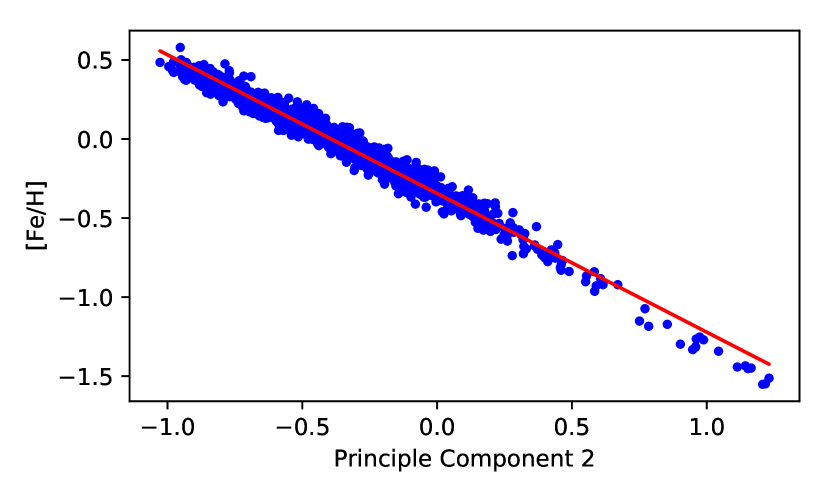
Figure 1: Metallicity against the second principal component from the PCA. A linear regression line is shown in red, highlighting that the correlation between the principal component and the APOGEE metallicity is well described by a linear fit.

With the metallicity principal component identified, we ran an iterative process to reduce the number of input parameters so that the resulting calibration was not over determined. The process is as follows: the decomposition was completed with the 84 colour index combinations addressed earlier, and the combination with the weakest contribution to the second principal component was removed. The decomposition was then performed again with $n-1$ dimensions, repeating the process until the tightest correlation with the fewest parameters remained. At this point, removing another colour index contribution would greatly impact the correlation with APOGEE metallicity.

At the end of this procedure, we found that the best colour indices to use were a linear combination of the $u-b$ index from the Strömgren photometric system and the $(G-K)^{2}$ index combining the $G$ band from Gaia’s photometry and the $K$ band from 2MASS. A second round of PCA was conducted with these two indices, as well as the APOGEE metallicity itself, resulting in a linear calibration of the form

$$\text{[Fe/H]}_{\text{cal}}=a_{0}(G-K)^{2}+a_{1}(u-b)+a_{2}$$ (2)

This calibration still had some residual trends, particularly in the $G-K$ colour index. To correct this, we further fitted a 5th order polynomial in $G-K$ to the residuals and subtracted this from the metallicity calibration in Equation 2. This polynomial was derived from adding terms to the residual fit until the trend was flattened by eye within the scatter. Hence, our final calibration was of the form:

$$\begin{split}\text{[Fe/H]}_{\text{cal}}&=c_{1}(G-K)^{5}+c_{2}(G-K)^{4}+c_{3}(G-K)^{3}\\ &+c_{4}(G-K)^{2}+c_{5}(G-K)+c_{6}(u-b)+c_{7}\end{split}$$ (3)

with calibration parameters:

$$c_{1} =-0.346793 c_{2} =3.108458$$

$$c_{3} =-10.38798 c_{4} =15.35047$$

$$c_{5} =-10.86391 c_{6} =1.729865$$

$$c_{7} =0.875089$$

Our calibration into the $G-K$ vs $u-b$ plane is shown in the upper panel of Fig. 2, where stars are colour coded by their APOGEE metallicity. Also shown in the bottom panels is the residual of our photometric metallicity calibration as function of spectroscopic [Fe/H] and $G-K$. The standard deviation of the residuals (shown in red) is 0.18 dex. Again we note that for [Fe/H] $\lesssim-1$, our calibration systematically overestimates the true metallicity, as seen in the APOGEE [Fe/H] residual plot. However, this is of little concern for the sake of our study, since the bulk of planets lie well above this limit.

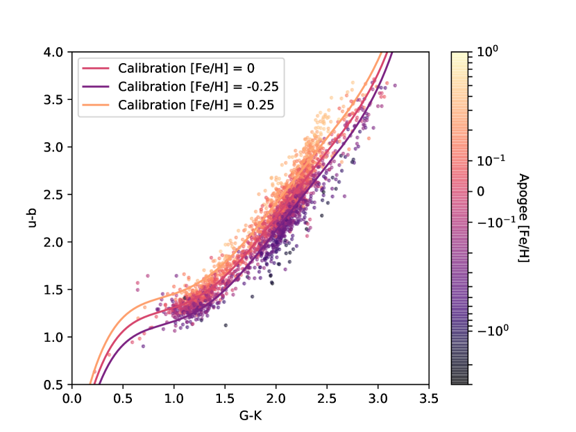
(a)

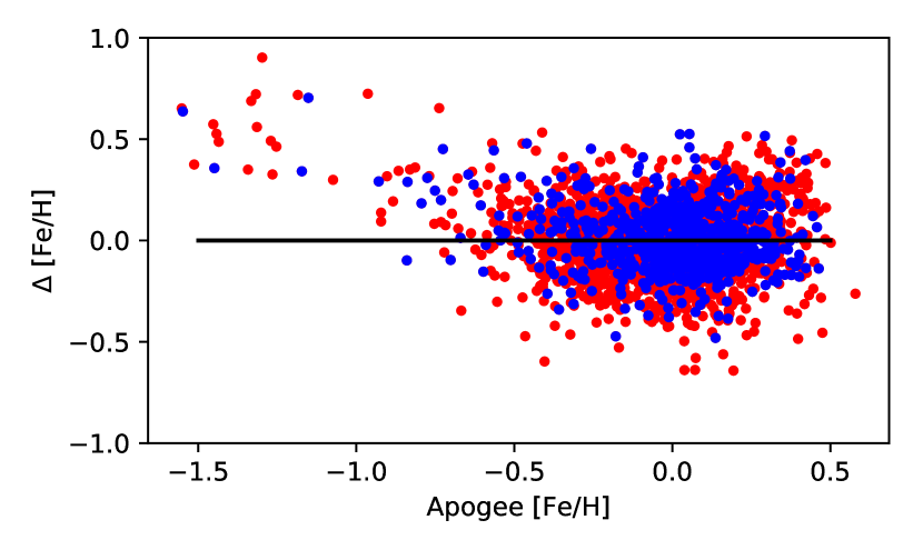
(b)

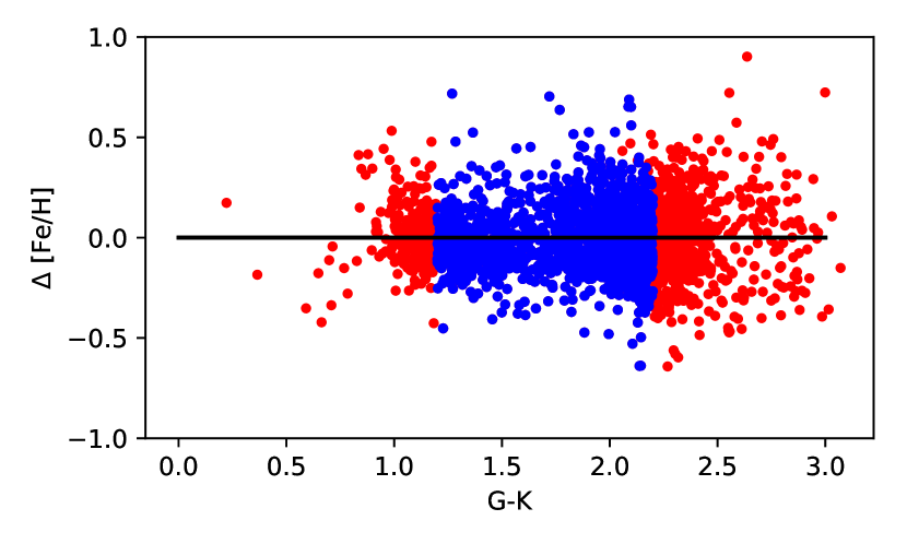
(c)

Figure 2: Comparison of our photometric metallicity calibration against that of APOGEE. a) The $G-K$, $u-b$ colour plane coloured by the APOGEE [M/H] metallicity index. Our photometric metallicity calibration is shown by the lines for a given metallicity. b) Metallicity residuals (our metallicity - APOGEE) against APOGEE metallicity. Red plots the full catalogue of stars, whereas blue only plots stars that fall within the colour cut discussed in the text. c) Same as b, but against the $G-K$ colour index.

Especially when looking at the $G-K$ residual plot, we can see by eye that this calibration does not hold well everywhere. As we will describe in the following section, we performed multiple colour and magnitude cuts to determine a selection for which the sample of KOI host stars is representative of the larger KIC population, as well as such that the metallicity callibration is well behaved. We determined that this range is:

$$1.4\leq u-b\leq 2.8$$

$$1.2\leq G-K\leq 2.0$$

The residuals for the colour cut are shown in blue in Fig. 2, with a smaller standard deviation of 0.16 dex.

Figure 3: Comparison of our photometric metallicity against that of Petigura et al. (2017) and Furlan et al. (2018), with residuals plotted against the literature values of metallicity, effective temperature and surface gravity.

To test the validity of the calibration, our photometric metallicities were tested against the spectroscopic metallicities measured by Petigura et al. (2017) and Furlan et al. (2018). It should be noted that these samples comprise of mostly main-sequence stars; the regime where most planet host stars reside. The comparisons are shown in Fig. 3, with a mean difference (Our metallicity - Petigura et al. (2017)) of $-0.05\pm 0.14$ dex, and (Our metallicity - Furlan et al. (2018)) of $0.00\pm 0.10$ dex. Both of these are well within the quoted uncertainty of our metallicity calibration. There is an indication that the scatter increases towards cooler $T_{\rm{eff}}$ and higher $\log(g)$. As spectroscopic parameters are harder to determine for cooler stars, the increased scatter could be due to deficiencies in our calibration sample, as well as in the spectroscopic samples we compare against.

4 Determining a Representative Sample

When using a sample to perform population studies, it is important to assess how well such a sample is representative of the underlying population of stars in the field. In this case, the underlying population of stars in the Kepler field is that assembled through the KIC catalogue, whereas our population inferences are derived using the KOI sample (note that in both cases a cross-match against Gaia and Strömgren photometry is required, see discussion in Section 2). For e.g., in comparing the metallicity distribution of the KOI sample to the KIC sample, it is important to understand the extend of any differences in brightness or colour distributions between the two samples, as this could bias conclusions about planetary demographics. If the KIC sample were to be extend to fainter magnitudes, it would trace stars further away in the Galaxy, and differences in metallicity with respect to the KOI would also stem from Galactic metallicity gradients (e.g., Boeche et al., 2013; Mikolaitis et al., 2014). Likewise, if the KIC sample were to extend to bluer colours, it would encompass early-type, young stars whose metallicities span a limited range, reflecting the chemistry of the present day ISM (e.g., Nieva & Przybilla, 2012; Luck, 2017). If however the KIC and KOI samples are very similar in apparent magnitude and colour distributions, we can perform a meaningful comparison between their metallicities.

Since our sample is drawn from photometric catalogues, we can perform well defined magnitude and colour cuts and ensure the KOI sample represents the underlying sample of stars found in the KIC catalogue. This is different from spectroscopically selected samples, where stars are picked for their KOI status at the time observations are done, and often favouring brighter targets. For example, in the California-Kepler Survey (Petigura et al., 2017), spectroscopy was obtained for KOI brighter than $14.2$, with fainter targets appended for a variety of reasons. In contrast, with a photometric sample is straightforward to observe stars to a given magnitude limit, regardless of how the Kepler planet catalogue grows in size with time.

To derive colour and magnitude cuts for the KIC and KOI samples, we applied the methodology described in Casagrande et al. (2016), who used it to build an unbiased sample of asteroseismic targets in the Kepler field. We started by taking the full sample of KOI, and benchmark their distribution in $(G-K)$ and $(u-b)$ colours, as well as apparent $G$ magnitudes against the KIC sample in the same ranges. To this purpose we used the Kolmogorov-Smirnov (KS) statistic on the colour and magnitude distributions. The significance levels between the KOI and the KIC sample pass from being virtually zero when stars are selected regardless of their colours and magnitudes, to order 20 to 70 percent when using the cuts listed below:

$$1.4\leq u-b\leq 2.8$$

$$1.2\leq G-K\leq 2.0$$

$$14.1\leq G\leq 16.0$$

This implies that the null assumption that the two samples are drawn from the same population cannot be rejected. These cuts were determined by exploring different ranges and each time running a KS test. We checked that similarly high percentages were also obtained if using a different diagnostic such as the Wilcoxon rank-sum test. Other colour combinations were also explored, although we focus our discussion on $(G-K)$ and $(u-b)$ since these indices underpin our metallicity calibration. The results are summarised in Table 1, and were repeated for the subset of KOIs that have a confirmed disposition according to the NASA Exoplanet database (Table 2). In the following of the paper the full photometric catalogue will be referred to as the parent population when restricted to the above colour and magnitude ranges, and its comparison aginst the KOI and confirmed KOI is shown in Fig. 4.

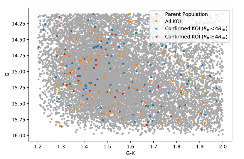
Figure 4: Comparison between the full photometric catalog and KOI (all and confirmed) observed over the same sky footprint.

Table 1: KS statistic, Wilcoxon rank-sum statistic and resulting p-values of the distribution of colours and magnitudes between all KOIs and the full photometric sample when the cuts discussed in Section 4 are applied.

Parameter	KS Statistic $D$	KS $p$	Wilcoxon Statistic $U$	Wilcoxon $p$
$G-K$	0.047	0.667	0.408	0.683
$u-b$	0.053	0.499	0.798	0.424
$G$	0.043	0.756	0.217	0.828

Table 2: KS statistic, Wilcoxon rank-sum statistic and resulting p-values of the distribution of colours and magnitudes between all confirmed KOIs and the full photometric sample when the cuts discussed in Section 4 are applied.

Parameter	KS Statistic $D$	KS $p$	Wilcoxon Statistic $U$	Wilcoxon $p$
$G-K$	0.061	0.714	0.233	0.671
$u-b$	0.091	0.233	-1.575	0.115
$G$	0.062	0.709	0.425	0.816

5 Obtaining Radii and Masses

One trend we aimed to investigate was the “Planet-Radius gap”, a feature where there is a relative absence of planets with radii around 1.9 $R_{\oplus}$ (e.g., Owen & Wu, 2013; Fulton et al., 2017), with some studies showing that the depression follows a slight dependence on the mass of the host star (e.g., Fulton & Petigura, 2018; Berger et al., 2020b).

We derived stellar masses and radii using the Bayesian isochrone fitting algorithm Elli (Lin et al., 2018), which is built upon the MIST isochrones (Choi et al., 2016). The input parameters used by Elli are effective temperatures ($T_{\rm{eff}}$), 2MASS $K$ magnitudes, reddening, Gaia DR2 parallaxes, surface gravities $\log(g)$ and our photometric metallicities. In the following, we describe in detail our procedure.

To obtain effective temperatures we run the InfraRed Flux Method (IRFM) for all our KOIs. The IRFM is an almost model independent photometric technique originally devised to obtain angular diameters to a precision of a few per cent, and capable of competing against intensity interferometry should a good flux calibration be achieved (e.g., Blackwell & Shallis, 1977; Blackwell et al., 1980). We used the implementation described in Casagrande et al. (2020) which employs Gaia and 2MASS photometry to derive effective temperatures and angular diameters for stars of known metallicity and surface gravity. We adopted our photometric metallicities, and $\log(g)$ from the KOI catalogue. Effective temperatures derived from the IRFM were then fed into Elli along the other parameters needed to derive stellar radii and masses. A new estimate of $\log(g)$ was computed, iterating between the IRFM and Elli. Because of the mild dependence of the IRFM on the adopted metallicity and surface gravity (see e.g., Alonso et al., 1995; Casagrande et al., 2006) only a couple of iterations were necessary to converge on a final mass and radius for each star.

First, we compared our $T_{\rm{eff}}$ against those published in Petigura et al. (2017) and Furlan et al. (2018), showing excellent agreement, with a mean difference of 30 K and a standard deviation of 90 K (Fig. 5). Since $T_{\rm{eff}}$ from the IRFM are sensitive to reddening (where a change of $\pm 0.01$ in $E(B-V)$ has an impact of $\pm 50$ K), this comparison suggests that reddening is well under control.

In addition to stellar radii obtained from isochrone fitting, the availability of angular diameters from the IRFM and Gaia distances (Bailer-Jones et al., 2018) for all our targets allowed us to derive radii independently of stellar isochrones. We dub these "empirical radii" since they are virtually free from any stellar modelling assumption. Since distance uncertainties propagate into radii, from now on we apply a very mild cut on parallax uncertainty to remove stars with clearly ill measured parallaxes. At the same time, we do not want to apply any stringent parallax requirement, as this could potentially introduce an extra sample selection effect. We only require stars to have parallaxes better than 20 percent, but in fact the vast majority of our targets have distances determined at a few percent level. Finally, the planet radius was determined by applying the planet to star radius ratio provided in the KOI catalogue; a parameter estimated from the transit depth.

Fig. 6 shows the relative difference between the stellar radii derived from Elli and the empirical ones –(Elli radius - empirical radius)/Elli radius– with a a mean of $0.00\pm 0.03$ solar radii, and a standard deviation of 2 percent. This gives confidence that the radii and other stellar quantities derived from Elli are robust and that possible systematic differences arising from our methodology are within our quoted uncertainties. From this point on, we adopt the empirical radii as our accepted stellar radii.

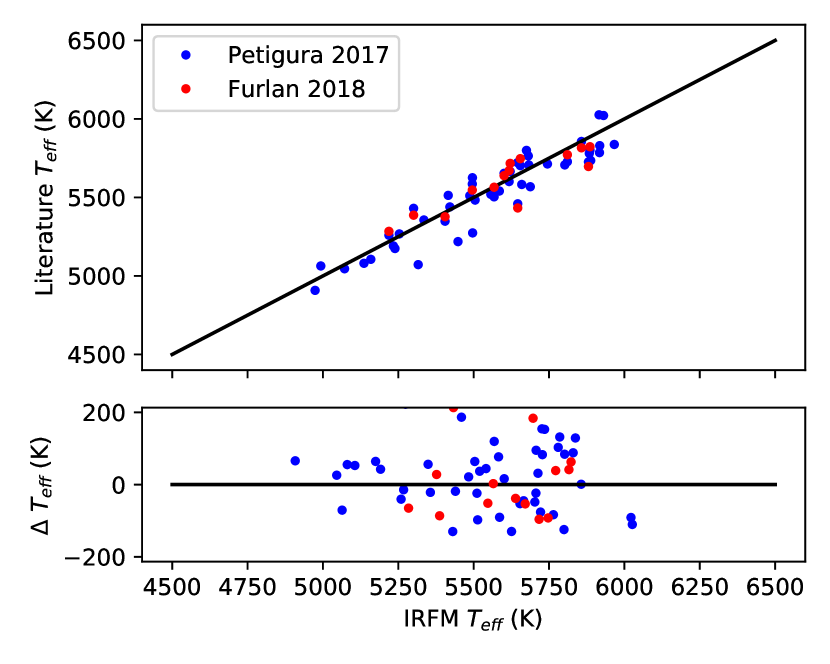
Figure 5: Comparison of our effective temperatures from the IRFM (abscissa) with those of Petigura et al. (2017) and Furlan et al. (2018).

The empirical radii also have good relative uncertainties, with a mean of 3.4 percent, which is on par with that of Berger et al. (2020a) and Fulton & Petigura (2018). When multiplied by the Kepler planet to star radius ratio, we find our planet radii have uncertainties with a mean of 6.2 percent, highlighting that uncertainties in the Kepler radius ratio carry a significant contribution to the uncertainties in the planetary radius.

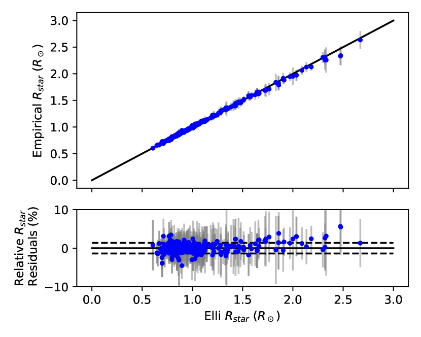
Figure 6: Comparison of the stellar radii derived from Elli against the empirical ones obtained using the Bailer-Jones et al. (2018) distances and angular diameters from the IRFM. Uncertainties are shown in grey, with dashed lines indicating 1$\sigma$ scatter.

Finally, we tested our stellar parameters against those derived by Berger et al. (2020a), in particular the stellar luminosity (Fig. 7) and stellar radius (Fig. 8). Both of these parameters had extremely good agreement, with luminosity residuals of $-1\pm 7~{}\%$ and radius residuals of $0.4\pm 2.6~{}\%$; any trends within these residuals are less than the order of these uncertainties. We also tested our masses against their catalogue, finding a mean difference and standard deviation of $-6\pm 7$ percent, which again shows good agreement albeit with our masses tending to be lower than those of Berger et al. (2020a).

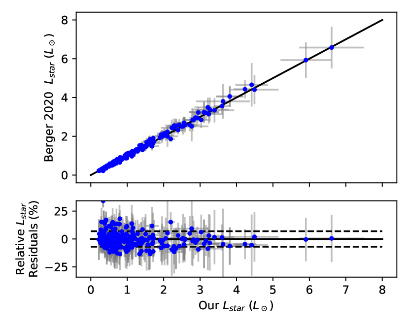
Figure 7: Comparison of our stellar luminosities with those of Berger et al. (2020a). Uncertainties are shown in grey, with dashed lines indicating 1$\sigma$ scatter.

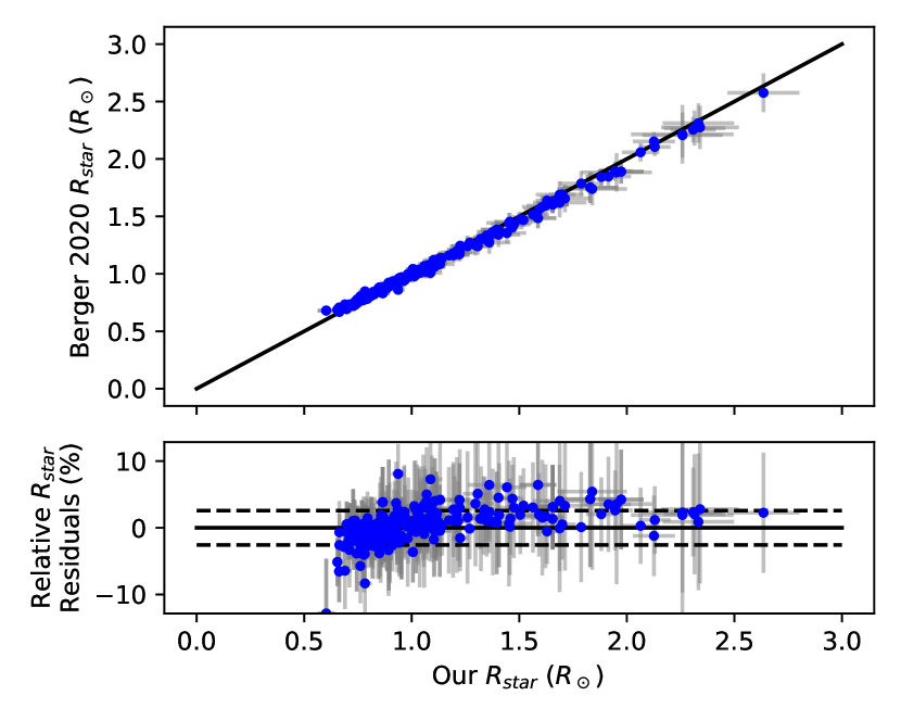
Figure 8: Comparison of our stellar radii with those of Berger et al. (2020a). Uncertainties are shown in grey, with dashed lines indicating 1$\sigma$ scatter.

6 Results and Analysis

6.1 Metallicity trends

We first investigated trends concerning metallicity between the KOI host stars and the parent population (ref. Section 4). The subset of KOIs which have been labelled as confirmed by the NASA Exoplanet Database was also extracted and compared, before finally splitting the confirmed KOIs between large ($R_{p}\geq 4R_{\oplus}$) and small ($R_{p}<4R_{\oplus}$) planetary radii. The use of the confirmed sub-sample was to ensure that we were not affected by non-planetary companions, with the trade off of a smaller sample size. If a star had multiple planets, then it was classified according to the radius of the largest one. We note here that our sample mainly consists of sub Neptunes and super Earths with radii between 1 and 10 $R_{\oplus}$, along with a few larger and smaller exoplanets. Histograms and cumulative distribution functions (CDFs) of these populations are shown in Fig. 9.

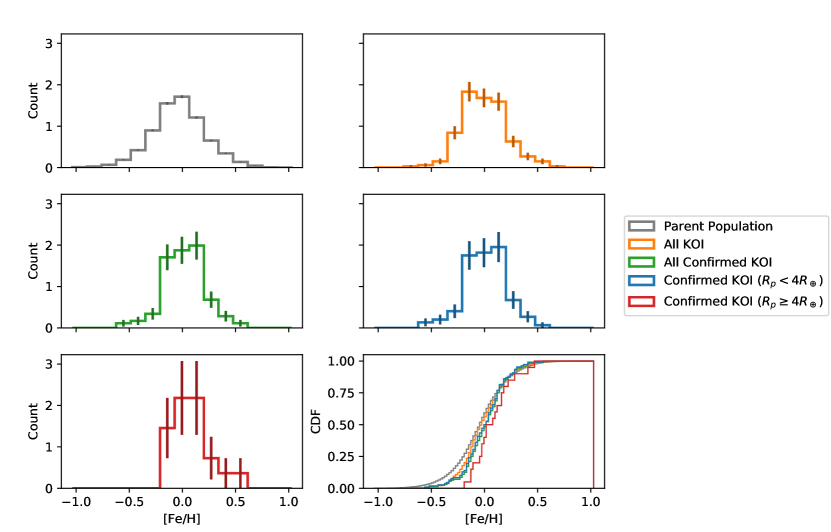
Figure 9: Histograms and cumulative distribution functions of the metallicity distribution of various exoplanet subsets. Histograms are normalised with an area of one. Confirmed KOI are those with a NASA Exoplanet Database designated disposition of confirmed, whereas “All KOI” refer to those with a disposition of confirmed or candidate.

The mean metallicity of the KOIs ([Fe/H] = -0.01) and especially that of the confirmed KOIs ([Fe/H] = 0.02) is different from that of the parent population of stars as a whole ([Fe/H] = -0.03). This suggests that the exoplanet host stars are more metal rich than the rest of the candidate KOIs. To confirm this deviation, KS and Wilcoxon rank-sum tests were undertaken using the full metallicity distribution function (MDF), with each subset being tested against the parent population. The results are shown in Table 3.

Table 3: KS tests of the metallicities of the different subsets against the metallicies of the full photometric sample in the same colour and magnitude ranges.

Sample	KS Statistic $D$	KS $p$	Wilcoxon Statistic $U$	Wilcoxon $p$
All KOI host stars	0.081	0.087	-1.629	0.103
All confirmed KOI host stars	0.155	0.004	-2.879	0.004
Confirmed KOI ($R_{p}<4R_{\oplus}$)	0.141	0.025	-2.112	0.035
Confirmed KOI ($R_{p}\geq 4R_{\oplus}$)	0.308	0.035	-2.389	0.017

With a $p\simeq$ 9 percent, the null hypothesis that the MDF of all KOI is drawn from that of the parent population cannot be rejected. However, when restricting ourselves to the sample of confirmed KOIs, the $p$ value drops to a mere $0.4$ percent, thus allowing us to reject the null hypothesis at a very high significance. This is also the case for the two sub-samples with small and large planetary radii, where we can reject the null hypothesis at the 5% significance level. In particular, when looking at the histograms in Fig. 9, we see that the confirmed exoplanet host stars seem to favour higher metallicities than their non-exoplanet hosting counterparts, supporting earlier results (e.g., Gonzalez, 1997; Santos et al., 2004; Fischer & Valenti, 2005; Zhu, 2019). The larger p-value from the sample of all KOIs (including those with a disposition of candidate), may be due to some of the candidate KOIs not being planetary companions.

To investigate further the trend with metallicity, a plot of the percentage of stars with a confirmed KOI for a given metallicity bin was created. This particular diagram was based on the work of Zhu (2019), and can be seen in Fig. 10. Also plotted in this figure is the percentage of stellar systems with multiple exoplanets, with the aim to compare to the findings by Brewer et al. (2018) as to whether multiple exoplanet systems were preferentially around lower metallicity host stars.

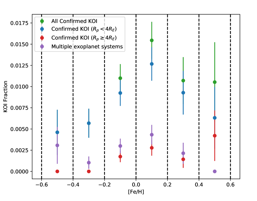
Figure 10: Fraction of the parent population that host exoplanets for a given metallicity bin. Different colours refer to the different planet sizes of the KOI, or whether they are present in a system with multiple objects. Error bars are drawn from the Poisson statistic.

As predicted from Santos et al. (2004), Fischer & Valenti (2005) and Zhu (2019) among others, and as inferred from the cumulative distribution function, exoplanets (and especially those that have a radius greater than 4 Earth radii) appear to form preferentially around higher metallicity stars. Smaller exoplanets also appear to favour higher metallicities, peaking above solar metallicity, and then declining at very high metallicities although in our case the significance of this trend is only at 1 $\sigma$ level and so it should be considered carefully. This furthers the work of Buchhave et al. (2012), who claims that while smaller exoplanets form around stars with a wide range of metallicities, large exoplanets form around primarily metal rich stars. We show that while the smaller exoplanets have a weaker trend than their larger counterparts, they still have a bias towards metallicities around and above solar metallicity.

We summarise these findings in Table 4, which shows the percentage of stars in our representative sample of the Kepler field that host exoplanets for metallicities above and below solar metallicity. Here, to almost 2$\sigma$ significance we find that large exoplanets are more than twice as likely to be found around metal rich stars while smaller exoplanets are 1.5 times as likely. We thus find that all exoplanets are more likely to be observed at higher metallicities, with the size of the exoplanet influencing the strength of this trend.

Multiple planet systems also have a peak at solar metallicity. The upward trend in the lowest metallicity bin while intriguing has a too large uncertainty to allow any meaningful comparison with Brewer et al. (2018), who found that compact multi-planet systems occur more frequently around stars of increasingly lower metallicities.

Table 4: Percentage of stars in our representative sample of the Kepler field hosting KOIs for high ([Fe/H] $\geq$ 0) and low ([Fe/H] < 0) metallicities. Uncertainties are drawn from the Poisson statistic.

Sample	Metal Poor [Fe/H] < 0 (%)	Metal Rich [Fe/H] > 0 (%)
All confirmed KOI host stars	0.88 $\pm$ 0.12	1.37 $\pm$ 0.16
Confirmed KOI ($R_{p}<4R_{\oplus}$)	0.77 $\pm$ 0.11	1.12 $\pm$ 0.15
Confirmed KOI ($R_{p}\geq 4R_{\oplus}$)	0.11 $\pm$ 0.04	0.25 $\pm$ 0.07
Multiple exoplanet systems	0.24 $\pm$ 0.06	0.33 $\pm$ 0.08

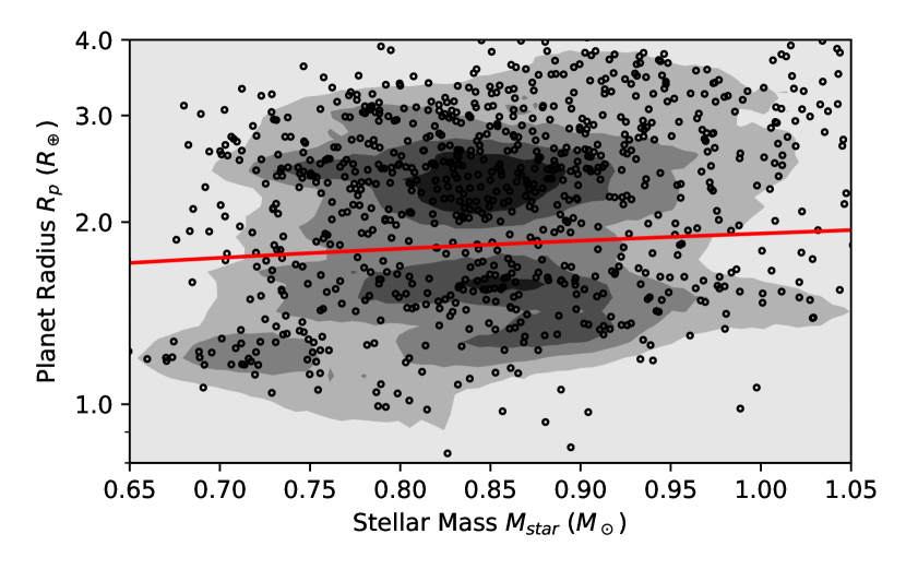
Figure 11: 2D Monte Carlo distribution of the stellar mass and planetary radius of KOI with a confirmed disposition. Density contours are shown behind a random selection of 1000 samples. Note the presence of a gap around $R_{p}=1.9\,R_{\oplus}$. Also plotted in red is the best fit line to the radius gap from Berger et al. (2020b), with their slope of $d\log{R_{p}}/d\log{M_{star}}=0.26$. It can be seen that our data also fits this line well, showing that the radius gap has a slight positive correlation with stellar mass.

6.2 The planet-radius gap

As mentioned previously, one aim of this work was to study the planet-radius gap. With the stellar mass and planet radius we recovered through the processes outlined in Section 5, we generated a 2D density plot through a Monte Carlo (MC) simulation. We drew 10,000 samples assigning each time normal errors in stellar mass and planet radius for each of our confirmed KOI data points, and plotted the density distribution as contours in Fig. 11. We also plot 1000 random samples from the MC simulation. We chose not to include the KOIs with a candidate disposition due to the potential presence of false positives in this sample (examined in Section 6.1).

The contour levels suggest the presence of a gap around 1.8-2.0 $R_{\odot}$, with a mild positive slope as function of stellar mass. This trend has been found in previous works by Fulton & Petigura (2018) and Berger et al. (2020b). Indeed, if in Fig. 11 we overplot the best fit line to the radius gap from Berger et al. (2020b) (slope $d\log{R_{p}}/d\log{M_{star}}=0.26$), this line also cuts across our gap.

To view the gap more clearly, we contracted this plot over mass and normalised the data, creating a simple histogram of planet radii. This is shown in solid red in Fig. 12. We also show in solid blue the histogram of planet radii when KOI with a disposition of candidate are included. The most notable feature is a very clear bimodal distribution, with a gap again at 1.9 $R_{\oplus}$, supporting the conclusions of e.g Fulton & Petigura (2018) and Berger et al. (2020b). The restriction of only including confirmed KOI influences the distribution by increasing the side of the second peak at $\sim 2.5~{}R_{\oplus}$ and decreasing the width of the first at $\sim 1.6~{}R_{\oplus}$, but the location of the gap does not change.

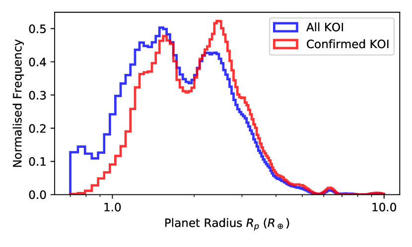
Figure 12: Normalised histograms of the planetary radius of all KOI (blue) and only the confirmed KOI (red).

Following the work of Berger et al. (2020b), we also looked at how the radius histogram was affected by the incident stellar flux falling on the planet. We chose the separating flux value of 150 $F_{\oplus}$ from Berger et al. (2020b), to test to see whether we identified a similar trend; our sample had 114 planets designated as cool. This is plotted in Fig. 13, where again we have chosen to only plot confirmed KOI. We recover that planets with higher incident flux exhibit smaller radii than their cooler counterparts, possibly due to evaporation of the atmospheres of these planets. As with Berger et al. (2020b), we caution that these results may be a result of small number statistics and are likely fraught with Kepler selection effects.

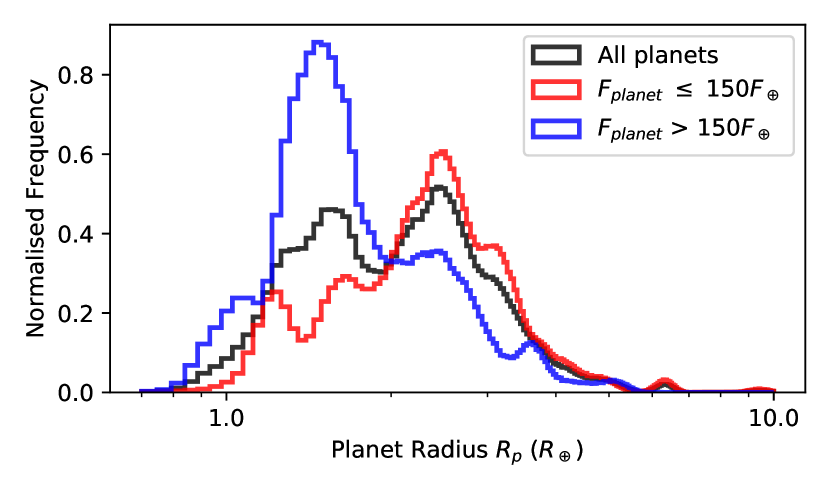
Figure 13: Normalised histograms of the planetary radius of confirmed KOI, separated by host star luminosities. All confirmed KOI are shown in black, whereas the red and blue histograms represent the subset with a planetary flux of less than and greater than 150 $F_{\oplus}$ respectively.

7 Conclusions

We have compiled a photometric catalogue of stars in the Kepler field utilising photometry from Gaia, Strömgren and 2MASS catalogues. We created a metallicity calibration based on APOGEE spectroscopy to obtain a metallicity for our photometric sample, and then performed well defined colour and magnitude cuts to ensure our dataset was a representative sample of the underlying population of stars. We then derived temperatures and angular diameters using the IFRM, which were then used to derive stellar radii and stellar mass through Bayesian isochrone fitting. The resultant parameters were compared favourably with previous results from the literature, especially giving stellar radii with relative uncertainties around 3.4 percent. Planetary radii uncertainties of 6.2 percent hence indicate a major uncertainty contribution from the Kepler planet to star ratio.

The main purpose of this work has been to outline a methodology to derive photometric stellar parameters for planet host stars. The advantage of using photometry is that it allows a better control of sample selection effect, and in the future we believe to more robust inferences on population studies. Although our sample is currently relatively small, especially compared to recent studies such as that of Fulton & Petigura (2018) and Berger et al. (2020b), we are able to recover a number of known trends.

We find that the stars hosting confirmed KOIs have a statistically different metallicity distribution than the parent population of stars in the Kepler field. We also find that this statistical claim is not valid for the sample of KOIs that include those with a disposition of candidate, consequences of potential undetected false positives in the list of KOIs.

We quantify the metallicity distribution differences between KOI and the larger sample of KIC stars, finding that KOI hosts tend to be more metal rich than their non-planet hosting counterparts. While holding especially true for large exoplanets larger than $4~{}R_{\oplus}$, which has been known about in literature for some time (e.g, Buchhave et al., 2012), we also find this holds for smaller exoplanets albeit to a weaker extent. This follows the conclusions of (e.g, Zhu, 2019).

We recover the planet radius gap at $\sim 1.9~{}R_{\oplus}$. We also tentatively find that there is a trend that planets with a high incident flux (>150 $F_{\oplus}$) tend to have smaller radii.

The major reason for our limited sample size is due to the number of stars in the Kepler field for which we had Strömgren photometry for. However, we anticipate that with the upcoming Gaia DR3 release we can obtain a larger sample of e.g., Strömgren photometry (or other suitable metallicity sensitivity indices) directly from the $BP$ and $RP$ spectra. With this larger sample, we believe that the methods described in this paper will be limited solely by Kepler uncertainties, thus allowing for more robust statistics and deeper insight into the demographics of Kepler’s exoplanet population.

Data Availability

The data underlying this article are available in the article and in its online supplementary material.

References

- Abolfathi et al. (2018) Abolfathi B., et al., 2018, ApJS, 235, 42
- Alonso et al. (1995) Alonso A., Arribas S., Martinez-Roger C., 1995, A&A, 297, 197
- Arce & Goodman (1999) Arce H. G., Goodman A. A., 1999, ApJ, 512, L135
- Bailer-Jones et al. (2018) Bailer-Jones C. A. L., Rybizki J., Fouesneau M., Mantelet G., Andrae R., 2018, AJ, 156, 58
- Batalha et al. (2010) Batalha N. M., et al., 2010, ApJ, 713, L109
- Berger et al. (2020a) Berger T. A., Huber D., van Saders J. L., Gaidos E., Tayar J., Kraus A. L., 2020a, AJ, 159, 280
- Berger et al. (2020b) Berger T. A., Huber D., Gaidos E., van Saders J. L., Weiss L. M., 2020b, AJ, 160, 108
- Bessell (2005) Bessell M. S., 2005, ARA&A, 43, 293
- Blackwell & Shallis (1977) Blackwell D. E., Shallis M. J., 1977, MNRAS, 180, 177
- Blackwell et al. (1980) Blackwell D. E., Petford A. D., Shallis M. J., 1980, A&A, 82, 249
- Boeche et al. (2013) Boeche C., et al., 2013, A&A, 559, A59
- Borucki et al. (2010) Borucki W. J., et al., 2010, Science, 327, 977
- Brewer et al. (2018) Brewer J. M., Wang S., Fischer D. A., Foreman-Mackey D., 2018, ApJ, 867, L3
- Brown et al. (2011) Brown T. M., Latham D. W., Everett M. E., Esquerdo G. A., 2011, AJ, 142, 112
- Bruntt et al. (2012) Bruntt H., et al., 2012, MNRAS, 423, 122
- Buchhave et al. (2012) Buchhave L. A., et al., 2012, Nature, 486, 375
- Casagrande & VandenBerg (2014) Casagrande L., VandenBerg D. A., 2014, MNRAS, 444, 392
- Casagrande & VandenBerg (2018) Casagrande L., VandenBerg D. A., 2018, MNRAS, 479, L102
- Casagrande et al. (2006) Casagrande L., Portinari L., Flynn C., 2006, MNRAS, 373, 13
- Casagrande et al. (2010) Casagrande L., Ramírez I., Meléndez J., Bessell M., Asplund M., 2010, A&A, 512, A54
- Casagrande et al. (2014) Casagrande L., et al., 2014, ApJ, 787, 110
- Casagrande et al. (2016) Casagrande L., et al., 2016, MNRAS, 455, 987
- Casagrande et al. (2019) Casagrande L., Wolf C., Mackey A. D., Nordland er T., Yong D., Bessell M., 2019, MNRAS, 482, 2770
- Casagrande et al. (2020) Casagrande L., et al., 2020, arXiv e-prints, p. arXiv:2011.02517
- Choi et al. (2016) Choi J., Dotter A., Conroy C., Cantiello M., Paxton B., Johnson B. D., 2016, ApJ, 823, 102
- Cloutier & Menou (2020) Cloutier R., Menou K., 2020, AJ, 159, 211
- Fischer & Valenti (2005) Fischer D. A., Valenti J., 2005, ApJ, 622, 1102
- Fulton & Petigura (2018) Fulton B. J., Petigura E. A., 2018, AJ, 156, 264
- Fulton et al. (2017) Fulton B. J., et al., 2017, AJ, 154, 109
- Furlan et al. (2018) Furlan E., et al., 2018, ApJ, 861, 149
- Gaia Collaboration et al. (2018) Gaia Collaboration et al., 2018, A&A, 616, A1
- Ginzburg et al. (2018) Ginzburg S., Schlichting H. E., Sari R., 2018, MNRAS, 476, 759
- Gonzalez (1997) Gonzalez G., 1997, MNRAS, 285, 403
- Gupta & Schlichting (2020) Gupta A., Schlichting H. E., 2020, MNRAS, 493, 792
- Hardegree-Ullman et al. (2020) Hardegree-Ullman K. K., Zink J. K., Christiansen J. L., Dressing C. D., Ciardi D. R., Schlieder J. E., 2020, ApJS, 247, 28
- Huber et al. (2014) Huber D., et al., 2014, ApJS, 211, 2
- Kunder et al. (2017) Kunder A., et al., 2017, AJ, 153, 75
- Lin et al. (2018) Lin J., Dotter A., Ting Y.-S., Asplund M., 2018, MNRAS, 477, 2966
- Lopez & Rice (2018) Lopez E. D., Rice K., 2018, MNRAS, 479, 5303
- Luck (2017) Luck R. E., 2017, AJ, 153, 21
- Majewski et al. (2017) Majewski S. R., et al., 2017, AJ, 154, 94
- Mikolaitis et al. (2014) Mikolaitis Š., et al., 2014, A&A, 572, A33
- Molenda-Żakowicz et al. (2013) Molenda-Żakowicz J., et al., 2013, MNRAS, 434, 1422
- Nieva & Przybilla (2012) Nieva M. F., Przybilla N., 2012, A&A, 539, A143
- Owen & Wu (2013) Owen J. E., Wu Y., 2013, ApJ, 775, 105
- Owen & Wu (2017) Owen J. E., Wu Y., 2017, ApJ, 847, 29
- Petigura (2020) Petigura E. A., 2020, AJ, 160, 89
- Petigura et al. (2017) Petigura E. A., et al., 2017, AJ, 154, 107
- Santos et al. (2004) Santos N. C., Israelian G., Mayor M., 2004, A&A, 415, 1153
- Schlafly & Finkbeiner (2011) Schlafly E. F., Finkbeiner D. P., 2011, ApJ, 737, 103
- Schlegel et al. (1998) Schlegel D. J., Finkbeiner D. P., Davis M., 1998, ApJ, 500, 525
- Skrutskie et al. (2006) Skrutskie M. F., et al., 2006, AJ, 131, 1163
- Van Eylen et al. (2018) Van Eylen V., Agentoft C., Lundkvist M. S., Kjeldsen H., Owen J. E., Fulton B. J., Petigura E., Snellen I., 2018, MNRAS, 479, 4786
- Zhu (2019) Zhu W., 2019, ApJ, 873, 8