Affinity, kinetics, and pathways of anisotropic ligands binding to hydrophobic model pockets

Abstract

Using explicit-water molecular dynamics (MD) simulations of a generic pocket-ligand model we investigate how chemical and shape anisotropy of small ligands influences the affinities, kinetic rates and pathways for their association to hydrophobic binding sites. In particular, we investigate aromatic compounds, all of similar molecular size, but distinct by various hydrophilic or hydrophobic residues. We demonstrate that the most hydrophobic sections are in general desolvated primarily upon binding to the cavity, suggesting that specific hydration of the different chemical units can steer the orientation pathways via a ‘hydrophobic torque’. Moreover, we find that ligands with bimodal orientation fluctuations have significantly increased kinetic barriers for binding compared to the kinetic barriers previously observed for spherical ligands due to translational fluctuations. We exemplify that these kinetic barriers, which are ligand specific, impact both binding and unbinding times for which we observe considerable differences between our studied ligands.

Molecular recognition in aqueous solution is of fundamental importance in living and chemically engineered systems. As an example, enzymes bind a substrate to an often complementary, concavely shaped binding site Kim et al. (1997). Also, receptors are activated or inhibited if their binding pockets take up a small molecule, such as a neurotransmitter Creese et al. (1976), a hormone Borngraeber et al. (2003) or a pharmaceutical drug Teixeira-Clerc et al. (2006). Moreover, this binding principle from nature is copied in chemical engineering of supramolecular chemistry, where so-called cavitands Hillyer et al. (2016); Wanjari et al. (2016) or macrocycles Xue et al. (2012) are designed as molecular containers. The superior principle is often pictured by a binding agent representing a ’key’ or ’guest’ selectively fitting into a complementary shaped ’lock’, or ’host’, respectively, giving the names of key-lock or host-guest principles Koshland (1995); Hu et al. (2009). Modern drug screening and design is based on this principle.

Key-lock binding in water exhibits strong solvent-mediated effects which in fact can be diverse Ball (2008) but are very often of hydrophobic nature. By today, it is well accepted from computer simulations and experimental studies that hydrophobic protein pockets comprise strong contributions to the binding affinity of ligands through non-trivial dehydration effects Young et al. (2007, 2010); Nair et al. (1991); Carey et al. (2000); Setny et al. (2009, 2010); Baron et al. (2010). Motivated by the recent recognition of the importance of drug-receptor binding rates for the efficacy of the drug Pan et al. (2013), most novel studies have now added on the role of water in hydrophobic association kinetics. In particular, Setny et al. Setny et al. (2013) documented a direct coupling between water fluctuations in hydrophobic pockets and the ligand binding rate. Using explicit-water MD simulations, they studied the binding of a spherical ligand to a hydrophobic pocket represented by a hemispherical surface recess in a model wall Setny and Geller (2006); Setny (2007, 2008). They demonstrated that hydrophobically driven wet-dry fluctuations inside the pocket could lead to locally enhanced ligand friction and kinetic barriers in the vicinity of the binding site. These findings were consistent with observations of Berne and coworkers in a study on a similar hydrophobic key-lock model setup Mondal et al. (2013). In a most recent work of ours Weiß et al. (2017), we also showed that increased hydrophobicity by modulating shape or water affinity of the pocket influences the friction peak and can speed up the binding kinetics.

All previous modeling work on hydrophobic pocket-ligand binding exclusively focused on simple spherical ligands, mimicking a methane-like molecule Setny et al. (2009, 2010); Baron et al. (2010); Setny et al. (2013); Setny and Geller (2006); Setny (2007, 2008); Weiß et al. (2017) or other idealized carbon-based assemblies Mondal et al. (2013); Tiwary et al. (2015); Tiwary and Berne (2016). Chemical and shape anisotropy of ligands, however, are of fundamental importance for biological function Ludwig et al. (2007); Wittmann and Strasser (2017). For instance, analyses of a series of chemical derivatives demonstrated that altering the ensemble of ligand binding orientations changes signaling output, providing a novel mechanism for titrating allosteric signaling activity Bruning et al. (2010). Other work found that only the orientation of the substrates correlated with the conjugation capacity in in-vitro experiments, where the conjugation reaction proceeded only when the hydroxyl group of the ligand is oriented towards the coenzyme Takaoka et al. (2010). Hence, the widely used spherical models of ligands is most of the time inadequate for the identification of potential binding pockets in computational methods Benkaidali et al. (2013). A more systematic investigation of the effects of chemical and shape anisotropy of a ligand to a hydrophobic pocket on affinity as well as kinetics is therefore of high fundamental interest. Since complex anisotropic ligands have more degrees of freedom than a simple sphere, interesting behavior in the coupling to hydration and in the association pathways can be expected, possibly opening more opportunites in drug design.

So far, fundamental studies on solvent-influenced binding pathways of anisotropic substrates can be only found in more coarse-grained descriptions discussing the role of solvent depletion in molecular pair association processes. Kinoshita Kinoshito (2004), for instance, calculated the depletion potential of two freely rotating plates which favors an association pathway with very tilted orientations to each other. Moreover, Roth et al. Roth et al. (2002) estimated the association potential of a rod associating to a planar wall. They found that solvent depletion generates a torque that will favor an equivalently tilted association pathway. Also in the application to key-lock models König et al. (2008) with a spheroidal ligand the depletion forces were calculated and found to exhibit comparably high barriers if the ligand faces the pocket with its extended side during the association process. In essence, they conclude that an aspherical ligand will non-parallely associate to a concave binding site and only in the last step fold/lay down into the pocket. Dlugosz et al. Długosz and Antosiewicz (2016) studied the binding time in Brownian simulations of an spheroidal ligand that electrostatically associated to a concave pocket. If the hydrodynamic interactions were turned off, the mean binding time was faster than in calculations which considered hydrodynamic interactions. Hence the water-mediation, i.e., hydrodynamics, plus the reorientation process of the aspherical ligand increased the absolute binding time.

In this paper, we investigate how chemical and shape anisotropy of small ligands influence the affinities, kinetic rates and pathways for the association to hydrophobic binding sites using explicit-water MD simulations of the generic pocket model used previously Setny et al. (2009, 2010); Baron et al. (2010); Setny et al. (2013); Setny and Geller (2006); Setny (2007, 2008); Weiß et al. (2017). We highlight in particular how water influences the binding and the unbinding of various aromatic ligands to hydrophobic binding sites, and how the new rotational degrees of freedom couple to our previously reported water fluctuation effects Setny et al. (2013); Weiß et al. (2016, 2017). First, we focus on the binding of benzene to a hydrophobic planar wall compared to a hydrophobic binding pocket and present the ligand reorientation potential, pathway, and friction profile. We elaborate on an interpretation of enhanced friction as kinetic barrier in a rescaled energy landscape which was originally introduced by Hinczewski et al. Hinczewski et al. (2010) in the context of protein folding. Moreover, we discuss how the kinetic barrier varies upon our various ligands, which are all of similar molecular size, but distinct by various hydrophilic or hydrophobic residues. We describe that the general concept of a kinetic barrier is not only influenced by the previously reported water fluctuations but also by the new rotational degree of freedom of the ligands. We analytically discuss the impact of the resulting slowdown and see that the most significant implications must follow for the unbinding process, whereas the unbinding time can be influenced by hundreds of microseconds. Thus the kinetic barrier can be steered by ligand shape and, in turn, steer the binding and unbinding rates such that the action of a toxin and the efficacy of a drug can be optimized.

I Methods

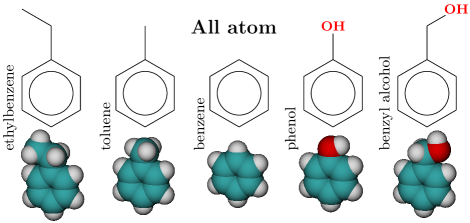
Figure 1: All ligands studied in this work contain an aromatic ring. The reference benzene ring in the center is alkylated with a methyl and ethyl group, respectively, while stepping to the left creating toluene and ethylbenzene. Stepping to the right, a hydroxyl group and a hydroxymethyl moiety are respectively introduced to form phenol and benzyl alcohol.

I.1 Varyious non-spherical ligands

In contrast to our previous study Weiß et al. (2017) in which we modified the physicochemical properties of the binding site, we investigate here the binding of various aromatic compounds to hydrophobic binding sites. Therefore we use ethylbenzene, toluene, benzene, phenol and benzyl alcohol, which are illustrated in Fig. 1. The aromatic compounds are represented by the OPLS-AA force field Jorgensen et al. (1996) whereas we employ the LINCS algorithm to constrain all bond lengths. Phenol can be considered to be the most hydrophilic compound based on its ratio of polar to non-polar solvent-accessible surface area while hydrophobicity increases for the ligands left and right from it in Fig. 1. We use the TIP4P model for water Jorgensen et al. (1983); Jorgensen and Madura (1985).

I.2 Constrained simulations for PMF and ligand orientation

The simulation setup is illustrated in Fig. 2 and 3 which is the same as in our previous study Weiß et al. (2017). The ligand binding process is constrained to one-dimensional diffusion along $z$, the distance of the ligand center-of-mass perpendicular to the pocketed wall shown in Fig. 2 and 3. Movement of the center of mass (COM) along $x$- and $y$-direction was strongly restrained with a harmonic potential with spring constant $k_{x/y}=42000\leavevmode\nobreak\ \text{kJ\leavevmode\nobreak\ mol}^{-1}\leavevmode\nobreak\ \text{nm}^{-2}$. To probe selected observables as functions of the ligand separation to the binding site we utilized umbrella sampling simulations along $z$. In each umbrella setup, the center of mass of the ligand was constrained to a given position $z_{i}$ using an external harmonic potential with spring constant $K=835\leavevmode\nobreak\ \text{kJ\leavevmode\nobreak\ mol}^{-1}\leavevmode\nobreak\ \text{nm}^{-2}$. We define the origin $z=0$ by the first layer of the wall that is in contact with the water (Fig. 2) or the pocket’s bottom, namely the inner crystal layer of the pocket (Fig. 3). The first umbrella potential was placed at $z=3.14\leavevmode\nobreak\$Å. Up to 48 additional umbrella windows with 0.5 Å spacing were introduced to cover increasing ligand-pocket distances. The individual umbrella simulations produced 10 ns with a step size of 2 fs, while the ligand coordinate was stored for every time step and the water coordinates were stored every 20 fs. The potential of mean force (PMF) was obtained by the weighted histogram analysis method (WHAM) Kumar et al. (1992); Zhu and Hummer (2012).

The molecular snapshots in Figs. 2 and 3 also illustrate how we define the ligand orientation by the angle $\theta$. It is the angle between the normal vector of the aromatic ring and the $z$-axis, and consequentially the angle between the ring’s plane spanned by its ring atoms and the $x$-$y$-plane (gray), which is the parallel plane to the wall. Note that $\theta$ runs from 0 (parallel to the $x$-$y$ plane) to $\pi/2$ (perpendicular to $x$-$y$ plane) given the molecule’s ring symmetry and thus its otherwise degenerate orientations, such as 0 and $\pi$. We sample the distribution of $\theta$ in each umbrella window and hence its Boltzmann inversion, the angular potential $W(\theta,z)$. Note, that the distribution must be normalized by the $2$sin$(\theta)$ scaling to calculate $W(\theta,z)$.

The additional residue breaks the ring symmetry which we assumed for the benzene ring. Therefore, we formally replace our angular coordinate $\theta$ by a new angle $\phi$. It defines the angle between the respective residue R and the $z$-axis as illustrated in the upper sketch of Fig. 4. Note that the unique mapping onto $\phi$ ranges from $0$ to $\pi$, which is the necessary descriptor range to distinguish all orientations of the ligands other than benzene. If the angle is zero the residue points into the water, away from the pocket. If the angle is equal to $\pi$ the residue points into the pocket, away from the bulk. These two orientations are degenerate for the benzene ring and the definition of $\theta$, as mentioned above. We sample the potential $U(\phi,z)$ from the orientation distributions in all umbrella windows in the same way we obtained the potential $W(\theta,z)$. Note, that the distributions must be normalized by the sin$(\phi)$ scaling to calculate $U(\phi,z)$.

I.3 Unconstrained simulations for mean first passage times

For each setup, we store a production run of 20 ns in steps of 0.2 ps in which the ligand is constrained at the reflective boundary at $z=22$ Å for the planar binding site and $z=29$ Å for the pocketed binding site. This initial trajectory served as a source for randomly seeded initial configurations for subsequent binding event simulations. We then sampled more than a thousand binding events starting from independent, initial frames by randomly picking one from the previously generated production run. To ensure a selection’s randomness, upon possible re-selection, we applied an additional annealing step: within a short simulation of 50 ps, the configuration was heated up to 350 K in a stochastic integrator scheme. After this, the heated simulation was equilibrated for 100 ps at 298 K using the Berendsen thermostat and the Velocity Verlet algorithm. In the final production run the ligand was released, free to move along the $z$-direction. The runs were terminated once the ligand bound to the binding site at $z=4$ Å. The time for binding, that is, the first passage time (FPT), was then averaged to calculate the mean first passage time (MFPT) $\mathcal{T}(z,z_{f})$, the time the ligand takes to bind from $z$ to the final bound position $z_{f}=4$ Å. The curves for $\mathcal{T}(z,z_{f})$ are discussed in the SI.

In simple cases, the MFPT curve can be theoretically calculated using a Markovian approach for diffusion in one dimension. Given an energy landscape $V(z)$ such as a PMF and a possibly spatially dependent friction $\xi(z)$, the MFPT can be calculated by Weiss (1967); Siegert (1951)

$$\mathcal{T}(z,z_{f})=\beta\int_{z_{f}}^{z}\mathrm{d}z^{\prime}\xi(z^{\prime})\mathrm{e}^{\beta V(z^{\prime})}\int_{z^{\prime}}^{z_{\mathrm{max}}}\mathrm{d}z^{\prime\prime}\mathrm{e}^{-\beta V(z^{\prime\prime})}\,.$$ (1)

where $z_{f}$ and $z_{\mathrm{max}}$ denote an absorbing and reflective boundary, respectively. We exploit and elaborate on the framework of Eq. (1) in section B, C, and D.

II Results

II.1 Ligand reorientation

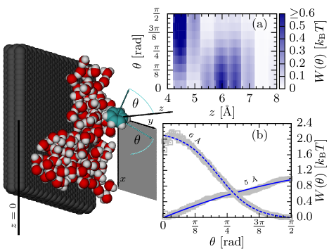
Figure 2: The simulation snapshot illustrates benzene, the planar wall and part of the water. The binding process is constrained to one-dimensional diffusion along $z$. The ligand’s orientation is quantified by the angle $\theta$ between the atomic plane of the ring atoms and the $x$-$y$ plane (gray). It is the same angle like the one between the normal vector of benzene and the $z$-axis. (a) The dependence of the angular potential $W(\theta,z)$ on $z$ illustrates the pathway upon binding. Here the transition from a favorably perpendicular ($\theta=\pi/2$) to a lateral ($\theta=0$) orientation for decreasing ligand-wall separations occurs on a narrow range from roughly $z=5\leavevmode\nobreak\ \mathrm{\AA}$ to $z=7\leavevmode\nobreak\ \mathrm{\AA}$. Panel (b) exemplifies sampled data for $W(\theta,z)$ as gray symbols including blue lined fits for $z=6\leavevmode\nobreak\$Å and $z=5$ Å. Strikingly the perpendicular orientation is favored by over $2\leavevmode\nobreak\ k_{\mathrm{B}}T$.

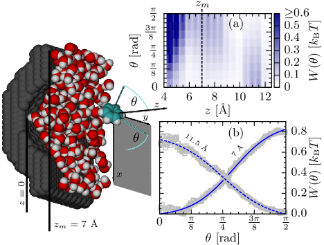
Figure 3: The simulation snapshot illustrates the benzene as ligand, a section of the hemispherical binding site and part of the water. The binding process is also constrained to one-dimensional diffusion along $z$. The pocket bottom is defined as origin $z=0$ such that the pocket mouth is around $z_{m}=7\leavevmode\nobreak\ \mathrm{\AA}$. (a) The dependence of the angular potential $W(\theta,z)$ on $z$ illustrates the pathway upon binding. For $z>10$ Å a perpendicular orientation to the wall (and towards the water interface) is energetically favored whereas for $z<10$ Å it aligns with the pocket bottom and the $x$-$y$-plane. Panel (b) exemplifies sampled data for $W(\theta,z)$ as gray symbols including blue lined fits for $z=11.5\leavevmode\nobreak\$Å and $z=7$ Å.

We first study the reference ligand, i.e., benzene associating to a planar hydrophobic wall. Fig. 2 (a) and (b) draw the orientation potential $W(\theta,z)$ from umbrella sampling. Benzene undergoes a clear orientation pathway which depends on the ligand separation to the wall. While the ligand is at $z=6$ Å the perpendicular orientation for $\theta=\pi/2$ is energetically favored by a little more than $2\leavevmode\nobreak\ k_{\mathrm{B}}T$. The example of $W(\theta,z)$ for $z=6$ Å is shown in Fig. 2 (b) where the gray symbols represent the simulation sampled data, and the dashed blue line is a fit of a shifted hyperbolic tangent. Thus at these ligand separations to the wall benzene partly desolvates if it orients perpendicularly to the $x$-$y$ plane. Proceeding to smaller $z$ values aligning parallel/lateral to the wall ($\theta=0$) is favored because of steric repulsion with the wall. The example data (gray symbols) and fit (solid blue line) of the angular potential for $z=5\leavevmode\nobreak\$Å are again shown in Fig. 2 (b).

We now turn to binding to the hydrophobic pocket. In Fig. 3 (a) and (b) we see that the benzene association to the pocketed binding site is qualitatively similar, but the reorientation from perpendicular to lateral occurs on a much broader range in $z$. While the ligand is $10--12$ Å away from the pocket bottom, it favors the perpendicular orientation. It is actually only slightly favored by little more than half a $k_{\mathrm{B}}T$ at $z=11.5$ Å, as Fig. 3 (b) exemplifies. At even closer distances such as $z=7$ Å benzene favors the lateral orientation by more than half a $k_{\text{B}}T$ as shown in panel (b). Hence, benzene favorably aligns with the pocket bottom before it enters the pocket (compare Fig. 3 (a) again).

We conclude that binding of benzene to our hydrophobic binding sites involves an energetically favored, perpendicular orientation which is possibly disadvantageous since the final bound configuration requires parallel alignment. For slit-like binding sites, this could be advantageous if a ligand must enter perpendicularly before binding. We suppose that the orientation pathway is steered by water and thus solvation free energy of the ligand because the molecule can partly desolvate while orienting out of the water interface. In the case of a hemispherically molded binding site, the smeared water interface allows even earlier desolvation and reorientation upon binding which, on top, energetically weakens the perpendicular orientation.

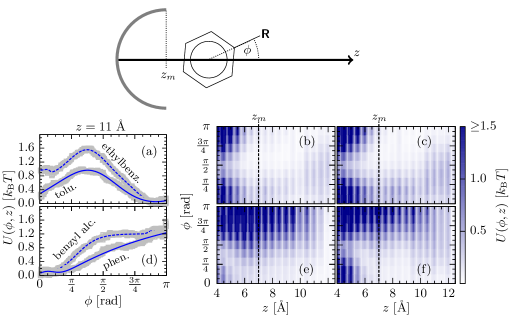
Figure 4: The upper sketch schematically represents the pocket and ligand connected by the $z$-axis. Also the pocket mouth $z_{m}=7\leavevmode\nobreak\ \mathrm{\AA}$. The angle $\phi$ is taken to be the angle between the respective ligand’s residue R and the $z$-axis. Plot (a) shows two examples for the angular potentials $U(\phi,z=11\leavevmode\nobreak\ \mathrm{\AA})$ from umbrella sampling of ethylbenzene (dashed) and toluene (solid). (The gray symbols plot the sampled data and the blue lines represent smooth interpolation functions.) The color map plots show the angular potentials from all umbrella windows for (b) toluene and (c) ethylbenzene. Panel (d) also shows the examples of $U(\phi,z=11\leavevmode\nobreak\ \mathrm{\AA})$ for benzyl alcohol (dashed) and phenol (solid). For (e) phenol and (f) benzyl alcohol we also show the full angular potentials $U(\phi,z)$ as color map plots.

Additional observations on the reorientation pathways cover the association of our remaining aromatic compounds benzyl alcohol, phenol, toluene and ethylbenzene to the pocketed binding site only. All of these ligands comprise an aromatic ring onto which an additional residue is attached such as the hydroxyl group to phenol.

In Fig. 4 (a) two examples are shown for $U(\phi,z)$ where ethylbenzene and toluene were constrained at $z=11$ Å. Both exhibit a barrier around $\phi=3\pi/8$, whereas the barrier is smaller in the case of toluene. This behavior seems to be very significant for these two aromatic compounds which comprise an alkyl residue. Hence, if these ligands are at intermediate positions they partly solvate either the aromatic ring (minimum at $\phi=\pi$) or the alkyl group (minimum at $\phi=0$). Both of these orientations yield an energetic gain over an unfavored tilted orientation around $\phi=3\pi/8$. Nevertheless, $\phi=\pi$ is globally favored because the aromatic ring yields higher energetic contributions from the electrostatic energy from its partial charges. Fig. 4 (b) and (c) show that the bimodal orientations of toluene and ethylbenzene range from $z=12\leavevmode\nobreak\$Å to $9$ Å. Overall the orientation pathway funnels along angles that are larger than $\pi/2$ such that the solvation of the aromatic ring stays favored, however, the ligand samples all orientations. Finally, in the bound state around $z=4\leavevmode\nobreak\ \mathrm{\AA}$, ethylbenzene and toluene are sterically hindered to take orientations other than $\phi\approx\pi/2$.

The orientation pathway is again very different for phenol and benzyl alcohol. In Fig. 4 (d) the potentials $U(\phi,z=11\leavevmode\nobreak\ \mathrm{\AA})$ for benzyl alcohol and phenol exhibit a favored orientation for $\phi=0$. Both of these ligands have polar residues which contain a hydroxyl group. These impose two potential hydrogen bonding sites: the oxygen and the associated hydrogen atom. As a consequence, the favorable solvation of the hydroxyl group yields a strong orientation to $\phi=0$. This angle is even more favored at closer distances $z$, such that the barrier around $\phi=\pi$ increases to several $k_{\text{B}}T$. In Fig. 4 (e) and (f) for phenol and benzyl alcohol, respectively, one can see that the energy to take an almost perpendicular orientation exceeds the $1.5\leavevmode\nobreak\ k_{\mathrm{B}}T$ plotted scale. Overall these plots make evident that benzyl alcohol and phenol favorably solvate their hydroxyl groups while they approach the pocket. Finally both ligands orient to $\phi=\pi/2$ in the bound state ($z=4\leavevmode\nobreak\ \mathrm{\AA}$). In summary, the orientation of all ligands suggests that their pathways are driven by solvation free energy such that the parts which have the highest energetic costs upon hydration are primarily desolvated.

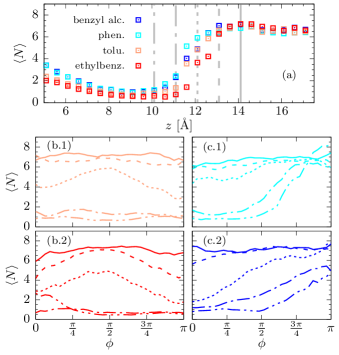
Figure 5: Panel (a) shows the dewetting transition of the pocket plotting the average pocket water occupancy against ligand distance to the pocket for benzyl alcohol, phenol, toluene, and ethylbenzene. The gray vertical lines serve as the legend to the reference positions that are used as line styles in the remaining figure panels. Panel (b.1) and (b.2) plot $\langle N\rangle$ against ligand orientation $\phi$ for toluene and ethylbenzene, respectively, at the indicated positions in panel (a). Panel (c.1) and (c.2) plot the same $\langle N\rangle$ dependence for phenol and benzyl alcohol, respectively. Note, that while a given ligand’s hydroxyl group orients towards the pocket, the otherwise dewetted binding site can be considerably hydrated.

In turn, we observe how ligand position and orientation influence the pocket dewetting. Fig. 5 plots the average pocket water occupancy $\langle N\rangle$ against the two spatial descriptors position $z$ and angle $\phi$ for ethylbenzene, toluene, phenol, and benzyl alcohol. The transition from wet to dry occurs while a given ligand is at $z=10$ Å to $z=15$ Å as shown in Fig. 5 (a). An average of six to seven pocket water molecules transition to less than an average of one while the ligand is still in front of the pocket at $z=10$ Å. If the ligand enters the pocket this minimum pocket water occupancy increases again up to three to four water molecules which fit into the pocket if the ligand is bound around $z=5$ Å. Additionally, comparing the dewetting transition for instance of ethylbenzene and phenol, we see that more elongated and hydrophobic ligands induce the dewetting farther away. Further, the vertical gray lines indicate the reference positions for which we observe how $\langle N\rangle$ depends on the ligand orientation in panels (b.1), (b.2), (c.1), and (c.2) for toluene, ethylbenzene, phenol, and benzyl alcohol, respectively. In panels (b.1) and (b.2), toluene and ethylbenzene pronouncedly induce dewetting if either elongated edge, the aromatic or residue group, reach towards the pocket and, thus, increase the hydrophobic confinement at $\phi=\pi$ or $\phi=0$. In contrast, phenol and benzyl alcohol enhance pocket wetting if their polar residue is oriented towards the pocket, which essentially pushes the associated solvation layers into the pocket. Hence the hydroxyl groups can considerably hydrate an otherwise dewetted pocket if they are oriented toward it.

II.2 Dissipative forces and kinetic barriers

Previously we discussed that the pocket water density fluctuations yield additional dissipative forces that slow the binding Setny et al. (2013); Weiß et al. (2016, 2017). Firstly, pocket water occupancy fluctuations and ligand friction were shown to couple Setny et al. (2013). The long time transients of the water fluctuations lead to long time transients in the ligand’s force correlations, and for small ligand separations to the pocket, the water fluctuations increase due to the increased confinement. Secondly, we derived that the hydration fluctuation time scale and the ligand friction directly couple by a proportional relation Weiß et al. (2016). In this context, we found that a bimodal nature of hydration fluctuations is sufficient to enhance the ligand friction prior to association to the pocket. And finally, we demonstrated that results from ligand constraining simulations must be corrected by the time transients which occur in unconstrained simulations. Only then one can capture the non-Markovian properties, i.e. long-time correlations, for accurate kinetic predictions. We obtain the dissipative forces and time transients (memory) in a friction profile calculated via Hinczewski et al. (2010)

$$\beta\xi^{\mathrm{M}}(z)=\frac{\partial\mathcal{T}(z)}{\partial z}\frac{\mathrm{e}^{-\beta V(z)}}{\int_{z}^{z_{\mathrm{max}}}\mathrm{d}z^{\prime}\mathrm{e}^{-\beta V(z^{\prime})}}$$ (2)

where the PMF $V(z)$ and the MFPT curve $\mathcal{T}(z,z_{f})$ are employed. Hence, we can combine the results from ligand constraining simulations, i.e., the PMF, and unconstrained simulations, i.e., the MFPT. We denote this profile by $\xi^{\mathrm{M}}(z)$ accounting for the Markovian assumption of Eq. (2). Still, we know from our previous work that this profile non-trivially incorporates the non-Markovian memory effects by our MFPT input. Rigorously speaking, we shall not consider $\xi^{\mathrm{M}}(z)$ as friction profile Setny et al. (2013); Weiß et al. (2016, 2017). We refer to $\xi^{\mathrm{M}}(z)$ as the kinetic profile which can be incorporated in a rescaled free energy landscape capturing all kinetic effects, whereas we follow the lines of Hinczewski et al. Hinczewski et al. (2010).

Fig. 6 (a.1) and (a.2) show $\xi^{\mathrm{M}}(z)/\xi_{{}_{\infty}}$ whereas we normalize by the respective bulk friction constant to compare our various ligands. The values of the bulk friction values are analyzed and discussed in the SI. For example, the kinetic profile of benzene binding to the wall can be well assumed to be constant. Moreover, if benzene binds to the pocket, the dominant feature of the steady-state friction $\xi^{\mathrm{M}}(z)$ is a Gaussian peaking structure, which we will model and fit by

$$\xi(z)=\xi_{\infty}+\Delta\xi\mathrm{e}^{-(z-z_{p})^{2}/\sigma^{2}}\,\,\,.$$ (3)

Thus, the peak height $\Delta\xi$, position $z_{p}$ and width $\sigma$ define a peak that adds to the bulk friction constant $\xi_{\infty}$. This peak roots from pocket hydration fluctuations as we also previously discussed for binding of a spherical ligand to the same pocket Weiß et al. (2017) which we replot here as gray circles. The key to the additional dissipative forces are the bimodal wet-dry hydration fluctuations which couple to the ligand. In comparison to the data for the spherical ligand, the dissipative forces for benzene peak wider and shift slightly further into the bulk by roughly half an Å  which makes their tail reach to $z\sim 11$ Å. This well coincides with the position where the perpendicular orientation is favored (see Fig. 3 (a)). Hence, benzene is exposed to the increasing friction at larger $z$-values because it reaches with its extended side towards the fluctuating interface.

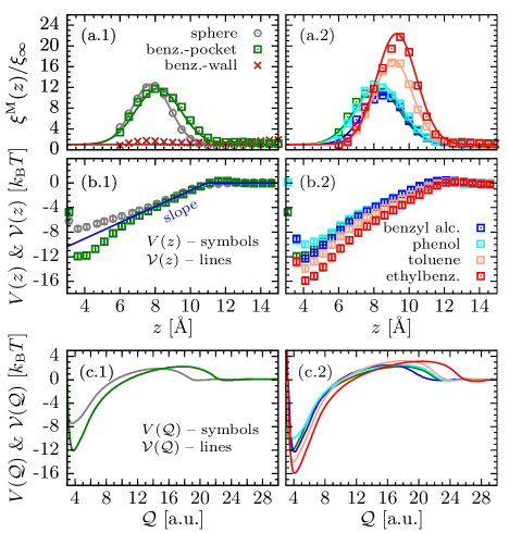
Figure 6: (a.1) The kinetic profiles from Eq. (2) exhibit peaks if benzene (green squares) and the spherical ligand (gray circles) bind to the pocketed site. If benzene binds to the wall (red crosses) the friction can be well assumed constant. The respectively colored lines represent Gaussian function fits from Eq. (3). (a.2) Comparably peaking profiles can be observed for our remaining aromatic compounds, whereas those of ethylbenzene and toluene are even more enhanced. Panels (b.1) and (b.2) show the original PMF $V(z)$ as colored symbols. Note that the original PMFs of benzene and the spherical ligand binding to the pocket share the similar attracting slope (blue line) which sets in around $z=11$ Å. Panels (c.1) and (c.2) show the rescaled energy landscapes $\mathcal{V}(\mathcal{Q})$ as lines which exhibit the additional kinetic barrier along the rescaled coordinate.

The kinetic profiles for the remaining aromatic compounds ethylbenzene, toluene, phenol and benzyl alcohol are shown in Fig. 6 (a.2) where they are compared to the replotted profile of benzene. The compounds phenol and benzyl alcohol are extended by a hydroxyl group and a methanol group, respectively, thus offering polar patches. Their size is elongated compared to the benzene ring; however, their kinetic profiles match the one of benzene, i.e., their kinetic barriers well coincide. Since the orientation pathways of these two ligands dominantly expose the aromatic ring to the pocket, the hydration fluctuations yield a similar kinetic profile.

Ethylbenzene and toluene are purely hydrophobic compounds made up of a conjugated carbon ring that is extended by an ethyl and a methyl group, respectively. Their kinetic profiles are more enhanced and reach further into the bulk. For these two ligands, the peak is even higher and hints that it contains contributions other than the bimodal pocket hydration. We suggest that the additionally bimodally fluctuating orientation adds to the peak of the kinetic profile. In essence, binding of these two ligands involves two degrees of freedom, which bimodally fluctuate and which thus can both add to additional dissipative forces in our one-dimensional description. More importantly the peak positions for ethylbenzene and toluene shift farther away from the pocket. In comparison to benzene these ligands are even longer and are subject to the hydration fluctuations farther outside the pocket.

To judge the impact of the kinetic profiles we rescale it into an effective free energy landscape. We choose a new reaction coordinate $\mathcal{Q}=\mathcal{Q}(z)$, as suggested by Hinczewski et al. Hinczewski et al. (2010), such that in the new coordinates the friction is scaled to the constant value $1\leavevmode\nobreak\ k_{\mathrm{B}}T\leavevmode\nobreak\ \mathrm{ns}\leavevmode\nobreak\ \mathrm{nm}^{-2}$. Then the rescaled coordinate is determined by $\mathcal{Q}^{\prime}=\mathrm{d}\mathcal{Q}/\mathrm{d}z=\sqrt{\xi^{\mathrm{M}}(z)/\xi_{{}_{\infty}}}$ and the PMF must be consistently rescaled such that

$$\begin{split}\mathcal{V}(\mathcal{Q}(z))&=V(z)+(\beta)^{-1}\mathrm{ln}(\mathcal{Q}^{\prime}(z))\\ &=V(z)+(2\beta)^{-1}\mathrm{ln}(\xi^{\mathrm{M}}(z)/\xi_{{}_{\infty}})\end{split}$$ (4)

In panels (c.1) and (c.2) we plot the rescaled potentials against the new coordinate $\mathcal{Q}$. The rescaled energy landscapes exhibit additional kinetic barriers which naturally origin from the kinetic profiles. The rescaled coordinate is calculated as the integral over $\sqrt{\xi^{\mathrm{M}}(z)/\xi_{{}_{\infty}}}$ such that the integration of the Gaussian shaped peak stretches the reaction coordinate. In comparison to the case for the spherical ligand (gray line), the peak in the kinetic barriers for the aromatic compounds (colored lines) shift farther away from the pocket, namely to increasing values of $\mathcal{Q}$. In general, the farther the barrier shifts down the attracting slope, the smaller is its impact because the anyhow attracting slope diminishes the repulsive slope on the r.h.s. of the barrier. In other words, part of the repulsive slope of the kinetic barrier reaches across the onset of attraction which makes its effect more significant for a slowed association. This result is consistent with the MFPT data which we present in the SI, where benzene and other aromatic compounds bind slightly slower than the spherical ligand. The binding times of ethylbenzene and toluene are even slower than those of benzene. The binding speeds of phenol and benzyl alcohol, however, are similar to the binding times of benzene.

In sum, the size and nature of a ligand can shift and tune the dissipative forces and the resulting kinetic barriers in the $\xi^{\mathrm{M}}(z)$ profiles. So far we only discussed this qualitatively with a scientist’s intuition for the shapes of energy landscapes. In the following, we approach our arguments in a quantitative picture by which we explore the full range of the possible impact of the kinetic barrier.

II.3 Impact of Steady-State Friction

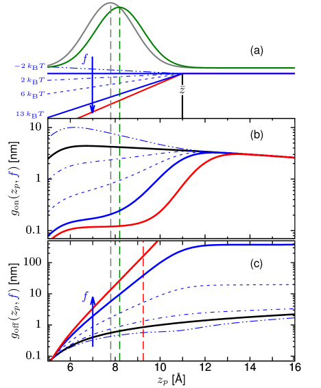
Figure 7: (a) The dominant features of the ligand binding process are the potential $V(z)=f(z-\bar{z})$ (blue), that strongly attracts the ligand given $z\leq\bar{z}$, and a Gaussian friction peak (gray and green) modeled by Eq. (3). Various other potential slopes are sketched as thin blue lines. (b) The factor $g_{\mathrm{on}}(z_{p},f)$ in Eq. (6) strongly depends on the friction peak position. While the negative shift $z_{p}-\bar{z}$ decreases, $g_{\mathrm{on}}(z_{p},f)$ and thus the impact of the friction peak decreases. Moreover turning to (even slightly) repulsive slopes $f$ drastically increases the impact of the kinetic barrier (double dotted dashed). (c) The factor $g_{\mathrm{off}}(z_{p},f)$ for the unbinding process exponentially increases with friction peak position $z_{p}$ and the repulsive slope $f$. In the example of ethylbenzene (red curve), the potential slope is the steepest, and the friction peak position lies farthest outside the pocket which is why the scaling factor is on the order of $\mathcal{O}(10^{2})$.

We already formalized the kinetic profile $\xi^{\mathrm{M}}(z)$ by its dominant feature the fitted Gaussian peak from Eq. (3) (see also Fig. 6). The common and dominant feature of the PMF is its significantly attracting slope with roughly $f=13\leavevmode\nobreak\ k_{\mathrm{B}}T\leavevmode\nobreak\ \mathrm{nm}^{-1}$ (see blue line in Fig. 6 (b.1)). Thus in the following minimalistic model we use $V(z)=f(z-\bar{z})$ for $z\leq\bar{z}$ and $V(z)=0$ otherwise, such that $\bar{z}$ denotes the inset position of a constant attraction with strength $f$. For illustration the simplified potential and friction are plotted together in the upper sketch of Fig. 7. In particular, the contribution of the friction peak, i.e., the second summand on the r.h.s. of Eq. (3), to the binding time in Eq. (1) is given by

$$\Delta\mathcal{T}=\beta\Delta\xi\int_{z_{f}}^{z}\mathrm{d}z^{\prime}\mathrm{e}^{\beta V(z^{\prime})-\frac{(z^{\prime}-z_{p})^{2}}{\sigma^{2}}}\int_{z^{\prime}}^{z_{\mathrm{max}}}\mathrm{d}z^{\prime\prime}\mathrm{e}^{-\beta V(z^{\prime\prime})}$$ (5)

whereas the stepwise definition of $V(z)$ has yet to be evaluated.

Fixing $\bar{z}=11$ Å, $z_{f}=4$ Å,and $z_{\mathrm{max}}=29$ Å, leaves the bracket in the integral in Eq. 5 dependent on the friction peak position $z_{p}$, width $\sigma$ and the force constant $f$. We lay out the detailed integration steps in the Appendix A. The result simplifies to

$$\Delta\mathcal{T}=\frac{\sqrt{\pi}\sigma}{2}\beta\Delta\xi\cdot g_{\mathrm{on}}(z_{p},f)$$ (6)

the product of friction peak height, width and a scaling factor $g_{\mathrm{on}}(z_{p},f)$. For the moment we can neglect the dependence of $g_{\mathrm{on}}(z_{p},f)$ on $\sigma$ because the direct proportionality of $\Delta T\propto\sigma$ is the dominating peak width dependence for our values of $\sigma$. The factor $g_{\mathrm{on}}(z_{p},f)$ quantifies the impact of the friction peak on the binding time which is why we will also refer to it as the scaling factor.

If we choose the slope of $f=13\leavevmode\nobreak\ k_{\mathrm{B}}T\leavevmode\nobreak\ \text{nm}^{-1}$ from Fig. 6 (b.1), the scaling factor, shown as blue solid line in Fig. 7 (b), steeply increases with the peak position of the kinetic profile. The broken blue line types indicate how $g_{\mathrm{on}}(z_{p},f)$ increases with decreasing potential slope $f$ whereas the thick black line is the case for $f=0$. If the force constant even becomes repulsive the scaling factor increases drastically because the repulsive potential slope and the repulsive kinetic barrier add up. We find that the mean binding time is certainly affected by and thus proportional to the friction peak height $\Delta\xi$, although, the impact can drastically decrease if the peak shifts downward the attracting slope. For repulsive slopes the scaling can drastically dominate such that for our case the unbinding is dominantly affected.

The result of the scaling factor $g_{\mathrm{off}}$ for the unbinding process is determined by interchanging the integration boundaries $z_{max}$ and $z_{f}$ in Eq. (5). We exemplify the scaling factor for the unbinding in Fig. 7 (c). Generally, the scaling factors exponentially scale with force constant $f$. Especially for our linearly attractive potential, they scale with $g_{\mathrm{on}}\propto\mathrm{exp}(\beta f(\bar{z}-z_{f}))$ for the binding process and $g_{\mathrm{off}}\propto\mathrm{exp}(\beta f(z_{p}-\bar{z}))$ for the unbinding process. Thus for unbinding it takes values much larger than one, i.e., $\mathcal{O}(10^{1})$, where for the binding it takes values two orders of magnitude smaller, i.e., $\mathcal{O}(10^{-1})$. In the special case of ethylbenzene, the slope $f$ is the steepest and the friction peak is farthest away from the pocket. Hence, the scaling factor is on the order of $\mathcal{O}(10^{2})$ for ethylbenzene. See also red curve in Fig. 7 (c).

II.4 Unbinding

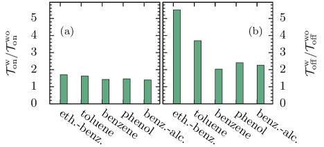
Figure 8: (a) The ratio of the average binding time with $\mathcal{T}_{\mathrm{on}}^{\mathrm{w}}$ and without $\mathcal{T}_{\mathrm{on}}^{\mathrm{wo}}$ kinetic barrier exhibits a constant impact during binding. (b) In contrast, the unbinding times dominantly increase by a factor of five in the ratio of the average unbinding times with $\mathcal{T}_{\mathrm{off}}^{\mathrm{w}}$ and without $\mathcal{T}_{\mathrm{off}}^{\mathrm{wo}}$ kinetic barrier.

In this section we want to compare the impact on average binding times

$$\mathcal{T}_{\mathrm{on}}=\frac{\int_{z_{\mathrm{b}}}^{z_{\mathrm{max}}}\mathrm{d}z^{\prime}\mathcal{T}(z^{\prime},z_{\mathrm{b}})}{(z_{\mathrm{max}}-z_{\mathrm{b}})}$$ (7)

where we choose the boundary to be bound as $z_{\mathrm{b}}=10$ Å, and the average unbinding times

$$\mathcal{T}_{\mathrm{off}}=\frac{\int_{z_{\mathrm{ub}}}^{z_{\mathrm{f}}}\mathrm{d}z^{\prime}\mathcal{T}(z^{\prime},z_{\mathrm{ub}})}{(z_{\mathrm{max}}-z_{\mathrm{ub}})}$$ (8)

where we choose the boundary to be unbound as $z_{\mathrm{ub}}=12$ Å. The boundary for binding is read from the kinetic barrier peak position. The boundary for the unbinding $z_{\mathrm{ub}}$ is chosen such that the unbinding process can be considered complete by overcoming the kinetic barrier. The respective MFPT curve $\mathcal{T}(z,z_{\mathrm{b/ub}})$ is calculated from Eq. (1) where the upper integration boundary is $z_{\mathrm{max}}$ for the binding case and $z_{f}$ for the unbinding case. For each ligand we choose two scenarios – one neglecting the kinetic barrier, thus $\xi(z)=\xi_{\infty}$ and one incorporating the kinetic barrier.

The histogram of Fig. 8 (a) plots the ratio $\mathcal{T}^{\mathrm{w}}_{\mathrm{on}}/\mathcal{T}^{\mathrm{wo}}_{\mathrm{on}}$ of the binding time with and without kinetic barrier. The barrier slows the binding time by a factor smaller than two for all ligands. In contrast, the average unbinding time is dominantly affected. We estimate that the kinetic barrier adds an extra $221\leavevmode\nobreak\ \mu$s to the unbinding time of ethylbenzene and less than $1\leavevmode\nobreak\ \mu$s to that of phenol. Moreover, the ratio of the average unbinding times with and without kinetic barrier in Fig. 8 (b) yields a factor of more than five for ethylbenzene and is generally non-constant for our various ligands. Note, however, that the proper kinetic barrier for the unbinding process can differ from the $\xi^{\text{M}}(z)$-profiles which we originally extracted from the binding process. Hence we neglect possible hysteresis effects. Nevertheless, our procedure is most sufficient and efficient for the conclusive interpretation of our estimates of the unbinding times. Thus, we assume that the conclusions and implications remain the same since, in particular, the energy landscape or binding affinity mainly steers the scaling of the kinetic barrier, while height modulations of the barriers linearly influence the average unbinding time (compare Eq. (6) again).

On the one hand, the resulting estimates for the unbinding time generally confirm that more (extended) hydrophobic ligands reside longer inside the pocket. On the other hand, if we neglect the additional kinetic barrier in front of the pocket, the unbinding estimates can be wrong by several hundred microseconds. In particular, ethylbenzene would actually stay for $270\leavevmode\nobreak\ \mu\mathrm{s}$ if estimated by Eq. (1) incorporating the kinetic barrier, while it would only stay for $49\leavevmode\nobreak\ \mu\mathrm{s}$ if the kinetic barrier is ignored. In summary, we find a constant impact on the binding times, while the impact on unbinding times predominantly changes.

III Conclusion

The ubiquitous motifs of hydrophobic and hydrophilic groups in active compounds are undoubtedly recognized in biomedical applications and the optimization of the overall efficacy of in vitro and in vivo systems. One increasingly appreciated aspect of the optimization is the kinetics of association and dissociation. In this regard, solvent-mediated interactions, offer novel possibilities for control of synthetic cavitands and drug discovery.

In summary, we investigated how binding site hydration influences the binding and unbinding kinetics of aspherical, i.e., aromatic, ligands. Therefore, we compared binding of benzene to two different binding sites: our hydrophobic pocket and a planar wall. We found that the benzene ring intermediately oriented such that it could maximally desolvate. The aromatic ring took a perpendicular orientation to the binding site if it was just about to enter the pocket. In contrast, if it was bound it favored a laterally aligned, i.e., flat, orientation to the binding site. The general rule, however, was apparent from adding the observations of other aromatic compounds, i.e., ethylbenzene, toluene, phenol, and benzyl alcohol. The ligands would undergo a reorientation process that seemed to be driven by solvation free energy. Hydrophobic groups would primarily desolvate by orienting towards the water interface. In the cases of ethylbenzene and toluene, the energetically favored orientation even became bimodal such that two distinct orientations were locally stable. In all cases, the aromatic ligands underwent a reorientation process in which an intermediate orientation was orthogonal to the orientation of the final bound state. We found that concerning this orthogonal reorientation it could be advantageous to bind to a dewetted pocket in comparison of binding to a wall because the energetic penalties for reorientation were more moderate in the pocket case. Additionally, the whole reorientation process was stretched over a broader spatial range also because the pocket was strongly dewetted.

These findings complement on previous, more coarse-grained, studies about the solvent-mediated depletion potentials and entropically driven torque from density functional theory (DFT) Roth et al. (2002); König et al. (2008). These studies on the solvent-mediated association of ideal solutes revealed an association pathway which exhibited an intermediately tilted orientations of the extended, aspherical solutes – neither orthogonal nor laterally aligned. In particular, a ligand would thus approach a binding site with a relatively tilted orientation and then lay down into the pocket König et al. (2008). In contrast to these DFT studies, we found that for our systems a hydrophobically driven torque orients the ligand perpendicular to the binding site, which can be considered ’disadvantageous’ if the bound state requires the ligand to be parallely aligned to the binding site. The perpendicular orientation could be considered ’advantageous’, if the ligand has to enter a narrow, slit-like, elliptical pocket. Moreover, a solvation driven torque should comprise entropic as well as enthalpic contributions in comparison to the aforementioned entropic torque. In sum, the ’solvation’ or ’hydrophobic torque’ originating from solvation free energy is steered by specific chemical groups of the ligands where the specific behavior of a respective ligand can often be well anticipated such that they imply simple design principles for steered orientation pathways.

Additionally, we studied the kinetics by asking how the kinetic coupling impacts the binding and also the unbinding times. We compared the various ligands to our previous results of the spherical ligand from Ref. Weiß et al. (2017). The aromatic compounds were binding slower, when we compared binding times that were normalized by the bulk friction coefficients, even though some of them exhibited a stronger binding affinity than the sphere. For the discussion of these findings, we returned to the approach of Eq. (1) to extract the kinetic profiles via Eq. (2). By definition, the kinetic profiles reproduced the correct mean binding times. Nevertheless, we could reinterpret the peaks from dissipative forces as kinetic barriers which scaled into new energy landscapes using a methodology depicted in Ref. Hinczewski et al. (2010).

We rationalized the effect of the kinetic barrier regarding a scaling factor which dominantly depended on the barrier’s position relative to the anyhow attractive slope of the respective PMF. We found that the dissipative forces can have a much higher impact on unbinding times. The binding times were similarly enhanced by various kinetic barriers for the different ligands; however, the effect on unbinding times scaled from a factor from less than two to five. In particular, the residence time could be extended by hundreds of microseconds if the theoretical estimates accounted for the kinetic barrier. This slow down was especially pronounced for the ligands for which the orientation fluctuated bimodally in front of the pocket. In general, the additional degree of freedom of pocket hydration adds to dissipative forces that are not captured inside a PMF Weiß et al. (2016). In this context, we suggest that other bimodal degrees of freedom can add to the kinetic barrier such that the bimodally fluctuating orientation of ethylbenzene and toluene could also increase the effective friction. Nevertheless, the major impact of the kinetic barriers on unbinding times was steered by the slope in the energy landscapes and how far the barriers reached outside the pocket. In that respect, extended ligands proved to be appropriate to shift the peak away from the pocket while the extended side of elongated compounds orients towards the pocket and induced solvation fluctuations while the ligand is even farther outside.

As a final notion, we highlight again that one significant model restriction is the one-dimensional treatment along the $z$-coordinate. In particular, Tiwary et al. Tiwary et al. (2015) critically assessed the one-dimensional restraint in a similar MD setup, where they found that the ligand least likely enters via a pathway that would include enhanced water fluctuations. This stands in line with our interpretation of the enhanced friction as kinetic barriers. Consequently, a ligand might particularly avoid a route comprising kinetic barriers which in turn guide the possible pathways in a given system. Our model enables a purified and idealized investigation regarding mechanisms which are certainly not exclusively restricted to this ligand-pocket setup. Similar results from other model solutes similarly infer the far-reaching consequences Morrone et al. (2012); Li et al. (2012). Hence, we focus on this model system to investigate water fluctuation driven effects which system-dependently influence association kinetics. We leave the assessment to which extent water fluctuations play a role in a given system to future studies which especially deal with realistic association processes. Further, the presence and relevance of drying transitions in free energy pathways have also been emphasized in the context of folding and function of proteins. The kinetics in protein folding has previously been explored by Hinczewski et al. Hinczewski et al. (2010) when they introduced the aforementioned rescaling procedure. One of their main conclusions was that the importance of novel features in the rescaled energy landscape especially increased due to explicit water effects which introduced new kinetic mechanisms. Our study is oriented along these lines of a fundamental understanding of how solvation impacts kinetic mechanisms while the model nature of our setup yields the insights for fundamental relationships and controllability.

Supporting information

Details on the bulk friction constants $\xi_{\infty}$, MFPT, and PMF.

Appendix A Calculation of scaling factor $\bm{g}_{\text{on}}$

Piecewise evaluation of the inner integral $\mathcal{I}(z)$ comprises a trivial case, i.e. an integral over unity, while $z>\bar{z}$ and an integral over the Boltzmann factor $\mathrm{e}^{-\beta V(z^{\prime\prime})}$ while $z\leq\bar{z}$. The result thus remains piecewise defined, such that

$$\mathcal{I}(z)=\begin{cases}\frac{1}{\beta f}\left[\mathrm{e}^{-\beta f(z^{\prime}-\bar{z})}-1\right]+(z_{\mathrm{max}}-\bar{z})&\text{for}\leavevmode\nobreak\ z^{\prime}<\bar{z}\\ z_{\mathrm{max}}-z^{\prime}&\text{for}\leavevmode\nobreak\ z^{\prime}>\bar{z}\end{cases}$$ (9)

(Note that the piecewise definition $\mathcal{I}(z)$ would be lost if $V(z)$ would have been discretized by a Heaviside Step function.) In the next step the outer integral is

$$\Delta\mathcal{T}\propto \int_{z_{f}}^{z}\mathrm{d}z^{\prime}\mathrm{e}^{-(z^{\prime}-z_{p})^{2}/\sigma^{2}}\mathrm{e}^{\beta V(z^{\prime})}\times\mathcal{I}(z^{\prime})$$ (10a)

$$= \int_{z_{f}}^{\bar{z}}\mathrm{d}z^{\prime}\mathrm{e}^{-(z^{\prime}-z_{p})^{2}/\sigma^{2}}\left[\frac{1-\mathrm{e}^{\beta f(z^{\prime}-\bar{z})}}{\beta f}+(z_{\mathrm{max}}-\bar{z})\mathrm{e}^{\beta f(z^{\prime}-\bar{z})}\right]$$ (10b)

$$+ \int_{\bar{z}}^{z}\mathrm{d}z^{\prime}\mathrm{e}^{-(z^{\prime}-z_{p})^{2}/\sigma^{2}}\times(z_{\mathrm{max}}-z^{\prime})$$ (10c)

where we used the piecewise definitions of $V(z)$ and $\mathcal{I}(z)$ to split the integral from $z_{f}$ to $z$ into an integral from $z_{f}$ to $\bar{z}$ and another one from $\bar{z}$ to $z$. Additionally the inverse Boltzmann factor $\mathrm{e}^{\beta V(z^{\prime})}$ in Eq. (10a) is pulled into the square brackets in Eq. (10b) ( and is one in Eq. (10c)). Completing the squares, if necessary, all integrals can be related to a Gaussian/Euler-Poisson integral. If we neglect $\mathcal{O}(\sigma^{2})$ terms the solution reads

$$\Delta\mathcal{T}=\frac{\sqrt{\pi}\sigma}{2}\beta\Delta\xi\Big{\{} \frac{1}{\beta f}\left(\mathrm{erf}\left[\frac{z_{p}-z_{f}}{\sigma}\right]-\mathrm{erf}\left[\frac{z_{p}-\bar{z}}{\sigma}\right]\right)$$ (11a)

$$+ \left(-\frac{1}{\beta f}+(z_{\mathrm{max}}-\bar{z})\right)\mathrm{e}^{\beta f(z_{p}-\bar{z})}\mathrm{erf}\left[\frac{\beta f\sigma}{2}+\frac{z_{p}-z_{f}}{\sigma}\right]$$ (11b)

$$- \left(-\frac{1}{\beta f}+(z_{\mathrm{max}}-\bar{z})\right)\mathrm{e}^{\beta f(z_{p}-\bar{z})}\mathrm{erf}\left[\frac{\beta f\sigma}{2}+\frac{z_{p}-\bar{z}}{\sigma}\right]$$ (11c)

$$+ (z_{\mathrm{max}}-z_{p})\left(\mathrm{erf}\left[\frac{z_{p}-\bar{z}}{\sigma}\right]-\mathrm{erf}\left[\frac{z_{p}-z}{\sigma}\right]\right)\,\,\,\leavevmode\nobreak\ \Big{\}}$$ (11d)

References

- Kim et al. (1997) C. U. Kim, W. Lew, M. A. Williams, H. Liu, L. Zhang, S. Swaminathan, N. Bischofberger, M. S. Chen, D. B. Mendel, C. Y. Tai, W. G. Laver, and R. C. Stevens, J. Am. Chem. So. 119, 681 (1997).
- Creese et al. (1976) I. Creese, D. R. Burt, and S. H. Snyder, Science 192, 481 (1976).
- Borngraeber et al. (2003) S. Borngraeber, M.-J. Budny, G. Chiellini, S. T. Cunha-Lima, M. Togashi, P. Webb, J. D. Baxter, T. S. Scanlan, and R. J. Fletterick, Proc. Natl. Acad. Sci. USA 100, 15358 (2003).
- Teixeira-Clerc et al. (2006) F. Teixeira-Clerc, B. Julien, P. Grenard, J. T. Van Nhieu, V. Deveaux, L. Li, V. Serriere-Lanneau, C. Ledent, A. Mallat, and S. Lotersztajn, Nat. Med. 12, 671 (2006).
- Hillyer et al. (2016) M. B. Hillyer, C. L. D. Gibb, P. Sokkalingam, J. H. Jordan, S. E. Ioup, and B. C. Gibb, Org. Lett. 18, 4048 (2016).
- Wanjari et al. (2016) P. P. Wanjari, B. C. Gibb, and H. S. Ashbaugh, Annu. Rev. Phys. Chem. 67, 617 (2016).
- Xue et al. (2012) M. Xue, Y. Yang, X. Chi, Z. Zhang, and F. Huang, Acc. Chem. Res. 45, 1294 (2012).
- Koshland (1995) D. E. Koshland, Angew. Chem., Int. Ed. Engl. 33, 2375 (1995).
- Hu et al. (2009) J. Hu, Y. Cheng, Q. Wu, L. Zhao, and T. Xu, J. Phys. Chem. B 113, 10650 (2009).
- Ball (2008) P. Ball, Chem. Rev. 108, 74 (2008).
- Young et al. (2007) T. Young, R. Abel, B. Kim, B. J. Berne, and R. A. Friesner, Proc. Natl. Acad. Sci. (USA) 104, 808 (2007).
- Young et al. (2010) T. Young, L. Hua, X. Huang, R. Abel, R. A. Friesner, and B. J. Berne, Proteins 78, 1856 (2010).
- Nair et al. (1991) S. K. Nair, T. L. Calderone, D. M. Christianson, and C. A. Fierke, J. Biol. Chem. 266, 17320 (1991).
- Carey et al. (2000) C. Carey, Y.-K. Cheng, and P. J. Rossky, Chem. Phys. 258, 415 (2000).
- Setny et al. (2009) P. Setny, Z. Wang, L.-T. Cheng, B. Li, J. A. McCammon, and J. Dzubiella, Phys. Rev. Lett. 103, 187801 (2009).
- Setny et al. (2010) P. Setny, R. Baron, and J. A. McCammon, J. Chem. Theory Comput. 6, 2866 (2010).
- Baron et al. (2010) R. Baron, P. Setny, and J. A. McCammon, J. Am. Chem. Soc. 132, 12091 (2010).
- Pan et al. (2013) A. C. Pan, D. W. Borhani, R. O. Dror, and D. E. Shaw, Drug Dicov. Today 18, 667 (2013).
- Setny et al. (2013) P. Setny, R. Baron, P. Kekenes-Huskey, J. A. McCammon, and J. Dzubiella, Proc. Natl. Acad. Sci. (USA) 110, 1197 (2013).
- Setny and Geller (2006) P. Setny and M. Geller, J. Chem. Phys. 125, 14417 (2006).
- Setny (2007) P. Setny, J. Chem. Phys. 127, 054505 (2007).
- Setny (2008) P. Setny, J. Chem. Phys. 128, 125105 (2008).
- Mondal et al. (2013) J. Mondal, J. A. Morrone, and B. J. , Proc. Natl. Acad. Sci. (USA) 110, 13277 (2013).
- Weiß et al. (2017) R. G. Weiß, P. Setny, and J. Dzubiella, J. Chem. Theory Comput. 13, 3012 (2017).
- Tiwary et al. (2015) P. Tiwary, J. Mondal, J. A. Morrone, and B. J. Berne, Proc. Natl. Acad. Sci. (USA) 112, 12015 (2015).
- Tiwary and Berne (2016) P. Tiwary and B. J. Berne, J. Chem. Phys. 145, 054113 (2016).
- Ludwig et al. (2007) C. Ludwig, P. J. A. Michiels, X. Wu, K. L. Kavanagh, E. Pilka, A. Jansson, U. Oppermann, and U. L. Günther, J. Med. Chem. 51, 1 (2007).
- Wittmann and Strasser (2017) H.-J. Wittmann and A. Strasser, Naunyn-Schmiedeberg’s Arch. Pharmacol. 390, 595 (2017).
- Bruning et al. (2010) J. B. Bruning, A. A. Parent, G. Gil, M. Zhao, J. Nowak, M. C. Pace, C. L. Smith, P. V. Afonine, P. D. Adams, J. A. Katzenellenbogen, and K. W. Nettles, Nat. Chem. Biol. 6, 837 (2010).
- Takaoka et al. (2010) Y. Takaoka, M. Ohta, A. Takeuchi, K. Miura, M. Matsuo, T. Sakaeda, A. Sugano, and H. Nishio, J. Biochem. 148, 25 (2010).
- Benkaidali et al. (2013) L. Benkaidali, F. André, B. Maouche, P. Siregar, M. Benyettou, F. Maurel, and M. Petitjean, Bioinformatics 30, 792 (2013).
- Kinoshito (2004) M. Kinoshito, Chem. Phys. Lett. 387, 47 (2004).
- Roth et al. (2002) R. Roth, R. van Roij, D. Andrienko, K. R. Mecke, and S. Dietrich, Phys. Rev. Lett. 89 (2002).
- König et al. (2008) P.-M. König, R. Roth, and S. Dietrich, Europhys. Lett. 84 (2008).
- Długosz and Antosiewicz (2016) M. Długosz and J. M. Antosiewicz, J. Phys. Chem. B 120, 7114 (2016).
- Weiß et al. (2016) R. G. Weiß, P. Setny, and J. Dzubiella, J. Phys. Chem. B 120, 8127 (2016).
- Hinczewski et al. (2010) M. Hinczewski, Y. von Hansen, J. Dzubiella, and R. R. Netz, J. Chem. Phys. 132, 245103 (2010).
- Jorgensen et al. (1996) W. L. Jorgensen, D. S. Maxwell, and J. Tirado-Rives, J. Am. Chem. Soc 118, 11225 (1996).
- Jorgensen et al. (1983) W. L. Jorgensen, J. Chandrasekhar, J. D. Madura, R. W. Impey, and M. L. Klein, J. Chem. Phys. 79, 926 (1983).
- Jorgensen and Madura (1985) W. L. Jorgensen and J. D. Madura, Mol. Phys. 56, 1381 (1985).
- Kumar et al. (1992) S. Kumar, D. Bouzida, R. H. Swendsen, P. A. Kollman, and J. M. Rosenberg, J. Comput. Chem. 13, 1011 (1992).
- Zhu and Hummer (2012) F. Zhu and G. Hummer, J. Comput. Chem. 33, 453 (2012).
- Weiss (1967) G. H. Weiss, Adv. Chem. Phys. 13, 1 (1967).
- Siegert (1951) A. J. F. Siegert, Phys. Rev. 81, 617 (1951).
- Morrone et al. (2012) J. A. Morrone, J. Li, and B. J. Berne, J. Phys. Chem. B 116, 378 (2012).
- Li et al. (2012) J. Li, J. A. Morrone, and B. J. Berne, J. Phys. Chem. B 116, 11537 (2012).