Database Generation for Deep Learning Inversion of 2.5D Borehole Electromagnetic Measurements using Refined Isogeometric Analysis

Abstract

Borehole resistivity measurements are routinely inverted in real-time during geosteering operations. The inversion process can be efficiently performed with the help of advanced artificial intelligence algorithms such as deep learning. These methods require a large dataset that relates multiple earth models with the corresponding borehole resistivity measurements. In here, we propose to use an advanced numerical method —​ refined isogeometric analysis (rIGA)​ — to perform rapid and accurate 2.5D simulations and generate databases when considering arbitrary 2D earth models. Numerical results show that we can generate a meaningful synthetic database composed of 100,000 earth models with the corresponding measurements in 56 hours using a workstation equipped with two CPUs.

1 Introduction

Geosteering plays a crucial role in oil and gas engineering. To perform geosteering operations, companies often employ borehole instruments that record electromagnetic (EM) data in real-time while drilling [1]. Since the electrical resistivity is highly sensitive to salinity, EM measurements are used to distinguish between hydrocarbon and water-saturated rocks [2].

Inversion techniques estimate layer-by-layer EM properties from the measurements, allowing for the adjustment of the logging trajectory during geosteering operations. Thus, they enable to select an optimal well trajectory toward the target hydrocarbon-saturated rocks. There exist a plethora of inversion methods in the literature, including gradient based methods [3, 4], statistics based methods [5, 6, 7], and artificial intelligence based methods [8, 9, 10]. In geosteering EM measurements, deep learning (DL) methods with advanced encoder-decoder neural networks have recently demonstrated to be suitable to solve inverse problems [11, 12].

DL methods are fast, but require a massive training dataset. To decrease the online computational time during field operations, we often produce such a large dataset a priori (offline) using tens of thousands of simulations of borehole resistivity measurements. To generate the database for DL inversion, we employ simulation methods to solve Maxwell’s equations with different conductivity distributions (earth models). Since 3D simulations are expensive and possibly unaffordable when computing such large databases, it is common to reduce the earth model dimensionality to two or one spatial dimensions using a Fourier or a Hankel transform. These transformations lead to the so-called 2.5D [13, 14, 15, 16, 17] and 1.5D [18, 19, 20] formulations, respectively. 1.5D simulations are inaccurate when dealing with geological faults. In this work, we focus on the efficient generation of a database for deep learning inversion using 2.5D simulations.

Galerkin methods are effective for simulating well-logging problems (see, e.g., [21, 22, 23, 24, 25, 26]). Isogeometric analysis (IGA), introduced by Hughes et al. [27], is a widely used Galerkin method for solving partial differential equations. IGA has been successfully employed in various electromagnetic [28, 29, 30, 31, 32] and geotechnical [33, 34] applications. IGA uses spline basis functions introduced in computer-aided design (CAD) as shape functions of finite element analysis (FEA). These basis functions exhibit high continuity (up to ${C^{p-1}}$, being $p$ the polynomial order of spline bases) across the element interfaces.

When comparing IGA and FEA, the former provides smoother solutions for wave propagation problems with a lower number of unknowns [27, 35]. However, in contrast to the minimal interconnection of elements in FEA, high-continuity IGA discretizations strengthen the interconnection between elements, leading to an increase of the cost of matrix LU factorization per degree of freedom when using sparse direct solvers [36]. In order to avoid this degradation and also benefit from the recursive partitioning capability of multifrontal direct solvers, Garcia et al. [37] developed a new method called refined isogeometric analysis (rIGA). This discretization technique conserves desirable properties of high-continuity IGA discretizations, while it partitions the computational domain into blocks of macroelements weakly interconnected by low-continuity separators. As a result, the computational cost required for performing LU factorization decreases. The applicability of the rIGA framework to general EM problems was studied in [38]. Compared to high-continuity IGA, rIGA produces solutions of EM problems up to $\altmathcal{O}(p^{2})$ faster on large domains and close to $\altmathcal{O}(p)$ faster on small domains. rIGA also improves the approximation errors with respect to IGA since the continuity reduction of basis functions enriches the Galerkin space.

Herein, we propose the use of rIGA discretizations to generate databases for DL inversion of 2.5D geosteering EM measurements. We consider a priori grids following the idea of optimal grid generation for 2.5D EM measurements presented by Rodríguez-Rozas et al. [25] and the methods described in [39] for Fourier mode selections. Compared to the FEA approach described in [25] that assigns increasing polynomial orders for the elements near the well, we consider a (smooth) high-continuity IGA discretization with a fixed polynomial order everywhere and reduce the computational cost by continuity reduction of certain basis functions in the sense of rIGA framework. To assess the accuracy and computational efficiency of the rIGA approach in borehole resistivity simulations, we consider several model problems where high-angle wells cross spatially heterogeneous media exhibiting multiple geological faults. Then, we investigate the performance of the proposed approach when generating a synthetic database composed of 100,000 earth models for DL inversion.

The remainder of this article is organized as follows. In Section 2, we review the governing equations of the 3D EM wave propagation problem and derive the 2.5D variational formulation. Section 3 introduces the considered borehole resistivity problem. In Section 4, we describe both high-continuity and refined isogeometric discretizations, followed by the implementation details in Section 5. We analyze the accuracy and computational efficiency of the rIGA approach when applied to borehole resistivity problems in Section 6. In this section, we also generate a database for DL inversion of geosteering measurements. Finally, Section 7 draws the main conclusions and possible future research lines stemming from this work.

2 2.5D variational formulation of EM measurements

2.1 3D wave propagation problem

The two time-harmonic curl Maxwell’s equations describing the 3D wave propagation in an isotropic medium are

$$\nabla\times\textbf{E}+\textrm{i\!\>}\omega\mu\textbf{H} =-\textrm{i\!\>}\omega\mu\textbf{M}\,,$$ (1)

$$\nabla\times\textbf{H} =(\sigma+\textrm{i\!\>}\omega\varepsilon)\textbf{E}\,,$$ (2)

where E is the electric field, H is the magnetic field, i​  is the imaginary unit, $\sigma$ is the electric conductivity, $\varepsilon$ is the electric permittivity, $\mu$ is the magnetic permeability, ${\omega=2\pi f}$ is the angular frequency, being $f$ the source frequency, and M is the time-harmonic magnetic source located at ${(x_{0},y_{0},z_{0})}$ and given by

$$\textbf{M}=\delta(x-x_{0})\!\>\delta(y-y_{0})\!\>\delta(z-z_{0})\big{[}M_{x}\,,M_{y}\,,M_{z}\big{]}^{T}\quad{\rm in}~{}\mathbb{R}^{3}.$$ (3)

From Maxwell’s equations, we obtain the following reduced wave formulation in terms of magnetic field H:

$$\begin{cases}\begin{aligned} &\text{Find }\textbf{H}=\big{[}\text{H}_{x}\,,\text{H}_{y}\,,\text{H}_{z}\big{]}^{T},\text{ with }\textbf{H}:\OM\subset\mathbb{R}^{3}\rightarrow\mathbb{C}^{3},\text{ such that:}\\ &\qquad\begin{aligned} \nabla\times\left(\dfrac{1}{\sigma+\textrm{i\!\>}\omega\varepsilon}\nabla\times\textbf{H}\right)+\textrm{i\!\>}\omega\mu\textbf{H}&=-\textrm{i\!\>}\omega\mu\textbf{M}\quad&&\text{in }\OM\,,\\ \textbf{E}\times\mathbf{n}&=\mathbf{0}&&\text{on }\partial{\OM}\,,\end{aligned}\end{aligned}\end{cases}$$ (4)

where $\OM$ is the domain of study defined as a tensor-product box by

$$\OM =\Omega_{x}\times\Omega_{y}\times\Omega_{z}$$ (5)

$$=\big{(}-L_{x}/2,L_{x}/2\big{)}\times\big{(}-L_{y}/2,L_{y}/2\big{)}\times\big{(}-L_{z}/2,L_{z}/2\big{)}\,,$$

being $L_{x}$,$L_{y}$, and $L_{z}$ positive real constants, and ${\partial{\OM}}$ the domain boundary.

To introduce the weak formulation of this problem, we first define the $\textit{{H}}(\text{curl};\!\>\OM)$-conforming functional spaces

$$\textit{{H}}(\text{curl};\!\>\OM) =\ack{\textbf{W}=\big{[}\text{W}_{x}\,,\text{W}_{y}\,,\text{W}_{z}\big{]}^{T}\in(L^{2}(\OM))^{3}:\nabla\times\textbf{W}\in(L^{2}(\OM))^{3}}\,,$$ (6)

$$\textit{{H}}_{0}(\text{curl};\!\>\OM) =\Big{\{}\textbf{W}\in\textit{{H}}(\text{curl};\!\>\OM):\textbf{W}\times\mathbf{n}=\mathbf{0}\text{ on }\partial{\OM}\Big{\}}\,.$$ (7)

The $\textit{{H}}(\text{curl};\!\>\OM)$ space is endowed with the inner product

$$(\textbf{W},\textbf{H})_{\textit{{H}}(\text{curl};\!\>\OM)} \coloneqq(\nabla\times\textbf{W},\nabla\times\textbf{H})_{(L^{2}(\OM))^{3}}+(\textbf{W},\textbf{H})_{(L^{2}(\OM))^{3}}$$ (8)

$$\coloneqq\rmintop\nolimits_{\OM}\left\langle\nabla\times\textbf{W},\nabla\times\textbf{H}\right\rangle\,d\OM+\rmintop\nolimits_{\OM}\left\langle\textbf{W},\textbf{H}\right\rangle\,d\OM\,,$$

where $\left\langle\cdot\,,\cdot\right\rangle$ denotes the Hermitian $L^{2}$ inner product on the complex vector space.

We build the weak formulation by multiplying Eq. (4) with an arbitrary function ${\textbf{W}\in\textit{{H}}_{0}(\text{curl};\!\>\OM)}$, using Green’s formula, and integrating over the domain $\OM$. The weak formulation is then

$$\begin{cases}\begin{aligned} &\text{Find }\textbf{H}\in\textit{{H}}_{0}(\text{curl};\!\>\OM),\text{ such that for every }\textbf{W}\in\textit{{H}}_{0}(\text{curl};\!\>\OM)\,,\\ &\qquad\left(\nabla\times\textbf{W},\dfrac{1}{\sigma+\textrm{i\!\>}\omega\varepsilon}\nabla\times\textbf{H}\right)_{(L^{2}(\OM))^{3}}+\textrm{i\!\>}\omega\mu\!\>(\textbf{W},\textbf{H})_{(L^{2}(\OM))^{3}}=-\textrm{i\!\>}\omega\mu\!\>(\textbf{W},\textbf{M})_{(L^{2}(\OM))^{3}}\,.\end{aligned}\end{cases}$$ (9)

2.2 2.5D variational formulation

Herein, we focus on the case when the material properties are homogeneous along one spatial direction, e.g., $y$-axis. We denote the domain for this case as ${\OM\coloneqq\Omega_{y}\times\OM_{x,z}}$. We perform a Fourier transform along the $y$-axis to represent the 3D problem as a sequence of uncoupled 2D problems, one per Fourier mode. In this case, we define the magnetic field H as a series expansion using the complex exponentials:

$$\textbf{H}\coloneqq\rmsum_{\beta=-\infty}^{+\infty}\textbf{H}_{\beta}\,\text{exp}\!\>\big{(}\textrm{i\!\>}2\pi\beta y/L_{y}\big{)}\,.$$ (10)

being $\beta$ the Fourier mode number and ${\textbf{H}_{\beta}=\big{[}\text{H}^{\!\>\beta}_{x}\,,\text{H}^{\!\>\beta}_{y}\,,\text{H}^{\!\>\beta}_{z}\big{]}^{T}}$ with ${\textbf{H}_{\beta}:\OM_{x,z}\subset\mathbb{R}^{2}\rightarrow\mathbb{C}^{3}}$. Fourier modes satisfy the following orthogonality relationships:

$$\dfrac{1}{L_{y}}\rmintop\nolimits_{-L_{y}/2}^{L_{y}/2}\text{exp}\!\>\big{(}\textrm{i\!\>}2\pi\beta_{1}y/L_{y}\big{)}\,\text{exp}\!\>\big{(}\textrm{i\!\>}2\pi\beta_{2}y/L_{y}\big{)}\,dy=\delta_{\beta_{1}}\delta_{\beta_{2}}\,.$$ (11)

By employing a test function of the form

$$\textbf{W}\coloneqq\dfrac{1}{L_{y}}\textbf{W}_{\beta}\,\text{exp}\!\>\big{(}\textrm{i\!\>}2\pi\beta y/L_{y}\big{)}\,,$$ (12)

and using the $\textit{{H}}(\text{curl}^{\,\beta};\!\>\OM_{x,z})$-conforming functional spaces

$$\textit{{H}}(\text{curl}^{\,\beta};\!\>\OM_{x,z}) =\ack{\textbf{W}_{\beta}=\big{[}\text{W}^{\!\>\beta}_{x}\,,\text{W}^{\!\>\beta}_{y}\,,\text{W}^{\!\>\beta}_{z}\big{]}^{T}\in(L^{2}(\OM_{x,z}))^{3}:\text{W}^{\!\>\beta}_{y}\in H^{1}(\OM_{x,z})\text{ and }\nabla\times\big{[}\text{W}^{\!\>\beta}_{x}\,,\text{W}^{\!\>\beta}_{z}\big{]}^{T}\in(L^{2}(\OM_{x,z}))^{2}}\,,$$ (13)

$$\textit{{H}}_{0}(\text{curl}^{\,\beta};\!\>\OM_{x,z}) =\Big{\{}\textbf{W}_{\beta}\in\textit{{H}}(\text{curl}^{\,\beta};\!\>\OM_{x,z}):\textbf{W}_{\beta}\times\mathbf{n}=\mathbf{0}\text{ on }\partial{\OM}\Big{\}}\,,$$ (14)

we build the following variational formulation from Eq. (4) by integrating over $\OM_{x,z}$:

$$\begin{cases}\begin{aligned} &\text{Find }\textbf{H}=\textstyle\rmsum_{\beta=-\infty}^{+\infty}\textbf{H}_{\beta}\,\text{exp}\!\>\big{(}\textrm{i\!\>}2\pi\beta y/L_{y}\big{)}\,,~{}\textbf{H}_{\beta}\in\textit{{H}}_{0}(\text{curl}^{\,\beta};\!\>\OM_{x,z})\\ &\text{such that for every }\beta\in\mathbb{Z}\text{ and }\textbf{W}_{\beta}\in\textit{{H}}_{0}(\text{curl}^{\,\beta};\!\>\OM_{x,z})\,,\\ &\qquad\left(\nabla^{\beta}\times\textbf{W}_{\beta},\dfrac{1}{\sigma+\textrm{i\!\>}\omega\varepsilon}\nabla^{\beta}\times\textbf{H}_{\beta}\right)_{(L^{2}(\OM_{x,z}))^{3}}+\textrm{i\!\>}\omega\mu\left(\textbf{W}_{\beta},\textbf{H}_{\beta}\right)_{(L^{2}(\OM_{x,z}))^{3}}=-\textrm{i\!\>}\omega\mu\left(\textbf{W}_{\beta},\textbf{M}_{\beta}\right)_{(L^{2}(\OM_{x,z}))^{3}}\,,\end{aligned}\end{cases}$$ (15)

where

$$\nabla^{\beta}\times\textbf{W}_{\beta}\coloneqq\left[\textrm{i\!\>}\beta\!\>\dfrac{2\pi}{L_{y}}\text{W}^{\!\>\beta}_{z}-\dfrac{d\text{W}^{\!\>\beta}_{y}}{dz}\,,~{}\dfrac{d\text{W}^{\!\>\beta}_{x}}{dz}-\dfrac{d\text{W}^{\!\>\beta}_{z}}{dx}\,,~{}\dfrac{d\text{W}^{\!\>\beta}_{y}}{dx}-\textrm{i\!\>}\beta\!\>\dfrac{2\pi}{L_{y}}\text{W}^{\!\>\beta}_{z}\right]^{T},$$ (16)

and $\textbf{M}_{\beta}$ is the time-harmonic magnetic source written in terms of the Fourier transform as

$$\textbf{M}_{\beta}=\dfrac{1}{L_{y}}\!\>\delta(x-x_{0})\!\>\delta(z-z_{0})\big{[}M_{x}\,,M_{y}\,,M_{z}\big{]}^{T}\text{exp}\!\>\big{(}\textrm{i\!\>}2\pi\beta y_{0}/L_{y}\big{)}\,.$$ (17)

This formulation corresponds to the 2.5D variational formulation previously described in, e.g., [25, 26].

3 Borehole resistivity measurement acquisition system

We consider a logging-while-drilling (LWD) instrument equipped with transmitters ($T_{i}$) and receivers ($R_{j}$). This tool is sensitive to resistivities within the range ${0.2\sim 500~{}\Omega\cdot\rm m}$ (phase resistivity) and ${0.2~{}\sim 300~{}\Omega\cdot\rm m}$ (amplitude resistivity) under an operating frequency between ${\rm 0.1~{}and~{}2~{}MHz}$ [1]. For the sake of simplicity, herein, we restrict to two transmitters and two receivers symmetrically located around the tool center (see Fig. 1) at an operating frequency of 2 MHz.

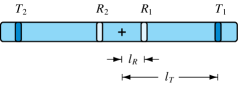
Figure 1: A schematic LWD instrument with two transmitters and two receivers symmetrically located around the tool center.

Triaxial logging instruments generate measurements for all possible orientations of the transmitter–receiver pairs. We follow the notation presented in [40, 25] to denote the magnetic field. Thus, we write ${\text{H}_{ZZ}^{T_{i}R_{j}}\in\mathbb{C}}$ as the coaxial magnetic field in the borehole system of coordinates induced by source $T_{i}$ and measured at receiver $R_{j}$ (${i,j=1,2}$). We use the magnetic fields measured at $R_{1}$ and $R_{2}$ to compute the attenuation ratio and phase difference. We symmetrize the signal originating from $T_{1}$ and $T_{2}$ to obtain the quantity of interest $\text{Q}_{ZZ}$ at each logging position as

$$\text{Q}_{ZZ}\coloneqq\dfrac{1}{2}\left(\log\dfrac{\text{H}_{ZZ}^{T_{1}R_{1}}}{\text{H}_{ZZ}^{T_{1}R_{2}}}+\log\dfrac{\text{H}_{ZZ}^{T_{2}R_{2}}}{\text{H}_{ZZ}^{T_{2}R_{1}}}\right)\,.$$ (18)

Then, we compute the attenuation ratio $(A)$ and phase difference $(P)$, respectively, as the real and imaginary parts of $\text{Q}_{ZZ}$:

$$A \coloneqq\text{Re}\!\>(\text{Q}_{ZZ})\,,$$ (19)

$$P \coloneqq\text{Im}\!\>(\text{Q}_{ZZ})\,.$$ (20)

We can then obtain the apparent resistivities based on the attenuation and phase ( ${\rho_{A}}$ and ${\rho_{P}}$, respectively) using a look-up algorithm presented in [41].

4 Refined isogeometric analysis

In this work, we consider a multi-field EM problem and discretize the 2.5D variational formulation of Eq. (15) using a B-spline generalization of a curl-conforming space, introduced by Buffa et al. [28]. We first review some basic concepts of high-continuity IGA discretizations.

4.1 High-continuity IGA discretization

Given the parametric domain ${\big{\{}\xi,\zeta\in\hat{\OM}_{x,z}:(0,1)^{2}\subset\mathbb{R}^{2}\big{\}}}$, we introduce the spline space ${\altmathcal{S}^{p_{x},p_{z}}_{k_{x},k_{z}}}$ as

$$\altmathcal{S}^{p_{x},p_{z}}_{k_{x},k_{z}}\coloneqq\text{span}\ack{B_{i,j}^{\!\>p_{x},p_{z}}}_{i=0,j=0}^{n_{x}-1,\!\>n_{z}-1}\,,$$ (21)

where $n$, $p$, and $k$ with their indices are the number of degrees of freedom, polynomial degree, and continuity of basis functions in $x$ and $z$ directions, respectively. The bivariate basis functions are

$$B_{i,j}^{\!\>p_{x},p_{z}}\coloneqq B_{i}^{\!\>p_{x}}(\xi)\otimes B_{j}^{\!\>p_{z}}(\zeta)\,,\qquad i=0,1,...,n_{x}-1\,,\quad j=0,1,...,n_{z}-1\,,$$ (22)

where the univariate bases are expressed by the Cox–De Boor recursion formula [42] as

$$B_{i}^{\!\>0}(\xi) =\left\{\begin{array}[]{ll}1&\xi_{i}\leq\xi<\xi_{i+1}\,,\\ 0&\mbox{otherwise}\,,\end{array}\right.$$ (23)

$$B_{i}^{\!\>p}(\xi) =\dfrac{\xi-\xi_{i}}{\xi_{i+p}-\xi_{i}}B_{i}^{\!\>{p-1}}(\xi)+\dfrac{\xi_{i+p+1}-\xi}{\xi_{i+p+1}-\xi_{i+1}}B_{{i+1}}^{\!\>{p-1}}(\xi)\,,$$

and spanned over the respective knot sequences in $x$ and $z$ directions, given by

$$\Xi =[\underbrace{0,0,...,0}_{p_{x}+1},\xi_{p_{x}+1},\xi_{p_{x}+2}...,\xi_{n_{x}-1},\underbrace{1,1,...,1}_{p_{x}+1}]\,,$$ (24)

Z $$=[\underbrace{0,0,...,0}_{p_{z}+1},\zeta_{p_{z}+1},\zeta_{p_{z}+2}...,\zeta_{n_{z}-1},\underbrace{1,1,...,1}_{p_{z}+1}]\,.$$ (25)

We assume single multiplicities for all knots, providing maximum continuity $k=p-1$ for the IGA discretization.

Fig. 2 illustrates the ${\textit{{H}}(\text{curl})\times H^{1}}$ IGA discrete space in $\OM_{x,z}$ along with the univariate basis functions of the respective vector fields. For brevity, herein and in the following, we exclude the superscript $\beta$ in referring to the components of the magnetic field.

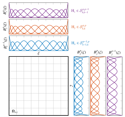
Figure 2: Example of the ${\textit{{H}}(\text{curl})\times H^{1}}$ space for a 2.5D formulation discretized by $C^{p-1}$ IGA with uniform ${8\times 8}$ elements in ${\OM_{x,z}}$, polynomial degree ${p=4}$, and continuity ${k=3}$. The univariate basis functions of $\text{H}_{x}$, $\text{H}_{y}$, and $\text{H}_{z}$ are shown in blue, red, and purple, respectively. Thin gray lines in the mesh skeleton denote the high-continuity element interfaces.

We define the spaces in the parametric domain and introduce the appropriate transformations to obtain the discretization on the physical domain. We start with the set of discrete spaces in the parametric domain, given by

$$\hat{\altmathcal{V}}_{h}^{\,\text{curl}}(\hat{\OM}_{x,z}) \coloneqq\altmathcal{S}^{p-1,p}_{k-1,k}\times\altmathcal{S}^{p,p-1}_{k,k-1}\,,$$ (26)

$$\hat{\altmathcal{Q}}_{h}^{\,\text{grad}}(\hat{\OM}_{x,z}) \coloneqq\altmathcal{S}^{p,p}_{k,k}\,.$$ (27)

By defining ${\textbf{F}:\hat{\OM}_{x,z}\rightarrow\OM_{x,z}}$ as the geometric mapping from the parametric domain onto the physical domain, and $D\textbf{F}$ as its Jacobian, we introduce the set of discrete spaces in the physical domain:

$$\altmathcal{V}_{h}^{\,\text{curl}}(\OM_{x,z}) \coloneqq\ack{\textbf{H}_{x,z}=\big{[}\text{H}_{x}\,,\text{H}_{z}\big{]}^{T}\in\textit{{H}}(\text{curl}^{\,\beta};\!\>\OM_{x,z})\cap\textit{{H}}^{1}(\OM_{x,z}):\iota^{\!\>\text{curl}}(\textbf{H}_{x,z})=\hat{\textbf{H}}_{x,z}\in\hat{\altmathcal{V}}_{h}^{\,\text{curl}}(\hat{\OM}_{x,z})}\,,$$ (28)

$$\altmathcal{Q}_{h}^{\,\text{grad}}(\OM_{x,z}) \coloneqq\ack{\text{H}_{y}\in H^{1}(\OM_{x,z}):\iota^{\!\>\text{grad}}(\text{H}_{y})=\hat{\text{H}}_{y}\in\hat{\altmathcal{Q}}_{h}^{\,\text{grad}}(\hat{\OM}_{x,z})}\,,$$ (29)

where we use the following curl- and grad-preserving pullback mappings [38, 28]:

$$\iota^{\!\>\text{curl}}(\textbf{H}_{x,z}) \coloneqq(D\textbf{F})^{T}(\textbf{H}_{x,z}\circ\textbf{F})\,,$$ (30)

$$\iota^{\!\>\text{grad}}(\text{H}_{y}) \coloneqq\text{H}_{y}\circ\textbf{F}\,.$$ (31)

Thus, by defining the discrete space

$$\altmathcal{H}_{h,0}(\OM_{x,z})\coloneqq\ack{\textbf{H}_{\beta,h}\in\altmathcal{V}_{h}^{\,\text{curl}}(\OM_{x,z})\times\altmathcal{Q}_{h}^{\,\text{grad}}(\OM_{x,z}):\textbf{H}_{\beta,h}\times\mathbf{n}=\mathbf{0}\text{ on }\partial{\OM}}\,,$$ (32)

we write the discrete form of Eq. (15) as follows (subscript $h$ refers to discrete solution):

$$\begin{cases}\begin{aligned} &\text{Find }\textbf{H}_{h}=\textstyle\rmsum_{\beta=-\infty}^{+\infty}\textbf{H}_{\beta,h}\,\text{exp}\!\>\big{(}\textrm{i\!\>}2\pi\beta y/L_{y}\big{)}\,,~{}\textbf{H}_{\beta,h}\in\altmathcal{H}_{h,0}(\OM_{x,z})\\[3.0pt] &\text{such that for every }\beta\in\mathbb{Z}{\rm~{}and~{}}\textbf{W}_{\beta,h}\in\altmathcal{H}_{h,0}(\OM_{x,z})\,,\\[2.0pt] &\qquad\left(\nabla^{\beta}\times\textbf{W}_{\beta,h}\,,\dfrac{1}{\sigma+\textrm{i\!\>}\omega\varepsilon}\nabla^{\beta}\times\textbf{H}_{\beta,h}\right)_{(L^{2}(\OM_{x,z}))^{3}}+\textrm{i\!\>}\omega\mu\left(\textbf{W}_{\beta,h},\textbf{H}_{\beta,h}\right)_{(L^{2}(\OM_{x,z}))^{3}}=-\textrm{i\!\>}\omega\mu\left(\textbf{W}_{\beta,h},\textbf{M}_{\beta}\right)_{(L^{2}(\OM_{x,z}))^{3}}\,.\end{aligned}\end{cases}$$ (33)

4.2 rIGA discretization

The refined isogeometric analysis (rIGA) is a discretization technique that optimizes the performance of direct solvers. In particular, rIGA preserves the optimal convergence order of the direct solvers with respect to a fixed number of elements in the domain. Garcia et al. [37] first presented this strategy for $H^{1}$ spaces and then extended it to $\textit{{H}}(\text{curl})$, $\textit{{H}}(\text{div})$, and $L^{2}$ spaces (see [38]). Starting from the high-continuity $C^{p-1}$ IGA discretization, rIGA reduces the continuity of certain basis functions by increasing the multiplicity of the respective existing knots. Hence, the computational domain is subdivided into high-continuity macroelements interconnected by low-continuity hyperplanes. These hyperplanes coincide with the locations of the separators at different partitioning levels of the multifrontal direct solvers. Thus, rIGA reduces the computational cost of matrix factorization when solving PDE systems in comparison to IGA and FEA.

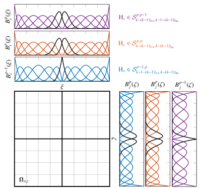
Figure 3: ${\textit{{H}}(\text{curl})\times H^{1}}$ rIGA space of the ${8\times 8}$ domain of Fig. 2 with ${p=4}$ and ${k=3}$, after one level of symmetric partitioning by the rIGA discretization that results in ${4\times 4}$ macroelements. rIGA reduces the continuity of basis functions by $k-1$ degrees across the macroelement separators (the low-continuity bases are shown in black). Thin gray lines in the mesh skeleton denote the high-continuity element interfaces, while thick black lines illustrate the macroelement boundaries. We refer to the vertical and horizontal separators as “vs” and “hs”, respectively.

For multi-field problems discretized using ${\textit{{H}}(\text{curl})\times H^{1}}$ spaces, we preserve the commutativity of the de Rham diagram [43] by reducing the continuity in ${k-1}$ degrees. To achieve this, we use both $C^{\!\>0}$ and $C^{1}$ hyperplanes and reduce the continuity across the interface between the subdomains (i.e., macroelements). Fig. 3 depicts the rIGA discretization of the ${\textit{{H}}(\text{curl})\times H^{1}}$ space of Fig. 2 after one level of symmetric partitioning, which results in macroelements containing ${4\times 4}$ elements.

Previous works show rIGA discretizations provide large improvements in the solution time and memory requirements. In particular, the rIGA solution is obtained up to $\altmathcal{O}(p^{2})$ faster in large domains —​ and $\altmathcal{O}(p)$ faster in small domains​ — than the IGA solution. In comparison to traditional FEA with the same number of elements, rIGA provides even larger improvements. rIGA also reduces the memory requirements since the rIGA LU factors have fewer nonzero entries than the IGA LU factors. Finally, rIGA improves the approximation error with respect to IGA since the continuity reduction of basis functions enriches the Galerkin space (see [37, 38]).

5 Implementation details

We implement discrete ${\textit{{H}}(\text{curl})\times H^{1}}$ spaces using PetIGA-MF [44], a multi-field extension of PetIGA [45], a high-performance isogeometric analysis implementation based on PETSc (portable extensible toolkit for scientific computation) [46]. PetIGA-MF allows the use of different spaces for each field of interest and employs data management libraries to condense the data of multiple fields in a single object, thus simplifying the discretization construction. This framework also allows us to investigate both IGA and rIGA discretizations in our 2.5D problem with different numbers of elements, different polynomial degrees of the B-spline spaces, and different partitioning levels of the mesh.

We use Intel MKL with PARDISO [47, 48] as our sparse direct solver package to construct LU factors for solving the linear systems of equations. PARDISO employs supernode techniques to perform the matrix factorization (see, e.g., [49, 50]). It provides parallel factorization using OpenMP directives [51] and uses the automatic matrix reordering provided by METIS [52]. We executed all tests on a workstation equipped with two Intel Xeon Gold 6230 CPUs at 2.10 GHz with 40 threads per CPU.

We employ a tensor-product mesh with variable element sizes (see Fig. 4). At each logging position, the computational mesh has a fine subgrid in the central part of the domain with element size equal to ${h\times h}$. This subgrid is surrounded by another tensor-product grid whose element sizes grow slowly until reaching the boundary.

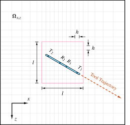
Figure 4: A drawing of the computational domain $\OM_{x,z}$ and the tool trajectory. The central subgrid bounded by a magenta box is composed of a set of fine elements located in the proximity of the logging instrument. The remaining elements grow smoothly in size until reaching the boundary.

Remark 1.

For each logging position, we perform a single symbolic factorization common to all Fourier modes, followed by a numerical factorization per Fourier mode. Once we solve the system of equations for the first transmitter, we update the right-hand side of Eq. (33) to solve for the magnetic field induced by the second transmitter and use backward substitution. Hence, we perform only one LU factorization per Fourier mode per logging position for both transmitters.

Remark 2.

The convergence of the Fourier series leads to a fast decay of the real and imaginary parts of $\text{H}_{ZZ}$ for higher Fourier modes (see [39]). Thus, we truncate the series of Eq. (10) when the magnetic field at the receivers is sufficiently small, such that ${\beta\in[-N_{f},N_{f}]}$, being $2N_{f}+1$ the total number of Fourier modes. In here, because of the symmetry of the media along the $y$ direction, we only consider ${\beta\in[0,N_{f}]}$.

6 Numerical Results

In this section, we first assess the accuracy of the rIGA approach in a homogeneous medium. We also investigate the computational efficiency of the rIGA framework in comparison with IGA and FEA approaches. Then, we consider two model problems consisting of high-angle wells crossing spatially heterogeneous media with multiple geological faults. Finally, we produce our synthetic training dataset for DL inversion. In our simulations, we consider one operational mode of a commercial logging tool [53] with ${l_{\!\>R}=10.16~{}\rm cm}$ and ${l_{\!\>T}=56.8325~{}\rm cm}$ (see Fig. 1). We select the free space electric permittivity and magnetic permeability, i.e., ${\varepsilon=8.85\times 10^{-12}~{}\rm F\cdot m^{-1}}$ and ${\mu=4\pi\times 10^{-7}~{}\rm N\cdot A^{-2}}$, respectively. We also consider a source frequency ${f=2~{}\rm MHz}$.

6.1 Homogeneous medium

We assume the logging instrument is placed in a homogeneous medium with electrical conductivity ${\sigma=0.01~{}(\Omega\cdot\rm m)^{-1}}$. This high-resistivity case is numerically more challenging than low-resistivity cases since it requires a larger number of Fourier modes and numerical precision.

6.1.1 Accuracy assessment

To assess the accuracy and select certain discretization parameters, we compare the numerical attenuation ratio, $A$, and phase difference, $P$, given by Eqs. (19) and (20), with the expected (i.e., exact) values, $A_{e}$ and $P_{e}$, obtained from ​ ${\rho_{e}=1/\sigma}$. Fig. 5 shows the numerical errors, i.e., ${\left\lvert 1-A/A_{e}\right\rvert}$ and ${\left\lvert 1-P/P_{e}\right\rvert}$, as a function of the number of Fourier modes when computing attenuation and phase in the homogeneous medium. Herein, we select a domain with ${64\times 64}$ elements to ensure a fast numerical solution for our measurements. We compare the high-continuity ${C^{p-1}}$ IGA with an rIGA discretization that employs ${8\times 8}$ macroelements. This macroelement size provides the fastest results for moderate size domains (see [37]). We consider three different mesh sizes —​ ${h=0.025~{}{\rm m},~{}0.33~{}{\rm m},~{}{\rm and}~{}0.50~{}{\rm m}}$​ — and different polynomial degrees —​ ${p=3,~{}4,{~{}\rm and}~{}5}$. The best results correspond to $h=0.025~{}{\rm m}$ (blue lines in the figure). We also observe that rIGA discretizations (dashed and dotted lines) deliver lower errors compared to their IGA counterparts.

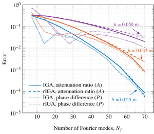
(a) $p=3$

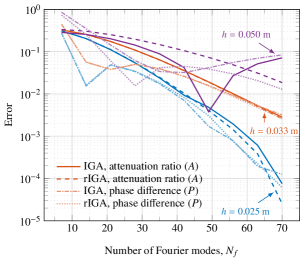
(b) $p=4$

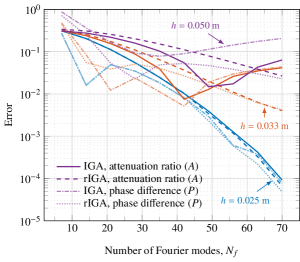
(c) $p=5$

Figure 5: Numerical errors when computing attenuation ratio, $A$, and phase difference, $P$, in a homogeneous medium using IGA and rIGA discretizations, obtained by for a ${64\times 64}$ mesh with different element sizes $h$ and polynomial degrees $p$.

To investigate the decay of the solution for each Fourier mode, we compare numerical results with the analytical 2.5D solution in the homogeneous medium presented in [25]. In particular, given $M_{z}$ as the only nonzero component of the magnetic source, it is possible to analytically determine the coaxial magnetic field for each Fourier mode as

$$\text{H}_{ZZ}(\,\beta\!\>)=-\textrm{i\!\>}\omega\mu\sigma\tau_{\beta_{z}}+\dfrac{\partial^{\!\>2}\tau_{\beta_{z}}}{\partial z^{2}}\,,$$ (34)

with

$$\tau_{\beta_{z}}=\dfrac{M_{z}}{2\pi}\dfrac{1}{L_{y}}K_{0}({\rm C}R)\,\text{exp}\!\>\big{(}\textrm{i\!\>}2\pi\beta y_{0}/L_{y}\big{)}\,,$$ (35)

where $K_{0}(\cdot)$ is the modified Bessel function of the second kind of order zero, and

$${\rm C} =\left(2\pi\beta/L_{y}\right)^{2}+\textrm{i\!\>}\omega\mu\sigma\,,$$ (36)

$$R =\sqrt{(x-x_{0})^{2}+(z-z_{0})^{2}}\,.$$ (37)

Fig. 6 compares the decay of the numerical coaxial magnetic field ${\text{H}_{ZZ}(\,\beta\!\>)}$ with its analytical counterpart for some Fourier modes. Using a domain with ${64\times 64}$ elements and ${h=0.025~{}{\rm m}}$, we monitor the decay of the propagated waves at distances within the interval ${[0.2,1.0]~{}{\rm m}}$ from the transmitters to ensure that the solutions at both receivers properly approximate the analytical ones. Results show that rIGA discretizations deliver increased accuracy for all tested polynomial degrees.

(a) $p=3$

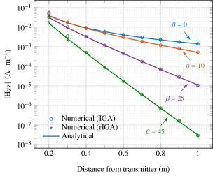
(b) $p=4$

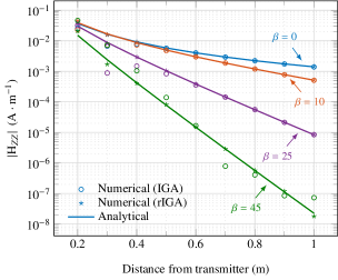
(c) $p=5$

Figure 6: Comparison of the decay of the numerical and analytical coaxial magnetic fields for some Fourier modes, obtained in a grid of ${64\times 64}$ elements with ${h=0.025~{}{\rm m}}$ and different polynomial degrees.

6.1.2 Computational efficiency

Works [37, 38] provide theoretical cost estimates of solving $H^{1}$ and $\textit{{H}}(\text{curl})$ discrete spaces, respectively. Herein, we add these estimates to predict the cost of discretizing the ${\textit{{H}}(\text{curl})\times H^{1}}$ space appearing in our 2.5D EM problem. We conclude that the cost of LU factorization of the rIGA matrix for this combined space is between ${\altmathcal{O}(p)}$ and ${\altmathcal{O}(p^{2})}$ times smaller than that for IGA. Details are omitted for the sake of simplicity.

To numerically assess the computational efficiency confirming the aforementioned theoretical results, we consider two different grids in $\OM_{x,z}$ with ${64\times 64}$ and ${128\times 128}$ elements, respectively. Using continuity reduction, we split the mesh symmetrically into macroelements whose sizes are powers of two. In this context, the maximum-continuity $C^{p-1}$ IGA discretization is composed of one macroelement containing the entire grid, while FEA with $C^{\!\>0}$ continuity across all element interfaces is composed of macroelements that contain only one element. Fig. 7 shows the number of FLOPs and time required to solve the borehole resistivity problem for each Fourier mode per logging position. We compare the computational costs for different polynomial degrees and different continuity reduction levels of basis functions. The cost of rIGA reaches the minimum with ${8\times 8}$ macroelements almost in all cases, confirming the theoretical estimates obtained from the results of [37].

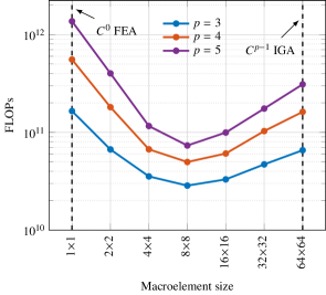
(a) FLOPs ($64\times 64$ elements)

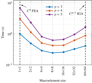
(b) Time ($64\times 64$ elements)

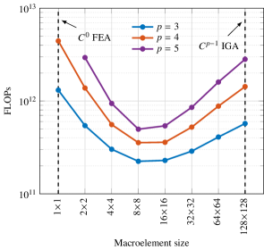
(c) FLOPs ($128\times 128$ elements)

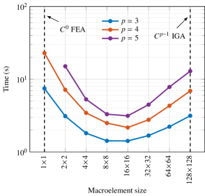
(d) Time ($128\times 128$ elements)

Figure 7: Computational cost in terms of FLOPs and time for solving a 2.5D borehole resistivity problem per logging position per Fourier mode. We test rIGA discretizations with two different grids of ${64\times 64}$ and ${128\times 128}$ elements. The computational times correspond to the use of parallel solver PARDISO using two threads.

Our numerical tests show that for a moderate size 2.5D problem, the reduction in the number of FLOPs is $\altmathcal{O}(p)$ with respect to IGA. When compared to FEA, rIGA delivers larger improvement factors. These improvement factors in terms of FLOPs also hold in terms of time when performing a sequential factorization. In our parallel PARDISO solver, we observe a small degradation of the rIGA improvement factors in terms of times in comparison to those obtained in terms of FLOPs (see Table 1).

Table 1: Computational cost for the 2.5D borehole resistivity measurements per logging position per Fourier mode. We report the solution time and FLOPs when using $C^{p-1}$ IGA, rIGA with ${8\times 8}$ macroelements, and $C^{\!\>0}$ FEA with the same number of elements and polynomial degree. The computational times correspond to the use of parallel solver PARDISO using two threads.

Domain size	Polynomial degree	Discretization method	Number of FLOPs	Improvement factor (FLOPs)		Time (s)	Improvement factor (time)
64​ $\times$​ 64	3	IGA	6.56e+10			0.407
		rIGA	2.85e+10	IGA/rIGA	2.30	0.242	IGA/rIGA	1.68
		FEA	1.65e+11	FEA/rIGA	5.79	0.999	FEA/rIGA	4.12
	4	IGA	1.62e+11			0.875
		rIGA	4.97e+10	IGA/rIGA	3.26	0.419	IGA/rIGA	2.09
		FEA	5.56e+11	FEA/rIGA	11.19	3.061	FEA/rIGA	7.29
	5	IGA	3.10e+11			1.645
		rGA	7.33e+10	IGA/rIGA	4.23	0.620	IGA/rIGA	2.65
		FEA	1.37e+12	FEA/rIGA	18.69	6.806	FEA/rIGA	10.98
128​ $\times$​ 128	3	IGA	5.72e+11			3.144
		rIGA	2.24e+11	IGA/rIGA	2.55	1.423	IGA/rIGA	2.21
		FEA	1.31e+12	FEA/rIGA	5.85	7.456	FEA/rIGA	5.24
	4	IGA	1.43e+12			6.903
		rIGA	3.56e+11	IGA/rIGA	4.02	2.495	IGA/rIGA	2.77
		FEA	4.44e+12	FEA/rIGA	12.47	22.885	FEA/rIGA	9.17
	5	IGA	2.82e+12			12.911
		rGA	4.97e+11	IGA/rIGA	5.67	3.305	IGA/rIGA	3.91
		FEA	–	FEA/rIGA	–	–	FEA/rIGA	–

6.2 Heterogeneous media

We further examine the accuracy of our rIGA approximation over two synthetic heterogeneous model problems.

6.2.1 One geological fault

We consider the model problem of Fig. 8 with a constant dip angle of $80^{\circ}$. We consider the LWD instrument described in Section 3 and simulate measurements recorded over 200 equally-spaced logging positions throughout the well trajectory.

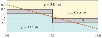
Figure 8: Model problem with a constant-angle well trajectory (red dashed line) passing through a geological fault and three different materials. Dimensions are in meters.

Fig. 9 shows the apparent resistivities based on the attenuation and phase ( $\rho_{A}$ and $\rho_{P}$, respectively). We obtain the results using ${N_{f}=70}$ and an rIGA discretization with ${64\times 64}$ elements, ${p=4}$, and ${8\times 8}$ macroelements. Results are in good agreement with those presented in [25].

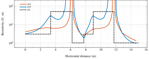
Figure 9: Apparent resistivities based on the attenuation, $\rho_{A}$, and phase, $\rho_{P}$, for the first model problem, compared with the real resistivity, $\rho_{e}$. We obtain the results using an rIGA discretization with ${64\times 64}$ elements, ${p=4}$, and ${8\times 8}$ macroelements.

6.2.2 Two geological faults and inclined layers

Fig. 10 shows the second model problem containing two geological faults and inclined layers. The logging trajectory starts from a sandstone layer with a resistivity of ${\rho=3~{}\Omega\cdot\rm m}$, and passes through an oil-saturated layer with ${\rho=100~{}\Omega\cdot\rm m}$. The tool trajectory also passes through a water-saturated layer with ${\rho=0.5~{}\Omega\cdot\rm m}$.

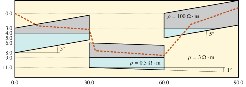
Figure 10: Second model problem with two geological faults and inclined layers. The tool trajectory (red dashed line) has different dip angles and passes through sandstone (yellow), oil-saturated (gray) and water-saturated (green) layers. Dimensions are in meters.

In particular, inclined layers produce the so-called staircase approximations [54]. This phenomenon occurs because the physical interfaces of the conductivity model are not aligned with the element edges. Thus, the conductivity parameter takes different values inside some elements of the mesh. To tackle this issue, discretization techniques using nonfitting grids [26, 55] are available, but they have not been considered here for simplicity.

Fig. 11 shows the apparent resistivities based on the attenuation and phase throughout the logging trajectory and compares their value with the exact resistivity. We simulate the resistivities at 1,080 logging positions with ${N_{f}=70}$. We use an rIGA discretization with ${64\times 64}$ elements, ${p=4}$, and ${8\times 8}$ macroelements.

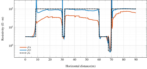
Figure 11: Apparent resistivities based on the attenuation, $\rho_{A}$, and phase, $\rho_{P}$, for the second model problem, compared with the real resistivity, $\rho_{e}$. We obtain the results using an rIGA discretization with ${64\times 64}$ elements, ${p=4}$, and ${8\times 8}$ macroelements.

6.3 Database generation for DL inversion

To produce our synthetic training dataset for DL inversion, we consider heterogeneous medium containing three different layers and six varying parameters at each logging position, as described in Fig. 12 and Table 2. We select three different electrical conductivities: $\sigma_{c}$ for the central layer, and $\sigma_{u}$ and $\sigma_{l}$ for the upper and lower layers, respectively. We assume the tool center is always within the middle layer and has vertical distances of $d_{u}$ and $d_{l}$ from the upper and lower layers, respectively. The sixth varying parameter is the dip angle, $\varphi$​ , measured from the vertical direction.

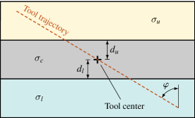
Figure 12: Varying parameters at each logging position when producing the training dataset for DL inversion.

In here, we create a dataset of 100,000 samples and compute the apparent resistivities obtained from random combinations within a given range of resistivities ${\rho=1/\sigma\in[1,100]~{}\Omega\cdot\rm m}$ (see Table 2).

Table 2: Varying parameters employed to generate the training dataset for DL inversion.

Varying parameters		Interval
Electrical conductivity of the central layer	$\log_{10}(\sigma_{c}$)	$[-2,0]$
Electrical conductivity of the upper layer	$\log_{10}(\sigma_{u}$)	$[-2,0]$
Electrical conductivity of the lower layer	$\log_{10}(\sigma_{l}$)	$[-2,0]$
Distance of the tool center from the upper layer	$\log_{10}(d_{u}$)	$[-2,1]$
Distance of the tool center from the lower layer	$\log_{10}(d_{l}$)	$[-2,1]$
Dip angle between the tool and the layered media	$\varphi$	$[80^{\circ},100^{\circ}]$

For generating the dataset, we use two different types of parallelization. One parallelization is related to the parallel factorization of the direct solver, and the other is the trivial parallelization based on scheduling the solutions of independent earth models onto different processors. Using 40 threads, we solve for 20 different earth models, each executing over two threads. Table 1 shows that the required time for matrix factorization of the 2.5D EM problem using optimal rIGA discretization with ${64\times 64}$ grid, ${p=4}$, and ${8\times 8}$ macroelements is about 0.42 seconds per Fourier mode. Considering ${N_{f}=70}$, and the additional time required for pre/postprocessing and inter-thread communications, each set of independent runs (consists of 20 different earth models) takes about 40 seconds. Thus, we perform 5,000 sequential runs to construct our 100,000 samples in about 56 hours. To create a larger database, we could execute over a cluster of hundreds of CPUs/threads, expecting a perfect parallel scalability.

Fig. 13(a) depicts the graphs of attenuation ratio, $A$, versus phase difference, $P$, obtained from the 100,000 earth models when using rIGA discretization for generating the database. Since there is a strong correlation between $A$ and $P$, the data distribution on the plot follows an almost straight line. We also display in Fig. 13(b) the correlation between apparent resistivities based on attenuation and phase.

\begin{overpic}[width=433.62pt,trim=0.0pt 0.0pt 56.9055pt 0.0pt,clip]{Figs/AttPhs} \put(42.0,0.0){\footnotesize Phase difference, $P$} \put(11.0,5.0){\footnotesize$-0.2$} \put(21.25,5.0){\footnotesize$-0.1$} \put(32.5,5.0){\footnotesize$0.0$} \put(42.75,5.0){\footnotesize$0.1$} \put(53.0,5.0){\footnotesize$0.2$} \put(63.25,5.0){\footnotesize$0.3$} \put(73.5,5.0){\footnotesize$0.4$} \put(83.75,5.0){\footnotesize$0.5$} \put(94.0,5.0){\footnotesize$0.6$} \put(6.5,8.0){\footnotesize$0.95$} \put(6.5,14.75){\footnotesize$1.00$} \put(6.5,21.5){\footnotesize$1.05$} \put(6.5,28.25){\footnotesize$1.10$} \put(6.5,35.0){\footnotesize$1.15$} \put(6.5,41.75){\footnotesize$1.20$} \put(6.5,48.5){\footnotesize$1.25$} \put(6.5,55.25){\footnotesize$1.30$} \put(6.5,62.0){\footnotesize$1.35$} \put(6.5,68.75){\footnotesize$1.40$} \put(6.5,75.5){\footnotesize$1.45$} \begin{turn}{90.0} \put(29.0,0.0){\footnotesize Attenuation ratio, $A$} \end{turn} \end{overpic}

(a)

\begin{overpic}[width=433.62pt,trim=0.0pt 0.0pt 56.9055pt 0.0pt,clip]{Figs/AppRes} \put(34.0,0.0){\footnotesize Apparent resistivity (phase), $\rho_{P}$} \put(15.0,5.0){\footnotesize$10^{\!\>0}$} \put(46.25,5.0){\footnotesize$10^{\!\>1}$} \put(77.5,5.0){\footnotesize$10^{\!\>2}$} \put(7.0,11.0){\footnotesize$10^{\!\>0}$} \put(7.0,36.5){\footnotesize$10^{\!\>1}$} \put(7.0,62.0){\footnotesize$10^{\!\>2}$} \begin{turn}{90.0} \put(17.0,0.0){\footnotesize Apparent resistivity (attenuation), $\rho_{A}$} \end{turn} \end{overpic}

(b)

Figure 13: (a) Attenuation ratio vs. phase difference, and (b) apparent resistivity based on attenuation vs. apparent resistivity based on phase, obtained for the 100,000 earth models. We use rIGA discretization with ${64\times 64}$ elements, ${p=4}$, and ${8\times 8}$ macroelements for generating the database.

7 Conclusions

We propose the use of refined isogeometric analysis (rIGA) discretizations for generating a (large) synthetic database for deep learning inversion of 2.5D borehole electromagnetic measurements. Such a database is essential for layer-by-layer estimation of the inverted earth models, which may be used for real-time adjustments of the well trajectory during geosteering operations.

rIGA delivers computational savings of up to $\altmathcal{O}(p)$ compared to the high-continuity isogeometric analysis (IGA). When compared to a traditional finite element analysis (FEA) with the same mesh size and polynomial degree, rIGA provides higher improvement factors. At the same time, rIGA provides sufficiently accurate solutions for geosteering purposes.

To create a dataset for deep learning inversion, we first selected certain discretization parameters based on the results of several homogeneous solutions. Then, we checked the accuracy over homogeneous and heterogeneous media. Finally, we generated a meaningful synthetic database composed of 100,000 earth models with the corresponding measurements in about 56 hours using a workstation equipped with two CPUs.

As future work, we propose the use of artificial intelligence based techniques to perform the inversion of a large set of borehole resistivity measurements with earth models containing multiple geological faults. To create a larger database, we propose to execute the presented method over a cluster of hundreds of CPUs/threads. We will also employ more complex earth model parameterizations including anisotropic layers.

References

References

- [1] C. R. Liu, Theory of Electromagnetic Well Logging, Elsevier, Amsterdam, Netherlands, 2017.
- [2] H. Liu, Principles and Applications of Well Logging, Springer, Berlin Heidelberg, Germany, 2017.
- [3] C. R. Vogel, Computational Methods for Inverse Problems, Society for Industrial and Applied Mathematics, Philadelphia, PA, 2002.
- [4] A. Tarantola, Inverse Problem Theory and Methods for Model Parameter Estimation, Society for Industrial and Applied Mathematics, Philadelphia, PA, 2005.
- [5] D. Watzenig, Bayesian inference for inverse problems – statistical inversion, e & i Elektrotechnik und Informationstechnik 124 (7-8) (2007) 240–247. doi:10.1007/s00502-007-0449-0.
- [6] J. Kaipio, E. Somersalo, Statistical inverse problems: Discretization, model reduction and inverse crimes, Journal of Computational and Applied Mathematics 198 (2) (2007) 493–504. doi:10.1016/j.cam.2005.09.027.
- [7] Q. Shen, J. Chen, X. Wu, Z. Han, Y. Huang, Parallel tempered trans-dimensional Bayesian inference for the inversion of ultra-deep directional logging-while-drilling resistivity measurements, Journal of Petroleum Science and Engineering 188 (2020) 106961. doi:10.1016/j.petrol.2020.106961.
- [8] Y. Kim, N. Nakata, Geophysical inversion versus machine learning in inverse problems, The Leading Edge 37 (12) (2018) 894–901. doi:10.1190/tle37120894.1.
- [9] F. Yang, J. Ma, Deep-learning inversion: A next-generation seismic velocity model building method, Geophysics 84 (4) (2019) R583–R599. doi:10.1190/geo2018-0249.1.
- [10] H. Li, H. Wang, L. Wang, X. Zhou, A modified Boltzmann annealing differential evolution algorithm for inversion of directional resistivity logging-while-drilling measurements, Journal of Petroleum Science and Engineering 188 (2020) 106916. doi:10.1016/j.petrol.2020.106916.
- [11] M. Shahriari, D. Pardo, A. Picon, A. Galdran, J. Del Ser, C. Torres-Verdín, A deep learning approach to the inversion of borehole resistivity measurements, Computational Geosciences 24 (3) (2020) 971–994. doi:10.1007/s10596-019-09859-y.
- [12] M. Shahriari, D. Pardo, B. Moser, F. Sobieczky, A deep neural network as surrogate model for forward simulation of borehole resistivity measurements, Procedia Manufacturing 42 (2020) 235–238. doi:10.1016/j.promfg.2020.02.075.
- [13] A. Abubakar, T. Habashy, V. Druskin, D. Alumbaugh, A. Zerelli, L. Knizhnerman, Two-and-half-dimensional forward and inverse modeling for marine CSEM problems, in: SEG Technical Program Expanded Abstracts, Society of Exploration Geophysicists, 2006. doi:10.1190/1.2370366.
- [14] D. Pardo, C. Torres-Verdín, M. J. Nam, M. Paszynski, V. M. Calo, Fourier series expansion in a non-orthogonal system of coordinates for the simulation of 3D alternating current borehole resistivity measurements, Computer Methods in Applied Mechanics and Engineering 197 (45-48) (2008) 3836–3849. doi:10.1016/j.cma.2008.03.007.
- [15] J. Shen, W. Sun, 2.5-D modeling of cross-hole electromagnetic measurement by finite element method, Petroleum Science 5 (2) (2008) 126–134. doi:10.1007/s12182-008-0020-6.
- [16] M. J. Nam, D. Pardo, C. Torres-Verdín, Simulation of borehole-eccentered triaxial induction measurements using a Fourier finite-element method, Geophysics 78 (1) (2013) D41–D52. doi:10.1190/geo2011-0524.1.
- [17] S. Gernez, A. Bouchedda, E. Gloaguen, D. Paradis, Aim4res, an open-source 2.5D finite differences MATLAB library for anisotropic electrical resistivity modeling, Computers & Geosciences 135 (2020) 104401. doi:10.1016/j.cageo.2019.104401.
- [18] D. Pardo, C. Torres-Verdín, Fast 1D inversion of logging-while-drilling resistivity measurements for improved estimation of formation resistivity in high-angle and horizontal wells, Geophysics 80 (2) (2015) E111–E124. doi:10.1190/geo2014-0211.1.
- [19] S. A. Bakr, D. Pardo, C. Torres-Verdín, Fast inversion of logging-while-drilling resistivity measurements acquired in multiple wells, Geophysics 82 (3) (2017) E111–E120. doi:10.1190/geo2016-0292.1.
- [20] M. Shahriari, D. Pardo, Borehole resistivity simulations of oil-water transition zones with a 1.5D numerical solver, Computational Geosciences 24 (3) (2020) 1285–1299. doi:10.1007/s10596-020-09946-5.
- [21] D. Pardo, L. Demkowicz, C. Torres-Verdín, M. Paszynski, Two-dimensional high-accuracy simulation of resistivity logging-while-drilling (LWD) measurements using a self-adaptive goal-oriented finite element method, SIAM Journal on Applied Mathematics 66 (6) (2006) 2085–2106. doi:10.1137/050631732.
- [22] V. M. Calo, D. Pardo, M. R. Paszyński, Goal-oriented self-adaptive finite element simulation of 3D DC borehole resistivity simulations, Procedia Computer Science 4 (2011) 1485–1495. doi:10.1016/j.procs.2011.04.161.
- [23] Z. Ma, D. Liu, H. Li, X. Gao, Numerical simulation of a multi-frequency resistivity logging-while-drilling tool using a highly accurate and adaptive higher-order finite element method, Advances in Applied Mathematics and Mechanics 4 (4) (2012) 439–453. doi:10.1017/S2070073300001739.
- [24] H. Wang, G. Tao, K. Zhang, Wavefield simulation and analysis with the finite-element method for acoustic logging while drilling in horizontal and deviated wells, Geophysics 78 (6) (2013) D525–D543. doi:10.1190/geo2012-0542.1.
- [25] Á. Rodríguez-Rozas, D. Pardo, C. Torres-Verdín, Fast 2.5D finite element simulations of borehole resistivity measurements, Computational Geosciences 22 (5) (2018) 1271–1281. doi:10.1007/s10596-018-9751-7.
- [26] T. Chaumont-Frelet, D. Pardo, Á. Rodríguez-Rozas, Finite element simulations of logging-while-drilling and extra-deep azimuthal resistivity measurements using non-fitting grids, Computational Geosciences 22 (5) (2018) 1161–1174. doi:10.1007/s10596-018-9744-6.
- [27] T. J. R. Hughes, J. A. Cottrell, Y. Bazilevs, Isogeometric analysis: CAD, finite elements, NURBS, exact geometry and mesh refinement, Computer Methods in Applied Mechanics and Engineering 194 (39-41) (2005) 4135–4195. doi:10.1016/j.cma.2004.10.008.
- [28] A. Buffa, G. Sangalli, R. Vázquez, Isogeometric analysis in electromagnetics: B-splines approximation, Computer Methods in Applied Mechanics and Engineering 199 (17-20) (2010) 1143–1152. doi:10.1016/j.cma.2009.12.002.
- [29] D. M. Nguyen, A. Evgrafov, J. Gravesen, Isogeometric shape optimization for electromagnetic scattering problems, Progress In Electromagnetics Research B 45 (2012) 117–146. doi:10.2528/pierb12091308.
- [30] A. Buffa, G. Sangalli, R. Vázquez, Isogeometric methods for computational electromagnetics: B-spline and T-spline discretizations, Journal of Computational Physics 257 (2014) 1291–1320. doi:10.1016/j.jcp.2013.08.015.
- [31] R. N. Simpson, Z. Liu, R. Vázquez, J. A. Evans, An isogeometric boundary element method for electromagnetic scattering with compatible B-spline discretizations, Journal of Computational Physics 362 (2018) 264–289. doi:10.1016/j.jcp.2018.01.025.
- [32] A. Simona, L. Bonaventura, C. de Falco, S. Schöps, IsoGeometric approximations for electromagnetic problems in axisymmetric domains, Computer Methods in Applied Mechanics and Engineering 369 (2020) 113211. doi:10.1016/j.cma.2020.113211.
- [33] S. Shahrokhabadi, T. D. Cao, F. Vahedifard, Isogeometric analysis through Bézier extraction for thermo-hydro-mechanical modeling of saturated porous media, Computers and Geotechnics 107 (2019) 176–188. doi:10.1016/j.compgeo.2018.11.012.
- [34] T. Hageman, K. M. P. Fathima, R. de Borst, Isogeometric analysis of fracture propagation in saturated porous media due to a pressurised non-Newtonian fluid, Computers and Geotechnics 112 (2019) 272–283. doi:10.1016/j.compgeo.2019.04.030.
- [35] J. A. Cottrell, T. J. R. Hughes, Y. Bazilevs, Isogeometric Analysis: Toward Integration of CAD and FEA, John Wiley & Sons, Ltd, New York, NY, 2009.
- [36] N. Collier, D. Pardo, L. Dalcin, M. Paszynski, V. M. Calo, The cost of continuity: A study of the performance of isogeometric finite elements using direct solvers, Computer Methods in Applied Mechanics and Engineering 213-216 (2012) 353–361. doi:10.1016/j.cma.2011.11.002.
- [37] D. Garcia, D. Pardo, L. Dalcin, M. Paszyński, N. Collier, V. M. Calo, The value of continuity: Refined isogeometric analysis and fast direct solvers, Computer Methods in Applied Mechanics and Engineering 316 (2017) 586–605. doi:10.1016/j.cma.2016.08.017.
- [38] D. Garcia, D. Pardo, V. M. Calo, Refined isogeometric analysis for fluid mechanics and electromagnetics, Computer Methods in Applied Mechanics and Engineering 356 (2019) 598–628. doi:10.1016/j.cma.2019.06.011.
- [39] Á. Rodríguez-Rozas, D. Pardo, A priori Fourier analysis for 2.5D finite elements simulations of logging-while-drilling (LWD) resistivity measurements, Procedia Computer Science 80 (2016) 782–791. doi:10.1016/j.procs.2016.05.368.
- [40] S. Davydycheva, Two triaxial induction tools: sensitivity to radial invasion profile, Geophysical Prospecting 59 (2) (2011) 323–340. doi:10.1111/j.1365-2478.2010.00910.x.
- [41] B. I. Anderson, Modeling and Inversion Methods for the Interpretation of Resistivity Logging Tool Response, DUP Science, Delft, Netherlands, 2001.
- [42] L. Piegl, W. Tiller, The NURBS Book, 2nd Edition, Springer-Verlag, New York, NY, 1997.
- [43] L. Demkowicz, P. Monk, L. Vardapetyan, W. Rachowicz, De Rham diagram for finite element spaces, Computers & Mathematics with Applications 39 (7-8) (2000) 29–38. doi:10.1016/s0898-1221(00)00062-6.
- [44] A. Sarmiento, A. Côrtes, D. Garcia, L. Dalcin, N. Collier, V. Calo, PetIGA-MF: A multi-field high-performance toolbox for structure-preserving B-splines spaces, Journal of Computational Science 18 (2017) 117–131. doi:10.1016/j.jocs.2016.09.010.
- [45] L. Dalcin, N. Collier, P. Vignal, A. M. A. Côrtes, V. M. Calo, PetIGA: A framework for high-performance isogeometric analysis, Computer Methods in Applied Mechanics and Engineering 308 (2016) 151–181. doi:10.1016/j.cma.2016.05.011.
- [46] S. Balay, W. D. Gropp, L. C. McInnes, B. F. Smith, Efficient management of parallelism in object oriented numerical software libraries, in: E. Arge, A. M. Bruaset, H. P. Langtangen (Eds.), Modern Software Tools in Scientific Computing, Birkhäuser Press, 1997, pp. 163–202.
- [47] C. G. Petra, O. Schenk, M. Anitescu, Real-time stochastic optimization of complex energy systems on high-performance computers, Computing in Science & Engineering 16 (5) (2014) 32–42. doi:10.1109/mcse.2014.53.
- [48] C. G. Petra, O. Schenk, M. Lubin, K. Gäertner, An augmented incomplete factorization approach for computing the Schur complement in stochastic optimization, SIAM Journal on Scientific Computing 36 (2) (2014) C139–C162. doi:10.1137/130908737.
- [49] O. Schenk, K. Gärtner, W. Fichtner, Efficient sparse LU factorization with left-right looking strategy on shared memory multiprocessors, BIT Numerical Mathematics 40 (1) (2000) 158–176. doi:10.1023/a:1022326604210.
- [50] O. Schenk, K. Gärtner, Solving unsymmetric sparse systems of linear equations with PARDISO, Future Generation Computer Systems 20 (3) (2004) 475–487. doi:10.1016/j.future.2003.07.011.
- [51] L. Dagum, R. Menon, OpenMP: an industry standard API for shared-memory programming, IEEE Computational Science and Engineering 5 (1) (1998) 46–55. doi:10.1109/99.660313.
- [52] G. Karypis, V. Kumar, A fast and high quality multilevel scheme for partitioning irregular graphs, SIAM Journal on Scientific Computing 20 (1) (1998) 359–392. doi:10.1137/s1064827595287997.
- [53] J. Zhou, LWD/MWD Resistivity Tool Parameters, Maxwell Dynamics, Houston, TX, 2016.
- [54] A. C. Cangellaris, D. B. Wright, Analysis of the numerical error caused by the stair-stepped approximation of a conducting boundary in FDTD simulations of electromagnetic phenomena, IEEE Transactions on Antennas and Propagation 39 (10) (1991) 1518–1525. doi:10.1109/8.97384.
- [55] T. Chaumont-Frelet, S. Nicaise, D. Pardo, Finite element approximation of electromagnetic fields using nonfitting meshes for geophysics, SIAM Journal on Numerical Analysis 56 (4) (2018) 2288–2321. doi:10.1137/16m1105566.