Reward Maximisation through Discrete Active Inference

Abstract

Active inference is a probabilistic framework for modelling the behaviour of biological and artificial agents, which derives from the principle of minimising free energy. In recent years, this framework has successfully been applied to a variety of situations where the goal was to maximise reward, offering comparable and sometimes superior performance to alternative approaches. In this paper, we clarify the connection between reward maximisation and active inference by demonstrating how and when active inference agents perform actions that are optimal for maximising reward. Precisely, we show the conditions under which active inference produces the optimal solution to the Bellman equation—a formulation that underlies several approaches to model-based reinforcement learning and control. On partially observed Markov decision processes, the standard active inference scheme can produce Bellman optimal actions for planning horizons of 1, but not beyond. In contrast, a recently developed recursive active inference scheme (sophisticated inference) can produce Bellman optimal actions on any finite temporal horizon. We append the analysis with a discussion of the broader relationship between active inference and reinforcement learning.

Keywords: Generative model; control as inference; dynamic programming; Bellman optimality; model-based reinforcement learning; discrete-time stochastic optimal control; Bayesian inference; Markov decision process

1 Introduction

1.1 Active inference

Active inference is a normative framework for modelling intelligent behaviour in biological and artificial agents. It simulates behaviour by numerically integrating equations of motion thought to describe the behaviour of biological systems, a description based on the free energy principle (Friston et al., 2022; Barp et al., 2022; Friston, 2010; Ramstead et al., 2022). Active inference comprises a collection of algorithms for modelling perception, learning, and decision-making in the context of both continuous and discrete state spaces (Friston et al., 2017c, 2021; Da Costa et al., 2020; Buckley et al., 2017; Barp et al., 2022; Friston et al., 2010). Briefly, building active inference agents entails: $1)$ equipping the agent with a (generative) model of the environment, $2)$ fitting the model to observations through approximate Bayesian inference by minimising variational free energy (i.e., optimising an evidence lower bound (Beal, 2003; Bishop, 2006; Jordan et al., 1998; Blei et al., 2017)) and $3)$ selecting actions that minimise expected free energy, a quantity that that can be decomposed into risk (i.e., the divergence between predicted and preferred paths) and ambiguity, leading to context-specific combinations of exploratory and exploitative behaviour (Schwartenbeck et al., 2019; Millidge, 2021). This framework has been used to simulate and explain intelligent behaviour in neuroscience (Parr et al., 2021; Adams et al., 2013; Parr, 2019; Sajid et al., 2022), psychology and psychiatry (Smith et al., 2022b, 2021a, 2021b, 2021c, 2020d, 2020a, 2021d, 2020b), machine learning (Millidge, 2020; Tschantz et al., 2020a, 2019; Fountas et al., 2020; Çatal et al., 2020; Mazzaglia et al., 2021) and robotics (Çatal et al., 2021; Lanillos et al., 2020; Sancaktar et al., 2020; Pio-Lopez et al., 2016; Pezzato et al., 2020; Oliver et al., 2021; Schneider et al., 2022).

1.2 Reward maximisation through active inference?

In contrast, the traditional approaches towards simulating and explaining intelligent behaviour—stochastic optimal control (Bertsekas and Shreve, 1996; Bellman, 1957) and reinforcement learning (RL; Barto and Sutton (1992))—derive from the normative principle of executing actions to maximise reward scoring the utility afforded by each state of the world. This idea dates back to expected utility theory (Von Neumann and Morgenstern, 1944), an economic model of rational choice behaviour, which also underwrites game theory (Von Neumann and Morgenstern, 1944) and decision theory (Dayan and Daw, 2008; Berger, 1985). Several empirical studies have shown that active inference can successfully perform tasks that involve collecting reward, often (but not always) showing comparative or superior performance to RL (Millidge, 2020; Paul et al., 2021; Cullen et al., 2018; van der Himst and Lanillos, 2020; Sajid et al., 2021a; Marković et al., 2021; Mazzaglia et al., 2021; Smith et al., 2022b, 2021b, 2021c, 2020d), and marked improvements when interacting with volatile environments (Sajid et al., 2021a; Marković et al., 2021). Given the prevalence and historical pedigree of reward maximisation, we ask:

How and when do active inference agents execute actions that are optimal with respect to reward maximisation?

1.3 Organisation of paper

In this paper, we explain (and prove) how and when active inference agents exhibit (Bellman) optimal reward maximising behaviour.

For this, we start by restricting ourselves to the simplest problem: maximising reward on a finite horizon Markov decision process (MDP) with known transition probabilities—a sequential decision-making task with complete information. In this setting, we review the backward induction algorithm from dynamic programming, which forms the workhorse of many optimal control and model-based RL algorithms. This algorithm furnishes a Bellman optimal state-action mapping, which means that it provides provably optimal decisions from the point of view of reward maximisation (Section 2).

We then introduce active inference on finite horizon MDPs (Section 3)—a scheme consisting of perception as inference followed by planning as inference, which selects actions so that future states best align with preferred states.

In Section 4, we show how and when active inference maximises reward in MDPs. Specifically, when the preferred distribution is a (uniform mixture of) Dirac distribution(s) over reward maximising trajectories, selecting action sequences according to active inference maximises reward (Section 4.1). Yet, active inference agents, in their standard implementation, can select actions that maximise reward only when planning one step ahead (Section 4.2). It takes a recursive, sophisticated form of active inference to select actions that maximise reward—in the sense of a Bellman optimal state-action mapping—on any finite time-horizon (Section 4.3).

In Section 5, we introduce active inference on partially observable Markov decision processes with known transition probabilities—a sequential decision-making task where states need to be inferred from observations—and explain how the results from the MDP setting generalise to this setting.

Our findings are summarised in Section 7.

All of our analyses assume that the agent knows the environmental dynamics (i.e., transition probabilities) and reward function. In Appendix A, we discuss how active inference agents can learn their world model and rewarding states when these are initially unknown—and the broader relationship between active inference and RL.

2 Reward maximisation on finite horizon MDPs

In this section, we consider the problem of reward maximisation in Markov decision processes (MDPs) with known transition probabilities.

2.1 Basic definitions

MDPs are a class of models specifying environmental dynamics widely used in dynamic programming, model-based RL, and more broadly in engineering and artificial intelligence (Barto and Sutton, 1992; Stone, 2019). They are used to simulate sequential decision-making tasks with the objective of maximising a reward or utility function. An MDP specifies environmental dynamics unfolding in discrete space and time under the actions pursued by an agent.

Definition 1 (Finite horizon MDP).

A finite horizon MDP comprises the following collection of data:

• $\mathbb{S}$ a finite set of states.

• $\mathbb{T}=\{0,...,T\}$ a finite set which stands for discrete time. $T$ is the temporal horizon (a.k.a. planning horizon).

• $\mathbb{A}$ is a finite set of actions.

• $P(s_{t}=s^{\prime}\mid s_{t-1}=s,a_{t-1}=a)$ is the probability that action $a\in\mathbb{A}$ in state $s\in\mathbb{S}$ at time $t-1$ will lead to state $s^{\prime}\in\mathbb{S}$ at time $t$. $s_{t}$ are random variables over $\mathbb{S}$ that correspond to the state being occupied at time $t=0,...,T$.

• $P(s_{0}=s)$ specifies the probability of being at state $s\in\mathbb{S}$ at the start of the trial.

• $R(s)$ is the finite reward received by the agent when at state $s\in\mathbb{S}$.

The dynamics afforded by a finite horizon MDP (see Figure 1) can be written globally as a probability distribution over state trajectories $s_{0:T}:=(s_{0},\ldots,s_{T})$, given a sequence of actions $a_{0:T-1}:=(a_{0},\ldots,a_{T-1})$, which factorises as follows:

$$\begin{split}P(s_{0:T}\mid a_{0:T-1})&=P(s_{0})\prod_{\tau=1}^{T}P(s_{\tau}\mid s_{\tau-1},a_{\tau-1}).\end{split}$$

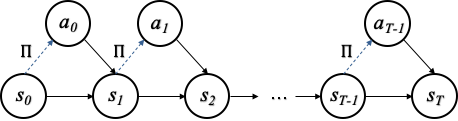
Figure 1: Finite horizon Markov decision process. This is a Markov decision process pictured as a Bayesian network (Pearl, 1998; Jordan et al., 1998). A finite horizon MDP comprises a finite sequence of states, indexed in time. The transition from one state to the next state depends on action. As such, for any given action sequence, the dynamics of the MDP form a Markov chain on state-space. In this fully observed setting, actions can be selected under a state-action policy, $\Pi$, indicated with a dashed line: this is a probabilistic mapping from state-space and time to actions.

Remark 2 (On the definition of reward).

More generally, the reward function can be taken to be dependent on the previous action and previous state: $R_{a}\left(s^{\prime}\mid s\right)$ is the reward received after transitioning from state $s$ to state $s^{\prime},$ due to action $a$ (Barto and Sutton, 1992; Stone, 2019). However, given an MDP with such a reward function, we can recover our simplified setting by defining a new MDP where the new states comprise the previous action, previous state, and current state in the original MDP. By inspection, the resulting reward function on the new MDP depends only on the current state (i.e., $R(s)$).

Remark 3 (Admissible actions).

In general, it is possible that only some actions can be taken at each state. In this case, one defines $\mathbb{A}_{s}$ to be the finite set of (allowable) actions from state $s\in\mathbb{S}$. All forthcoming results concerning MDPs can be extended to this setting.

To formalise what it means to choose actions in each state, we introduce the notion of a state-action policy.

Definition 4 (State-action policy).

A state-action policy $\Pi$ is a probability distribution over actions, that depends on the state that the agent occupies, and time. Explicitly,

$$\begin{split}\Pi:\mathbb{A}\times\mathbb{S}\times\mathbb{T}&\to[0,1]\\ (a,s,t)&\mapsto\Pi(a\mid s,t)\\ \forall(s,t)\in\mathbb{S}\times\mathbb{T}&:\sum_{a\in A}\Pi(a\mid s,t)=1.\end{split}$$

When $s_{t}=s$, we will write $\Pi(a\mid s_{t}):=\Pi(a\mid s,t)$. Note that the action at the temporal horizon $T$ is redundant, as no further reward can be reaped from the environment. Therefore, one often specifies state-action policies only up to time $T-1$, as $\Pi:\mathbb{A}\times\mathbb{S}\times\{0,\ldots,T-1\}\to[0,1]$. The state-action policy—as defined here—can be regarded as a generalisation of a deterministic state-action policy that assigns the probability of $1$ to an available action and $0$ otherwise.

Remark 5 (Conflicting terminologies: policy in active inference).

In active inference, a policy is defined as a sequence of actions indexed in time. To avoid terminological confusion, we use action sequences to denote policies under active inference.

At time $t$, the goal is to select an action that maximises future cumulative reward:

$$R(s_{t+1:T}):=\sum_{\tau=t+1}^{T}R(s_{\tau}).$$

Specifically, this entails following a state-action policy $\Pi$ that maximises the state-value function:

$$\begin{split}v_{\Pi}(s,t)&:=\mathbb{E}_{\Pi}[R(s_{t+1:T})\mid s_{t}=s]\end{split}$$

for any $(s,t)\in\mathbb{S}\times\mathbb{T}$. The state-value function scores the expected cumulative reward if the agent pursues state-action policy $\Pi$ from the state $s_{t}=s$. When the state $s_{t}=s$ is clear from context, we will often write $v_{\Pi}(s_{t}):=v_{\Pi}(s,t)$. Loosely speaking, we will call the expected reward the return.

Remark 6 (Notation $\mathbb{E}_{\Pi}$).

Whilst standard in RL (Barto and Sutton, 1992; Stone, 2019), the notation $\mathbb{E}_{\Pi}[R(s_{t+1:T})\mid s_{t}=s]$ can be confusing. It denotes the expected reward, under the transition probabilities of the MDP and a state-action policy $\Pi$

$$\mathbb{E}_{P(s_{t+1:T}\mid a_{t:T-1},s_{t}=s)\Pi(a_{t:T-1}\mid s_{t+1:T-1},s_{t}=s)}[R(s_{t+1:T})].$$

It is important to keep this correspondence in mind, as we will use both notations depending on context.

Remark 7 (Temporal discounting).

In infinite horizon MDPs (i.e., when $T$ is infinite), RL often seeks to maximise the discounted sum of rewards

$$\begin{split}v_{\Pi}(s,t)&:=\mathbb{E}_{\Pi}\left[\sum_{\tau=t}^{\infty}\gamma^{\tau-t}R(s_{\tau+1})\mid s_{t}=s\right],\end{split}$$

for a given temporal discounting term $\gamma\in(0,1)$ (Bertsekas and Shreve, 1996; Barto and Sutton, 1992; Kaelbling et al., 1998). In fact, temporal discounting is added to ensure that the infinite sum of future rewards converges to a finite value (Kaelbling et al., 1998). In finite horizon MDPs temporal discounting is not necessary so we set $\gamma=1$ (c.f.,  (Schmidhuber, 2010, 2006)).

To find the best state-action policies, we would like to rank them in terms of their return. We introduce a partial ordering such that a state-action policy is better than another if it yields a higher return in any situation:

$$\Pi\geq\Pi^{\prime}\iff\forall(s,t)\in\mathbb{S}\times\mathbb{T}:v_{\Pi}(s,t)\geq v_{\Pi^{\prime}}(s,t).$$

Similarly, a state-action policy $\Pi$ is strictly better than another $\Pi^{\prime}$ if it yields strictly higher returns:

$$\Pi>\Pi^{\prime}\iff\Pi\geq\Pi^{\prime}\text{ and }\exists(s,t)\in\mathbb{S}\times\mathbb{T}:v_{\Pi}(s,t)>v_{\Pi^{\prime}}(s,t).$$

2.2 Bellman optimal state-action policies

A state-action policy is Bellman optimal if it is better than all alternatives.

Definition 8 (Bellman optimality).

A state-action policy $\Pi^{*}$ is Bellman optimal if and only if it is better than all other state-action policies:

$$\Pi^{*}\geq\Pi,\forall\Pi.$$

In other words, it maximises the state-value function $v_{\Pi}(s,t)$ for any state $s$ at time $t$.

It is important to verify that this concept is not vacuous.

Proposition 9 (Existence of Bellman optimal state-action policies).

Given a finite horizon MDP as specified in Definition 1, there exists a Bellman optimal state-action policy $\Pi^{*}$.

A proof can be found in Appendix B.1. Note that uniqueness of the Bellman optimal state-action policy is not implied by Proposition 9; indeed, multiple Bellman optimal state-action policies may exist (Puterman, 2014; Bertsekas and Shreve, 1996).

Now that we know that Bellman optimal state-action policies exist, we can characterise them as a return-maximising action followed by a Bellman optimal state-action policy.

Proposition 10 (Characterisation of Bellman optimal state-action policies).

For a state-action policy $\Pi$, the following are equivalent:

1. $\Pi$ is Bellman optimal.

2. $\Pi$ is both

   1. Bellman optimal when restricted to $\{1,\ldots,T\}$. In other words, $\forall$ state-action policy $\Pi^{\prime}$ and $(s,t)\in\mathbb{S}\times\{1,\ldots T\}$

      $$v_{\Pi}(s,t)\geq v_{\Pi^{\prime}}(s,t).$$

   2. At time $0$, $\Pi$ selects actions that maximise return:

      $$\Pi(a\mid s,0)>0\iff a\in\arg\max_{a\in\mathbb{A}}\mathbb{E}_{\Pi}[R(s_{1:T})\mid s_{0}=s,a_{0}=a],\quad\forall s\in\mathbb{S}.$$ (1)

A proof can be found in Appendix B.2. Note that this characterisation offers a recursive way to construct Bellman optimal state-action policies by successively selecting the best action, as specified by (1), starting from $T$ and inducting backwards (Puterman, 2014).

2.3 Backward induction

Proposition 10 suggests a straightforward recursive algorithm to construct Bellman optimal state-action policies known as backward induction (Puterman, 2014). Backward induction has a long history. It was developed by the German mathematician Zermelo in 1913 to prove that chess has Bellman optimal strategies (Zermelo, 1913). In stochastic control, backward induction is one of the main methods for solving the Bellman equation (Miranda and Fackler, 2002; Adda and Cooper, 2003; Sargent, 2000). In game theory, the same method is used to compute sub-game perfect equilibria in sequential games (Fudenberg and Tirole, 1991).

Backward induction entails planning backwards in time, from a goal state at the end of a problem, by recursively determining the sequence of actions that enables reaching the goal. It proceeds by first considering the last time at which a decision might be made and choosing what to do in any situation at that time in order to get to the goal state. Using this information, one can then determine what to do at the second-to-last decision time. This process continues backwards until one has determined the best action for every possible situation or state at every point in time.

Proposition 11 (Backward induction: construction of Bellman optimal state-action policies).

Backward induction

$$\begin{split}\Pi(a\mid s,T-1)>0\iff a&\in\arg\max_{a\in\mathbb{A}}\mathbb{E}[R(s_{T})\mid s_{T-1}=s,a_{T-1}=a],\quad\forall s\in\mathbb{S}\\ \Pi(a\mid s,T-2)>0\iff a&\in\arg\max_{a\in\mathbb{A}}\mathbb{E}_{\Pi}[R(s_{T-1:T})\mid s_{T-2}=s,a_{T-2}=a],\quad\forall s\in\mathbb{S}\\ &\vdots\\ \Pi(a\mid s,0)>0\iff a&\in\arg\max_{a\in\mathbb{A}}\mathbb{E}_{\Pi}[R(s_{1:T})\mid s_{0}=s,a_{0}=a],\quad\forall s\in\mathbb{S}\\ \end{split}$$ (2)

defines a Bellman optimal state-action policy $\Pi$. Furthermore, this characterisation is complete: all Bellman optimal state-action policies satisfy the backward induction relation (2).

A proof can be found in Appendix B.3.

Example 1 (Intuition for backward induction).

To give a concrete example of this kind of planning, backward induction (2) would consider the actions below in the following order:

1. Desired goal: I would like to go to the grocery store,

2. Intermediate action: I need to drive to the store,

3. Current best action: I should put my shoes on.

Proposition 11 tells us that to be optimal with respect to reward maximisation, one must plan like backward induction. This will be central to our analysis of reward maximisation in active inference.

3 Active inference on finite horizon MDPs

We now turn to introducing active inference agents on finite horizon MDPs with known transition probabilities. We assume that the agent’s generative model of its environment is given by the previously defined finite horizon MDP (see Definition 1). We do not consider the case where the transitions have to be learned but comment on it in the Appendix A.2 (see also (Da Costa et al., 2020; Friston et al., 2016)).

In what follows, we fix a time $t\geq 0$ and suppose that the agent has been in states $s_{0},\ldots,s_{t}$. To ease notation, we let $\vec{s}:=s_{t+1:T},\vec{a}:=a_{t:T}$ be the future states and future actions. We define $Q$ to be the predictive distribution, which encodes the predicted future states and actions given that the agent is in state $s_{t}$

$$Q(\vec{s},\vec{a}\mid s_{t}):=\prod_{\tau=t}^{T-1}Q(s_{\tau+1}\mid a_{\tau},s_{\tau})Q(a_{\tau}\mid s_{\tau}).$$

3.1 Perception as inference

In active inference, perception entails inferences about future, past, and current states given observations and a sequence of actions. When states are partially observed, this is done through variational Bayesian inference by minimising a free energy functional (a.k.a. an evidence bound (Bishop, 2006; Beal, 2003; Wainwright and Jordan, 2007; Blei et al., 2017)).

In the MDP setting, past and current states are known, so it is only necessary to infer future states given the current state and action sequence $P(\vec{s}\mid\vec{a},s_{t})$. These posterior distributions $P(\vec{s}\mid\vec{a},s_{t})$ can be computed exactly in virtue of the fact that the transition probabilities of the MDP are known; hence variational inference becomes exact Bayesian inference.

$$\begin{split}Q(\vec{s}\mid\vec{a},s_{t})&:=P(\vec{s}\mid\vec{a},s_{t})=\prod_{\tau=t}^{T-1}P(s_{\tau+1}\mid s_{\tau},a_{\tau}).\end{split}$$ (3)

3.2 Planning as inference

Now that the agent has inferred future states given alternative action sequences, we must assess these alternative plans by examining the resulting state trajectories. The objective that active inference agents optimise—in order to select the best possible actions—is the expected free energy (Barp et al., 2022; Da Costa et al., 2020; Friston et al., 2021). Under active inference, agents minimise expected free energy in order to maintain themselves distributed according to a target distribution $C$ over the state-space $\mathbb{S}$ encoding the agent’s preferences.

Definition 12 (Expected free energy on MDPs).

On MDPs, the expected free energy of an action sequence $\vec{a}$ starting from $s_{t}$ is defined as (Barp et al., 2022):

$$G(\vec{a}\mid s_{t})=\operatorname{D_{KL}}[Q(\vec{s}\mid\vec{a},s_{t})\mid C(\vec{s})]$$ (4)

Therefore, minimising expected free energy corresponds to making the distribution over predicted states close to the distribution $C$ that encodes prior preferences. Note that the expected free energy in partially observed MDPs comprises an additional ambiguity term (see Section 5), which is dropped here as there is no ambiguity about observed states.

Since the expected free energy assesses the goodness of inferred future states under a course of action, we can refer to planning as inference (Attias, 2003; Botvinick and Toussaint, 2012). The expected free energy may be rewritten as

$$G(\vec{a}\mid s_{t})=\underbrace{\mathbb{E}_{Q(\vec{s}\mid\vec{a},s_{t})}[-\log C(\vec{s})]}_{\text{Expected surprise}}-\underbrace{\operatorname{H}[Q(\vec{s}\mid\vec{a},s_{t})]}_{\text{Entropy of future states}}$$ (5)

Hence, minimising expected free energy minimises the expected surprise of states according to $C$ and maximises the entropy of Bayesian beliefs over future states (a maximum entropy principle (Jaynes, 1957a), which is sometimes cast as keeping options open (Klyubin et al., 2008)).

Remark 13 (Numerical tractability).

The expected free energy is straightforward to compute using linear algebra. Given an action sequence $\vec{a}$, $C(\vec{s})$ and $Q(\vec{s}\mid\vec{a},s_{t})$ are categorical distributions over $\mathbb{S}^{T-t}$. Let their parameters be $\textbf{c},\textbf{s}_{\vec{a}}\in[0,1]^{\mid\mathbb{S}\mid(T-1)}$, where $\mid\cdot\mid$ denotes the cardinality of a set. Then the expected free energy reads

$$\begin{split}G(\vec{a}\mid s_{t})&=\textbf{s}_{\vec{a}}^{\operatorname{T}}(\log\textbf{s}_{\vec{a}}-\log\textbf{c}).\end{split}$$ (6)

Notwithstanding, (6) is expensive to evaluate repeatedly when all possible action sequences are considered. In practice, one can adopt a temporal mean field approximation over future states (Millidge et al., 2020a):

$$Q(\vec{s}\mid\vec{a},s_{t})\approx\prod_{\tau=t+1}^{T}Q(s_{\tau}\mid\vec{a},s_{t}),$$

which yields the simplified expression

$$G(\vec{a}\mid s_{t})\approx\sum_{\tau=t+1}^{T}\operatorname{D_{KL}}[Q(s_{\tau}\mid\vec{a},s_{t})\mid C(s_{\tau})].$$ (7)

Expression (7) is much easier to handle: for each action sequence $\vec{a}$, 1) one evaluates the summands sequentially $\tau=t+1,\ldots,T$, and 2) if and when the sum up to $\tau$ becomes significantly higher than the lowest expected free energy encountered during planning, $G(\vec{a}\mid s_{t})$ is set to an arbitrarily high value. Setting $G(\vec{a}\mid s_{t})$ to a high value is equivalent to pruning away unlikely trajectories. This bears some similarity to decision tree pruning procedures used in RL (Huys et al., 2012). It finesses exploration of the decision-tree in full depth and provides an Occam’s window for selecting action sequences.

Complementary approaches can help make planning tractable. For example, hierarchical generative models factorise decisions into multiple levels. By abstracting information at a higher-level, lower-levels entertain fewer actions (Friston et al., 2018)—which reduces the depth of the decision tree by orders of magnitude. Another approach is to use algorithms that search the decision-tree selectively, such as Monte-Carlo tree search (Silver et al., 2016; Champion et al., 2021a; Fountas et al., 2020; Maisto et al., 2021; Champion et al., 2021b), and amortising planning using artificial neural networks (i.e., learning to plan) (Çatal et al., 2020; Fountas et al., 2020; Sajid et al., 2021b).

4 Reward maximisation on MDPs through active inference

Here, we show how active inference solves the reward maximisation problem.

4.1 Reward maximisation as reaching preferences

From the definition of expected free energy (4), active inference on MDPs can be thought of as reaching and remaining at a target distribution $C$ over state-space.

The idea that underwrites this section is that when the stationary distribution has all of its mass on reward maximising states, the agent will maximise reward. To illustrate this, we define a preference distribution $C_{\beta},\beta>0$ over state-space $\mathbb{S}$, such that preferred states are rewarding states

$$\begin{split}C_{\beta}(\sigma)&:=\frac{\exp\beta R(\sigma)}{\sum_{\varsigma\in\mathbb{S}}\exp\beta R(\varsigma)}\propto\exp(\beta R(\sigma)),\quad\forall\sigma\in\mathbb{S}\\ \iff-\log C_{\beta}(\sigma)&=-\beta R(\sigma)-c(\beta),\quad\forall\sigma\in\mathbb{S},\text{ for some }c(\beta)\in\mathbb{R}\text{ constant w.r.t }\sigma.\end{split}$$

The (inverse temperature) parameter $\beta>0$ scores how motivated the agent is to occupy reward maximising states. Note that states $s\in\mathbb{S}$ that maximise the reward $R(s)$ maximise $C_{\beta}(s)$ and minimise $-\log C_{\beta}(s)$ for any $\beta>0$.

Using the additive property of the reward function, we can extend $C_{\beta}$ to a probability distribution over trajectories $\vec{\sigma}:=(\sigma_{1},\ldots,\sigma_{T})\in\mathbb{S}^{T}$. Specifically, $C_{\beta}$ scores to what extent a trajectory is preferred over another trajectory:

$$\begin{split}C_{\beta}(\vec{\sigma})&:=\frac{\exp\beta R(\vec{\sigma})}{\sum_{\vec{\varsigma}\in\mathbb{S}^{T}}\exp\beta R(\vec{\varsigma})}=\prod_{\tau=1}^{T}\frac{\exp\beta R(\sigma_{\tau})}{\sum_{\varsigma\in\mathbb{S}}\exp\beta R(\varsigma)}=\prod_{\tau=1}^{T}C_{\beta}(\sigma_{\tau}),\quad\forall\vec{\sigma}\in\mathbb{S}^{T}\\ \iff&-\log C_{\beta}(\vec{\sigma})=-\beta R(\vec{\sigma})-c^{\prime}(\beta)=-\sum_{\tau=1}^{T}\beta R(\sigma_{\tau})-c^{\prime}(\beta),\quad\forall\vec{\sigma}\in\mathbb{S}^{T},\end{split}$$ (8)

where $c^{\prime}(\beta):=c(\beta)T\in\mathbb{R}$ is constant w.r.t $\vec{\sigma}$.

When the preferences are defined in this way, the zero-temperature limit $\beta\to+\infty$ is the case where the preferences $C_{\beta}$ are non-zero only for states or trajectories that maximise reward. In this case, $\lim_{\beta\to+\infty}C_{\beta}$ is a uniform mixture of Dirac distributions over reward maximising trajectories:

$$\begin{split}\lim_{\beta\to+\infty}C_{\beta}&\propto\sum_{\vec{s}\in I^{T-t}}\operatorname{Dirac}_{\vec{s}}\\ I&:=\arg\max_{s\in\mathbb{S}}R(s).\end{split}$$ (9)

This is because, for a reward maximising state $\sigma$, $\exp(\beta R(\sigma))$ will converge to $+\infty$ more quickly than $\exp(\beta R(\sigma^{\prime}))$ for a non-reward maximising state $\sigma^{\prime}$. Since $C_{\beta}$ is constrained to be normalised to $1$ (as it is a probability distribution), $C_{\beta}(\sigma^{\prime})\xrightarrow{\beta\to+\infty}0$. Hence, in the limit $\beta\to+\infty$, $C_{\beta}$ is non-zero (and uniform) only on reward maximising states.

We now show how reaching preferred states can be formulated as reward maximisation:

Lemma 14.

The sequence of actions that minimises expected free energy also maximises expected reward in the zero temperature limit $\beta\to+\infty$ (9):

$$\lim_{\beta\to+\infty}\arg\min_{\vec{a}}G(\vec{a}\mid s_{t})\subseteq\arg\max_{\vec{a}}\mathbb{E}_{Q(\vec{s}\mid\vec{a},s_{t})}[R(\vec{s})]$$

Furthermore, of those action sequences that maximise expected reward, the expected free energy minimisers will be those that maximise the entropy of future states $\operatorname{H}[Q(\vec{s}\mid\vec{a},s_{t})]$.

A proof can be found in Appendix B.4. In the zero temperature limit $\beta\to+\infty$, minimising expected free energy corresponds to choosing the action sequence $\vec{a}$ such that $Q(\vec{s}\mid\vec{a},s_{t})$ has most mass on reward maximising states or trajectories (see Figure 2). Of those reward maximising candidates, the minimiser of expected free energy maximises the entropy of future states $\operatorname{H}[Q(\vec{s}\mid\vec{a},s_{t})]$, thus leaving options open.

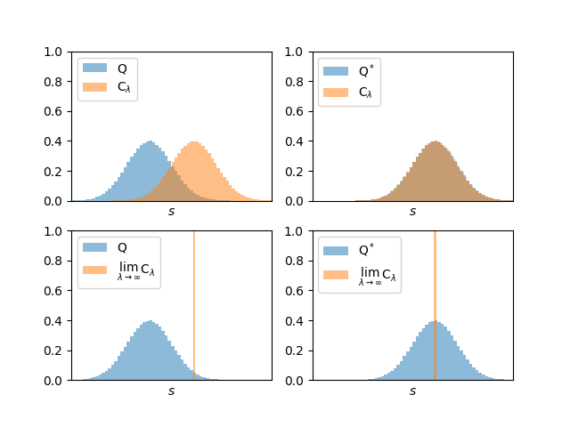
Figure 2: Reaching preferences and the zero temperature limit. We illustrate how active inference selects actions such that $Q(\vec{s}\mid\vec{a},s_{t})$ most closely matches the preference distribution $C_{\beta}$ (top-right). In this example, the discrete state-space is a discretisation of a continuous interval in $\mathbb{R}$, and the preferences and predictive distributions over states have a Gaussian shape. The predictive distribution $Q$ is assumed to have a fixed variance with respect to action sequences, such that the only parameter that can be optimised by action selection is its mean. Crucially, in the zero temperature limit (9), $\lim_{\beta\to+\infty}C_{\beta}$ becomes a Dirac distribution over the reward maximising state (bottom). Thus, minimising expected free energy corresponds to selecting the action such that the predicted states assign most mass to the reward maximising state (bottom-right). $Q^{*}:=Q(\vec{s}\mid\vec{a}^{*},s_{t})$ denotes the predictive distribution over states given the action sequence that minimises expected free energy $\vec{a}^{*}=\arg\min_{\vec{a}}G(\vec{a}\mid s_{t})$.

4.2 Reward maximisation on MDPs with a temporal horizon of $1$

In this section, we first consider the case of a single-step decision problem (i.e., a temporal horizon of $T=1$) and demonstrate how the standard active inference scheme maximises reward on this problem in the limit $\beta\to+\infty$. This will act as an important building block for when we subsequently consider more general multi-step decision problems.

The standard decision-making procedure in active inference consists of assigning each action sequence with a probability given by the softmax of the negative expected free energy (Da Costa et al., 2020; Friston et al., 2017a; Barp et al., 2022)

$$Q(\vec{a}\mid s_{t})\propto\exp(-G(\vec{a}\mid s_{t})).$$

Agents then select the most likely action under this distribution

$$a_{t}\in\arg\max_{a\in\mathbb{A}}Q(a\mid s_{t}) =\arg\max_{a\in\mathbb{A}}\sum_{\vec{a}}Q(a\mid\vec{a})Q(\vec{a}\mid s_{t})$$

$$=\arg\max_{a\in\mathbb{A}}\sum_{\vec{a}}Q(a\mid\vec{a})\exp(-G(\vec{a}\mid s_{t})) =\arg\max_{a\in\mathbb{A}}\sum_{\begin{subarray}{c}\vec{a}\\ \left(\vec{a}\right)_{t}=a\end{subarray}}\exp(-G(\vec{a}\mid s_{t})).$$

In summary, this scheme selects the first action within action sequences that, on average, maximise their exponentiated negative expected free energies. As a corollary, if the first action is in a sequence with a very low expected free energy, this adds an exponentially large contribution to the selection of this particular action. We summarise this scheme in Table 1.

Process	Computation
Perceptual inference	$Q(\vec{s}\mid\vec{a},s_{t})=P(\vec{s}\mid\vec{a},s_{t})=\prod_{\tau=t}^{T-1}P(s_{\tau+1}\mid s_{\tau},a_{\tau})$
Planning as inference	$G(\vec{a}\mid s_{t})=\operatorname{D_{KL}}[Q(\vec{s}\mid\vec{a},s_{t})\mid C(\vec{s})]$
Decision-making	$Q(\vec{a}\mid s_{t})\propto\exp(-G(\vec{a}\mid s_{t}))$
Action selection	$a_{t}\in\arg\max_{a\in\mathbb{A}}\left[Q(a_{t}=a\mid s_{t})=\sum_{\vec{a}}Q(a_{t}=a\mid\vec{a})Q(\vec{a}\mid s_{t})\right]$

Table 1: Standard active inference scheme on finite horizon MDPs (Barp et al., 2022).

Theorem 15.

In MDPs with known transition probabilities and in the zero temperature limit $\beta\to+\infty$ (9), the scheme of Table 1

$$a_{t}\in\lim_{\beta\to+\infty}\arg\max_{a\in\mathbb{A}}\sum_{\begin{subarray}{c}\vec{a}\\ \left(\vec{a}\right)_{t}=a\end{subarray}}\exp(-G(\vec{a}\mid s_{t})),\qquad G(\vec{a}\mid s_{t})=\operatorname{D_{KL}}[Q(\vec{s}\mid\vec{a},s_{t})\mid C_{\beta}(\vec{s})]$$ (10)

is Bellman optimal for the temporal horizon $T=1$.

A proof can be found in Appendix B.5. Importantly, the standard active inference scheme (10) falls short in terms of Bellman optimality on planning horizons greater than one; this rests upon the fact that it does not coincide with backward induction. Recall that backward induction offers a complete description of Bellman optimal state-action policies (Proposition 11). In contrast, active inference plans by adding weighted expected free energies of each possible future course of action. In other words, unlike backward induction, it considers future courses of action beyond the subset that will subsequently minimise expected free energy, given subsequently encountered states.

4.3 Reward maximisation on MDPs with finite temporal horizons

To achieve Bellman optimality on finite temporal horizons, we turn to the expected free energy of an action given future actions that also minimise expected free energy. To do this we can write the expected free energy recursively, as the immediate expected free energy, plus the expected free energy that one would obtain by subsequently selecting actions that minimise expected free energy (Friston et al., 2021). The resulting scheme consists of minimising an expected free energy defined recursively, from the last time step to the current timestep. In finite horizon MDPs, this reads

$$G(a_{T-1}\mid s_{T-1}) =\operatorname{D_{KL}}[Q(s_{T}\mid a_{T-1},s_{T-1})\mid C_{\beta}(s_{T})]$$

$$G(a_{\tau}\mid s_{\tau}) =\operatorname{D_{KL}}[Q(s_{\tau+1}\mid a_{\tau},s_{\tau})\mid C_{\beta}(s_{\tau+1})]$$

$$+\mathbb{E}_{Q(a_{\tau+1},s_{\tau+1}\mid a_{\tau},s_{\tau})}[G(a_{\tau+1}\mid s_{\tau+1})],\quad\tau=t,\ldots,T-2,$$

where, at each time-step, actions are chosen to minimise expected free energy

$$Q(a_{\tau+1}\mid s_{\tau+1})>0\iff a_{\tau+1}\in\arg\min_{a\in\mathbb{A}}G(a\mid s_{\tau+1}).$$ (11)

To make sense of this formulation, we unravel the recursion

$$\begin{split}G(a_{t}\mid s_{t})&=\operatorname{D_{KL}}[Q(s_{t+1}\mid a_{t},s_{t})\mid C_{\beta}(s_{t+1})]+\mathbb{E}_{Q(a_{t+1},s_{t+1}\mid a_{t},s_{t})}[G(a_{t+1}\mid s_{t+1})]\\ &=\operatorname{D_{KL}}[Q(s_{t+1}\mid a_{t},s_{t})\mid C_{\beta}(s_{t+1})]+\mathbb{E}_{Q(a_{t+1},s_{t+1}\mid a_{t},s_{t})}\left[\operatorname{D_{KL}}[Q(s_{t+2}\mid a_{t+1},s_{t+1})\mid C_{\beta}(s_{t+2})]\right]\\ &+\mathbb{E}_{Q(a_{t+1:t+2},s_{t+1:t+2}\mid a_{t},s_{t})}[G(a_{t+2}\mid s_{t+2})]\\ &=\ldots=\mathbb{E}_{Q(\vec{a},\vec{s}\mid a_{t},s_{t})}\sum_{\tau=t}^{T-1}\operatorname{D_{KL}}[Q(s_{\tau+1}\mid a_{\tau},s_{\tau})\mid C_{\beta}(s_{\tau+1})]\\ &=\mathbb{E}_{Q(\vec{a},\vec{s}\mid a_{t},s_{t})}\operatorname{D_{KL}}[Q(\vec{s}\mid\vec{a},s_{t})\mid C_{\beta}(\vec{s})],\end{split}$$ (12)

which shows that this expression is exactly the expected free energy under action $a_{t}$, if one is to pursue future actions that minimise expected free energy (11). We summarise this ’sophisticated inference’ scheme in Table 2.

Process	Computation
Perceptual inference	$Q(s_{\tau+1}\mid a_{\tau},s_{\tau})=P(s_{\tau+1}\mid a_{\tau},s_{\tau})$
Planning as inference	$G(a_{\tau}\mid s_{\tau})=\operatorname{D_{KL}}[Q(s_{\tau+1}\mid a_{\tau},s_{\tau})\mid C_{\beta}(s_{\tau+1})]\ldots$
	$\qquad\qquad\ldots+\mathbb{E}_{Q(a_{\tau+1},s_{\tau+1}\mid a_{\tau},s_{\tau})}[G(a_{\tau+1}\mid s_{\tau+1})]$
Decision-making	$Q(a_{\tau}\mid s_{\tau})>0\iff a_{\tau}\in\arg\min_{a\in\mathbb{A}}G(a\mid s_{\tau})$
Action selection	$a_{t}\sim Q(a_{t}\mid s_{t})$

Table 2: Sophisticated active inference scheme on finite horizon MDPs (Friston et al., 2021).

The crucial improvement over the standard active inference scheme (Table 1) is that planning is now performed based on subsequent counterfactual actions that minimise expected free energy, as opposed to considering all future courses of action. Translating this into the language of state-action policies yields $\forall s\in\mathbb{S}$

$$\begin{split}a_{T-1}(s)&\in\arg\min_{a\in\mathbb{A}}G(a\mid s_{T-1}=s)\\ a_{T-2}(s)&\in\arg\min_{a\in\mathbb{A}}G(a\mid s_{T-2}=s)\\ &\vdots\\ a_{1}(s)&\in\arg\min_{a\in\mathbb{A}}G(a\mid s_{1}=s)\\ a_{0}(s)&\in\arg\min_{a\in\mathbb{A}}G(a\mid s_{0}).\\ \end{split}$$ (13)

Equation (13) is strikingly similar to the backward induction algorithm (Proposition 11), and indeed we recover backward induction in the limit $\beta\to+\infty$.

Theorem 16 (Backward induction as active inference).

In MDPs with known transition probabilities, and in the zero temperature limit $\beta\to+\infty$ (9), the scheme of Table 2

$$\begin{split}Q(a_{\tau}\mid s_{\tau})>0&\iff a_{t}\in\lim_{\beta\to+\infty}\arg\min_{a\in\mathbb{A}}G(a\mid s_{\tau})\\ G(a_{\tau}\mid s_{\tau})&=\operatorname{D_{KL}}[Q(s_{\tau+1}\mid a_{\tau},s_{\tau})\mid C_{\beta}(s_{\tau+1})]+\mathbb{E}_{Q(a_{\tau+1},s_{\tau+1}\mid a_{\tau},s_{\tau})}[G(a_{\tau+1}\mid s_{\tau+1})]\\ \end{split}$$ (14)

is Bellman optimal on any finite temporal horizon as it coincides with the backward induction algorithm from Proposition 11. Furthermore, if there are multiple actions that maximise future reward, those that are selected by active inference also maximise the entropy of future states $\operatorname{H}[Q(\vec{s}\mid\vec{a},a,s_{0})]$.

Note that maximising the entropy of future states keeps the agent’s options open (Klyubin et al., 2008) in the sense of committing the least to a specified sequence of states. A proof of Theorem 16 can be found in Appendix B.6.

5 Generalisation to POMDPs

Partially observable Markov decision processes (POMDPs) generalise MDPs in that the agent observes a modality $o_{t}$, which carries incomplete information about the current state $s_{t}$, as opposed to the current state itself.

Definition 17 (Finite horizon POMDP).

A finite horizon POMDP is an MDP (see Definition 1) with the following additional data:

• $\mathbb{O}$ a finite set of observations.

• $P(o_{t}=o\mid s_{t}=s)$ is the probability that the state $s\in\mathbb{S}$ at time $t$ will lead to the observation $o\in\mathbb{O}$ at time $t$. $o_{t}$ are random variables over $\mathbb{O}$ that correspond to the observation being sampled at time $t=0,...,T$.

5.1 Active inference on finite horizon POMDPs

We briefly introduce active inference agents on finite horizon POMDPs with known transition probabilities (for more details, see (Da Costa et al., 2020; Smith et al., 2022a; Parr et al., 2022)). We assume that the agent’s generative model of its environment is given by the previously defined POMDP (Definition 17).

Let $\vec{s}:=s_{0:T},\vec{a}:=a_{0:T-1}$ be all states and actions (past, present, and future), let $\tilde{o}:=o_{0:t}$ be the observations available up to time $t$, and $\vec{o}:=o_{t+1:T}$ be the future observations. The agent has a predictive distribution over states given actions

$$Q(\vec{s}\mid\vec{a},\tilde{o}):=\prod_{\tau=0}^{T-1}Q(s_{\tau+1}\mid a_{\tau},s_{\tau},\tilde{o}).$$

that is continuously updated following new observations.

5.1.1 Perception as inference

In active inference, perception entails inferences about (past, present, and future) states given observations and a sequence of actions. When states are partially observed, the posterior distribution $P(\vec{s}\mid\vec{a},\tilde{o})$ is intractable to compute directly. Thus, one approximates it by optimising a variational free energy functional $F_{\vec{a}}$ (a.k.a. an evidence bound (Bishop, 2006; Beal, 2003; Wainwright and Jordan, 2007; Blei et al., 2017)) over a space of probability distributions $Q(\cdot\mid\vec{a},\tilde{o})$ called the variational family

$$\begin{split}P(\vec{s}\mid\vec{a},\tilde{o})=\arg\min_{Q}F_{\vec{a}}[Q(\vec{s}\mid\vec{a},\tilde{o})]&=\arg\min_{Q}\operatorname{D_{KL}}[Q(\vec{s}\mid\vec{a},\tilde{o})\mid P(\vec{s}\mid\vec{a},\tilde{o})]\\ F_{\vec{a}}[Q(\vec{s}\mid\vec{a},\tilde{o})]&:=\mathbb{E}_{Q(\vec{s}\mid\vec{a},\tilde{o})}[\log Q(\vec{s}\mid\vec{a},\tilde{o})-\log P(\tilde{o},\vec{s}\mid\vec{a})].\end{split}$$ (15)

Here, $P(\tilde{o},\vec{s}\mid\vec{a})$ is the POMDP, which is supplied to the agent, and $P(\vec{s}\mid\vec{a},\tilde{o})$. When the free energy minimum (15) is reached, the inference is exact

$$Q(\vec{s}\mid\vec{a},\tilde{o})=P(\vec{s}\mid\vec{a},\tilde{o}).$$ (16)

For numerical tractability, the variational family may be constrained to a parametric family of distributions, in which case equality is not guaranteed

$$Q(\vec{s}\mid\vec{a},\tilde{o})\approx P(\vec{s}\mid\vec{a},\tilde{o}).$$ (17)

5.1.2 Planning as inference

The objective that active inference minimises in order the select the best possible courses of action is the expected free energy (Barp et al., 2022; Da Costa et al., 2020; Friston et al., 2021). In POMDPs, the expected free energy reads (Barp et al., 2022)

$$\begin{split}G(\vec{a}\mid\tilde{o})&=\underbrace{\operatorname{D_{KL}}[Q(\vec{s}\mid\vec{a},\tilde{o})\mid C_{\beta}(\vec{s})]}_{\text{Risk}}+\underbrace{\mathbb{E}_{Q(\vec{s}\mid\vec{a},\tilde{o})}\operatorname{H}[P(\vec{o}\mid\vec{s})]}_{\text{Ambiguity}}.\\ \end{split}$$

The expected free energy on POMDPs is the expected free energy on MDPs plus an extra term called ambiguity. This ambiguity term accommodates the uncertainty implicit in partially observed problems. The reason that this resulting functional is called expected free energy is because it comprises a relative entropy (risk) and expected energy (ambiguity). The expected free energy objective subsumes several decision-making objectives that predominate in statistics, machine learning, and psychology, which confers it with several useful properties when simulating behaviour (see Figure 3 for details).

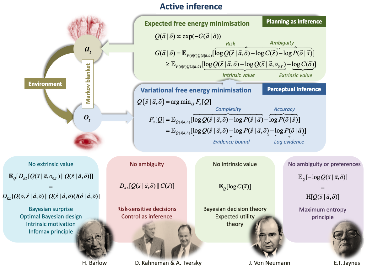
Figure 3: Active inference. The top panels illustrate the perception-action loop in active inference, in terms of minimisation of variational and expected free energy. The lower panels illustrate how expected free energy relates to several descriptions of behaviour that predominate in the psychological, machine learning, and economics. These descriptions are disclosed when one removes particular terms from the objective. For example, if we ignore extrinsic value, we are left with intrinsic value, variously known as expected information gain (MacKay, 2003; Lindley, 1956). This underwrites intrinsic motivation in machine learning and robotics (Barto et al., 2013; Oudeyer and Kaplan, 2007; Deci and Ryan, 1985) and expected Bayesian surprise in visual search (Itti and Baldi, 2009; Sun et al., 2011) and the organisation of our visual apparatus (Linsker, 1990; Optican and Richmond, 1987; Barlow, 1961, 1974). In the absence of ambiguity, we are left with minimising risk, which corresponds to aligning predicted states to preferred states. This leads to risk averse decisions in behavioural economics (Kahneman and Tversky, 1979) and formulations of control as inference in engineering such as KL control  (van den Broek et al., 2010). If we then remove intrinsic value, we are left with expected utility in economics (Von Neumann and Morgenstern, 1944) that underwrites RL and behavioural psychology (Barto and Sutton, 1992). Bayesian formulations of maximising expected utility under uncertainty are also the basis of Bayesian decision theory (Berger, 1985). Finally, if we only consider a fully observed environment with no preferences, minimising expected free energy corresponds to a maximum entropy principle over future states (Jaynes, 1957a, b). Note that here $C(o)$ denotes the preferences over observations derived from the preferences over states. These are related by $P(o\mid s)C(s)=P(s\mid o)C(o)$.

5.2 Maximising reward on POMDPs

Crucially, our reward maximisation results translate to the POMDP case. To make this explicit, we rehearse Lemma 14 in the context of POMDPs.

Proposition 18 (Reward maximisation on POMDPs).

In POMDPs with known transition probabilities, provided that the free energy minimum is reached (16), the sequence of actions that minimises expected free energy also maximises expected reward in the zero temperature limit $\beta\to+\infty$ (9):

$$\lim_{\beta\to+\infty}\arg\min_{\vec{a}}G(\vec{a}\mid\tilde{o})\subseteq\arg\max_{\vec{a}}\mathbb{E}_{Q(\vec{s}\mid\vec{a},\tilde{o})}[R(\vec{s})].$$

Furthermore, of those action sequences that maximise expected reward, the expected free energy minimisers will be those that maximise the entropy of future states minus the (expected) entropy of outcomes given states $\operatorname{H}[Q(\vec{s}\mid\vec{a},\tilde{o})]-\mathbb{E}_{Q(\vec{s}\mid a_{t},\tilde{o})}\operatorname{H}[P(\vec{o}\mid\vec{s})]]$.

From Proposition 18 we see that if there are multiple maximise reward action sequences, those that are selected maximise

$$\underbrace{\operatorname{H}[Q(\vec{s}\mid\vec{a},\tilde{o})]}_{\text{Entropy of future states}}-\underbrace{\mathbb{E}_{Q(\vec{s}\mid a_{t},\tilde{o})}[\operatorname{H}[P(\vec{o}\mid\vec{s})]]}_{\text{Entropy of observations given future states}}.$$

In other words, they least commit to a prespecified sequence of future states and ensure that their expected observations are maximally informative of states. Of course, when inferences are inexact, the extent to which Proposition 18 holds depends upon the accuracy of the approximation (17). A proof of Proposition 18 can be found in Appendix B.7.

The schemes of Table 1 & 2 exist in the POMDP setting, (e.g., (Barp et al., 2022) and (Friston et al., 2021), respectively). Thus, in POMDPs with known transition probabilities, provided that inferences are exact (16) and in the zero temperature limit $\beta\to+\infty$ (9), standard active inference (Barp et al., 2022) maximises reward on temporal horizons of $1$ but not beyond, and a recursive scheme such as sophisticated active inference (Friston et al., 2021) maximises reward on finite temporal horizons. Note that, for computational tractability, the sophisticated active inference scheme presented in (Friston et al., 2021) does not generally perform exact inference; thus, the extent to which it will maximise reward in practice will depend upon the accuracy of its inferences. Nevertheless, our results indicate that sophisticated active inference will vastly outperform standard active inference in most reward maximisation tasks.

6 Discussion

In this paper, we have examined a specific notion of optimality; namely, Bellman optimality; defined as selecting actions to maximise future expected rewards. We demonstrated how and when active inference is Bellman optimal on finite horizon POMDPs with known transition probabilities and reward function.

These results highlight important relationships between active inference, stochastic control, and RL, as well as conditions under which they would and would not be expected to behave similarly (e.g., environments with multiple reward-maximising trajectories, those affording ambiguous observations, etc.). We refer the reader to Appendix A for a broader discussion of the relationship between active inference and reinforcement learning.

6.1 Decision-making beyond reward maximisation

More broadly, it is important to ask if reward maximisation is the right objective underwriting intelligent decision-making? This is an important question for decision neuroscience. That is, do humans optimise a reward signal, expected free energy, or other planning objectives. This can be addressed by comparing the evidence for these competing hypotheses based on empirical data (e.g., see (Smith et al., 2020d, 2022b, 2021b, 2021c)). Current empirical evidence suggests that humans are not purely reward-maximising agents: they also engage in both random and directed exploration (Daw et al., 2006; Mirza et al., 2018; Wilson et al., 2014; Gershman, 2018; Schulz and Gershman, 2019; Wilson et al., 2021; Xu et al., 2021) and keep their options open (Schwartenbeck et al., 2015b). As we have illustrated, active inference implements a clear form of directed exploration through minimising expected free energy. Although not covered in detail here, active inference can also accommodate random exploration by sampling actions from the posterior belief over action sequences, as opposed to selecting the most likely action as presented in Tables 1 and 2.

Note that behavioural evidence favouring models that do not solely maximise reward within reward maximisation tasks—i.e., where "maximise reward" is the explicit instruction—is not a contradiction. Rather, gathering information about the environment (exploration) generally helps to reap more reward in the long run, as opposed to greedily maximising reward based on imperfect knowledge (Sajid et al., 2021a; Cullen et al., 2018). This observation is not new and many approaches to simulating adaptive agents employed today differ significantly from their reward maximising antecedents (Appendix A.3).

6.2 Learning

When the transition probabilities or reward function are unknown to the agent, the problem becomes one of reinforcement learning (RL) (Shoham et al., 2003) as opposed to stochastic control. Although we did not explicitly consider it above, this scenario can be accommodated by active inference by simply equipping the generative model with a prior, and updating the model via variational Bayesian inference to best fit observed data. Depending on the specific learning problem and generative model structure, this can involve updating the transition probabilities and/or the target distribution $C$. In POMDPs it can also involve updating the probabilities of observations under each state. We refer to Appendix A.2 for discussion of reward learning through active inference and connections to representative RL approaches, and (Da Costa et al., 2020; Friston et al., 2016) for learning transition probabilities through active inference.

6.3 Scaling active inference

When comparing RL and active inference approaches generally, one outstanding issue for active inference is whether it can be scaled up to solve the more complex problems currently handled by RL in machine learning contexts (Çatal et al., 2020; Tschantz et al., 2019; Millidge, 2020; Çatal et al., 2021; Fountas et al., 2020; Mazzaglia et al., 2021). This is an area of active research.

One important issue along these lines is that planning ahead by evaluating all or many possible sequences of actions is computationally prohibitive in many applications. Three complementary solutions that have emerged are: 1) employing hierarchical generative models that factorise decisions into multiple levels and reduce the size of the decision tree by orders of magnitude (Friston et al., 2018; Çatal et al., 2021; Parr et al., 2021), 2) efficiently searching the decision tree using algorithms like Monte Carlo tree search (Silver et al., 2016; Fountas et al., 2020; Maisto et al., 2021; Champion et al., 2021a, b), and 3) amortising planning using artificial neural networks (Çatal et al., 2020; Fountas et al., 2020; Sajid et al., 2021b).

Another issue rests upon learning the generative model. Active inference may readily learn the parameters of a generative model; however, more work needs to be done on devising algorithms for learning the structure of generative models themselves (Smith et al., 2020c; Friston et al., 2017b). This is an important research problem in generative modelling, called Bayesian model selection or structure learning (Gershman and Niv, 2010; Tervo et al., 2016).

Note that these issues are not unique to active inference. Model-based RL algorithms deal with the same combinatorial explosion when evaluating decision trees, which is one primary motivation for developing efficient model-free RL algorithms. However, other heuristics have also been developed for efficiently searching and pruning decision trees in model-based RL, e.g., (Huys et al., 2012; Lally et al., 2017). Furthermore, model-based RL suffers the same limitation regarding learning generative model structure. Yet, RL may have much to offer active inference in terms of efficient implementation and the identification of methods to scale to more complex applications (Mazzaglia et al., 2021; Fountas et al., 2020).

7 Conclusion

In summary, we have shown that under the specification that the active inference agent prefers maximising reward (9):

1. On finite horizon POMDPs with known transition probabilities, the objective optimised for action selection in active inference (i.e., expected free energy) produces reward maximising action sequences when state-estimation is exact. When there are multiple reward maximising candidates, this selects those sequences that maximise the entropy of future states—thereby keeping options open—and that minimise the ambiguity of future observations so that they are are maximally informative. More generally, the extent to which action sequences will be reward maximising will depend on the accuracy of state-estimation.

2. The standard active inference scheme (e.g.,  (Barp et al., 2022)) produces Bellman optimal actions for planning horizons of $1$ when state-estimation is exact, but not beyond.

3. A sophisticated active inference scheme (e.g., (Friston et al., 2021)) produces Bellman optimal actions on any finite planning horizon when state-estimation is exact. Furthermore, this scheme generalises the well-known backward induction algorithm from dynamic programming to partially observed environments. Note that, for computational efficiency, the scheme presented in (Friston et al., 2021) does not generally perform exact state-estimation; thus, the extent to which it will maximise reward in practice will depend upon the accuracy of its inferences. Nevertheless, it is clear from our results that sophisticated active inference will vastly outperform standard active inference in most reward maximisation tasks.

Note that, for computational tractability, the sophisticated active inference scheme presented in (Friston et al., 2021) does not generally perform exact inference; thus, the extent to which it will maximise reward in practice will depend upon the accuracy of its inferences. Nevertheless, it is clear from these results that sophisticated active inference will vastly outperform standard active inference in most reward maximisation tasks.

Funding information

LD is supported by the Fonds National de la Recherche, Luxembourg (Project code: 13568875). NS is funded by the Medical Research Council (MR/S502522/1) and 2021-2022 Microsoft PhD Fellowship. KF is supported by funding for the Wellcome Centre for Human Neuroimaging (Ref: 205103/Z/16/Z), a Canada-UK Artificial Intelligence Initiative (Ref: ES/T01279X/1) and the European Union’s Horizon 2020 Framework Programme for Research and Innovation under the Specific Grant Agreement No. 945539 (Human Brain Project SGA3). RS is supported by the William K. Warren Foundation, the Well-Being for Planet Earth Foundation, the National Institute for General Medical sciences (P20GM121312), and the National Institute of Mental Health (R01MH123691). This publication is based on work partially supported by the EPSRC Centre for Doctoral Training in Mathematics of Random Systems: Analysis, Modelling and Simulation (EP/S023925/1).

Author contributions

LD: conceptualisation, proofs, writing – first draft, review and editing. NS, TP, KF, RS: conceptualisation, writing – review and editing.

A Active inference and reinforcement learning

This paper considered how active inference can solve the stochastic control problem. In this appendix, we discuss the broader relationship between active inference and RL.

Loosely speaking, RL is the field of methodologies and algorithms that learn reward-maximising actions from data and seek to maximise reward in the long run. Because RL is a data-driven field, algorithms are selected based on how well they perform on benchmark problems. This has produced a plethora of diverse algorithms, many designed to solve specific problems, each with their own strengths and limitations. This makes RL difficult to characterise as a whole. Thankfully, many approaches to model-based RL and control can be traced back to approximating the optimal solution to the Bellman equation (Bellman and Dreyfus, 2015; Bertsekas and Shreve, 1996) (although this may become computationally intractable in high-dimensions (Barto and Sutton, 1992)). Our results showed how and when decisions under active inference and such RL approaches are similar.

This appendix discusses how active inference and RL relate and differ more generally. Their relationship has become increasingly important to understand, as a growing body of research has begun to 1) compare the performance of active inference and RL models in simulated environments (Sajid et al., 2021a; Cullen et al., 2018; Millidge, 2020), 2) apply active inference to model human behaviour on reward learning tasks (Smith et al., 2022b, 2021b, 2021c, 2020d), and 3) consider the complementary predictions and interpretations they each offer in computational neuroscience, psychology, and psychiatry (Schwartenbeck et al., 2019, 2015a; Tschantz et al., 2020b; Cullen et al., 2018; Huys et al., 2012).

A.1 Main differences between active inference and reinforcement learning

Philosophy.

Active inference and RL differ profoundly in their philosophy. RL derives from the normative principle of maximising reward (Barto and Sutton, 1992), while active inference describes systems that maintain their structural integrity over time (Friston et al., 2022; Barp et al., 2022). Despite this difference, there are many practical similarities between these frameworks. For example, recall that behaviour in active inference is completely determined by the agent’s preferences, determined as priors in their generative model. Crucially, log priors can be interpreted as reward functions and vice-versa, which is how behaviour under RL and active inference can be related.

Model based and model free.

Active inference agents always embody a generative (i.e., forward) model of their environment, while RL comprises both model-based algorithms and simpler model-free algorithms. In brief, ’model-free’ means that agents learn a reward-maximising state-action mapping, based on updating cached state-action pair values, through initially random actions that do not consider future state transitions. In contrast, model-based RL algorithms attempt to extend stochastic control approaches by learning the dynamics and reward function from data. Recall that stochastic control calls on strategies that evaluate different actions on a carefully handcrafted forward model of dynamics (i.e., known transition probabilities) to finally execute the reward-maximising action. Under this terminology, all active inference agents are model-based.

Modelling exploration.

Exploratory behaviour—which can improve reward maximisation in the long run—is implemented differently in the two approaches. In most cases, RL implements a simple form of exploration by incorporating randomness in decision-making (Tokic and Palm, 2011; Wilson et al., 2014), where the level of randomness may or may not change over time as a function of uncertainty. In other cases, RL incorporates ad-hoc information bonuses in the reward function or other decision-making objectives to build in directed exploratory drives (e.g., upper confidence bound algorithms or Thompson sampling). In contrast, directed exploration emerges naturally within active inference through interactions between the risk and ambiguity terms in the expected free energy (Schwartenbeck et al., 2019; Da Costa et al., 2020). This addresses the explore-exploit dilemma and confers the agent with artificial curiosity (Friston et al., 2017b; Schwartenbeck et al., 2019; Schmidhuber, 2010; Still and Precup, 2012), as opposed to the need to add ad-hoc information bonus terms (Tokic and Palm, 2011). We expand on this relationship further in Appendix A.3.

Control and learning as inference.

Active inference integrates state-estimation, learning, decision-making, and motor control under the single objective of minimising free energy (Da Costa et al., 2020). In fact, active inference extends previous work on the duality between inference and control (Todorov, 2008; Kappen et al., 2012; Rawlik et al., 2013; Toussaint, 2009) to solve motor control problems via approximate inference (i.e., planning as inference) (Friston et al., 2012; Millidge et al., 2020b; Friston et al., 2009; Attias, 2003; Botvinick and Toussaint, 2012). Therefore, some of the closest RL methods to active inference are control as inference, also known as maximum entropy RL (Levine, 2018b; Millidge et al., 2020b; Ziebart, 2010), though one major difference is in the choice of decision-making objective. Loosely speaking, these aforementioned methods minimise the risk term of the expected free energy, while active inference also minimises ambiguity.

Useful features of active inference.

1. Active inference allows great flexibility and transparency when modelling behaviour. It affords explainable decision-making as a mixture of information- and reward-seeking policies that are explicitly encoded (and evaluated in terms of expected free energy) in the generative model as priors, which are specified by the user (Da Costa et al., 2022a). As we have seen, the kind of behaviour that can be produced includes the optimal solution to the Bellman equation.

2. Active inference accommodates deep hierarchical generative models combining both discrete and continuous state-spaces (Friston et al., 2018, 2017c; Parr et al., 2021).

3. The expected free energy objective optimised during planning subsumes many approaches used to describe and simulate decision-making in the physical, engineering, and life sciences, affording it various interesting properties as an objective (Figure 3 and (Friston et al., 2021)). For example, exploratory and exploitative behaviour are canonically integrated, which finesses the need for manually incorporating ad-hoc exploration bonuses in the reward function (Da Costa et al., 2022b).

4. Active inference goes beyond state-action policies that predominate in traditional RL to sequential policy optimisation. In sequential policy optimisation, one relaxes the assumption that the same action is optimal given a particular state—and acknowledges that the sequential order of actions may matter. This is similar to the linearly-solvable MDP formulation presented by (Todorov, 2007, 2009), where transition probabilities directly determine actions, and an optimal policy specifies transitions that minimise some divergence cost. This way of approaching policies is perhaps most apparent in terms of exploration. Put simply, it is clearly better to explore and then exploit than the converse. Because expected free energy is a functional of beliefs, exploration becomes an integral part of decision-making—in contrast with traditional RL approaches that try to optimise a reward function of states. In other words, active inference agents will explore until enough uncertainty is resolved for reward maximising, goal-seeking imperatives to start to predominate.

Such advantages should motivate future research to better characterise the environments in which these properties offer useful advantages—such as where performance benefits from learning and planning at multiple temporal scales, and from the ability to select policies that resolve both state and parameter uncertainty.

A.2 Reward learning

Given the focus on relating active inference to the objective of maximising reward, it is worth briefly illustrating how active inference can learn the reward function from data and its potential connections to representative RL approaches. One common approach for active inference to learn a reward function (Smith et al., 2020d, 2022b) is to set preferences over observations rather than states, which corresponds to assuming that inferences over states given outcomes are accurate

$$\begin{split}\underbrace{\operatorname{D_{KL}}\left[Q\left(\vec{s}\mid\vec{a},\tilde{o}\right)\mid C\left(\vec{s}\right)\right]}_{\text{Risk }(\text{states})}&=\underbrace{\operatorname{D_{KL}}\left[Q\left(\vec{o}\mid\vec{a},\tilde{o}\right)\mid C\left(\vec{o}\right)\right]}_{\text{Risk (outcomes)}}+\underbrace{\mathbb{E}_{Q\left(\vec{o}\mid\vec{a},\tilde{o}\right)}\left[\operatorname{D_{KL}}\left[Q\left(\vec{s}\mid\vec{o},\tilde{o},\vec{a}\right)\mid P\left(\vec{s}\mid\vec{o}\right)\right]\right]}_{\approx 0}\\ &\approx\underbrace{\operatorname{D_{KL}}\left[Q\left(\vec{o}\mid\vec{a},\tilde{o}\right)\mid C\left(\vec{o}\right)\right]}_{\text{Risk (outcomes)}},\end{split}$$

i.e., equality holds whenever the free energy minimum is reached (16). Then one sets the preference distribution such that the observations designated as rewards are most preferred. In the zero temperature limit (9), preferences only assign mass to reward-maximising observations. When formulated in this way, the reward signal is treated as sensory data, as opposed to a separate signal from the environment. When one sets allowable actions (controllable state transitions) to be fully deterministic such that the selection of each action will transition the agent to a given state with certainty, the emerging dynamics are such that the agent chooses actions to resolve uncertainty about the probability of observing reward under each state. Thus, learning the reward probabilities of available actions amounts to learning the likelihood matrix $P(\vec{o}\mid\vec{s}):=o_{t}\cdot As_{t}$, where $A$ is a stochastic matrix. This is done by setting a prior $\mathbf{a}$ over $A$, i.e., a matrix of non-negative components, the columns of which are Dirichlet priors over the columns of $A$. The agent then learns by accumulating Dirichlet parameters. Explicitly, at the end of a trial or episode, one sets (Da Costa et al., 2020; Friston et al., 2016)

$$\mathbf{a}\leftarrow\mathbf{a}+\sum_{\tau=0}^{T}o_{\tau}\otimes Q(s_{\tau}\mid o_{0:T})$$ (18)

In (18), $Q(s_{\tau}\mid o_{0:T})$ is seen as a vector of probabilities over the state-space $\mathbb{S}$, corresponding to the probability of having been in one or another state at time the $\tau$ after having gathered observations throughout the trial. This rule simply amounts to counting observed state-outcome pairs, which is equivalent to state-reward pairs when the observation modalities correspond to reward.

One should not conflate this approach with the update rule consisting of accumulating state-observation counts in the likelihood matrix

$$A\leftarrow A+\sum_{\tau=0}^{T}o_{\tau}\otimes Q(s_{\tau}\mid o_{0:T})$$ (19)

and then normalising its columns to sum to one when computing probabilities. The latter simply approximates the likelihood matrix $A$ by accumulating the number of observed state-outcome pairs. This is distinct from the approach outlined above, which encodes uncertainty over the matrix $A$, as a probability distribution over possible distributions $P(o_{t}\mid s_{t})$. The agent is initially very unconfident about $A$, which means that it doesn’t place high probability mass on any specification of $P(o_{t}\mid s_{t})$. This uncertainty is gradually resolved by observing state-observation (or state-reward) pairs. Computationally, it is a general fact of Dirichlet priors that an increase in elements of $\mathbf{a}$ causes the entropy of $P(o_{t}\mid s_{t})$ to decrease. As the terms added in (18) are always positive, one choice of distribution $P(o_{t}\mid s_{t})$—which best matches available data and prior beliefs—is ultimately singled out. In other words, the likelihood mapping is learned.

The update rule consisting of accumulating state-observation counts in the likelihood matrix (19) (i.e., not incorporating Dirichlet priors) bears some similarity to off-policy learning algorithms such as Q-learning. In Q-learning, the objective is to find the best action given the current observed state. For this, the Q-learning agent accumulates values for state-action pairs with repeated observation of rewarding/punishing action outcomes—much like state-observation counts. This allows it to learn the Q-value function that defines a reward maximising policy.

As always in partially observed environments, we cannot guarantee that the true likelihood mapping will be learned in practice. Please see (Smith et al., 2019) for examples where, although not in an explicit reward-learning context, learning the likelihood can be more or less successful in different situations. Learning the true likelihood fails when the inference over states is inaccurate, such as when using too severe of a mean-field approximation to the free energy (Blei et al., 2017; Parr et al., 2019; Tanaka, 1999), which causes the agent to misinfer states and thereby accumulate Dirichlet parameters in the wrong locations. Intuitively, this amounts to jumping to conclusions too quickly.

Remark 19.

If so desired, reward learning in active inference can also be equivalently formulated as learning transition probabilities $P(s_{t+1}\mid s_{t},a_{t})$. In this alternative setup (as exemplified in (Sales et al., 2019)), mappings between reward states and reward outcomes in $A$ are set as identity matrices, and the agent instead learns the probability of transitioning to states that deterministically generate preferred (rewarding) observations given the choice of each action sequence. The transition probabilities under each action are learned in a similar fashion as above (18), by accumulating counts on a Dirichlet prior over $P(s_{t+1}\mid s_{t},a_{t})$. See (Da Costa et al., 2020, Appendix) for details.

Given the model-based Bayesian formulation of active inference, more direct links can be made between the active inference approach to reward learning described above and other Bayesian model-based RL approaches. For such links to be realised, the Bayesian RL agent would be required to have a prior over a prior (e.g., a prior over the reward function prior or transition function prior). One way to implicitly incorporate this is through Thompson sampling (Ghavamzadeh et al., 2016; Russo et al., 2017; Russo and Van Roy, 2014, 2016). While not the focus of this paper, future work could further examine the links between reward learning in active inference and model-based Bayesian RL schemes.

A.3 Solving the exploration-exploitation dilemma

An important distinction between active inference and reinforcement learning schemes is how they solve the exploration-exploitation dilemma.

The exploration-exploitation dilemma (Berger-Tal et al., 2014) arises whenever an agent has incomplete information about its environment, such as when the environment is partially observed, or the generative model has to be learned. The dilemma is then about deciding whether to execute actions aiming to collect reward based on imperfect information about the environment, or to execute actions aiming to gather more information—allowing the agent to reap more reward in the future. Intuitively, it is always best to explore and then exploit, but optimising this trade-off can be difficult.

Active inference balances exploration and exploitation through minimising the risk and ambiguity inherent in the minimisation of expected free energy. This balance is context-sensitive and can be adjusted by modifying the agent’s preferences (Da Costa et al., 2022a). In turn, the expected free energy is obtained from a description of agency in biological systems derived from physics  (Barp et al., 2022; Friston et al., 2022).

Modern RL algorithms integrate exploratory and exploitative behaviour in many different ways. One option is curiosity-driven rewards to encourage exploration. Maximum entropy RL and control-as-inference make decisions by minimising a KL divergence to the target distribution (Todorov, 2008; Ziebart et al., 2008; Haarnoja et al., 2017; Levine, 2018a; Haarnoja et al., 2018; Eysenbach and Levine, 2019), which combines reward maximisation with maximum entropy over states. This is similar to active inference on MDPs (Millidge et al., 2020b). Similarly, the model-free Soft Actor-Critic (Haarnoja et al., 2018) algorithm maximises both expected reward and entropy. This outperforms other state-of-the-art algorithms in continuous control environments and has been shown to be more sample efficient than its reward-maximising counterparts (Haarnoja et al., 2018). Hyper Zintgraf et al. (2021) proposes reward maximisation alongside minimising uncertainty over both external states and model parameters. Bayes-adaptive RL (Ross et al., 2008, ; Guez et al., 2013b, a; Zintgraf et al., 2020) provides policies that balance exploration and exploitation with the aim of maximising reward. Thompson sampling provides a way to balance exploiting current knowledge to maximise immediate performance and accumulating new information to improve future performance (Russo et al., 2017). This reduces to optimising dual objectives, reward maximisation and information gain, similar to active inference on POMDPs. Empirically, Sajid et al. (2021a) demonstrated that an active inference agent and a Bayesian model-based RL agent using Thompson sampling exhibit similar behaviour when preferences are defined over outcomes. They also highlighted that, when completely removing the reward signal from the environment, the two agents both select policies that maximise some sort of information gain.

In general, the way each of these approaches to the exploration-exploitation dilemma differ in theory and in practice remains largely unexplored.

B Proofs

B.1 Proof of Proposition 9

Note that a Bellman optimal state-action policy $\Pi^{*}$ is a maximal element according to the partial ordering $\leq$. Existence thus consists of a simple application of Zorn’s lemma. Zorn’s lemma states that if any increasing chain

$$\Pi_{1}\leq\Pi_{2}\leq\Pi_{3}\leq\ldots$$ (20)

has an upper bound that is a state-action policy, then there is a maximal element $\Pi^{*}$.

Given the chain (20), we construct an upper bound. We enumerate $\mathbb{A}\times\mathbb{S}\times\mathbb{T}$ by $(\alpha_{1},\sigma_{1},t_{1}),\ldots,$$(\alpha_{N},\sigma_{N},t_{N})$. Then the state-action policy sequence

$$\Pi_{n}(\alpha_{1}\mid\sigma_{1},t_{1}),\quad n=1,2,3,\ldots$$

is bounded within $[0,1]$. By the Bolzano-Weierstrass theorem, there exists a subsequence $\Pi_{n_{k}}(\alpha_{1}\mid\sigma_{1},t_{1})$, $k=1,2,3,\ldots$ that converges. Similarly, $\Pi_{n_{k}}(\alpha_{2}\mid\sigma_{2},t_{2})$ is also a bounded sequence, and by Bolzano-Weierstrass it has a subsequence $\Pi_{n_{k_{j}}}(a_{2}\mid\sigma_{2},t_{2})$ that converges. We repeatedly take subsequences until $N$. To ease notation, call the resulting subsequence $\Pi_{m}$, $m=1,2,3,\ldots$

With this, we define $\hat{\Pi}=\lim_{m\to\infty}\Pi_{m}$. It is straightforward to see that $\hat{\Pi}$ is a state-action policy:

$$\begin{split}\hat{\Pi}(\alpha\mid\sigma,t)&=\lim_{m\to\infty}\Pi_{m}(\alpha\mid\sigma,t)\in[0,1],\quad\forall(\alpha,\sigma,t)\in\mathbb{A}\times\mathbb{S}\times\mathbb{T},\\ \sum_{\alpha\in\mathbb{A}}\hat{\Pi}(\alpha\mid\sigma,t)&=\lim_{m\to\infty}\sum_{\alpha\in\mathbb{A}}\Pi_{m}(\alpha\mid\sigma,t)=1,\quad\forall(\sigma,t)\in\mathbb{S}\times\mathbb{T}.\end{split}$$

To show that $\hat{\Pi}$ is an upper bound, take any $\Pi$ in the original chain of state-action policies (20). Then by the definition of an increasing subsequence, there exists an index $M\in\mathbb{N}$ such that $\forall k\geq M$: $\Pi_{k}\geq\Pi$. Since limits commute with finite sums, we have $v_{\hat{\Pi}}(s,t)=\lim_{m\to\infty}v_{\Pi_{m}}(s,t)\geq v_{\Pi_{k}}(s,t)\geq v_{\Pi}(s,t)$ for any $(s,t)\in\mathbb{S}\times\mathbb{T}$. Thus, by Zorn’s lemma there exists a Bellman optimal state-action policy $\Pi^{*}$.

B.2 Proof of Proposition 10

$1)\Rightarrow 2):$ We only need to show assertion (b). By contradiction, suppose that $\exists(s,\alpha)\in\mathbb{S}\times\mathbb{A}$ such that $\Pi(\alpha\mid s,0)>0$ and

$$\mathbb{E}_{\Pi}[R(s_{1:T})\mid s_{0}=s,a_{0}=\alpha]<\max_{a\in\mathbb{A}}\mathbb{E}_{\Pi}[R(s_{1:T})\mid s_{0}=s,a_{0}=a].$$

We let $\alpha^{\prime}$ be the Bellman optimal action at state $s$ and time $0$ defined as

$$\alpha^{\prime}:=\arg\max_{a\in\mathbb{A}}\mathbb{E}_{\Pi}[R(s_{1:T})\mid s_{0}=s,a_{0}=a].$$

Then, we let $\Pi^{\prime}$ be the same state-action policy as $\Pi$ except that $\Pi^{\prime}(\cdot\mid s,0)$ assigns $\alpha^{\prime}$ deterministically. Then,

$$\begin{split}v_{\Pi}(s,0)&=\sum_{a\in\mathbb{A}}\mathbb{E}_{\Pi}[R(s_{1:T})\mid s_{0}=s,a_{0}=a]\Pi(a\mid s,0)\\ &<\max_{a\in\mathbb{A}}\mathbb{E}_{\Pi}[R(s_{1:T})\mid s_{0}=s,a_{0}=a]\\ &=\mathbb{E}_{\Pi^{\prime}}[R(s_{1:T})\mid s_{0}=s,a_{0}=\alpha^{\prime}]\Pi^{\prime}(\alpha^{\prime}\mid s,0)\\ &=\sum_{a\in\mathbb{A}}\mathbb{E}_{\Pi^{\prime}}[R(s_{1:T})\mid s_{0}=s,a_{0}=a]\Pi^{\prime}(a\mid s,0)\\ &=v_{\Pi^{\prime}}(s,0).\end{split}$$

So $\Pi$ is not Bellman optimal, which is a contradiction.

$1)\Leftarrow 2):$ We only need to show that $\Pi$ maximises $v_{\Pi}(s,0),\forall s\in\mathbb{S}$. By contradiction, there exists a state-action policy $\Pi^{\prime}$ and a state $s\in\mathbb{S}$ such that

$$\begin{split}v_{\Pi}(s,0)&<v_{\Pi^{\prime}}(s,0)\\ \iff\sum_{a\in\mathbb{A}}\mathbb{E}_{\Pi}[R(s_{1:T})\mid s_{0}=s,a_{0}=a]\Pi(a\mid s,0)&<\sum_{a\in\mathbb{A}}\mathbb{E}_{\Pi^{\prime}}[R(s_{1:T})\mid s_{0}=s,a_{0}=a]\Pi^{\prime}(a\mid s,0).\end{split}$$

By (a) the left hand side equals

$$\max_{a\in\mathbb{A}}\mathbb{E}_{\Pi}[R(s_{1:T})\mid s_{0}=s,a_{0}=a].$$

Unpacking the expression on the right-hand side:

$$\begin{split}&\sum_{a\in\mathbb{A}}\mathbb{E}_{\Pi^{\prime}}[R(s_{1:T})\mid s_{0}=s,a_{0}=a]\Pi^{\prime}(a\mid s,0)\\ &=\sum_{a\in\mathbb{A}}\sum_{\sigma\in\mathbb{S}}\mathbb{E}_{\Pi^{\prime}}[R(s_{1:T})\mid s_{1}=\sigma]P(s_{1}=\sigma\mid s_{0}=s,a_{0}=a)\Pi^{\prime}(a\mid s,0)\\ &=\sum_{a\in\mathbb{A}}\sum_{\sigma\in\mathbb{S}}\left\{\mathbb{E}_{\Pi^{\prime}}[R(s_{2:T})\mid s_{1}=\sigma]+R(\sigma)\right\}P(s_{1}=\sigma\mid s_{0}=s,a_{0}=a)\Pi^{\prime}(a\mid s,0)\\ &=\sum_{a\in\mathbb{A}}\sum_{\sigma\in\mathbb{S}}\left\{v_{\Pi^{\prime}}(\sigma,1)+R(\sigma)\right]P(s_{1}=\sigma\mid s_{0}=s,a_{0}=a)\Pi^{\prime}(a\mid s,0)\end{split}$$ (21)

Since $\Pi$ is Bellman optimal when restricted to $\{1,\ldots,T\}$ we have $v_{\Pi^{\prime}}(\sigma,1)\leq v_{\Pi}(\sigma,1),\forall\sigma\in\mathbb{S}$. Therefore,

$$\begin{split}&\sum_{a\in\mathbb{A}}\sum_{\sigma\in\mathbb{S}}\left\{v_{\Pi^{\prime}}(\sigma,1)+R(\sigma)\right]P(s_{1}=\sigma\mid s_{0}=s,a_{0}=a)\Pi^{\prime}(a\mid s,0)\\ &\leq\sum_{a\in\mathbb{A}}\sum_{\sigma\in\mathbb{S}}\left\{v_{\Pi}(\sigma,1)+R(\sigma)\right]P(s_{1}=\sigma\mid s_{0}=s,a_{0}=a)\Pi^{\prime}(a\mid s,0).\end{split}$$

Repeating the steps above (21), but in reverse order, yields

$$\sum_{a\in\mathbb{A}}\mathbb{E}_{\Pi^{\prime}}[R(s_{1:T})\mid s_{0}=s,a_{0}=a]\Pi^{\prime}(a\mid s,0)\leq\sum_{a\in\mathbb{A}}\mathbb{E}_{\Pi}[R(s_{1:T})\mid s_{0}=s,a_{0}=a]\Pi^{\prime}(a\mid s,0)$$

However,

$$\sum_{a\in\mathbb{A}}\mathbb{E}_{\Pi}[R(s_{1:T})\mid s_{0}=s,a_{0}=a]\Pi^{\prime}(a\mid s,0)<\max_{a\in\mathbb{A}}\mathbb{E}_{\Pi}[R(s_{1:T})\mid s_{0}=s,a_{0}=a]$$

which is a contradiction.

B.3 Proof of Proposition 11

• We first prove that state-action policies $\Pi$ defined as in (2) are Bellman optimal by induction on $T$.

  $T=1:$

  $$\Pi(a\mid s,0)>0\iff a\in\arg\max_{a}\mathbb{E}[R(s_{1})\mid s_{0}=s,a_{0}=a],\quad\forall s\in\mathbb{S}$$

  is a Bellman optimal state-action policy as it maximises the total reward possible in the MDP.

  Let $T>1$ be finite and suppose that the Proposition holds for MDPs with a temporal horizon of $T-1$. This means that

  $$\begin{split}\Pi(a\mid s,T-1)>0\iff a&\in\arg\max_{a}\mathbb{E}[R(s_{T})\mid s_{T-1}=s,a_{T-1}=a],\quad\forall s\in\mathbb{S}\\ \Pi(a\mid s,T-2)>0\iff a&\in\arg\max_{a}\mathbb{E}_{\Pi}[R(s_{T-1:T})\mid s_{T-2}=s,a_{T-2}=a],\quad\forall s\in\mathbb{S}\\ &\vdots\\ \Pi(a\mid s,1)>0\iff a&\in\arg\max_{a}\mathbb{E}_{\Pi}[R(s_{2:T})\mid s_{1}=s,a_{1}=a],\quad\forall s\in\mathbb{S}\\ \end{split}$$

  is a Bellman optimal state-action policy on the MDP restricted to times $1$ to $T$. Therefore, since

  $$\begin{split}\Pi(a\mid s,0)>0\iff a&\in\arg\max_{a}\mathbb{E}_{\Pi}[R(s_{1:T})\mid s_{0}=s,a_{0}=a],\quad\forall s\in\mathbb{S}\\ \end{split}$$

  Proposition 10 allows us to deduce that $\Pi$ is Bellman optimal.

• We now show that any Bellman optimal state-action policy satisfies the backward induction algorithm (2).

  Suppose by contradiction that there exists a state-action policy $\Pi$ that is Bellman optimal but does not satisfy (2). Say, $\exists(a,s,t)\in\mathbb{A}\times\mathbb{S}\times\mathbb{T},t<T$, such that

  $$\begin{split}\Pi(a\mid s,t)>0\text{ and }a&\notin\arg\max_{\alpha\in\mathbb{A}}\mathbb{E}_{\Pi}[R(s_{t+1:T})\mid s_{t}=s,a_{t}=\alpha].\end{split}$$

  This implies

  $$\mathbb{E}_{\Pi}[R(s_{t+1:T})\mid s_{t}=s,a_{t}=a]<\max_{\alpha\in\mathbb{A}}\mathbb{E}_{\Pi}[R(s_{t+1:T})\mid s_{t}=s,a_{t}=\alpha].$$

  Let $\tilde{a}\in\arg\max_{\alpha}\mathbb{E}_{\Pi}[R(s_{t+1:T})\mid s_{t}=s,a_{t}=\alpha]$. Let $\tilde{\Pi}$ be a state-action policy such that $\tilde{\Pi}(\cdot\mid s,t)$ assigns $\tilde{a}\in\mathbb{A}$ deterministically, and such that $\tilde{\Pi}=\Pi$ otherwise. Then we can contradict the Bellman optimality of $\Pi$ as follows

  $$\begin{split}v_{\Pi}(s,t)&=E_{\Pi}[R(s_{t+1:T})\mid s_{t}=s]\\ &=\sum_{\alpha\in\mathbb{A}}E_{\Pi}[R(s_{t+1:T})\mid s_{t}=s,a_{t}=\alpha]\Pi(\alpha\mid s,t)\\ &<\max_{\alpha\in\mathbb{A}}\mathbb{E}_{\Pi}[R(s_{t+1:T})\mid s_{t}=s,a_{t}=\alpha]\\ &=\mathbb{E}_{\Pi}[R(s_{t+1:T})\mid s_{t}=s,a_{t}=\tilde{a}]\\ &=\mathbb{E}_{\tilde{\Pi}}[R(s_{t+1:T})\mid s_{t}=s,a_{t}=\tilde{a}]\\ &=\sum_{\alpha\in\mathbb{A}}E_{\tilde{\Pi}}[R(s_{t+1:T})\mid s_{t}=s,a_{t}=\alpha]\tilde{\Pi}(\alpha\mid s,t)\\ &=v_{\tilde{\Pi}}(s,t).\end{split}$$

B.4 Proof of Lemma 14

$$\begin{split}&\lim_{\beta\to+\infty}\arg\min_{\vec{a}}\operatorname{D_{KL}}[Q(\vec{s}\mid\vec{a},s_{t})\mid C_{\beta}(\vec{s})]\\ &=\lim_{\beta\to+\infty}\arg\min_{\vec{a}}-\operatorname{H}[Q(\vec{s}\mid\vec{a},s_{t})]+\mathbb{E}_{Q(\vec{s}\mid\vec{a},s_{t})}[-\log C_{\beta}(\vec{s})]\\ &=\lim_{\beta\to+\infty}\arg\min_{\vec{a}}-\operatorname{H}[Q(\vec{s}\mid\vec{a},s_{t})]-\beta\mathbb{E}_{Q(\vec{s}\mid\vec{a},s_{t})}[R(\vec{s})]\\ &=\lim_{\beta\to+\infty}\arg\max_{\vec{a}}\operatorname{H}[Q(\vec{s}\mid\vec{a},s_{t})]+\beta\mathbb{E}_{Q(\vec{s}\mid\vec{a},s_{t})}[R(\vec{s})]\\ &\subseteq\lim_{\beta\to+\infty}\arg\max_{\vec{a}}\beta\mathbb{E}_{Q(\vec{s}\mid\vec{a},s_{t})}[R(\vec{s})]\\ &=\arg\max_{\vec{a}}\mathbb{E}_{Q(\vec{s}\mid\vec{a},s_{t})}[R(\vec{s})]\end{split}$$

The inclusion follows from the fact that, as $\beta\to+\infty$, a minimiser of the expected free energy has to maximise $\mathbb{E}_{Q(\vec{s}\mid\vec{a},s_{t})}[R(\vec{s})]$. Among such action sequences, the expected free energy minimisers are those that maximise the entropy of future states $\operatorname{H}[Q(\vec{s}\mid\vec{a},s_{t})]$.

B.5 Proof of Theorem 15

When $T=1$ the only action is $a_{0}$. We fix an arbitrary initial state $s_{0}=s\in\mathbb{S}$. By Proposition 10, a Bellman optimal state-action policy is fully characterised by an action $a^{*}_{0}$ that maximises immediate reward

$$a^{*}_{0}\in\arg\max_{a\in\mathbb{A}}\mathbb{E}[R(s_{1})\mid s_{0}=s,a_{0}=a].$$

Recall that by Remark 6, this expectation stands for return under the transition probabilities of the MDP

$$a^{*}_{0}\in\arg\max_{a\in\mathbb{A}}\mathbb{E}_{P(s_{1}\mid a_{0}=a,s_{0}=s)}[R(s_{1})].$$

Since transition probabilities are assumed to be known (3), this reads

$$a^{*}_{0}\in\arg\max_{a\in\mathbb{A}}\mathbb{E}_{Q(s_{1}\mid a_{0}=a,s_{0}=s)}[R(s_{1})].$$

On the other hand,

$$\begin{split}a_{0}&\in\lim_{\beta\to+\infty}\arg\max_{a\in\mathbb{A}}\exp(-G(a\mid s_{t}))\\ &=\lim_{\beta\to+\infty}\arg\min_{a\in\mathbb{A}}G(a\mid s_{t}).\end{split}$$

By Lemma 14, this implies

$$a_{0}\in\arg\max_{a\in\mathbb{A}}\mathbb{E}_{Q(s_{1}\mid a_{0}=a,s_{0}=s)}[R(s_{1})],$$

which concludes the proof.

B.6 Proof of Theorem 16

We prove this result by induction on the temporal horizon $T$ of the MDP.

The proof of the Theorem when $T=1$ can be seen from the proof of Theorem 15. Now suppose that $T>1$ is finite and that the Theorem holds for MDPs with a temporal horizon of $T-1$.

Our induction hypothesis says that $Q(a_{\tau}\mid s_{\tau})$, as defined in (14), is a Bellman optimal state-action policy on the MDP restricted to times $\tau=1,\ldots,T$. Therefore, by Proposition 10, we only need to show that the action $a_{0}$ selected under active inference satisfies

$$a_{0}\in\arg\max_{a\in\mathbb{A}}\mathbb{E}_{Q}[R(\vec{s})\mid s_{0},a_{0}=a].$$

This is simple to show as

$$\begin{split}&\arg\max_{a\in\mathbb{A}}\mathbb{E}_{Q}[R(\vec{s})\mid s_{0},a_{0}=a]\\ &=\arg\max_{a\in\mathbb{A}}\mathbb{E}_{P(\vec{s}\mid a_{1:T},a_{0}=a,s_{0})Q(\vec{a}\mid s_{1:T})}[R(\vec{s})]\quad\text{(by Remark \ref{rem: notation expectation})}\\ &=\arg\max_{a\in\mathbb{A}}\mathbb{E}_{Q(\vec{s},\vec{a}\mid a_{0}=a,s_{0})}[R(\vec{s})]\quad\text{(as the transitions are known)}\\ &=\lim_{\beta\to+\infty}\arg\max_{a\in\mathbb{A}}\mathbb{E}_{Q(\vec{s},\vec{a}\mid a_{0}=a,s_{0})}[\beta R(\vec{s})]\\ &\supseteq\lim_{\beta\to+\infty}\arg\max_{a\in\mathbb{A}}\mathbb{E}_{Q(\vec{s},\vec{a}\mid a_{0}=a,s_{0})}[\beta R(\vec{s})]-\operatorname{H}[Q(\vec{s}\mid\vec{a},a_{0}=a,s_{0})]\\ &=\lim_{\beta\to+\infty}\arg\min_{a\in\mathbb{A}}\mathbb{E}_{Q(\vec{s},\vec{a}\mid a_{0}=a,s_{0})}[-\log C_{\beta}(\vec{s})]-\operatorname{H}[Q(\vec{s}\mid\vec{a},a_{0}=a,s_{0})]\quad\text{ (by \eqref{eq: defining preferences as reward maximising})}\\ &=\lim_{\beta\to+\infty}\arg\min_{a\in\mathbb{A}}\mathbb{E}_{Q(\vec{s},\vec{a}\mid a_{0}=a,s_{0})}\operatorname{D_{KL}}[Q(\vec{s}\mid\vec{a},a_{0}=a,s_{0})\mid C_{\beta}(\vec{s})]\\ &=\lim_{\beta\to+\infty}\arg\min_{a\in\mathbb{A}}G(a_{0}=a\mid s_{0})\quad\text{(by \eqref{eq: unpacking recursive EFE})}.\end{split}$$

Therefore, an action $a_{0}$ selected under active inference is a Bellman optimal state-action policy on finite temporal horizons. Furthermore, the inclusion follows from the fact that if there are multiple actions that maximise expected reward, that which is selected under active inference maximises the entropy of beliefs about future states.

B.7 Proof of Proposition 18

Unpacking the zero temperature limit

$$\begin{split}&\lim_{\beta\to+\infty}\arg\min_{\vec{a}}G(\vec{a}\mid\tilde{o})\\ &=\lim_{\beta\to+\infty}\arg\min_{\vec{a}}\operatorname{D_{KL}}[Q(\vec{s}\mid\vec{a},\tilde{o})\mid C_{\beta}(\vec{s})]+\mathbb{E}_{Q(\vec{s}\mid\vec{a},\tilde{o})}\operatorname{H}[P(\vec{o}\mid\vec{s})]\\ &=\lim_{\beta\to+\infty}\arg\min_{\vec{a}}-\operatorname{H}[Q(\vec{s}\mid\vec{a},\tilde{o})]+\mathbb{E}_{Q(\vec{s}\mid\vec{a},\tilde{o})}[-\log C_{\beta}(\vec{s})]+\mathbb{E}_{Q(\vec{s}\mid\vec{a},\tilde{o})}\operatorname{H}[P(\vec{o}\mid\vec{s})]\\ &=\lim_{\beta\to+\infty}\arg\min_{\vec{a}}-\operatorname{H}[Q(\vec{s}\mid\vec{a},\tilde{o})]-\beta\mathbb{E}_{Q(\vec{s}\mid\vec{a},\tilde{o})}[R(\vec{s})]+\mathbb{E}_{Q(\vec{s}\mid\vec{a},\tilde{o})}\operatorname{H}[P(\vec{o}\mid\vec{s})]\quad\text{(by \eqref{eq: defining preferences as reward maximising})}\\ &\subseteq\lim_{\beta\to+\infty}\arg\max_{\vec{a}}\beta\mathbb{E}_{Q(\vec{s}\mid\vec{a},\tilde{o})}[R(\vec{s})]\\ &=\arg\max_{\vec{a}}\mathbb{E}_{Q(\vec{s}\mid\vec{a},\tilde{o})}[R(\vec{s})]\end{split}$$

The inclusion follows from the fact that as $\beta\to+\infty$ a minimiser of the expected free energy has first and foremost to maximise $\mathbb{E}_{Q(\vec{s}\mid\vec{a},\tilde{o})}[R(\vec{s})]$. Among such action sequences, the expected free energy minimisers are those that maximise the entropy of (beliefs about) future states $\operatorname{H}[Q(\vec{s}\mid\vec{a},\tilde{o})]$ and resolve ambiguity about future outcomes by minimising $\mathbb{E}_{Q(\vec{s}\mid\vec{a},\tilde{o})}\operatorname{H}[P(\vec{o}\mid\vec{s})]$.

References

- Adams et al. (2013) Rick A. Adams, Klaas Enno Stephan, Harriet R. Brown, Christopher D. Frith, and Karl J. Friston. The Computational Anatomy of Psychosis. Frontiers in Psychiatry, 4, 2013. ISSN 1664-0640. doi: 10.3389/fpsyt.2013.00047.
- Adda and Cooper (2003) Jerome Adda and Russell W. Cooper. Dynamic Economics Quantitative Methods and Applications. MIT Press, 2003.
- Attias (2003) Hagai Attias. Planning by Probabilistic Inference. In 9th Int. Workshop on Artificial Intelligence and Statistics, page 8, 2003.
- Barlow (1961) H. B. Barlow. Possible Principles Underlying the Transformations of Sensory Messages. The MIT Press, 1961. ISBN 978-0-262-31421-3.
- Barlow (1974) H B Barlow. Inductive Inference, Coding, Perception, and Language. Perception, 3(2):123–134, June 1974. ISSN 0301-0066. doi: 10.1068/p030123.
- Barp et al. (2022) Alessandro Barp, Lancelot Da Costa, Guilherme França, Karl Friston, Mark Girolami, Michael I. Jordan, and Grigorios A. Pavliotis. Geometric Methods for Sampling, Optimisation, Inference and Adaptive Agents. In Geometry and Statistics, number 46 in Handbook of Statistics. Academic Press, 2022. ISBN 978-0-323-91345-4.
- Barto and Sutton (1992) Andrew Barto and Richard Sutton. Reinforcement Learning: An Introduction. 1992.
- Barto et al. (2013) Andrew Barto, Marco Mirolli, and Gianluca Baldassarre. Novelty or Surprise? Frontiers in Psychology, 4, 2013. ISSN 1664-1078. doi: 10.3389/fpsyg.2013.00907.
- Beal (2003) Matthew James Beal. Variational Algorithms for Approximate Bayesian Inference. PhD thesis, University of London, 2003.
- Bellman (1957) Richard E. Bellman. Dynamic Programming. Princeton University Press, Princeton, NJ, US, 1957. ISBN 978-0-691-14668-3.
- Bellman and Dreyfus (2015) Richard E. Bellman and Stuart E. Dreyfus. Applied Dynamic Programming. Princeton University Press, December 2015. ISBN 978-1-4008-7465-1.
- Berger (1985) James O. Berger. Statistical Decision Theory and Bayesian Analysis. Springer Series in Statistics. Springer-Verlag, New York, second edition, 1985. ISBN 978-0-387-96098-2. doi: 10.1007/978-1-4757-4286-2.
- Berger-Tal et al. (2014) Oded Berger-Tal, Jonathan Nathan, Ehud Meron, and David Saltz. The Exploration-Exploitation Dilemma: A Multidisciplinary Framework. PLOS ONE, 9(4):e95693, April 2014. ISSN 1932-6203. doi: 10.1371/journal.pone.0095693.
- Bertsekas and Shreve (1996) Dimitri P. Bertsekas and Steven E. Shreve. Stochastic Optimal Control: The Discrete Time Case. Athena Scientific, 1996. ISBN 978-1-886529-03-8.
- Bishop (2006) Christopher M. Bishop. Pattern Recognition and Machine Learning. Information Science and Statistics. Springer, New York, 2006. ISBN 978-0-387-31073-2.
- Blei et al. (2017) David M. Blei, Alp Kucukelbir, and Jon D. McAuliffe. Variational Inference: A Review for Statisticians. Journal of the American Statistical Association, 112(518):859–877, April 2017. ISSN 0162-1459, 1537-274X. doi: 10.1080/01621459.2017.1285773.
- Botvinick and Toussaint (2012) Matthew Botvinick and Marc Toussaint. Planning as inference. Trends in Cognitive Sciences, 16(10):485–488, October 2012. ISSN 13646613. doi: 10.1016/j.tics.2012.08.006.
- Buckley et al. (2017) Christopher L. Buckley, Chang Sub Kim, Simon McGregor, and Anil K. Seth. The free energy principle for action and perception: A mathematical review. Journal of Mathematical Psychology, 81:55–79, December 2017. ISSN 00222496. doi: 10.1016/j.jmp.2017.09.004.
- Çatal et al. (2020) Ozan Çatal, Tim Verbelen, Johannes Nauta, Cedric De Boom, and Bart Dhoedt. Learning Perception and Planning With Deep Active Inference. In ICASSP 2020 - 2020 IEEE International Conference on Acoustics, Speech and Signal Processing (ICASSP), pages 3952–3956, May 2020. doi: 10.1109/ICASSP40776.2020.9054364.
- Çatal et al. (2021) Ozan Çatal, Tim Verbelen, Toon Van de Maele, Bart Dhoedt, and Adam Safron. Robot navigation as hierarchical active inference. Neural Networks, 142:192–204, October 2021. ISSN 0893-6080. doi: 10.1016/j.neunet.2021.05.010.
- Champion et al. (2021a) Théophile Champion, Howard Bowman, and Marek Grześ. Branching Time Active Inference: Empirical study and complexity class analysis. arXiv:2111.11276 [cs], November 2021a.
- Champion et al. (2021b) Théophile Champion, Lancelot Da Costa, Howard Bowman, and Marek Grześ. Branching Time Active Inference: The theory and its generality. arXiv:2111.11107 [cs], November 2021b.
- Cullen et al. (2018) Maell Cullen, Ben Davey, Karl J. Friston, and Rosalyn J. Moran. Active Inference in OpenAI Gym: A Paradigm for Computational Investigations Into Psychiatric Illness. Biological Psychiatry: Cognitive Neuroscience and Neuroimaging, 3(9):809–818, September 2018. ISSN 24519022. doi: 10.1016/j.bpsc.2018.06.010.
- Da Costa et al. (2020) Lancelot Da Costa, Thomas Parr, Noor Sajid, Sebastijan Veselic, Victorita Neacsu, and Karl Friston. Active inference on discrete state-spaces: A synthesis. Journal of Mathematical Psychology, 99:102447, December 2020. ISSN 0022-2496. doi: 10.1016/j.jmp.2020.102447.
- Da Costa et al. (2022a) Lancelot Da Costa, Pablo Lanillos, Noor Sajid, Karl Friston, and Shujhat Khan. How Active Inference Could Help Revolutionise Robotics. Entropy, 24(3):361, March 2022a. ISSN 1099-4300. doi: 10.3390/e24030361.
- Da Costa et al. (2022b) Lancelot Da Costa, Samuel Tenka, Dominic Zhao, and Noor Sajid. Active Inference as a Model of Agency. In Workshop on RL as a Model of Agency, 2022b.
- Daw et al. (2006) Nathaniel D. Daw, John P. O’Doherty, Peter Dayan, Ben Seymour, and Raymond J. Dolan. Cortical substrates for exploratory decisions in humans. Nature, 441(7095):876–879, June 2006. ISSN 1476-4687. doi: 10.1038/nature04766.
- Dayan and Daw (2008) P. Dayan and N. D. Daw. Decision theory, reinforcement learning, and the brain. Cognitive, Affective, & Behavioral Neuroscience, 8(4):429–453, December 2008. ISSN 1530-7026, 1531-135X. doi: 10.3758/CABN.8.4.429.
- Deci and Ryan (1985) Edward Deci and Richard M. Ryan. Intrinsic Motivation and Self-Determination in Human Behavior. Perspectives in Social Psychology. Springer US, New York, 1985. ISBN 978-0-306-42022-1. doi: 10.1007/978-1-4899-2271-7.
- Eysenbach and Levine (2019) Benjamin Eysenbach and Sergey Levine. If maxent rl is the answer, what is the question? arXiv preprint arXiv:1910.01913, 2019.
- Fountas et al. (2020) Zafeirios Fountas, Noor Sajid, Pedro A. M. Mediano, and Karl Friston. Deep active inference agents using Monte-Carlo methods. arXiv:2006.04176 [cs, q-bio, stat], June 2020.
- Friston (2010) Karl Friston. The free-energy principle: A unified brain theory? Nature Reviews Neuroscience, 11(2):127–138, February 2010. ISSN 1471-003X, 1471-0048. doi: 10.1038/nrn2787.
- Friston et al. (2012) Karl Friston, Spyridon Samothrakis, and Read Montague. Active inference and agency: Optimal control without cost functions. Biological Cybernetics, 106(8):523–541, October 2012. ISSN 1432-0770. doi: 10.1007/s00422-012-0512-8.
- Friston et al. (2016) Karl Friston, Thomas FitzGerald, Francesco Rigoli, Philipp Schwartenbeck, John O’Doherty, and Giovanni Pezzulo. Active inference and learning. Neuroscience & Biobehavioral Reviews, 68:862–879, September 2016. ISSN 01497634. doi: 10.1016/j.neubiorev.2016.06.022.
- Friston et al. (2017a) Karl Friston, Thomas FitzGerald, Francesco Rigoli, Philipp Schwartenbeck, and Giovanni Pezzulo. Active Inference: A Process Theory. Neural Computation, 29(1):1–49, January 2017a. ISSN 0899-7667, 1530-888X. doi: 10.1162/NECO_a_00912.
- Friston et al. (2021) Karl Friston, Lancelot Da Costa, Danijar Hafner, Casper Hesp, and Thomas Parr. Sophisticated Inference. Neural Computation, 33(3):713–763, February 2021. ISSN 0899-7667. doi: 10.1162/neco_a_01351.
- Friston et al. (2022) Karl Friston, Lancelot Da Costa, Noor Sajid, Conor Heins, Kai Ueltzhöffer, Grigorios A. Pavliotis, and Thomas Parr. The free energy principle made simpler but not too simple. arXiv:2201.06387 [cond-mat, physics:nlin, physics:physics, q-bio], January 2022.
- Friston et al. (2009) Karl J. Friston, Jean Daunizeau, and Stefan J. Kiebel. Reinforcement Learning or Active Inference? PLoS ONE, 4(7):e6421, July 2009. ISSN 1932-6203. doi: 10.1371/journal.pone.0006421.
- Friston et al. (2010) Karl J. Friston, Jean Daunizeau, James Kilner, and Stefan J. Kiebel. Action and behavior: A free-energy formulation. Biological Cybernetics, 102(3):227–260, March 2010. ISSN 1432-0770. doi: 10.1007/s00422-010-0364-z.
- Friston et al. (2017b) Karl J. Friston, Marco Lin, Christopher D. Frith, Giovanni Pezzulo, J. Allan Hobson, and Sasha Ondobaka. Active Inference, Curiosity and Insight. Neural Computation, 29(10):2633–2683, October 2017b. ISSN 0899-7667, 1530-888X. doi: 10.1162/neco_a_00999.
- Friston et al. (2017c) Karl J. Friston, Thomas Parr, and Bert de Vries. The graphical brain: Belief propagation and active inference. Network Neuroscience, 1(4):381–414, December 2017c. ISSN 2472-1751. doi: 10.1162/NETN_a_00018.
- Friston et al. (2018) Karl J. Friston, Richard Rosch, Thomas Parr, Cathy Price, and Howard Bowman. Deep temporal models and active inference. Neuroscience & Biobehavioral Reviews, 90:486–501, July 2018. ISSN 01497634. doi: 10.1016/j.neubiorev.2018.04.004.
- Fudenberg and Tirole (1991) Drew Fudenberg and Jean Tirole. Game Theory. MIT Press, 1991. ISBN 978-0-262-06141-4.
- Gershman (2018) Samuel J. Gershman. Deconstructing the human algorithms for exploration. Cognition, 173:34–42, April 2018. ISSN 1873-7838. doi: 10.1016/j.cognition.2017.12.014.
- Gershman and Niv (2010) Samuel J. Gershman and Yael Niv. Learning latent structure: Carving nature at its joints. Current Opinion in Neurobiology, 20(2):251–256, April 2010. ISSN 1873-6882. doi: 10.1016/j.conb.2010.02.008.
- Ghavamzadeh et al. (2016) Mohammad Ghavamzadeh, Shie Mannor, Joelle Pineau, and Aviv Tamar. Bayesian reinforcement learning: A survey. arXiv preprint arXiv:1609.04436, 2016.
- Guez et al. (2013a) A. Guez, D. Silver, and P. Dayan. Scalable and Efficient Bayes-Adaptive Reinforcement Learning Based on Monte-Carlo Tree Search. Journal of Artificial Intelligence Research, 48:841–883, November 2013a. ISSN 1076-9757. doi: 10.1613/jair.4117.
- Guez et al. (2013b) Arthur Guez, David Silver, and Peter Dayan. Efficient Bayes-Adaptive Reinforcement Learning using Sample-Based Search. arXiv:1205.3109 [cs, stat], December 2013b.
- Haarnoja et al. (2017) Tuomas Haarnoja, Haoran Tang, Pieter Abbeel, and Sergey Levine. Reinforcement learning with deep energy-based policies. arXiv preprint arXiv:1702.08165, 2017.
- Haarnoja et al. (2018) Tuomas Haarnoja, Aurick Zhou, Pieter Abbeel, and Sergey Levine. Soft actor critic: Off-policy maximum entropy deep reinforcement learning with a stochastic actor. CoRR, abs / 1801.01290, 2018. URL http://arxiv.org/abs/1801.01290.
- Huys et al. (2012) Quentin J. M. Huys, Neir Eshel, Elizabeth O’Nions, Luke Sheridan, Peter Dayan, and Jonathan P. Roiser. Bonsai Trees in Your Head: How the Pavlovian System Sculpts Goal-Directed Choices by Pruning Decision Trees. PLoS Computational Biology, 8(3):e1002410, March 2012. ISSN 1553-7358. doi: 10.1371/journal.pcbi.1002410.
- Itti and Baldi (2009) Laurent Itti and Pierre Baldi. Bayesian surprise attracts human attention. Vision research, 49(10):1295–1306, May 2009. ISSN 0042-6989. doi: 10.1016/j.visres.2008.09.007.
- Jaynes (1957a) E. T. Jaynes. Information Theory and Statistical Mechanics. Physical Review, 106(4):620–630, May 1957a. doi: 10.1103/PhysRev.106.620.
- Jaynes (1957b) E. T. Jaynes. Information Theory and Statistical Mechanics. II. Physical Review, 108(2):171–190, October 1957b. doi: 10.1103/PhysRev.108.171.
- Jordan et al. (1998) Michael I. Jordan, Zoubin Ghahramani, Tommi S. Jaakkola, and Lawrence K. Saul. An Introduction to Variational Methods for Graphical Models. In Michael I. Jordan, editor, Learning in Graphical Models, pages 105–161. Springer Netherlands, Dordrecht, 1998. ISBN 978-94-010-6104-9 978-94-011-5014-9. doi: 10.1007/978-94-011-5014-9_5.
- Kaelbling et al. (1998) Leslie Pack Kaelbling, Michael L. Littman, and Anthony R. Cassandra. Planning and acting in partially observable stochastic domains. Artificial Intelligence, 101(1):99–134, May 1998. ISSN 0004-3702. doi: 10.1016/S0004-3702(98)00023-X.
- Kahneman and Tversky (1979) Daniel Kahneman and Amos Tversky. Prospect Theory: An Analysis of Decision under Risk. Econometrica, 47(2):263–291, 1979. ISSN 0012-9682. doi: 10.2307/1914185.
- Kappen et al. (2012) Hilbert J. Kappen, Vicenç Gómez, and Manfred Opper. Optimal control as a graphical model inference problem. Machine Learning, 87(2):159–182, May 2012. ISSN 0885-6125, 1573-0565. doi: 10.1007/s10994-012-5278-7.
- Klyubin et al. (2008) Alexander S. Klyubin, Daniel Polani, and Chrystopher L. Nehaniv. Keep Your Options Open: An Information-Based Driving Principle for Sensorimotor Systems. PLOS ONE, 3(12):e4018, December 2008. ISSN 1932-6203. doi: 10.1371/journal.pone.0004018.
- Lally et al. (2017) Níall Lally, Quentin J. M. Huys, Neir Eshel, Paul Faulkner, Peter Dayan, and Jonathan P. Roiser. The Neural Basis of Aversive Pavlovian Guidance during Planning. Journal of Neuroscience, 37(42):10215–10229, October 2017. ISSN 0270-6474, 1529-2401. doi: 10.1523/JNEUROSCI.0085-17.2017.
- Lanillos et al. (2020) Pablo Lanillos, Jordi Pages, and Gordon Cheng. Robot self/other distinction: Active inference meets neural networks learning in a mirror. In European Conference on Artificial Intelligence. IOS press, April 2020.
- Levine (2018a) Sergey Levine. Reinforcement learning and control as probabilistic inference: Tutorial and review. arXiv preprint arXiv:1805.00909, 2018a.
- Levine (2018b) Sergey Levine. Reinforcement Learning and Control as Probabilistic Inference: Tutorial and Review. arXiv:1805.00909 [cs, stat], May 2018b.
- Lindley (1956) D. V. Lindley. On a Measure of the Information Provided by an Experiment. The Annals of Mathematical Statistics, 27(4):986–1005, 1956. ISSN 0003-4851.
- Linsker (1990) R Linsker. Perceptual Neural Organization: Some Approaches Based on Network Models and Information Theory. Annual Review of Neuroscience, 13(1):257–281, 1990. doi: 10.1146/annurev.ne.13.030190.001353.
- MacKay (2003) David J. C. MacKay. Information Theory, Inference and Learning Algorithms. Cambridge University Press, Cambridge, UK ; New York, sixth printing 2007 edition edition, September 2003. ISBN 978-0-521-64298-9.
- Maisto et al. (2021) Domenico Maisto, Francesco Gregoretti, Karl Friston, and Giovanni Pezzulo. Active Tree Search in Large POMDPs. arXiv:2103.13860 [cs, math, q-bio], March 2021.
- Marković et al. (2021) Dimitrije Marković, Hrvoje Stojić, Sarah Schwöbel, and Stefan J. Kiebel. An empirical evaluation of active inference in multi-armed bandits. Neural Networks, 144:229–246, December 2021. ISSN 0893-6080. doi: 10.1016/j.neunet.2021.08.018.
- Mazzaglia et al. (2021) Pietro Mazzaglia, Tim Verbelen, and Bart Dhoedt. Contrastive Active Inference. In Advances in Neural Information Processing Systems, May 2021.
- Millidge (2020) Beren Millidge. Deep active inference as variational policy gradients. Journal of Mathematical Psychology, 96:102348, June 2020. ISSN 0022-2496. doi: 10.1016/j.jmp.2020.102348.
- Millidge (2021) Beren Millidge. Applications of the Free Energy Principle to Machine Learning and Neuroscience. arXiv:2107.00140 [cs], June 2021.
- Millidge et al. (2020a) Beren Millidge, Alexander Tschantz, and Christopher L. Buckley. Whence the Expected Free Energy? arXiv:2004.08128 [cs], April 2020a.
- Millidge et al. (2020b) Beren Millidge, Alexander Tschantz, Anil K. Seth, and Christopher L. Buckley. On the Relationship Between Active Inference and Control as Inference. In Tim Verbelen, Pablo Lanillos, Christopher L. Buckley, and Cedric De Boom, editors, Active Inference, Communications in Computer and Information Science, pages 3–11, Cham, 2020b. Springer International Publishing. ISBN 978-3-030-64919-7. doi: 10.1007/978-3-030-64919-7_1.
- Miranda and Fackler (2002) Mario J. Miranda and Paul L. Fackler. Applied Computational Economics and Finance. The MIT Press, Cambridge, Mass. London, new ed edition edition, September 2002. ISBN 978-0-262-63309-3.
- Mirza et al. (2018) M. Berk Mirza, Rick A. Adams, Christoph Mathys, and Karl J. Friston. Human visual exploration reduces uncertainty about the sensed world. PLOS ONE, 13(1):e0190429, 2018. ISSN 1932-6203. doi: 10.1371/journal.pone.0190429.
- Oliver et al. (2021) Guillermo Oliver, Pablo Lanillos, and Gordon Cheng. An empirical study of active inference on a humanoid robot. IEEE Transactions on Cognitive and Developmental Systems, pages 1–1, 2021. ISSN 2379-8939. doi: 10.1109/TCDS.2021.3049907.
- Optican and Richmond (1987) L. M. Optican and B. J. Richmond. Temporal encoding of two-dimensional patterns by single units in primate inferior temporal cortex. III. Information theoretic analysis. Journal of Neurophysiology, 57(1):162–178, January 1987. ISSN 0022-3077. doi: 10.1152/jn.1987.57.1.162.
- Oudeyer and Kaplan (2007) Pierre-Yves Oudeyer and Frederic Kaplan. What is Intrinsic Motivation? A Typology of Computational Approaches. Frontiers in Neurorobotics, 1:6, November 2007. ISSN 1662-5218. doi: 10.3389/neuro.12.006.2007.
- Parr (2019) Thomas Parr. The Computational Neurology of Active Vision. PhD thesis, University College London, London, 2019.
- Parr et al. (2019) Thomas Parr, Dimitrije Markovic, Stefan J. Kiebel, and Karl J. Friston. Neuronal message passing using Mean-field, Bethe, and Marginal approximations. Scientific Reports, 9(1):1889, December 2019. ISSN 2045-2322. doi: 10.1038/s41598-018-38246-3.
- Parr et al. (2021) Thomas Parr, Jakub Limanowski, Vishal Rawji, and Karl Friston. The computational neurology of movement under active inference. Brain, March 2021. ISSN 0006-8950. doi: 10.1093/brain/awab085.
- Parr et al. (2022) Thomas Parr, Giovanni Pezzulo, and Karl J. Friston. Active Inference: The Free Energy Principle in Mind, Brain, and Behavior. MIT Press, Cambridge, MA, USA, March 2022. ISBN 978-0-262-04535-3.
- Paul et al. (2021) Aswin Paul, Noor Sajid, Manoj Gopalkrishnan, and Adeel Razi. Active Inference for Stochastic Control. arXiv:2108.12245 [cs], August 2021.
- Pavliotis (2014) Grigorios A. Pavliotis. Stochastic Processes and Applications: Diffusion Processes, the Fokker-Planck and Langevin Equations. Number volume 60 in Texts in Applied Mathematics. Springer, New York, 2014. ISBN 978-1-4939-1322-0.
- Pearl (1998) Judea Pearl. Graphical Models for Probabilistic and Causal Reasoning. In Philippe Smets, editor, Quantified Representation of Uncertainty and Imprecision, Handbook of Defeasible Reasoning and Uncertainty Management Systems, pages 367–389. Springer Netherlands, Dordrecht, 1998. ISBN 978-94-017-1735-9. doi: 10.1007/978-94-017-1735-9_12.
- Pezzato et al. (2020) Corrado Pezzato, Riccardo Ferrari, and Carlos Hernández Corbato. A Novel Adaptive Controller for Robot Manipulators Based on Active Inference. IEEE Robotics and Automation Letters, 5(2):2973–2980, April 2020. ISSN 2377-3766. doi: 10.1109/LRA.2020.2974451.
- Pio-Lopez et al. (2016) Léo Pio-Lopez, Ange Nizard, Karl Friston, and Giovanni Pezzulo. Active inference and robot control: A case study. Journal of The Royal Society Interface, 13(122):20160616, September 2016. doi: 10.1098/rsif.2016.0616.
- Puterman (2014) Martin L. Puterman. Markov Decision Processes: Discrete Stochastic Dynamic Programming. John Wiley & Sons, August 2014. ISBN 978-1-118-62587-3.
- Rahme and Adams (2019) Jad Rahme and Ryan P. Adams. A Theoretical Connection Between Statistical Physics and Reinforcement Learning. arXiv:1906.10228 [cond-mat, stat], June 2019.
- Ramstead et al. (2022) Maxwell J. D. Ramstead, Dalton A. R. Sakthivadivel, Conor Heins, Magnus Koudahl, Beren Millidge, Lancelot Da Costa, Brennan Klein, and Karl J. Friston. On Bayesian Mechanics: A Physics of and by Beliefs, May 2022.
- Rawlik et al. (2013) Konrad Rawlik, Marc Toussaint, and Sethu Vijayakumar. On Stochastic Optimal Control and Reinforcement Learning by Approximate Inference. In Twenty-Third International Joint Conference on Artificial Intelligence, June 2013.
- (92) Stéphane Ross, Joelle Pineau, Brahim Chaib-draa, and Pierre Kreitmann. A Bayesian Approach for Learning and Planning in Partially Observable Markov Decision Processes. page 42.
- Ross et al. (2008) Stephane Ross, Brahim Chaib-draa, and Joelle Pineau. Bayes-Adaptive POMDPs. In J. C. Platt, D. Koller, Y. Singer, and S. T. Roweis, editors, Advances in Neural Information Processing Systems 20, pages 1225–1232. Curran Associates, Inc., 2008.
- Russo and Van Roy (2014) Daniel Russo and Benjamin Van Roy. Learning to optimize via posterior sampling. Mathematics of Operations Research, 39(4):1221–1243, 2014.
- Russo and Van Roy (2016) Daniel Russo and Benjamin Van Roy. An information-theoretic analysis of thompson sampling. The Journal of Machine Learning Research, 17(1):2442–2471, 2016.
- Russo et al. (2017) Daniel Russo, Benjamin Van Roy, Abbas Kazerouni, Ian Osband, and Zheng Wen. A tutorial on thompson sampling. arXiv preprint arXiv:1707.02038, 2017.
- Sajid et al. (2021a) Noor Sajid, Philip J. Ball, Thomas Parr, and Karl J. Friston. Active Inference: Demystified and Compared. Neural Computation, 33(3):674–712, January 2021a. ISSN 0899-7667. doi: 10.1162/neco_a_01357.
- Sajid et al. (2021b) Noor Sajid, Panagiotis Tigas, Alexey Zakharov, Zafeirios Fountas, and Karl Friston. Exploration and preference satisfaction trade-off in reward-free learning. arXiv:2106.04316 [cs, q-bio], July 2021b.
- Sajid et al. (2022) Noor Sajid, Emma Holmes, Lancelot Da Costa, Cathy Price, and Karl Friston. A mixed generative model of auditory word repetition, January 2022.
- Sales et al. (2019) Anna C. Sales, Karl J. Friston, Matthew W. Jones, Anthony E. Pickering, and Rosalyn J. Moran. Locus Coeruleus tracking of prediction errors optimises cognitive flexibility: An Active Inference model. PLOS Computational Biology, 15(1):e1006267, January 2019. ISSN 1553-7358. doi: 10.1371/journal.pcbi.1006267.
- Sancaktar et al. (2020) Cansu Sancaktar, Marcel van Gerven, and Pablo Lanillos. End-to-End Pixel-Based Deep Active Inference for Body Perception and Action. arXiv:2001.05847 [cs, q-bio], May 2020.
- Sargent (2000) R. W. H. Sargent. Optimal control. Journal of Computational and Applied Mathematics, 124(1):361–371, December 2000. ISSN 0377-0427. doi: 10.1016/S0377-0427(00)00418-0.
- Schmidhuber (2006) Jürgen Schmidhuber. Developmental robotics, optimal artificial curiosity, creativity, music, and the fine arts. Connection Science, 18(2):173–187, June 2006. ISSN 0954-0091. doi: 10.1080/09540090600768658.
- Schmidhuber (2010) Jürgen Schmidhuber. Formal Theory of Creativity, Fun, and Intrinsic Motivation (1990–2010). IEEE Transactions on Autonomous Mental Development, 2(3):230–247, September 2010. ISSN 1943-0604, 1943-0612. doi: 10.1109/TAMD.2010.2056368.
- Schneider et al. (2022) Tim Schneider, Boris Belousov, Hany Abdulsamad, and Jan Peters. Active Inference for Robotic Manipulation, June 2022.
- Schulz and Gershman (2019) Eric Schulz and Samuel J. Gershman. The algorithmic architecture of exploration in the human brain. Current Opinion in Neurobiology, 55:7–14, 2019. ISSN 1873-6882. doi: 10.1016/j.conb.2018.11.003.
- Schwartenbeck et al. (2015a) Philipp Schwartenbeck, Thomas H. B. FitzGerald, Christoph Mathys, Ray Dolan, and Karl Friston. The Dopaminergic Midbrain Encodes the Expected Certainty about Desired Outcomes. Cerebral Cortex (New York, N.Y.: 1991), 25(10):3434–3445, October 2015a. ISSN 1460-2199. doi: 10.1093/cercor/bhu159.
- Schwartenbeck et al. (2015b) Philipp Schwartenbeck, Thomas H. B. FitzGerald, Christoph Mathys, Ray Dolan, Martin Kronbichler, and Karl Friston. Evidence for surprise minimization over value maximization in choice behavior. Scientific Reports, 5:16575, November 2015b. ISSN 2045-2322. doi: 10.1038/srep16575.
- Schwartenbeck et al. (2019) Philipp Schwartenbeck, Johannes Passecker, Tobias U Hauser, Thomas HB FitzGerald, Martin Kronbichler, and Karl J Friston. Computational mechanisms of curiosity and goal-directed exploration. eLife, page 45, 2019.
- Shoham et al. (2003) Yoav Shoham, Rob Powers, and Trond Grenager. Multi-agent reinforcement learning: A critical survey. Technical report, 2003.
- Silver et al. (2016) David Silver, Aja Huang, Chris J. Maddison, Arthur Guez, Laurent Sifre, George van den Driessche, Julian Schrittwieser, Ioannis Antonoglou, Veda Panneershelvam, Marc Lanctot, Sander Dieleman, Dominik Grewe, John Nham, Nal Kalchbrenner, Ilya Sutskever, Timothy Lillicrap, Madeleine Leach, Koray Kavukcuoglu, Thore Graepel, and Demis Hassabis. Mastering the game of Go with deep neural networks and tree search. Nature, 529(7587):484–489, January 2016. ISSN 0028-0836, 1476-4687. doi: 10.1038/nature16961.
- Smith et al. (2019) Ryan Smith, Philipp Schwartenbeck, Thomas Parr, and Karl J. Friston. An active inference model of concept learning. bioRxiv, page 633677, May 2019. doi: 10.1101/633677.
- Smith et al. (2020a) Ryan Smith, Rayus Kuplicki, Justin Feinstein, Katherine L. Forthman, Jennifer L. Stewart, Martin P. Paulus, Tulsa 1000 Investigators, and Sahib S. Khalsa. A Bayesian computational model reveals a failure to adapt interoceptive precision estimates across depression, anxiety, eating, and substance use disorders. PLOS Computational Biology, 16(12):e1008484, December 2020a. ISSN 1553-7358. doi: 10.1371/journal.pcbi.1008484.
- Smith et al. (2020b) Ryan Smith, Rayus Kuplicki, Adam Teed, Valerie Upshaw, and Sahib S. Khalsa. Confirmatory evidence that healthy individuals can adaptively adjust prior expectations and interoceptive precision estimates, September 2020b.
- Smith et al. (2020c) Ryan Smith, Philipp Schwartenbeck, Thomas Parr, and Karl J. Friston. An Active Inference Approach to Modeling Structure Learning: Concept Learning as an Example Case. Frontiers in Computational Neuroscience, 14, May 2020c. ISSN 1662-5188. doi: 10.3389/fncom.2020.00041.
- Smith et al. (2020d) Ryan Smith, Philipp Schwartenbeck, Jennifer L. Stewart, Rayus Kuplicki, Hamed Ekhtiari, and Martin P. Paulus. Imprecise Action Selection in Substance Use Disorder: Evidence for Active Learning Impairments When Solving the Explore-Exploit Dilemma. Drug and alcohol dependence, 215:108208, October 2020d. ISSN 0376-8716. doi: 10.1016/j.drugalcdep.2020.108208.
- Smith et al. (2021a) Ryan Smith, Sahib S. Khalsa, and Martin P. Paulus. An Active Inference Approach to Dissecting Reasons for Nonadherence to Antidepressants. Biological Psychiatry. Cognitive Neuroscience and Neuroimaging, 6(9):919–934, September 2021a. ISSN 2451-9030. doi: 10.1016/j.bpsc.2019.11.012.
- Smith et al. (2021b) Ryan Smith, Namik Kirlic, Jennifer L. Stewart, James Touthang, Rayus Kuplicki, Sahib S. Khalsa, Justin Feinstein, Martin P. Paulus, and Robin L. Aupperle. Greater decision uncertainty characterizes a transdiagnostic patient sample during approach-avoidance conflict: A computational modelling approach. Journal of psychiatry & neuroscience: JPN, 46(1):E74–E87, January 2021b. ISSN 1488-2434. doi: 10.1503/jpn.200032.
- Smith et al. (2021c) Ryan Smith, Namik Kirlic, Jennifer L. Stewart, James Touthang, Rayus Kuplicki, Timothy J. McDermott, Samuel Taylor, Sahib S. Khalsa, Martin P. Paulus, and Robin L. Aupperle. Long-term stability of computational parameters during approach-avoidance conflict in a transdiagnostic psychiatric patient sample. Scientific Reports, 11(1):11783, June 2021c. ISSN 2045-2322. doi: 10.1038/s41598-021-91308-x.
- Smith et al. (2021d) Ryan Smith, Ahmad Mayeli, Samuel Taylor, Obada Al Zoubi, Jessyca Naegele, and Sahib S. Khalsa. Gut inference: A computational modelling approach. Biological Psychology, 164:108152, September 2021d. ISSN 0301-0511. doi: 10.1016/j.biopsycho.2021.108152.
- Smith et al. (2022a) Ryan Smith, Karl J. Friston, and Christopher J. Whyte. A step-by-step tutorial on active inference and its application to empirical data. Journal of Mathematical Psychology, 107:102632, April 2022a. ISSN 0022-2496. doi: 10.1016/j.jmp.2021.102632.
- Smith et al. (2022b) Ryan Smith, Samuel Taylor, Jennifer L. Stewart, Salvador M. Guinjoan, Maria Ironside, Namik Kirlic, Hamed Ekhtiari, Evan J. White, Haixia Zheng, Rayus Kuplicki, Tulsa 1000 Investigators, and Martin P. Paulus. Slower Learning Rates from Negative Outcomes in Substance Use Disorder over a 1-Year Period and Their Potential Predictive Utility. Computational Psychiatry, 6(1):117–141, June 2022b. ISSN 2379-6227. doi: 10.5334/cpsy.85.
- Still and Precup (2012) Susanne Still and Doina Precup. An information-theoretic approach to curiosity-driven reinforcement learning. Theory in Biosciences = Theorie in Den Biowissenschaften, 131(3):139–148, September 2012. ISSN 1611-7530. doi: 10.1007/s12064-011-0142-z.
- Stolle and Precup (2002) Martin Stolle and Doina Precup. Learning options in reinforcement learning. In International Symposium on abstraction, reformulation, and approximation, pages 212–223. Springer, 2002.
- Stone (2015) James V. Stone. Information Theory: A Tutorial Introduction. Sebtel Press, England, 1st edition edition, February 2015. ISBN 978-0-9563728-5-7.
- Stone (2019) James V Stone. Artificial Intelligence Engines: A Tutorial Introduction to the Mathematics of Deep Learning. 2019.
- Sun et al. (2011) Yi Sun, Faustino Gomez, and Juergen Schmidhuber. Planning to Be Surprised: Optimal Bayesian Exploration in Dynamic Environments. arXiv:1103.5708 [cs, stat], March 2011.
- Tanaka (1999) Toshiyuki Tanaka. A Theory of Mean Field Approximation. page 10, 1999.
- Tervo et al. (2016) D. Gowanlock R. Tervo, Joshua B. Tenenbaum, and Samuel J. Gershman. Toward the neural implementation of structure learning. Current Opinion in Neurobiology, 37:99–105, April 2016. ISSN 1873-6882. doi: 10.1016/j.conb.2016.01.014.
- Todorov (2007) Emanuel Todorov. Linearly-solvable markov decision problems. In Advances in neural information processing systems, pages 1369–1376, 2007.
- Todorov (2008) Emanuel Todorov. General duality between optimal control and estimation. 2008 47th IEEE Conference on Decision and Control, pages 4286–4292, 2008. doi: 10.1109/cdc.2008.4739438.
- Todorov (2009) Emanuel Todorov. Efficient computation of optimal actions. Proceedings of the national academy of sciences, 106(28):11478–11483, 2009.
- Tokic and Palm (2011) Michel Tokic and Günther Palm. Value-Difference Based Exploration: Adaptive Control between Epsilon-Greedy and Softmax. In Joscha Bach and Stefan Edelkamp, editors, KI 2011: Advances in Artificial Intelligence, Lecture Notes in Computer Science, pages 335–346, Berlin, Heidelberg, 2011. Springer. ISBN 978-3-642-24455-1. doi: 10.1007/978-3-642-24455-1_33.
- Toussaint (2009) Marc Toussaint. Robot trajectory optimization using approximate inference. In Proceedings of the 26th Annual International Conference on Machine Learning, ICML ’09, pages 1049–1056, Montreal, Quebec, Canada, June 2009. Association for Computing Machinery. ISBN 978-1-60558-516-1. doi: 10.1145/1553374.1553508.
- Tschantz et al. (2019) Alexander Tschantz, Manuel Baltieri, Anil K. Seth, and Christopher L. Buckley. Scaling active inference. arXiv:1911.10601 [cs, eess, math, stat], November 2019.
- Tschantz et al. (2020a) Alexander Tschantz, Beren Millidge, Anil K. Seth, and Christopher L. Buckley. Reinforcement Learning through Active Inference. In ICLR, February 2020a.
- Tschantz et al. (2020b) Alexander Tschantz, Anil K. Seth, and Christopher L. Buckley. Learning action-oriented models through active inference. PLOS Computational Biology, 16(4):e1007805, April 2020b. ISSN 1553-7358. doi: 10.1371/journal.pcbi.1007805.
- van den Broek et al. (2010) Bart van den Broek, Wim Wiegerinck, and Bert Kappen. Risk sensitive path integral control. UAI, 2010.
- van der Himst and Lanillos (2020) Otto van der Himst and Pablo Lanillos. Deep Active Inference for Partially Observable MDPs. arXiv:2009.03622 [cs, stat], 1326:61–71, 2020. doi: 10.1007/978-3-030-64919-7_8.
- Von Neumann and Morgenstern (1944) J. Von Neumann and O. Morgenstern. Theory of Games and Economic Behavior. Theory of Games and Economic Behavior. Princeton University Press, Princeton, NJ, US, 1944.
- Wainwright and Jordan (2007) Martin J. Wainwright and Michael I. Jordan. Graphical Models, Exponential Families, and Variational Inference. Foundations and Trends® in Machine Learning, 1(1–2):1–305, 2007. ISSN 1935-8237, 1935-8245. doi: 10.1561/2200000001.
- Wilson et al. (2014) Robert C. Wilson, Andra Geana, John M. White, Elliot A. Ludvig, and Jonathan D. Cohen. Humans Use Directed and Random Exploration to Solve the Explore–Exploit Dilemma. Journal of experimental psychology. General, 143(6):2074–2081, December 2014. ISSN 0096-3445. doi: 10.1037/a0038199.
- Wilson et al. (2021) Robert C. Wilson, Elizabeth Bonawitz, Vincent D. Costa, and R. Becket Ebitz. Balancing exploration and exploitation with information and randomization. Current Opinion in Behavioral Sciences, 38:49–56, 2021. ISSN 2352-1554. doi: 10.1016/j.cobeha.2020.10.001.
- Xu et al. (2021) He A Xu, Alireza Modirshanechi, Marco P Lehmann, Wulfram Gerstner, and Michael H Herzog. Novelty is not surprise: Human exploratory and adaptive behavior in sequential decision-making. PLOS Computational Biology, 17(6):e1009070, 2021.
- Zermelo (1913) Ernst Zermelo. über eine Anwendung der Mengenlehre auf die Theorie des Schachspiels. 1913.
- Ziebart (2010) B. Ziebart. Modeling Purposeful Adaptive Behavior with the Principle of Maximum Causal Entropy. PhD thesis, Carnegie Mellon University, Pittsburgh, 2010.
- Ziebart et al. (2008) Brian D Ziebart, Andrew L Maas, J Andrew Bagnell, and Anind K Dey. Maximum entropy inverse reinforcement learning. 2008.
- Zintgraf et al. (2020) Luisa Zintgraf, Kyriacos Shiarlis, Maximilian Igl, Sebastian Schulze, Yarin Gal, Katja Hofmann, and Shimon Whiteson. VariBAD: A Very Good Method for Bayes-Adaptive Deep RL via Meta-Learning. arXiv:1910.08348 [cs, stat], February 2020.
- Zintgraf et al. (2021) Luisa M Zintgraf, Leo Feng, Cong Lu, Maximilian Igl, Kristian Hartikainen, Katja Hofmann, and Shimon Whiteson. Exploration in approximate hyper-state space for meta reinforcement learning. In International Conference on Machine Learning, pages 12991–13001. PMLR, 2021.