Discrete Vortex Filaments on Arrays of Coupled Oscillators
in the Nonlinear Resonant Mode

Abstract

Numerical simulation has indicated that vortex structures can exist for a long time in the form of quantized filaments on arrays of coupled weakly dissipative nonlinear oscillators in a finite three-dimensional domain under a resonant external force applied at the boundary of the domain. Ranges of the parameters of the system and an external signal favorable for the formation of modulationally stable quasi-uniform energy background, which is a decisive factor for the occurrence of this phenomenon, have been qualitatively revealed.

It is known that quantized vortices are coherent structures characteristic of nonlinear complex wavefields at the matching of the signs of dispersion and nonlinearity [1-7]. In particular, the Gross-Pitaevskii equation (defocusing nonlinear Schrödinger equation with an external potential) describes vortices in trapped Bose-Einstein condensates of cold atoms. These objects are actively studied (see, e.g., [8-17]).

In the last decades, in view of the development of technology of metamaterials (in a wide sense), coherent structures are studied not only in continua but also in (quasi-)discrete systems (discrete solitons and breathers, vortices and vortex solitons on lattices; see [18-30] and references therein).

It is noteworthy that only a small fraction of these studies are devoted to vortices as long-range objects against the modulationally stable background, whereas most of these studies concern localized structures characteristic of modulationally unstable discrete systems. In particular, traditional vortices were considered in [24, 27, 28] using the discrete nonlinear Schrödinger equation (DNSE), and vortices on lattices of oscillators were simulated numerically in recent works [29, 30].

The numerical experiments showed that dissipation should be very small (the Q factor of oscillators should be $Q\gtrsim 10^{4}$ ) for the observation of the dynamics of interacting vortex structures in an autonomous discrete system before the system passes to the linear regime.

A problem arises: How can this requirement of such a huge Q factor be weakened? A possible solution to it is to maintain the energy background of the system by means of a time-monochromatic pumping. For the external force not to change the dynamic properties of the lattice, pumping should be applied only to the sites at the boundary of the system. For vortices to be “favorably” formed and, then, to continue their existence inside the array, the initial phases of driving signals should be made smoothly varying from one boundary site to another. Such a recipe was successfully used in [30], where two-dimensional arrays of nonlinear oscillating electric circuits joined by capacitive links to the united circuit, as shown in Fig.1, were simulated. Weakly dissipative vortex structures in this model were observed in numerical experiments for many thousands of oscillation periods. The energy background was quasi-uniform in space because oscillators were in the nonlinear resonance mode (on its upper branch), when the amplitude of oscillations is determined primarily by the frequency of the external periodic force and, to a minor degree, by its amplitude. However, parametric domains favorable for vortices were not determined.

Figure 1: Idealized electric circuit corresponding to Eqs. (4) and (5). Only a fragment of the entire network including two cells and a link between them is shown.

In this work, to make the next natural important step in studying such systems, we perform extensive numerical experiments in order to determine parameter ranges where the external driving leads to the formation of a stable background and to the nucleation of vortices already in the three-dimensional array. These are the first results of this kind. As far as I know, the existence of long-lived vortex filaments on lattices of oscillators in the nonlinear resonance mode has not yet been reported.

To clarify the essence of the problem, it is convenient to first consider the DNSE as a simpler model. The weakly dissipative DNSE with a monochromatic pump has the form (see, e.g., [31, 32])

$$i(\dot{A}_{n}+\gamma A_{n})=(-\delta+g|A_{n}|^{2})A_{n}$$

$$\qquad\qquad+\frac{1}{2}\sum_{n^{\prime}}c_{n,n^{\prime}}(A_{n}-A_{n^{\prime}})+f_{n},$$ (1)

where $A_{n}(t)$ are the unknown complex functions at the sites $n=(n_{1},n_{2},n_{3})$ of the three-dimensional lattice, $\gamma$ is the low linear damping rate, $\delta$ is the detuning of the pump frequency from the linear resonance, $g$ is the nonlinear coefficient, $c_{n,n^{\prime}}$ is the (real) coupling matrix (usually between nearest neighbors), and $f_{n}$ are the complex amplitudes of the external force.

It is well known that the DNSE is related to various systems of coupled nonlinear oscillators (see, e.g., [28, 29]) because many oscillatory systems in the weakly nonlinear limit are reduced to the DNSE for complex envelopes $A_{n}(t)$ of the canonical complex variables $a_{n}=\sqrt{S_{n}}\exp(i\Theta_{n})=A_{n}(t)\exp(-i[\omega_{0}+\delta]t)$, where $S_{n}$ and $\Theta_{n}$ are the action and angle variables for a single oscillator, respectively, and $\omega_{0}$ is the frequency of free oscillations in the limit of small amplitudes. The phase $\Theta$ changing slowly upon the bypass along a closed contour consisting of the links between neighboring sites can acquire an increment multiple of $2\pi$, thus forming a discrete quantized vortex. It is noteworthy that the variable $S$ does not necessarily vanish at any site in the core of the vortex. This is a fundamental difference of discrete vortices from continuous ones.

The capability of the system to support vortices depends on the relation between the signs of $g$ and $c_{n,n^{\prime}}$. These signs should coincide with each other in the simplest case of identical interactions between the nearest neighbors on the regular lattice. However, this condition alone is insufficient for the existence of long-lived vortex structures in the system. Let a finite system be composed of oscillators on the cubic lattice within some three-dimensional domain ${\cal D}$ and all nonzero parameters $f_{n}$ have the same amplitude $f$ but different phases $\varphi_{n}$. Even ignoring the shape of the domain, the set of the parameters $\varphi_{n}$, and amplitude $f$, there are two significant coefficients $\gamma/\delta$ and $c/\delta$ (the coefficient $g/\delta$ in the DNSE can be made unity by varying the scale of the variable $A$). The picture appearing with time strongly depends on these parameters. It is also important that the parameter $\delta$ and analogs of the parameters $\gamma$ and $c$ in the initial fully nonlinear equations of motion of oscillators are important individually because there occur parametric resonances that are disregarded in Eq.(1) and destroy the quasi-uniform energy background. In fact, these are nonlinear wave processes of the $p\rightarrow 2$ type, where $p$ is the number of decaying waves with zero quasimomentum. The appearance of such resonances with an increase in the coupling parameter $c$ and corresponding unstable modes are determined by the specificity of the system. In particular, the properties of the main parametric resonances for the circuit shown in Fig.1 will be significantly different depending on the type of nonlinear capacitances used. The answer for the Klein-Gordon lattice

$$\ddot{q}_{n}+2\gamma\dot{q}_{n}+q+q^{3}+\sum_{n^{\prime}}c_{n,n^{\prime}}(q_{n}-q_{n^{\prime}})=F_{n}\cos([1+\delta]t+\varphi_{n})$$

will differ even more strongly because of the significantly different dispersion relation of linear perturbations.

It is obviously difficult to scan in detail the ranges of all parameters in numerical simulations. Consequently, it is reasonable at the first stage to fix, e.g., the shape of the domain, phases $\varphi_{n}$, and frequency detuning $\delta$. Several values should be taken for each of the remaining parameters $\gamma$, $c$, and $f$. Thus, to obtain a quite clear picture, it is necessary to perform several dozen numerical experiments. I performed these experiments within the electric model shown in Fig.1 rather than within the DNSE. Thus, this study is in the trend of simulation of basic nonlinear phenomena by example of electric circuits [33-46]. However, the qualitative results reported here extend beyond a particular model because I also revealed similar vortex structures on the Klein-Gordon lattice.

We consider an electric network consisting of nonlinear oscillating circuits with capacitive links between them shown in Fig.1. The relation between this network and Eq.(1) was discussed in my recent work [29]. The state of the system is described by voltages $V_{n}(t)$ and by currents $I_{n}(t)$ through the induction coils $L$. Here, the capacitances $C(V_{n})$ are nonlinear elements. In this work, two types of the functional dependence of the capacity on the voltage are used. The first dependence has the form

$$C(V_{n})=C_{0}(1+V_{n}^{2}/V_{*}^{2}),$$ (2)

where $V_{*}$ is a parameter. Such a symmetric dependence is characteristic of capacitors with dielectric films [47, 48]. Another dependence is typical of varactor diodes, which (in the presence of a reverse bias voltage $V_{b}$ and in parallel connection with a normal capacitor) are approximately described by the formula (see, e.g., [49])

$$C(V_{n})=C_{0}\Big{[}\mu+(1-\mu)/(1+V_{n}/V_{*})^{\nu}\Big{]}.$$ (3)

Here, the parameter $0<\mu<1$ describes the normal capacitor connected in parallel and $\nu$ is the fitting parameter of a varactor diode that is in the range $0.3\lesssim\nu\lesssim 6.0$ depending on the fabrication technology. In this work, we take $\mu=0.5$ and $\nu=2$ .

Formulas (2) and (3), as well as the circuit in Fig.1, are idealized because a real three-dimensional array should contain such a large number of sites that it hardly can be assembled from common electronic elements and will be too bulky and expensive. The considered idealized circuit more likely describes a certain miniature three-dimensional structure with similar electrical properties.

The electrostatic energy stored on the capacitor (additional to the state with $V_{n}=0$) is

$$W(V_{n})=\int_{0}^{V_{n}}C(u)udu.$$

The low active resistance of the coil $R_{L}\ll\sqrt{L/C_{0}}$ and the high leakage resistance of the capacitor $R_{C}\gg\sqrt{L/C_{0}}$ are the dissipative elements of the circuit. The dimensionless damping coefficient has the form

$$\frac{\gamma}{\omega_{0}}=\left(R_{L}\sqrt{C_{0}/L}+R_{C}^{-1}\sqrt{L/C_{0}}\right)/2=(\gamma_{L}+\gamma_{C})/2.$$

In addition, an alternating voltage ${\cal E}_{n}(t)$ is applied to oscillators located at the boundary of the domain. The corresponding system of equations of motion has the form

$$C(V_{n})\dot{V}_{n}+\sum_{n^{\prime}}C_{n,n^{\prime}}(\dot{V}_{n}-\dot{V}_{n^{\prime}})+V_{n}/R_{C}=I_{n},$$ (4)

$$L\dot{I}_{n}\!+\!V_{n}\!+\!R_{L}I_{n}={\cal E}_{n}\!(t)=F_{n}\!\cos([\omega_{0}\!+\!\delta]t\!+\!\varphi_{n}).$$ (5)

In the absence of links and dissipation, the energy $\varepsilon_{n}=LI_{n}^{2}/2+W(V_{n})$ of each oscillator would be conserved.

The calculations were performed with dimensionless variables corresponding to the values $L=1$, $C_{0}=1$, and $V_{*}=1$. In this case, the frequency and period of small oscillations are $\omega_{0}=1$ and $T_{0}=2\pi$, respectively. Equations (4) were solved with respect to $\dot{V}_{n}$ using an appropriate iterative procedure and the fourth-order Runge-Kutta algorithm was used to obtain the time evolution.

The interior of the ellipsoid $x^{2}+y^{2}+2.5z^{2}<3$ was taken as the domain ${\cal D}$, and the step of the cubic lattice $h=0.06$ or $0.04$ determined the total number of degrees of freedom of the system. The pump signal was applied to the lattice sites located in the thin shell $0<(3-x^{2}-y^{2}-2.5z^{2})<2h$. The pump phases were given by the simple formula $\varphi_{n_{1},n_{2},n_{3}}=3.0\pi hn_{3}=3.0\pi z_{n}$.

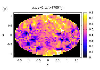
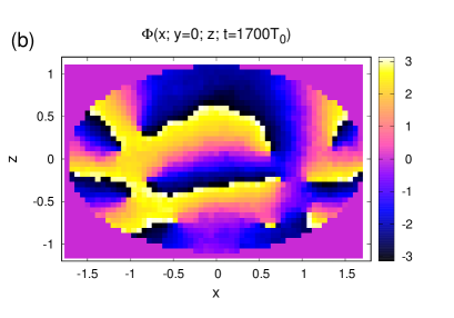
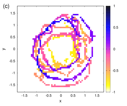
Figure 2: Vortex configuration formed at the time $t=1700T_{0}$ and the parameters $\gamma_{L}=\gamma_{C}=0.001$, $c=0.1$, and $F=0.06$: (a) energies of oscillators in the $y=0$ layer, (b) their phases, and (c) projection of vortex filaments on the $(x,y)$ plane, where the color indicates the $z$ coordinate of the sites of the lattice where $\varepsilon<0.125$. Each colored square (“pixel”) corresponds to an individual oscillator on the cubic lattice.

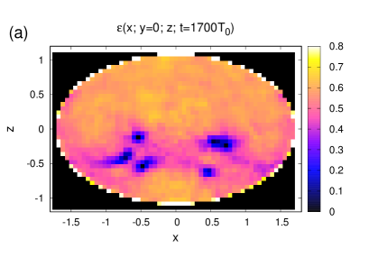
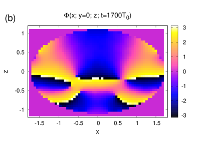
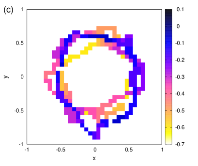
Figure 3: Vortex structure consisting of three rings that is formed at the parameters $\gamma_{L}=\gamma_{C}=0.001$, $c=0.1$, and $F=0.12$: (a) energy profile in the $y=0$ layer, (b) phases of oscillators in this layer, and (c) projection of vortex filaments on the $(x,y)$ plane.

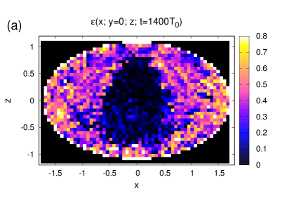
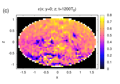
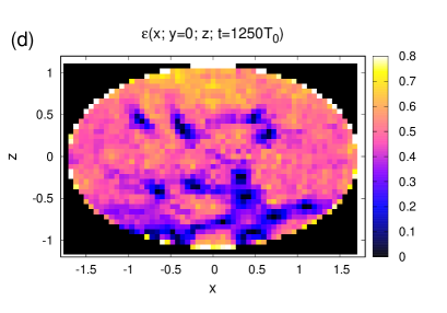
Figure 4: Energies of oscillators in the $y=0$ layer at the parameters $\gamma_{L}=\gamma_{C}=0.001$, $F=0.12$, and coupling constant $c$ = (a) 0.02, (b) 0.03, (c) 0.06, and (d) 0.12. The background at small $c$ values is not quasi-uniform. Vortices in (b) are so thin that their presence is almost unseen. These figures should be compared with Fig.3a.

The dissipative parameters $\gamma_{L}$ and $\gamma_{C}$ were for simplicity taken the same with an arbitrarily imposed condition $\gamma\geqslant 0.001$, which corresponds to the weakened requirement on the Q factor compared to the freely damping regime considered in [29].

When using Eq.(3), the detuning of the frequency of the external signal was taken $\delta=-0.1$. The sign of detuning is negative in correspondence with the negative nonlinear coefficient and negative coupling constants $c_{n,n^{\prime}}=-C_{n,n^{\prime}}/C_{0}$ (see details in [29, 30]). For brevity, the symbol $c$ will be used below for the positive quantity $C_{n,n^{\prime}}/C_{0}$.

It is important that, in contrast to systems with nonlinearity (3), where the $1\rightarrow 2$ decays certainly occur in the limit of a low energy background at $c>1/4$ and in a significantly nonlinear regime at smaller $c$ values, three-wave interactions are absent in the case of symmetric dependence (2). For this reason, increased parameters are allowed. In particular, the coupling constant was taken up to $c=2$, detuning to the extent of $\delta=-0.32$, and damping coefficient up to $\gamma=0.01$. Vortex filaments were sometimes observed even at such relatively strong damping.

A slightly perturbed quasi-uniform state was taken as the initial state. The system “forgot” it after several hundred periods. In this time (at “favorable” sets of the parameters), vortex filaments, often in the form of rings, nucleated at the boundary of the domain and then moved to the bulk, where they interacted with each other. Filaments were deformed, their symmetry was usually broken, and structures with different geometry appeared. The picture obviously was not stationary because vortices near the axis of the ellipsoid moved primarily downward, whereas vortices at the periphery moved upward. However, the characteristic statistical properties of vortices were mostly quite definite and depended strongly on the parameters.

The most typical vortex structures are shown in Figs. 2-6. Formula (3) and the parameters $h=0.06$ and $\delta=-0.1$ are common for all these figures. Other parameters are indicated in the figure captions. For a sufficiently complete visualization of an instantaneous vortex state, three pictures are usually given. The first picture shows the energy profile in the $y=0$ section of the ellipsoid. The second picture presents the quantities $\Phi_{n}=\mbox{arctg}(I_{n}/V_{n})$, which are qualitatively similar to the canonical phases $\Theta_{n}$. The third picture demonstrates the shape of vortex filaments in the $(x,y)$ projection, where the corresponding $z$ coordinate is indicated in color.

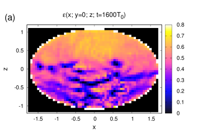
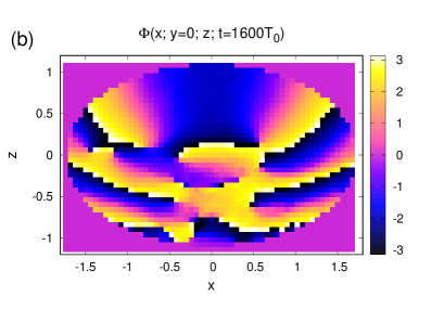
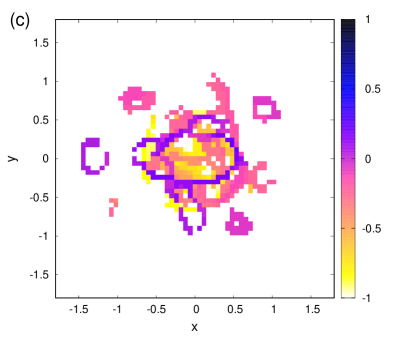
Figure 5: Vortex configuration formed at the parameters $\gamma_{L}=\gamma_{C}=0.002$, $c=0.1$, and $F=0.20$: (a) energies of oscillators in the $y=0$ layer, (b) their phases, and (c) projection of vortex filaments on the $(x,y)$ plane. Small vortex rings are seen on the periphery.

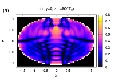
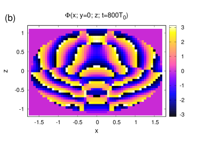
Figure 6: Coherent dissipative structure formed at the parameters $\gamma_{L}=\gamma_{C}=0.006$, $c=0.1$, and $F=0.20$: (a) energies of oscillators in the $y=0$ layer and (b) their phases. The structure consists of vortices in combination with dark solitons.

A quite developed and incompletely ordered vortex structure intensely interacting with the boundary is seen in Fig.2. Such structures appear at moderate pump amplitudes (in the case under consideration, $F=0.06$). At smaller amplitudes, the required energy background is not formed at all (e.g., at $F=0.04$; this case is not presented in the figures).

When the pump is increased to $F=0.12$, a “stricter” and “quiet” configuration consisting of three closely located vortex rings is observed, as shown in Fig.3. Rings are strongly deformed and are in the “leapfrogging” regime. It is noteworthy that similar structures consisting of four rings were observed at some other sets of parameters.

Upon increase in $F$ to 0.16 (this case is not illustrated), two or three strongly deformed mobile rings at fairly long distances from each other would be observed alternatively. At $F=0.20$ (this case is also not presented in figures), two closely located rings generally similar to rings at $F=0.12$ would be observed. The further enhancement of the pump begins to damage the background (this case is also not illustrated).

Figure 4 illustrates how the variation of the parameter $c$ affects vortex structures. It is seen in Fig.4a that overly weak links cannot transfer the energy flux sufficient to “fill” the entire domain taking into account dissipation. Only a certain pronounced layer near the boundary is filled with energy, whereas the energy in the central part is in deficit. It is noteworthy that the thickness of this layer at a given $c$ value depends primarily on the dissipative parameter $\gamma$ and slightly on the pump amplitude. A small increase in the parameter $c$ is sufficient to form a quasi-uniform background (see Fig.4b). In this case, vortices are “superdiscrete” because a significant decrease in the energy of oscillators near the axis of a vortex hardly occurs. The further enhancement of links makes cores of vortices thicker and more noticeable, as seen in Figs.4c and 4d, until the background begins to be damaged at $c\approx 0.14$ (not shown) because of the mentioned $1\rightarrow 2$ parametric processes.

Finally, Figs. 5 and 6 demonstrate the evolution of vortices with an increase in the dissipation rate. In particular, when $\gamma$ is doubled compared to Figs. 2-4, a new feature appears in dynamics: small vortex rings are produced at the periphery in the bulk of the system (see Fig.5c), which then drift toward the axis, where they join the main dissipating structure.

An increase in $\gamma$ to 0.06 fundamentally changes the entire picture, as shown in Fig.6. In this case, a stationary combined structure including dark solitons appears instead of vortex filaments. The energy background is on the whole low and far from uniform. The further enhancement of dissipation destroys the background completely.

Thus, a new regime of existence of quantized vortex filaments in weakly dissipative discrete systems has been demonstrated. Scenarios of violation of this regime under the variation of the basic parameters of the system have been revealed.

References

- (1) L. M. Pismen, Vortices in Nonlinear Fields (Clarendon, Oxford, 1999).
- (2) C. J. Pethick and H. Smith, Bose-Einstein Condensation in Dilute Gases, (Cambridge Univ. Press, Cambridge, 2002).
- (3) L. P. Pitaevskii and S. Stringari, Bose-Einstein Condensation (Oxford Univ. Press, Oxford, 2003).
- (4) P. G. Kevrekidis, D. J. Frantzeskakis, and R. Carretero-González, The Defocusing Nonlinear Schrödinger Equation: From Dark Solitons and Vortices to Vortex Rings (SIAM, Philadelphia, 2015).
- (5) B. Y. Rubinstein and L. M. Pismen, Physica D 78, 1 (1994).
- (6) A. A. Svidzinsky and A. L. Fetter, Phys. Rev. A 62, 063617 (2000).
- (7) A. L. Fetter, Rev. Mod. Phys. 81, 647 (2009).
- (8) V. P. Ruban, Phys. Rev. E 64, 036305 (2001).
- (9) J. Garcia-Ripoll and V. Perez-Garcia, Phys. Rev. A 64, 053611 (2001).
- (10) P. Rosenbusch, V. Bretin, and J. Dalibard, Phys. Rev. Lett. 89, 200403 (2002).
- (11) A. Aftalion and I. Danaila, Phys. Rev. A 68, 023603 (2003).
- (12) T.-L. Horng, S.-C. Gou, and T.-C. Lin, Phys. Rev. A 74, 041603(R) (2006).
- (13) V. A. Mironov and L. A. Smirnov, JETP Lett. 95, 549 (2012).
- (14) S. Serafini, L. Galantucci, E. Iseni, T. Bienaime, R. N. Bisset, C. F. Barenghi, F. Dalfovo, G. Lamporesi, and G. Ferrari, Phys. Rev. X 7, 021031 (2017).
- (15) C. Ticknor, W. Wang, and P. G. Kevrekidis, Phys. Rev. A 98, 033609 (2018).
- (16) V. P. Ruban, JETP Lett. 108, 605 (2018).
- (17) C. Ticknor, V. P. Ruban, and P. G. Kevrekidis, Phys. Rev. A 99, 063604 (2019).
- (18) B. A. Malomed and P. G. Kevrekidis, Phys. Rev. E 64, 026601 (2001).
- (19) P. G. Kevrekidis, B. A. Malomed, and Yu. B. Gaididei, Phys. Rev. E 66, 016609 (2002).
- (20) P. G. Kevrekidis, B. A. Malomed, D. J. Frantzeskakis, and R. Carretero-Gonzalez, Phys. Rev. Lett. 93, 080403 (2004).
- (21) P. G. Kevrekidis, B. A. Malomed, Zh. Chen, and D. J. Frantzeskakis, Phys. Rev. E 70, 056612 (2004).
- (22) D. E. Pelinovsky, P. G. Kevrekidis, and D. J. Frantzeskakis, Physica D 212, 20 (2005).
- (23) F. Lederer, G. I. Stegeman, D. N. Christodoulides, G. Assanto, M. Segev, and Ya. Silberberg, Phys. Rep. 463, 1 (2008).
- (24) J. Cuevas, G. James, P. G. Kevrekidis, and K. J. H. Law, Physica D 238, 1422 (2009).
- (25) Ya. V. Kartashov, B. A. Malomed, and L. Torner, Rev. Mod. Phys. 83, 247 (2011).
- (26) M. Lapine, I. V. Shadrivov, and Yu. S. Kivshar, Rev. Mod. Phys. 86, 1093 (2014).
- (27) J. J. Bramburger, J. Cuevas-Maraver, and P. G. Kevrekidis, Nonlinearity 33, 2159 (2020).
- (28) V. P. Ruban, Phys. Rev. E 100, 012205 (2019).
- (29) V. P. Ruban, Phys. Rev. E 102, 012204 (2020).
- (30) V. P. Ruban, JETP Lett. 111, 383 (2020).
- (31) I. V. Shadrivov, A. A. Zharov, N. A. Zharova, and Yu. S. Kivshar, Photonics Nanostruct. Fundam. Appl. 4, 69 (2006).
- (32) N. N. Rosanov, N. V. Vysotina, A. N. Shatsev, I. V. Shadrivov, and Yu. S. Kivshar, JETP Lett. 93, 743 (2011).
- (33) R. Hirota and K. Suzuki, J. Phys. Soc. Jpn. 28, 1366 (1970).
- (34) R. Hirota and K. Suzuki, Proc. IEEE 61, 1483 (1973).
- (35) A. C. Hicks, A. K. Common, and M. I. Sobhy, Physica D 95, 167 (1996).
- (36) A. C. Singer and A. V. Oppenheim, Int. J. Bifurc. Chaos 9, 571 (1999).
- (37) D. Cai, N. Gronbech-Jensen, A.R. Bishop, A.T. Findikoglu, and D. Reagor, Physica D 123, 291 (1998).
- (38) T. Kofane, B. Michaux, and M. Remoissenet, J. Phys. C: Solid State Phys. 21, 1395 (1988).
- (39) P. Marquie, J. M. Bilbault, and M. Remoissenet, Phys. Rev. E 49, 828 (1994).
- (40) P. Marquie, J. M. Bilbault, and M. Remoissenet, Phys. Rev. E 51, 6127 (1995).
- (41) V. A. Makarov, E. del Rio, W. Ebeling, and M. G. Velarde, Phys. Rev. E 64, 036601 (2001).
- (42) D. Yemele, P. Marquie, and J. M. Bilbault, Phys. Rev. E 68, 016605 (2003).
- (43) L. Q. English, F. Palmero, A. J. Sievers, P. G. Kevrekidis, and D. H. Barnak, Phys. Rev. E 81, 046605 (2010).
- (44) F. Palmero, L. Q. English, J. Cuevas, R. Carretero-Gonzalez, and P. G. Kevrekidis, Phys. Rev. E 84, 026605 (2011).
- (45) L. Q. English, F. Palmero, J. F. Stormes, J. Cuevas, R. Carretero-Gonzalez, and P. G. Kevrekidis, Phys. Rev. E 88, 022912 (2013).
- (46) F. Palmero, L. Q. English, X.-L. Chen, W. Li, J. Cuevas-Maraver, and P. G. Kevrekidis, Phys. Rev. E 99, 032206 (2019).
- (47) C. J. G. Meyers, C. R. Freeze, S. Stemmer, and R. A. York, Appl. Phys. Lett. 109, 112902 (2016).
- (48) Y. Shen, P. G. Kevrekidis, G. P. Veldes, D. J. Frantzeskakis, D. DiMarzio, X. Lan, and V. Radisic, Phys. Rev. E 95, 032223 (2017).
- (49) A. P. Slobozhanyuk, P. V. Kapitanova, I. V. Shadrivov, P. A. Belov, and Yu. S. Kivshar, JETP Lett. 95, 613 (2012).