Critical properties of the Susceptible-Exposed-Infected model with correlated temporal disorder

Abstract

In this paper we study the critical properties of the non-equilibrium phase transition of the Susceptible-Exposed-Infected model under the effects of long-range correlated time-varying environmental noise on the Bethe lattice. We show that temporal noise is perturbatively relevant changing the universality class from the (mean-field) dynamical percolation to the exotic infinite-noise universality class of the contact process model. Our analytical results are based on a mapping to the one-dimensional fractional Brownian motion with an absorbing wall and is confirmed by Monte Carlo simulations. Unlike the contact process, our theory also predicts that it is quite difficult to observe the associated active temporal Griffiths phase in the long-time limit. Finally, we also show an equivalence between the infinite-noise and the compact directed percolation universality classes by relating the SEI model in the presence of temporal disorder to the Domany-Kinzel cellular automaton in the limit of compact clusters.

I Introduction

Absorbing phase transitions are non-equilibrium phase transitions separating an inactive phase without fluctuations (absorbing) from an active (fluctuating) one. This type of phase transition is observed in many models for a great variety of phenomena such as epidemic spreading (Harris, 1974a; Grassberger, 1983), interface growth (Barabasi and Stanley, 1995), catalytic chemical reactions (Ziff et al., 1986), turbulent crystal liquids (Takeuchi et al., 2007, 2009), periodically driven suspensions (Corte et al., 2008; Franceschini et al., 2011), superconducting vortices (Okuma et al., 2011) and bacteria colony biofilms (Korolev and Nelson, 2011; Korolev et al., 2011). (See, e.g., Refs. Marro and Dickman, 1999; Hinrichsen, 2000; Odor, 2004; Henkel et al., 2008 for reviews). Recently, absorbing state phase transitions have also been observed in open driven many-body quantum systems (Gutiérrez et al., 2017).

An important and thoroughly studied universality class of absorbing phase transitions is the “ubiquitous” directed percolation (DP) universality class (Grassberger and de la Torre, 1979; Janssen, 1981; Grassberger, 1982; Marro and Dickman, 1999; Hinrichsen, 2000; Odor, 2004; Henkel et al., 2008). For many years it has evaded experimental confirmation (Takeuchi et al., 2007; Lemoult et al., 2016; Sano and Tamai, 2016; Kohl et al., 2016). Earlier, it was thought that one possible reason was due to quenched disorder as the DP universality class is perturbatively unstable against it for $d<4$ (Harris, 1974b; Kinzel, 1985; Noest, 1986). It was then determined that quenched disorder in the contact process (Harris, 1974a) (a prototypical model exhibiting a transition in the DP universality class) induces a rich physical scenario with a universal (disorder-independent) infinite-randomness critical point governing the critical properties, in addition to off-critical Griffiths singularities in the inactive phase (Hooyberghs et al., 2003, 2004; Vojta and Dickison, 2005; Hoyos, 2008; de Oliveira and Ferreira, 2008; Vojta et al., 2009; Vojta, 2012; Vojta and Hoyos, 2014; Vojta et al., 2014; Wada and de Oliveira, 2017). For a review on the exotic properties of the infinite-randomness universality class and the corresponding Griffiths phase, see, e.g., Ref. Vojta, 2006. Despite of this theoretical achievement, an experimental confirmation of this exotic critical behavior is still lacking in non-equilibrium phase transitions.

The effects of time-dependent global fluctuations (temporal disorder) has also attracted attention (Leigh Jr., 1981; Kinzel, 1985; Jensen, 1996, 2005; Kamenev et al., 2008; Ovaskainen and Meerson, 2010; Vazquez et al., 2011; Vojta and Hoyos, 2015; Barghathi et al., 2016; de Oliveira and Fiore, 2016; Fiore et al., 2018). Like its spatial counterpart, it is a relevant perturbation for the DP critical behavior (Kinzel, 1985), except that it is relevant in all dimensions. The physical behavior is equally rich as well. An infinite-noise critical point governs the transition in all dimensions (Vojta and Hoyos, 2015; Barghathi et al., 2016) (implying ever increasing relative density fluctuations) and an associated active Griffiths phase also exists (Vazquez et al., 2011). In $d=\infty,$ the infinite-noise critical point is akin to the infinite-randomness critical point with the roles of time and space exchanged. It turns out that the relative density fluctuations increase unbounded $\sim t^{1/2}$. For finite $d$, the infinite-noise critical point is qualitatively different, and is akin to the disordered Kosterlitz-Thouless critical point in dissipative quantum rotors (Vojta et al., 2011) and in the quantum Ising model with long-range couplings (Juhász et al., 2014). In addition, the relative density fluctuations increase only $\sim\ln t$. Later on, the effects of correlated noise was also investigated in the $d=\infty$ limit (Wada et al., 2018). It was observed an increase (decrease) of the critical and off-critical fluctuations when the correlations are positive (negative).

Given this “ubiquitous” infinite-noise criticality, it is desirable to know whether a similar scenario also happens in other non-equilibrium phase transition which are not in the DP universality class. We then study the Susceptible-Exposed-Infected (SEI) model which exhibits a non-equilibrium phase transition into an absorbing state in the dynamical percolation universality class (Tomé and de Oliveira, 2011; Wada et al., 2015). Considering the model on the Bethe lattice, we could solve the effects of correlated temporal disorder by mapping the problem onto a fractional Brownian motion with an absorbing wall (fBMAW). We show that this model exhibits the same infinite-noise critical behavior as in the ($d=\infty$) contact process, but very distinct off-critical Griffiths phase. In addition, our analytical results are confirmed by Monte Carlo simulations. Finally, we also uncover an equivalence between the infinite-noise and the compact directed percolation universality classes. This is done by a one-to-one correspondence between the critical dynamics of the SEI model and of the Domany-Kinzel cellular automaton (Domany and Kinzel, 1984) in the limit of compact clusters . Therefore, we show that the notion of infinite-noise criticality is more common than previously thought.

This paper is organized as follows. We introduce the SEI model with temporal disorder and the mapping onto fBMAW in Sec. II. In Sec. III we develop our theory and derive the critical behavior of key observable in order to characterize the universality class. The Monte Carlo simulations confirming our theory are presented in Sec. IV. Finally, we uncover the equivalence between the compact directed percolation and the infinite-noise universality classes in Sec. V, and conclude in Sec. VI with final remarks.

II Susceptible-Exposed-Infected model

II.1 Definition

The Susceptible-Exposed-Infected (SEI) model (Tomé and de Oliveira, 2011) was introduced to describe the spreading of a certain disease on a susceptible population. In this model individuals are lattice sites and the interactions occur only between infected (I) and susceptible (S) nearest neighbor individuals. When an interaction takes place, the S individual either becomes exposed (E) or infected (I) with rates $\mu$ and $\lambda$ respectively. We emphasize that neither E or I individuals are allowed to change their state, and E individuals do not spread the disease. Figure 1 shows the possible reactions.

Figure 1: Reactions of the susceptible-exposed-infected (SEI) model. In the presence of an infected nearest neighbor, susceptible individuals becomes either exposed or infected with rates $\mu$ and $\lambda$, respectively.

Therefore, the system is active whenever the number $n_{IS}$ of susceptible-infected pairs (active bonds) is nonzero. In a finite regular lattice, the SEI model will eventually reach an absorbing state characterized by a cluster of I sites surrounded by $E$ ones. Notice that the model admits an infinite number of absorbing states.

We now explain the simulation algorithm according to the Gillespie method (Gillespie, 1976). We maintain a list of the $n_{IS}$ active bonds and proceed as follows: (i) increase time by $1/(n_{IS}r)$, where $r$ is a uniformly distributed random number in the interval $]0,1[$; (ii) select, at random and with equal probability, one active bond in the list; (iii) the S site of the selected bond either becomes E with probability $q=\mu/(\mu+\lambda)$, or becomes I with probability $p=1-q$; (iv) update the list of active bonds; (v) return to (i) until there are no active bonds.

Interestingly, the above algorithm reveals a direct connection between the SEI model and the isotropic site percolation problem. Consider, for instance, a lattice in which all sites are initially in state S except for one which is in the I state. At the end of the simulation, the Gillespie algorithm will have generated a cluster of I sites surrounded by E ones where each of them were asked just once whether they are at the E (vacant) or I (occupied) state, just like in the isotropic percolation problem (Stauffer and Aharony, 1994). (The remaining S sites which did not participate in the simulation are not important here.) Therefore, the SEI model exhibits a phase transition in the dynamical percolation universality class. For $p<p_{c}$ (the isotropic percolation threshold), the generated I cluster is finite (inactive phase), whereas an infinite one is possible for $p>p_{c}$ (active phase). Furthermore, the static critical exponents such as $\beta$ and $\nu_{\perp}$ are the same as those of isotropic percolation.

II.2 Solution on the Bethe lattice

We now review the solution of the SEI model on a infinite Bethe lattice (Tomé and de Oliveira, 2011) restricting ourselves to the initial condition of a single cluster of I sites in a lattice filled of S sites. In this case, any arbitrary cluster configuration containing $n_{I}$ infected sites will have a number of individuals on its perimeter that only depends on $n_{I}$. In other words, although it is possible to rearrange the connected cluster of I individuals in many different ways, the number of sites on the perimeter depends only on $n_{I}$ regardless of the particular cluster rearrangement. In fact, the number exposed individuals $n_{E}$, $n_{IS}$ and $n_{I}$ are related via

$$n_{IS}+n_{E}=(z-2)n_{I}+2,$$ (1)

where $z$ is the coordination number. Notice that the left hand side is the number of sites at the perimeter of the cluster of I individuals.

The time evolution of the average number of infected, exposed and active bonds, $N_{I}=\langle n_{I}\rangle$, $N_{E}=\langle n_{E}\rangle$ and $N_{IS}=\langle n_{IS}\rangle$, where $\langle\ldots\rangle$ is the average over the stochastic noise, can be obtained from the following differential equations:

$$\frac{\text{d}}{\text{d}t}N_{I} =\lambda N_{IS},$$ (2)

$$\frac{\text{d}}{\text{d}t}N_{E} =\mu N_{IS},$$ (3)

$$\frac{\text{d}}{\text{d}t}N_{IS} =-\left(\mu+\lambda\right)N_{IS}+(z-1)\lambda N_{IS},$$ (4)

where we have redefined $\lambda\rightarrow z\lambda$ and $\mu\rightarrow\mu z$ for convenience. These equations can be solved exactly yielding to

$$N_{I} =\frac{\mu_{c}N_{IS}^{0}}{(z-2)\left(\mu_{c}-\mu\right)}\left(e^{(\mu_{c}-\mu)t}-1\right)+N_{I}^{0},$$ (5)

$$N_{E} =\frac{\mu N_{IS}^{0}}{\mu_{c}-\mu}\left(e^{(\mu_{c}-\mu)t}-1\right)+N_{E}^{0},$$ (6)

$$N_{IS} =N_{IS}^{0}e^{(\mu_{c}-\mu)t},$$ (7)

with

$$\mu_{c}=\left(z-2\right)\lambda.$$ (8)

Note that Eq. (1) is satisfied provided that $N_{IS}^{0}+N_{E}^{0}=(z-2)N_{I}^{0}+2$.

There are three distinct behaviors. The active phase ($\mu<\mu_{c}$) is characterized by a diverging $N_{IS}$ as $t\rightarrow\infty$ whereas in the inactive phase ($\mu<\mu_{c}$) $N_{IS}\rightarrow 0$ as $t\rightarrow\infty$. The critical point happens for $\mu=\mu_{c}$ where $N_{IS}$ is constant in time, and $N_{I}$ and $N_{E}$ grow only linearly with $t$.

II.3 Temporal disorder and the mapping onto a fractional Brownian motion with an absorbing wall

We are interested in the situation where the system is under the influence of environmental noise. Following Ref. Vojta and Hoyos, 2015, we introduce temporal disorder by allowing the rates $\mu$ and $\lambda$ to change randomly after remaining constant during a time interval of size $\Delta t_{n}>0$. Thus, the rates at the $n$th time interval are $\mu_{n}=\mu+\Delta\mu_{n}$ and $\lambda_{n}=\lambda+\Delta\lambda_{n}$ with $\lambda$ and $\mu$ being constants and $\Delta\mu_{n}$ and $\Delta\lambda_{n}$ being zero-average noises.

Given the sequence $\left\{\lambda_{n},\mu_{n}\right\}$, the complete time evolution of $N_{IS},$ $N_{E}$ and $N_{I}$ is thus obtained by patching the solutions (5), (6) and (7) in each time interval. The solution for $N_{IS}$ reads

$$N_{IS}^{(n+1)} =N_{IS}^{(n)}e^{\left(\mu_{c,n}-\mu_{n}\right)\Delta t_{n}},$$ (9)

where $N_{IS}^{(n)}$ is the stochastic average of $n_{IS}$ at the beginning of the $n$th time interval and $\mu_{c,n}\equiv(z-2)\lambda_{n}$. It is convenient to recast Eq. (9) in terms of $x_{n}=\ln(1+N_{IS}^{(n)})$: $x_{n+1}=\ln\left(1+\left(e^{x_{n}}-1\right)e^{\left(\mu_{c,n}-\mu_{n}\right)\Delta t_{n}}\right)$. In the $x_{n}\gg 1$ limit, the time evolution of $x$ then becomes a simple random walk

$$x_{n+1}=x_{n}+\zeta_{n}$$ (10)

with an absorbing wall at $x=0$ (ensuring $N_{IS}\geq 0$) and noise

$$\zeta_{n}=\left(\mu_{c,n}-\mu_{n}\right)\Delta t_{n}=\left((z-2)\lambda_{n}-\mu_{n}\right)\Delta t_{n}.$$ (11)

The mean bias is thus

$$v=\left[\frac{\zeta_{n}}{\Delta t_{n}}\right]=\mu_{c}-\mu,$$ (12)

with $\mu_{c}=\left[\mu_{c,n}\right]=\left(z-2\right)\lambda$ as in the clean case Eq. (8). Here, $\left[\cdots\right]$ denotes the average over the temporal disorder. Clearly, $v>0$ means that $N_{IS}$ typically increases in time and thus the system is in the active phase. On the other hand, the inactive phase happens for $v<0$ since the system will eventually reach the absorbing state. Finally, the transition takes place for $v=0$.

In order to obtain a complete description of the critical behavior, we will need the noise correlation function

$$G(i,j)=[\zeta_{i}\zeta_{j}]-[\zeta_{i}][\zeta_{j}].$$ (13)

In this work, we will assume a fractional Gaussian noise (Qian, 2003)

$$G(i,j)=G(\tau)=\frac{\sigma^{2}}{2}(|\tau+1|^{2-\gamma}-2|\tau|^{2-\gamma}+|\tau-1|^{2-\gamma}),$$ (14)

which decays $\sim(1-\gamma)\tau^{-\gamma}$ for large $\tau=|i-j|$. Here, the correlation exponent $\gamma$ takes any value in the interval $]0,2[$ and is related to the Hurst exponent $H$ through $2H=2-\gamma$. This implies that the fractional Gaussian noise is positively correlated for $\gamma<1$, negatively correlated for $\gamma>1$, and uncorrelated for $\gamma=1$. Finally, $\sigma^{2}$ is the variance of the noise $\zeta$.

We end this section by summarizing our results so far. In the large $N_{IS}$ limit, the SEI model with the correlated temporal disorder (14) can be mapped onto a fractional Brownian motion with an absorbing wall (fBMAW) at $x=0$ with each step of the walker $n\rightarrow n+1$ corresponding to the time increasing $t\rightarrow t+\Delta t_{n}$ in the SEI model. We will make use of this fact to study the system behavior near the transition. We anticipate that our results are accurate even though the approximation fails near the absorbing wall. The reason for such, as in the contact process (Vojta and Hoyos, 2015; Wada and Vojta, 2018) and related models (Fiore et al., 2018), is that details of the wall are irrelevant for the singular critical behavior.

III Theory

III.1 Generalized Harris criterion

Before developing the theory, let us first discuss whether the clean critical behavior is perturbatively unstable against correlated temporal disorder. Following Harris (Harris, 1974b), we need to study the distribution $Q(\psi)$ of the coarse-grained distances from criticality as the critical point is approached. Such probability distribution is obtained by averaging $\zeta_{n}$ in Eq. (11) over a time window of order of the clean correlation time $\xi_{t}$. For $\xi_{t}\rightarrow\infty$, $Q(\psi)$ is known since $\zeta_{n}$ is a fractional Gaussian noise (Qian, 2003). It is simply a Gaussian with the mean $\bar{\psi}=[\zeta_{n}]=\zeta$ and variance $\sigma_{\psi}^{2}=\xi_{t}^{-\gamma}$, where $\gamma$ is the correlation exponent in Eq. (14). A necessary condition for the stability of clean critical theory is that $\sigma_{\psi}/\left|\text{$\bar{\psi}$}\right|\rightarrow 0$ as $\bar{\psi}=\zeta\rightarrow 0$. Since $\zeta\sim\xi_{t}^{-1/\nu_{\parallel}^{(c)}}$, where $\nu_{\parallel}^{(c)}$ is the correlation time exponent of the clean theory, then we conclude that the system is unstable against fractional Gaussian correlated temporal disorder if

$$\gamma\nu_{\parallel}^{(c)}<2.$$ (15)

As the SEI model belongs to the dynamical percolation universality class, then $\nu_{\parallel}^{(c)}=1$ for $d\geq 6$ (Henkel et al., 2008), therefore disorder is relevant for all $\gamma$ in the Bethe lattice. For $d<6$ correlated disorder is also a relevant perturbation for some values of $\gamma$.

We end this section by emphasizing that the effects of correlated disorder can be studied in a completely generic scenario. According to Ref. Vojta and Dickman, 2016, the clean critical behavior is unstable against weak temporal disorder if

$$\lim_{\xi_{t}\rightarrow\infty}\xi_{t}^{2/\nu_{\parallel}^{(c)}-1}\int_{0}^{\xi_{t}}\text{d}tG(t)\rightarrow\infty,$$ (16)

where $G(t)$ is the noise correlation function (13). Inserting (14) onto (16), the criterion (15) is recovered. However, the integral (16) yields two terms for a more generic power-law correlation such as $G(t)\propto\left(1+\left|t\right|\right)^{-\gamma}$: one proportional to $\xi_{t}^{1-\gamma}$ and the other is a constant. (For the fractional Gaussian noise the constant term is zero, i.e., the white noise component is vanishing.) This means that a white noise is present in the latter case but not in the fractional Gaussian noise. For $\gamma<1$ the first term dominates and the criterion follows as in Eq. (15). For $\gamma>1$, on the other hand, the constant term dominates in the latter case and the criterion changes to $\nu_{\parallel}^{(c)}<2$. Therefore the system should be unstable against the generic power-law correlated noise $G\propto(1+\left|t\right|)^{-\gamma}$ if $\text{min}\{1,\gamma\}\nu_{\parallel}^{(c)}<2$.

III.2 Critical properties

As discussed in Sec. II.3 when mapping the SEI model onto a fBMAW, we expect activity to (i) vanish exponentially fast if the bias (12) is towards the absorbing wall, (ii) to vanish slowly if the bias is zero, and (iii) to persist indefinitely if the walkers are driven away from the wall. Therefore $v<0$ is the inactive phase, $v=0$ is the critical point, and $v>0$ is the active phase.

We start our analysis by identifying the order parameter. Since the clean critical theory of the SEI model is in the dynamical percolation universality class, the order parameter is the percolation probability ${\cal P}$ which is linearly proportional to the survival probability, i.e., the probability that the system has never reached $n_{IS}=0$. In the fBMAW framework, the survival probability is the persistence probability which, for zero bias velocity and large number of steps $n\gg 1$, is known to decay as (Krug et al., 1997; Zoia et al., 2009; Wiese et al., 2011a)

$${\cal P}\sim t^{-\delta},$$ (17)

with $\delta=\gamma/2$ and $t=\Delta t_{1}+\dots+\Delta t_{n}\approx n\left[\Delta t_{n}\right]$.

We now turn our attention to $N_{IS}$. Since $\left[N_{IS}\right]\sim\left[e^{x}\right]$, the leading behavior of $N_{IS}$ is given by the large-$x$ behavior of the fBMAW. According to Ref. (Wiese et al., 2011b), the probability density of the fBMAW after $n\gg 1$ steps decays as

$$P_{\text{tail},n}\left(x\right)\sim\exp\left[-x^{2}/(2\sigma^{2}n^{2-\gamma})\right]$$ (18)

for large $x$ and up to a subleading power-law correction. Thus,

$$[N_{IS}]\sim\int_{0}^{\infty}e^{x}\exp\left[-x^{2}/\left(2\sigma^{2}n^{2-\gamma}\right)\right]\text{d}x\sim e^{At^{\theta}},$$ (19)

with $\theta=2-\gamma$ and $A$ being a constant, i.e., $\left[N_{IS}\right]$ grows exponentially at the critical point. Notice that $\left[N_{IS}\right]$ grows faster than $e^{vt}$ if $\gamma<1$ which is physically impossible since $\left[N_{IS}\right]$ can not grow faster than the growth in the clean active phase (7). This accelerated growth happens due to $\left[N_{IS}\right]$ been dominated by the arbitrarily high noise values generated by correlated Gaussian distribution. In a real situation the noise is bounded $\left|\xi_{n}\right|<\xi_{\text{max}}$ implying that $N_{IS}$ can be at best proportional to $e^{\xi_{\text{max}}n}$. Setting $\xi_{\text{max}}n$ as the upper limit of the integral (19), we find that $\theta=\min\{1,2-\gamma\}.$

We now show that the arithmetic $\left[N_{IS}\right]\sim\left[e^{x}\right]$ and the geometric $N_{IS}^{\text{typ}}\sim e^{[x]}$ averages are quite different. Starting at $t=0$ from $x_{0}=\ln(1+N_{IS}^{0})$ the walkers perform an unbounded fBM until they reach the absorbing wall. The large-$x$ behavior of the surviving walkers are thus dictated by (18) and hence $\left[x\right]_{\text{surv}}\sim\int_{0}^{\infty}\text{d}xxP_{\text{tail},n}\left(x\right)\sim t^{1-\gamma/2}$. As expected, it scales as the width of $P_{\text{tail},n}$. Finally, taking into consideration the surviving probability, we find that

$$\ln\left(1+N_{IS}^{\text{typ}}\right)\sim\left[x\right]\sim t^{1-\gamma/2}{\cal P}\sim t^{\alpha},$$ (20)

with $\alpha=1-\gamma$. Interestingly, notice that $x$ grows if the correlations are positive $\gamma<1$, vanishes if the correlation are negative $\gamma>1$, and remains constant in the uncorrelated case $\gamma=1$. As anticipated, the arithmetic and geometric averages behave quite different at criticality as can be quantified via $\ln[N_{IS}]/\ln N_{IS}^{\text{typ}}\sim t$. Such strong difference is a hallmark of the infinite-noise criticality.

III.3 Off-critical properties

After analyzing some critical properties of the system where exponents $\delta$, $\theta$ and $\alpha$ were founded, we now turn attention to the off-critical behavior. We start with the correlation time $\xi_{t}$. Without resorting to the time correlation function, $\xi_{t}$ can be evaluated as the time at which the average position of the surviving walkers $\left[x\right]_{\text{surv}}$ crosses over from the critical to the off-critical average position. As we have seen, at criticality $\left[x\right]_{\text{surv}}\sim t^{(2-\gamma)/2}$. In the active phase, the walkers are subject to a bias velocity $v>0$ and therefore the average position grows ballistically $\left[x\right]_{\text{surv}}\propto vt$ for $t\gg 1$. The crossover (correlation) time between the critical and off-critical regimes is thus

$$\xi_{t}\sim|v|^{-\nu_{\parallel}},$$ (21)

with $\nu_{\parallel}=2/\gamma$, which saturates the generalized Harris criterion (15).

What about the order parameter? It is proportional to the stationary survival probability ${\cal P}_{\text{st}}$ which can be estimated as the critical ${\cal P}$ in (17) at the crossover (correlation) time $\xi_{t}$ in (21). Therefore,

$${\cal P}_{\text{st}}\sim v^{\beta},$$ (22)

where $\beta=\delta\nu_{\parallel}=1$ is a $\gamma$-independent critical exponent.

Can we determine the relation between the correlation length $\xi$ and the correlation time $\xi_{t}$? On the Bethe lattice, the notion of length is not clear. Nevertheless, we can define a compact cluster of size $\xi$ containing $N_{IS}\sim\xi^{d}$ active bonds. In the active phase, this cluster grows ballistically in time as $\ln N_{IS}\sim v\xi_{t}$. Therefore, together with (21) we find that

$$\ln\xi\sim\xi_{t}^{\psi},$$ (23)

with “tunneling” exponent $\psi=1-\nu_{\parallel}^{-1}=1-\gamma/2=H$, which equals the Hurst exponent. This activated dynamic scaling relation between length and time scales is another hallmark of the infinite-noise critical behavior.

Let us remark that the exponents $\theta$, $\alpha$, $\delta$, $\nu_{\parallel}$ and $\psi$ are $\gamma$-dependent. If one uses another noise correlation function instead of (14) such as $G\propto(1+\left|t\right|)^{-\gamma}$, then our results hold for $\gamma\leq 1$ (positive correlations), while for $\gamma>1$ these exponents remain the same as for the uncorrelated case $\gamma=1$. We end this section by comparing the critical exponents here reported to those of the contact process and its generalizations. The exponents $\delta$, $\nu_{\parallel}$, $\beta$, and $\psi$ [respectively in Eqs. (17), (21), (22) and (23)], were also computed in those models (Vojta and Hoyos, 2015; Fiore et al., 2018; Wada et al., 2018) and are numerically equal. Thus, the critical behavior of SEI model here studied is in the same infinite-noise universality class of the contact process in $d=\infty$.

III.4 Absence of the temporal Griffiths phase

In the contact process, the active temporal Griffiths phase (Vazquez et al., 2011) is caused by rare sequences of large time intervals in which the system is temporarily in the inactive phase while the system is actually in the active one. As a consequence, these rare time intervals causes strong density fluctuations near criticality. Can we observe an analogous effect in the SEI model?

Let us analyze the probability for a walker to get absorbed in the active phase $v>0$. In this case, the distribution of the walker position is a Gaussian centered at $\left\langle x\right\rangle\sim vt$ and width $\sqrt{\left\langle x^{2}\right\rangle-\left\langle x\right\rangle^{2}}\sim t^{\psi}$, with $\psi=1-\gamma/2$. Since $\psi<1$, the probability for a particle to get absorbed goes to zero in the long-time limit. As a consequence, the relative density fluctuations will vanish $\sim t^{\psi-1}$ with a prefactor that is inversely proportional to $x_{0}$. In fact, we could not observe the active temporal Griffiths phase in our simulations for $x_{0}\gtrsim 5$. A similar argument can be applied to the inactive temporal Griffiths phase.

IV Monte-Carlo simulations

In this section we report our Monte Carlo simulations on the SEI model with correlated temporal disorder and compare the numerical results with the analytical theory.

IV.1 The algorithm, the random variables and the averages

In our simulations we start with a single cluster of $n_{I}^{0}$ infected individuals on a lattice full of susceptible ones ($n_{E}^{0}=0$, and thus $n_{IS}^{0}=\left(z-2\right)n_{I}^{0}+2$). As explained in Sec. II.1, activity occurs at the border of this cluster and the lattice is irrelevant for the simulations. Therefore, only the number of $n_{IS}$ pairs is necessary for the simulation. Let $r_{1}$ and $r_{2}$ be uniformly distributed random numbers in the interval $]0,1[$, and $p_{n}=\lambda_{n}/(\lambda_{n}+\mu_{n})$. Our algorithm then reads:

1. increase time $t$ by $1/(n_{IS}r_{1})$.

2. generate new values of $\mu_{n}$ and $\lambda_{n}$ if the integer part of the discrete time $n=t/\Delta t$ has increased by one unity.

3. if $r_{2}<p_{n}$, an S site becomes $I$. This means that we need to increase the number of $IS$ pairs by $z-2$. On the other hand, if $r_{2}\geq p_{n}$, the $S$ site becomes $E$ which decreases the number of IS pairs by one.

4. return to (i) until $n_{IS}=0$.

However, despite this algorithm being of easy implementation and allow us to simulate system sizes as large as the computer precision, it is very slow for large $n_{IS}$ since the time increasing is, on average, only $\sim 1/n_{IS}$ at each iteration. In other words, the simulation time increases exponentially with $n_{IS}$.

In order to optimize the SEI simulations, we will use a combination of the above mentioned algorithm and the analytical result (9). First, we introduce a cutoff $N_{IS}^{\text{cutoff}}=10^{3}$. When $n_{IS}<N_{IS}^{\text{cutoff}}$, $n_{IS}$ is small and we can use the SEI Monte Carlo algorithm above described. If $n_{IS}>N_{IS}^{\text{cutoff}}$, $n_{IS}$ is very large and we expect the stochastic noise to average out. Therefore, $n_{IS}$ should be well described by its stochastic average $N_{IS}$.

Having described the SEI simulation algorithm, we now explain the generation of power-law correlated noise. Following Refs. Wada et al., 2018; Wada and Vojta, 2018; Wada et al., 2019, we employ the Fourier filtering method (Makse et al., 1996) to generate Gaussian correlated noise following the correlation function (14). We first generate a set $\nu_{n}$ of zero average Gaussian uncorrelated numbers of variance $1$. The Gaussian power-law correlated random numbers $\zeta_{n}$ are given by the inverse Fourier transform of

$$\tilde{\zeta}_{\omega}=[\tilde{G}_{\text{fBM}}(\omega)]^{1/2}\tilde{\nu}_{\omega},$$ (24)

where $\tilde{\nu}_{\omega}$ and $\tilde{G}_{\text{fBM}}$ are the Fourier transform of $\nu_{n}$ and of the correlation function (14), respectively. A noise of variance $\sigma^{2}$ can be obtained by multiplying $\zeta{}_{n}$ by $\sigma$.

In the following simulations we fix $\lambda_{n}=\lambda$ and $\mu_{n}=\mu+\Delta\mu_{n}$ is the source of temporal disorder, i.e., $\Delta\mu_{n}$ is a zero-mean Gaussian noise with variance $\sigma^{2}$. To control the distance to the critical point $v$ (12), we choose $\mu=128$ (sufficiently large ensuring that $\mu_{n}>0$ in our simulations) and vary only $\lambda$. All simulations use the coordination number $z=4$ (so the critical point $v=0$ happens for $\lambda=64$) and run up to $t=10^{8}$. Furthermore, for convenience, time will always be renormalized by a factor of $1/(\mu+\lambda)$. Therefore, for a small time window $\delta t$, $n_{IS}\delta t$ processes take place on average.

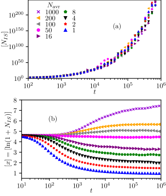
Figure 2: Simulations of the SEI model with uncorrelated temporal disorder ($\gamma=1$) at the critical point $v=(z-2)\lambda-\mu=0$. Here $\lambda=64$, $\mu=128$, $\sigma=8$, $\Delta t=16,$ the initial cluster has size $N_{IS}^{0}=10^{2}$, and the data is averaged over ${\cal N}=10^{5}$ temporal disorder configurations and over $N_{\text{avr}}$ realizations of the stochastic noise. In panel (a) the uncertainties are of the order of the dispersion of the data and in panel (b) of the order of the symbol size.

Finally, let us discuss about the combined stochastic and external noise averages $\left[\left\langle{\cal A}\right\rangle\right]$ of a certain observable ${\cal A}$. The estimates of the stochastic $\left\langle{\cal A}\right\rangle$ and the external noise $\left[{\cal A}\right]$ averages are taken over $N_{\text{avr}}$ stochastic noise and ${\cal N}$ temporal disorder realizations, respectively. Interestingly, we find in our simulations that near criticality $N_{\text{avr}}$ can be as low as $1$ and ${\cal N}\gg 1$. This is the first confirmation of our theory. The infinite noise critical point is characterized by long incursions of the system in either of the phases around the transition point yielding to ever larger fluctuations. In other words, effectively the system is never under the clean critical point influence, but fluctuating around and far from it. This is seen in Fig. 2. In panel (a), $\left[\left\langle n_{IS}\right\rangle\right]$ is shown as a function of time for the case of uncorrelated disorder $\gamma=1$ and at criticality $\mu=\mu_{c}$. We have averaged over ${\cal N}=10^{5}$ temporal disorder configurations and over different values of stochastic noise $N_{\text{avr}}$ ranging from as low as $N_{\text{avr}}=1$ up to $N_{\text{avr}}=10^{3}$. Clearly, $\left[N_{IS}\right]$ is barely sensitive to $N_{\text{avr}}$ within the temporal disorder statistical error. Likewise, we plot $\left[x\right]=\left[\ln\left(1+N_{IS}\right)\right]$ in panel (b) as a function of time. The effects of different values of $N_{\text{avr}}$ is only quantitative higher since $\left[x\right]\rightarrow\text{const}$ as $t\rightarrow\infty$. The reason for this stronger effect is because the typical average is not dominated by tail of the probability distribution as is $\left[N_{IS}\right]$. Since neither $\left[\left\langle n_{IS}\right\rangle\right]$ nor $\left[\ln\left\langle 1+n_{IS}\right\rangle\right]$. are qualitatively affected by $N_{\text{avr}}$ we will take $N_{\text{avr}}=1$ from now on.

IV.2 Critical properties

Having discussed the details of our simulations, we now report on our numerical results.

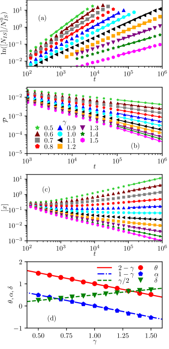
Figure 3: Simulations of the SEI model with power-law correlated temporal disorder at the critical point. In all panels the uncertainties are of the order of the symbol size, and the solid lines are power-law fits. (a) $\ln([N_{IS}]/N_{IS}^{0}$) vs. $t$. for many values of the correlation exponent $\gamma$ [see Eq. (14)]. These simulations used the parameters $\sigma=1$, $\Delta t=4$ and initial condition $N_{IS}^{0}=4$. (b,c) the survival probability ${\cal P}$ and the average position $[x]=\ln(1+N_{IS})$ as a function of time for $\sigma=8$, $\Delta t=16$ and initial condition $N_{IS}^{0}=4$. (d) The critical exponents extracted by fitting power laws to the data according to the equations (19), (17) and (20), for $N_{IS}$, ${\cal P}$ and $x$, respectively. All simulations averages over $10^{7}$ disorder configurations.

Figure 3(a) shows our simulations for $\ln([N_{IS}]/N_{IS}^{0})$ at the critical point for many values of $\gamma$. In this figure we can verify that $\ln([N_{IS}]/N_{IS}^{0})$ follows power laws for many decades in the $y$ axis in agreement with $\ln[N_{IS}]\sim t^{\theta}$ Eq. (19). Furthermore, power-law fits to the data (solid lines) yield the exponents plotted in Fig. 3(d) (red circles), which are compatible with our prediction $\theta=2-\gamma$. Notice, however, that our data shows deviation from the power-law behavior for large $\ln([N_{IS}]/N_{IS}^{0})$. Since the leading behavior of $\ln([N_{IS}]/N_{IS}^{0})$ is given by the large-$x$ tail of the probability density (rare fluctuations), we argue that this deviation is due the lack of a larger number of temporal disorder configurations when performing the average. We report that increasing $N_{\text{avr}}$ does not change this feature.

Now we turn our attention to the survival probability ${\cal P}$ (estimated as the fraction of survival runs at time $t$) and the average position $[x]$, which can be seen in Figs. 3(b) and (c) as a function of time. In comparison to $\ln[N_{IS}]$, the plots of both ${\cal P}$ and $[x]$ are smoother as expected since the leading contribution does not come from the rare regions. The solid lines are simple power-law fits to our predictions ${\cal P}\sim t^{-\delta}$ (17) and $[x]\sim t^{\alpha}$ (20). The corresponding exponents $\delta$ (green triangles) and $\alpha$ (blue pentagons) are shown in Fig. 3(d) alongside the analytical expectation (solid lines) where agreement is remarkable.

IV.3 Off-critical properties

We now report our simulations in the active phase $v=(z-2)\lambda-\mu>0$ [see Eq. (12)] and evaluate the exponents $\beta$ and $\nu_{\parallel}$.

Figure 4: Off-critical properties of the SEI model. Uncertainties, if not shown and except for $\beta$, are of the order of the symbol size. The temporal disorder strength is $\sigma=8$ and the time interval is $\Delta t=16$. (a) The survival probability (solid lines) in the active phase and at the critical point for $\gamma=1.3$. The bias velocity $v$ from bottom to top are $0$, $0.0004$, $0.0008$, $0.0015625$, $0.003125$, $0.00625$, $0.0125$, $0.025$ and $0.05$. The black dashed curves represents the conficence interval of $P_{\text{{crit}}}$ vertically shifted which intercept the off-critical curves at the crossover time $t_{x}$ (black circles). (b) The stationary survival probability $P_{\text{st}}$ and (c) the crossover time $t_{x}$ vs. the distance to the critical point $v$ for many values of $\gamma$. The solid lines are power-law fits. (d) The critical exponents $\beta$ and $\nu_{\parallel}$ for many values of $\gamma$. The solid lines are the predictions to $\beta$ and $\nu_{\parallel}$ Eqs. (22) and (21). The uncertainties of $\beta$ are of order $10^{-3}.$ The data are averaged over $10^{7}$ disorder configurations.

Figure 4(a) shows our simulations of the survival probability ${\cal P}$ at the critical point and in the active phase. At the critical point, the survival probability decays as power law according to ${\cal P}\sim t^{-\gamma/2}$ (17). In the active phase, $v>0$, ${\cal P}$ reaches a stationary state ${\cal P}_{\text{st}}$ after a transient time, meaning that some (percolating) clusters generated by the SEI dynamics survive indefinitely.

The stationary survival probability ${\cal P}_{\text{st}}$ can be estimated by fitting a constant at the asymptotic behavior of $\mathcal{P}$ for the curves far enough from the critical point, and are plotted in Fig. 4(b) as a function of $v$. By fitting power laws to the data we are able to estimate the exponent $\beta$ which is plotted as blue circles in Fig. 4(d). Our values of $\beta$ show deviations, roughly around $0.02$, from the prediction in Eq. (22) $\beta=1$ that is not within the uncertainty bar (of order $10^{-3})$. We believe that this deviation occurs due to the asymptotic regime is not completely reached and ever larger times are needed.

The correlation time $\xi_{t}$ for a given bias $v$ can be estimated roughly as the crossover time $t_{x}$ where the off-critical curve crosses over to a curve proportional to the critical curve $P_{\text{crit}}$. The black dashed lines in Fig. 4(a) shows the confidence interval of $P_{\text{{crit}}}$ (multiplied by a constant) and the empty circles the estimated values of $t_{x}$.

In Fig. 4(c) we plot $t_{x}$. Deviations from a simple power law for larger values of $v$ are due to corrections to scaling. The best power-law fits yields our estimates of $\nu_{\parallel}$ which are plotted in Fig. 4(d) as red triangles and agrees with our prediction $\nu_{\parallel}=2/\gamma$ Eq. (21).

V The compact directed percolation and the infinite-noise universality classes

In this section we uncover a relation between the $d=\infty$ infinite-noise and the compact directed percolation (CDP) universality classes.

As a brief introduction to the CDP universality class (Henkel et al., 2008), consider the Domany-Kinzel cellular automaton (Domany and Kinzel, 1984) which is defined on a tilted lattice (see Fig. 5) where a site at time $t$ can be active or inactive. The probability that the $i$th site will be occupied at time $t+1$ is $p_{1}$ if only one of the neighbors ($i-1$ or $i+1$) is active at time $t$, or $p_{2}$ if both neighbors are active. Otherwise the $i$th site remains inactive. For $p_{2}<1$ there is a phase transition in the directed percolation universality class.

Figure 5: Tilted lattice of the Domany-Kinzel cellular automaton. The horizontal axis represents the index $i$ of the lattice sites and the vertical is the time $t$. Notice that all site indices are even (odd) for even (odd) time slices $t$.

For $p_{2}=1$, on the other hand, the transition is in the CDP universality class due to the additional particle-hole symmetry. In this case, inactive (active) sites inside a cluster of active (inactive) ones are not allowed and, therefore, the clusters are compact and the dynamics occurs only at the interface between active and inactive particles. For $p_{1}>p_{1,c}=1/2$ ($p_{1}<p_{1,c}$), the clusters of active (inactive) sites increase and the system reaches an absorbing state of active (inactive) sites. At the transition point $p_{1,c}$ the interface performs an unbiased random walk.

By starting with a single cluster of active particles, this special case $p_{2}=1$ of the Domany-Kinzel model can be easily solved (Domany and Kinzel, 1984; Essam, 1989) since the number of active particles $x$ (which is now the difference between the position of the right and left interfaces) also performs a random walk with an absorbing wall at $x=0$. Therefore, this special limit of the one-dimensional Domany-Kinzel model shares many similarities to the SEI model with uncorrelated temporal disorder on the Bethe lattice. The stochastic noise in the former plays the role of uncorrelated ($\gamma=1$) temporal disorder in the latter. As we have shown, the details of the absorbing wall is irrelevant for the critical properties and thus, we conclude that both models are governed by the same critical point.

In fact, the critical exponents of the CDP universality class in $d=1$ confirm this statement (see Table 1). The survival probability ${\cal P}$ and the average position $[x]$ are equivalent in both models, and thus, there is a perfect correspondence of the exponents $\delta$, $\nu_{\parallel}$, $\beta$ and $\alpha$. In the cellular automaton, the critical dynamical exponent $z$ is defined from the relation between length and time scales $\xi^{\text{CDP}}\sim\left(\xi_{t}^{\text{CDP}}\right)^{z},$ with $z=1/2$. Noting that $\xi^{\text{CDP}}$ is the equivalent of $\ln N_{IS}\sim\ln\xi$ in Eq. (23), then the exponent $z$ of CDP is equivalent to $\psi$ in the SEI model.

Having shown the similar critical behavior of these models, we now recall that the usual hyperscaling relation is violated by the CDP critical exponents because the system exhibits more than one absorbing state (Dickman and Tretyakov, 1995). Instead, a more general relation is obeyed: $dz=\alpha+\left(\beta+\beta^{\prime}\right)/\nu_{\parallel}$. Here, $\beta^{\prime}$ is defined via $\rho\sim\left(p_{1}-p_{1,c}\right)^{\beta^{\prime}}$, where $\rho$ is the density of active sites in the stationary state. For $p_{1}<p_{1,c}$, it is clear that $\rho=0$ since the inactive state is the only stable absorbing state. Particle-hole symmetry then demands that $\rho=1$ in the active phase and thus, $\rho$ is discontinuous at the transition. For this reason and taking $\rho$ as the order parameter, the CDP transition is discontinuous and $\beta^{\prime}=0$. Since the density $\rho$ is proportional to the size of the active cluster $x$, then the equivalent quantity in the SEI model is simply $\left[x\right]$. As its stationary value is discontinuous at the transition for any $\gamma$, we then conclude that $\beta^{\prime}=0$ in our model. Finally, we arrive at the corresponding hyperscaling relation

$$\psi=\alpha+\frac{\beta+\beta^{\prime}}{\nu_{\parallel}},$$ (25)

which is satisfied for all $\gamma$ (see Table (1)).

We finally end this section by pointing out that our results straightforwardly apply to a generalization of the $d=1$ CDP universality class. Here, if one replaces the usual white stochastic noise by a fractional Gaussian one (or by a generic long-range correlated noise), the critical exponents change accordingly as in Table (1).

	$\beta^{\prime}$	$\nu_{\parallel}$	$\beta$	$\alpha$	$\delta$	$z$ (or $\psi$)
CDP	$0$	$2$	$1$	$0$	$1/2$	$1/2$
this work	$0$	$2/\gamma$	$1$	$1-\gamma$	$\gamma/2$	$1-\gamma/2$

Table 1: The critical exponents of the $d=1$ compact directed percolation (CDP) (Domany and Kinzel, 1984; Essam, 1989; Dickman and Tretyakov, 1995) and of the $d=\infty$ (fractional Gaussian power-law correlated) infinite-noise universality classes.

VI Conclusion

We have studied the phase transition of the SEI model on the Bethe lattice and in the presence of time-varying power-law correlated noise (temporal disorder) $G(t)\sim\left(1-\gamma\right)t^{-\gamma}$ [see Eq. (14)]. By starting with a cluster of infected sites on the lattice full of susceptible individuals we could write exact equations for the time evolution of the active bonds $N_{IS}$ and map the problem onto a fractional Brownian motion $x\sim\ln N_{IS}$ with an absorbing wall (fBMAW) at $x=0$ when the number of active bonds $N_{IS}$ is sufficiently large.

The mapping onto a fBMAW allowed us to completely characterize the critical behavior analytically. At the criticality, the distribution of $x$ broadens without limit with increasing time implying that the typical and average values are quite different: $\ln[N_{IS}]/\ln N_{IS}^{\text{typ}}\sim t\rightarrow\infty$, and thus, the system critical behavior is of the infinite-noise character. In addition, we have determined that the corresponding critical exponents are equal to those governing the critical properties of the contact process with correlated temporal disorder in $d=\infty$ (Wada et al., 2018). Therefore, the mean-field criticality of the SEI model with temporal disorder is of infinite-noise type and in the same universality class of the contact process. However, the off-critical behavior of these models are quite different with absence of a Griffiths phase in the former model. The technical reason is that the boundary condition plays an important role off criticality. While the confining reflecting wall allows for large fluctuations of the walker in the contact process, the unconfined absorbing wall prevents large fluctuations in the SEI model.

It is interesting to draw a parallel between the infinite-noise and the infinite-randomness universality classes in seemingly unrelated models. The infinite-randomness critical behavior is observed, for example, in the (quantum) random-transverse field Ising chains with spatially power-law-correlated quenched disorder (Iglói and Rieger, 1998; Rieger and Iglói, 1999). In this case, it was shown that (i) the critical surface magnetization scales with $[m_{s}]\sim L^{-\gamma/2}$, that (ii) the off-critical (spatial) correlation length behaves according to $\xi\sim v^{-2/\gamma}$, and that (iii) the logarithm of energy gap scales with system size $L\sim(\ln\Delta E)^{2/(2-\gamma)}$. These are exactly our Eqs. (17), (21) and (23) with the roles of time and space exchanged. (Similar analogy applies for the contact process with spatial quenched disorder (Ibrahim et al., 2014).)

Finally, we have uncovered a relation between the SEI model with temporal disorder on the Bethe lattice and the $d=1$ Domany-Kinzel cellular automaton model in the limit of compact clusters. It allowed us to show the equivalence between the compact directed percolation and the infinite-noise universality classes.

VII Acknowledgment

This work was supported by the São Paulo Research Foundation (FAPESP) under Grants No. 2015/23849-7, No. 2016/10826-1 and No. 2018/25441-3, and CNPQ under Grant No. 312352/2018-2.

References

- Harris (1974a) T. E. Harris, Ann. Probab. 2, 969 (1974a).
- Grassberger (1983) P. Grassberger, Mathematical Biosciences 63, 157 (1983).
- Barabasi and Stanley (1995) A.-L. Barabasi and H. E. Stanley, Fractal Concepts in Surface Growth (Cambridge University Press, 1995).
- Ziff et al. (1986) R. M. Ziff, E. Gulari, and Y. Barshad, Phys. Rev. Lett. 56, 2553 (1986).
- Takeuchi et al. (2007) K. A. Takeuchi, M. Kuroda, H. Chaté, and M. Sano, Phys. Rev. Lett. 99, 234503 (2007).
- Takeuchi et al. (2009) K. A. Takeuchi, M. Kuroda, H. Chaté, and M. Sano, Phys. Rev. E 80, 051116 (2009).
- Corte et al. (2008) L. Corte, P. M. Chaikin, J. P. Gollub, and D. J. Pine, Nat Phys 4 (2008), 10.1038/nphys891.
- Franceschini et al. (2011) A. Franceschini, E. Filippidi, E. Guazzelli, and D. J. Pine, Phys. Rev. Lett. 107, 250603 (2011).
- Okuma et al. (2011) S. Okuma, Y. Tsugawa, and A. Motohashi, Phys. Rev. B 83, 012503 (2011).
- Korolev and Nelson (2011) K. S. Korolev and D. R. Nelson, Phys. Rev. Lett. 107, 088103 (2011).
- Korolev et al. (2011) K. S. Korolev, J. B. Xavier, D. R. Nelson, and K. R. Foster, The American Naturalist 178, 538 (2011).
- Marro and Dickman (1999) J. Marro and R. Dickman, Nonequilibrium Phase Transitions in Lattice Models (Cambridge University Press, Cambridge, 1999).
- Hinrichsen (2000) H. Hinrichsen, Adv. Phys. 49, 815 (2000).
- Odor (2004) G. Odor, Rev. Mod. Phys. 76, 663 (2004).
- Henkel et al. (2008) M. Henkel, H. Hinrichsen, and S. Lübeck, Non-equilibrium phase transitions. Vol 1: Absorbing phase transitions (Springer, Dordrecht, 2008).
- Gutiérrez et al. (2017) R. Gutiérrez, C. Simonelli, M. Archimi, F. Castellucci, E. Arimondo, D. Ciampini, M. Marcuzzi, I. Lesanovsky, and O. Morsch, Phys. Rev. A 96, 041602 (2017).
- Grassberger and de la Torre (1979) P. Grassberger and A. de la Torre, Ann. Phys. 122, 373 (1979).
- Janssen (1981) H. Janssen, Zeitschrift für Physik B Condensed Matter 42, 151 (1981).
- Grassberger (1982) P. Grassberger, Zeitschrift für Physik B Condensed Matter 47, 365 (1982).
- Lemoult et al. (2016) G. Lemoult, L. Shi, K. Avila, S. V. Jalikop, M. Avila, and B. Hof, Nature Physics 12, 254 (2016).
- Sano and Tamai (2016) M. Sano and K. Tamai, Nature Physics 12, 249 (2016).
- Kohl et al. (2016) M. Kohl, R. F. Capellmann, M. Laurati, S. U. Egelhaaf, and M. Schmiedeberg, Nature Communications 7, 11817 (2016).
- Harris (1974b) A. B. Harris, Journal of Physics C: Solid State Physics 7, 1671 (1974b).
- Kinzel (1985) W. Kinzel, Zeitschrift für Physik B Condensed Matter 58, 229 (1985).
- Noest (1986) A. J. Noest, Phys. Rev. Lett. 57, 90 (1986).
- Hooyberghs et al. (2003) J. Hooyberghs, F. Iglói, and C. Vanderzande, Phys. Rev. Lett. 90, 100601 (2003).
- Hooyberghs et al. (2004) J. Hooyberghs, F. Iglói, and C. Vanderzande, Phys. Rev. E 69, 066140 (2004).
- Vojta and Dickison (2005) T. Vojta and M. Dickison, Phys. Rev. E 72, 036126 (2005).
- Hoyos (2008) J. A. Hoyos, Phys. Rev. E 78, 032101 (2008).
- de Oliveira and Ferreira (2008) M. M. de Oliveira and S. C. Ferreira, Journal of Statistical Mechanics: Theory and Experiment 2008, P11001 (2008).
- Vojta et al. (2009) T. Vojta, A. Farquhar, and J. Mast, Phys. Rev. E 79, 011111 (2009).
- Vojta (2012) T. Vojta, Phys. Rev. E 86, 051137 (2012).
- Vojta and Hoyos (2014) T. Vojta and J. A. Hoyos, Phys. Rev. Lett. 112, 075702 (2014).
- Vojta et al. (2014) T. Vojta, J. Igo, and J. A. Hoyos, Phys. Rev. E 90, 012139 (2014).
- Wada and de Oliveira (2017) A. H. O. Wada and M. J. de Oliveira, Journal of Statistical Mechanics: Theory and Experiment 2017, 043209 (2017).
- Vojta (2006) T. Vojta, J. Phys. A 39, R143 (2006).
- Leigh Jr. (1981) E. G. Leigh Jr., J. Theor. Biol. 90, 213 (1981).
- Jensen (1996) I. Jensen, Phys. Rev. Lett. 77, 4988 (1996).
- Jensen (2005) I. Jensen, Journal of Physics A: Mathematical and General 38, 1441 (2005).
- Kamenev et al. (2008) A. Kamenev, B. Meerson, and B. Shklovskii, Phys. Rev. Lett. 101, 268103 (2008).
- Ovaskainen and Meerson (2010) O. Ovaskainen and B. Meerson, Trends in Ecology & Evolution 25, 643 (2010).
- Vazquez et al. (2011) F. Vazquez, J. A. Bonachela, C. López, and M. A. Muñoz, Phys. Rev. Lett. 106, 235702 (2011).
- Vojta and Hoyos (2015) T. Vojta and J. A. Hoyos, EPL (Europhysics Letters) 112, 30002 (2015).
- Barghathi et al. (2016) H. Barghathi, T. Vojta, and J. A. Hoyos, Phys. Rev. E 94, 022111 (2016).
- de Oliveira and Fiore (2016) M. M. de Oliveira and C. E. Fiore, Phys. Rev. E 94, 052138 (2016).
- Fiore et al. (2018) C. E. Fiore, M. M. de Oliveira, and J. A. Hoyos, Phys. Rev. E 98, 032129 (2018).
- Vojta et al. (2011) T. Vojta, J. A. Hoyos, P. Mohan, and R. Narayanan, J. Phys.: Condens. Matter 23, 094206 (2011).
- Juhász et al. (2014) R. Juhász, I. A. Kovács, and F. Iglói, EPL (Europhysics Letters) 107, 47008 (2014).
- Wada et al. (2018) A. H. O. Wada, M. Small, and T. Vojta, Phys. Rev. E 98, 022112 (2018).
- Tomé and de Oliveira (2011) T. Tomé and M. J. de Oliveira, Journal of Physics A: Mathematical and Theoretical 44, 095005 (2011).
- Wada et al. (2015) A. H. O. Wada, T. Tomé, and M. J. de Oliveira, Journal of Statistical Mechanics: Theory and Experiment 2015, P04014 (2015).
- Domany and Kinzel (1984) E. Domany and W. Kinzel, Phys. Rev. Lett. 53, 311 (1984).
- Gillespie (1976) D. T. Gillespie, Journal of Computational Physics 22, 403 (1976).
- Stauffer and Aharony (1994) D. Stauffer and A. Aharony, Introduction to Percolation Theory (Taylor & Francis, London, Bristol, PA, 1994).
- Qian (2003) H. Qian, “Fractional brownian motion and fractional gaussian noise,” in Processes with Long-Range Correlations: Theory and Applications, edited by G. Rangarajan and M. Ding (Springer Berlin Heidelberg, Berlin, Heidelberg, 2003) pp. 22–33.
- Wada and Vojta (2018) A. H. O. Wada and T. Vojta, Phys. Rev. E 97, 020102 (2018).
- Dammer and Hinrichsen (2004) S. M. Dammer and H. Hinrichsen, Journal of Statistical Mechanics: Theory and Experiment 2004, P07011 (2004).
- Koza and Poła (2016) Z. Koza and J. Poła, Journal of Statistical Mechanics: Theory and Experiment 2016, 103206 (2016).
- Vojta and Dickman (2016) T. Vojta and R. Dickman, Phys. Rev. E 93, 032143 (2016).
- Krug et al. (1997) J. Krug, H. Kallabis, S. N. Majumdar, S. J. Cornell, A. J. Bray, and C. Sire, Phys. Rev. E 56, 2702 (1997).
- Zoia et al. (2009) A. Zoia, A. Rosso, and S. N. Majumdar, Phys. Rev. Lett. 102, 120602 (2009).
- Wiese et al. (2011a) K. J. Wiese, S. N. Majumdar, and A. Rosso, Phys. Rev. E 83, 061141 (2011a).
- Wiese et al. (2011b) K. J. Wiese, S. N. Majumdar, and A. Rosso, Phys. Rev. E 83, 061141 (2011b).
- Wada et al. (2019) A. H. O. Wada, A. Warhover, and T. Vojta, Journal of Statistical Mechanics: Theory and Experiment 2019, 033209 (2019).
- Makse et al. (1996) H. A. Makse, S. Havlin, M. Schwartz, and H. E. Stanley, Phys. Rev. E 53, 5445 (1996).
- Essam (1989) J. W. Essam, Journal of Physics A: Mathematical and General 22, 4927 (1989).
- Dickman and Tretyakov (1995) R. Dickman and A. Y. Tretyakov, Phys. Rev. E 52, 3218 (1995).
- Iglói and Rieger (1998) F. Iglói and H. Rieger, Phys. Rev. B 57, 11404 (1998).
- Rieger and Iglói (1999) H. Rieger and F. Iglói, Phys. Rev. Lett. 83, 3741 (1999).
- Ibrahim et al. (2014) A. K. Ibrahim, H. Barghathi, and T. Vojta, Phys. Rev. E 90, 042132 (2014).