SwarmCCO: Probabilistic Reactive Collision Avoidance for Quadrotor Swarms under Uncertainty

Abstract

We present decentralized collision avoidance algorithms for quadrotor swarms operating under uncertain state estimation. Our approach exploits the differential flatness property and feedforward linearization to approximate the quadrotor dynamics and performs reciprocal collision avoidance. We account for the uncertainty in position and velocity by formulating the collision constraints as chance constraints, which describe a set of velocities that avoid collisions with a specified confidence level. We present two different methods for formulating and solving the chance constraints: our first method assumes a Gaussian noise distribution. Our second method is its extension to the non-Gaussian case by using a Gaussian Mixture Model (GMM). We reformulate the linear chance constraints into equivalent deterministic constraints, which are used with an MPC framework to compute a local collision-free trajectory for each quadrotor. We evaluate the proposed algorithm in simulations on benchmark scenarios and highlight its benefits over prior methods. We observe that both the Gaussian and non-Gaussian methods provide improved collision avoidance performance over the deterministic method. On average, the Gaussian method requires $\sim 5ms$ to compute a local collision-free trajectory, while our non-Gaussian method is computationally more expensive and requires $\sim 9ms$ on average in scenarios with 4 agents.

I Introduction

Recent advances in Unmanned Aerial Vehicles (UAVs) have led to many new applications for aerial vehicles. These include search and rescue, last-mile delivery, and surveillance, and they benefit from the small size and maneuverability of quadrotors. Furthermore, many of these applications use a large number of quadrotors (e.g., swarms). A key issue is developing robust navigation algorithms so that each quadrotor agent avoids collisions with other dynamic and static obstacles in its environment. Moreover, in general, the quadrotors need to operate in uncontrolled outdoor settings like urban regions, where the agents rely on onboard sensors for state estimation. In practice, onboard sensing can be noisy, which can significantly affect the collision avoidance performance.

Prior work on collision-free navigation is broadly classified into centralized and decentralized methods. Centralized methods [1, 2, 3] plan collision-free trajectories for all agents in a swarm simultaneously, and they can also provide guarantees on smoothness, time optimality, and collision avoidance. However, due to the centralized computation, these algorithms do not scale well with the number of agents. In decentralized methods [4, 5, 6, 7, 8], each agent makes independent decisions to avoid a collision. In practice, they are scalable due to the decentralized decision making, but do not guarantee optimality or reliably handle uncertainty.

In addition, prior work on multi-agent collision avoidance is limited to deterministic settings. These methods are mainly designed for indoor environments, where the physical evaluations are performed with a MoCap-based state estimation. On the other hand, real-world quadrotor deployment relies on onboard sensor data, which can be noisier. For example, depth cameras are widely used in robotics applications, but the estimated depth values may have errors due to lighting, calibration, or object surfaces [9, 10]. Some of the simplest techniques consider zero-mean Gaussian uncertainty by enlarging the agent’s bounding geometry in relation to the variance of uncertainty [11, 12]. However, these methods tend to over-approximate the collision probability, resulting in conservative navigation schemes [13]. Other uncertainty algorithms are based on chance-constraint methods [13, 14]. These algorithms are less conservative in practice, but assume simple agent dynamics or are limited to simple scenarios.

I-A Main Results:

We present a decentralized, probabilistic collision avoidance method (SwarmCCO) for quadrotor swarms operating in dynamic environments. Our approach builds on prior techniques for multi-agent navigation based on reciprocal collision avoidance [6, 15], and we present efficient techniques to perform probabilistic collision avoidance by chance-constrained optimization (CCO). We handle the non-linear quadrotor dynamics using flatness-based feedforward linearization. The reciprocal collision avoidance constraints are formulated as chance constraints and combined with the MPC (Model Predictive Control) framework.

• Our first algorithm assumes a Gaussian noise distribution for the state uncertainties and reformulates the collision avoidance chance constraints as a set of deterministic second-order cone constraints.

• Our second algorithm is designed for non-Gaussian noises. We use a Gaussian Mixture Model (GMM) to approximate the noise distribution and replace each collision avoidance constraint using a second-order cone for each Gaussian components. The cone constraints for the individual Gaussian components are related to the GMM’s probability distribution by using an additional constraint based on GMM’s mixing coefficient.

We evaluate our probabilistic methods (SwarmCCO) in simulated environments with a large number of quadrotor agents. We compare our probabilistic method’s performance with the deterministic algorithm [15] in terms of the path length, time to goal, and the number of collisions. We observe that both our Gaussian and non-Gaussian methods result in fewer collisions in the presence of noise. Our average computation time is $\sim 5ms$ per agent for our Gaussian method and $\sim 9ms$ per agent for the non-Gaussian method in scenarios with $4$ agents. The non-Gaussian method is computationally expensive compared to the Gaussian method, but the non-Gaussian method provides improved performance in terms of shorter path lengths, and satisfying collision avoidance constraints (Section V-D). Hence, the non-Gaussian method tends to offer better performance in constricted regions due to better approximation of noise, where the Gaussian method may result in an infeasible solution.

The paper is organized as follows. Section II summarizes the recent relevant works in probabilistic collision avoidance. Section III provides a brief introduction to DCAD [15] and ORCA [6] chance-constraints. In Section IV, we present our algorithms and describe the chance constraint formulation. In Section V, we present our results and compare the performance with other methods. In Section V, we present our results and compare the performance with other methods. In Section VI, we summarize our major contributions, results, and present the limitations and future work.

II Previous Work

In this section, we provide a summary of the recent work on collision avoidance and trajectory planning under uncertainty.

II-A Decentralized Collision Avoidance with Dynamics

Decentralized collision avoidance methods [4, 5, 6, 7, 16] compute the paths by locally altering the agent’s path based on the local sensing information and state estimation. Velocity Obstacle (VO) [4] methods such as RVO [5] and ORCA [6] provide decentralized collision avoidance for agents with single-integrator dynamics. This concept was extended to double integrator dynamics in the AVO algorithm [16] and used to generate $n^{th}$ order continuous trajectories in [17]. Berg et al. [18] and Bareiss et al. [19] proposed control obstacles for agents with linear dynamics. Moreover, the authors demonstrated the algorithm on quadrotors by linearizing about the hover point. Cheng et al. [20] presented a variation by using ORCA constraints on velocity and a linear MPC to account for dynamics. Morgan et al. [7] described a sequential convex programming (SCP) method for trajectory generation. However, SCP methods can be computationally expensive for rapid online replanning. Most of these methods have been designed for deterministic settings. Under imperfect state estimation and noisy actuation, the performance of deterministic algorithms may not be reliable and can lead to collisions [14]. Hence, we need probabilistic collision avoidance methods for handling uncertainty.

II-B Uncertainty Modeling

Snape et al. [11] extended the concept of VO to address state estimation uncertainties using Kalman filtering and bounding volume expansion for single-integrator systems. That is, the agent’s bounding polygon is enlarged based on the co-variance of uncertainty. Kamel et al. [12] proposed an N-MPC formulation for quadrotor collision avoidance and used the bounding volume expansion to address sensor uncertainties. DCAD [15] presented a collision avoidance method for quadrotors using ORCA and bounding volume expansion. Bounding volume expansion methods retain the linearity of ORCA constraints; hence, they are fast but tend to be conservative. They do not differentiate samples close to the mean from those farther away from the mean [13, 21]. Hence, they can lead to infeasible solutions in dense scenarios [13]. Angeris et al. [22] accounted for uncertainty in estimating a neighbor’s position using a confidence ellipsoid before computing a safe reachable set for the agent.

In contrast to bounding volume methods, [13, 23] modeled the stochastic collision avoidance as a chance-constrained optimization. These techniques assumed a Gaussian noise distribution for the position and transformed the chance constraints to deterministic constraints on mean and co-variance of uncertainty. Gopalakrishnan et al. [14] presented PRVO, a probabilistic version of RVO. PRVO assumed a Gaussian noise distribution and used Cantelli’s bound to approximate the chance constraint. However, PRVO considers simple single-integrator dynamics. Jyotish et al. [24] extended PRVO to non-parametric noise and formulated the CCO problem as matching the distribution of PVO with a certain desired distribution using RKHS embedding for a simple linear dynamical system. However, this method is computationally expensive and requires about $0.2s$ to compute a suitable velocity in the presence of 2 neighbors.

There is also considerable literature on probabilistic collision detection to check for collisions between noisy geometric datasets [25, 26, 27, 28, 10]. They are applied on point cloud datasets and used for trajectory planning in a single high-DOF robot, but not for multi-agent navigation scenarios.

III Background and Problem Formulation

Table I: Notation and symbols.

Notation	Definition
$\mathcal{W}$	World Frame defined by unit vectors $\mathbf{x_{W}}$, $\mathbf{y_{W}}$, and $\mathbf{z_{W}}$ along the standard X, Y and Z axes
$\mathcal{B}$	Body Frame attached to the center of mass, defined by the axes $\mathbf{x_{B}}$, $\mathbf{y_{B}}$, and $\mathbf{z_{B}}$
$\mathbf{r}_{i}$	3-D position of $i^{th}$ quadrotor given by $[r_{i,x},r_{i,y},r_{i,z}]$
$\mathbf{v}_{i},\mathbf{a}_{i}$	3-D Velocity and Acceleration of $i^{th}$ quadrotor given by $[v_{i,x},v_{i,y},v_{i,z}]$ and $[a_{i,x},a_{i,y},a_{i,z}]$, respectively
${R}_{i}$	Radius of agent $i$’s enclosing sphere
$\phi,\theta,\psi$	Roll, pitch and yaw of the quadrotor
$\mathbf{R}$	Rotation matrix of quadrotor body frame ($\mathcal{B}$) w.r.t world frame ($\mathcal{W}$)
$\mathbf{T}$	Net thrust in body fixed coordinate frame
$\mathbf{m}_{q}$	Mass of quadrotor
${\boldsymbol{\omega}}$	Angular velocity in body fixed coordinate frame given by $[p,q,r]$
$\mathbf{v}_{i}^{orca}$	Collision avoiding velocity for agent $i$
$\color[rgb]{0,0,0}{f^{orca_{i}^{j}}}$	ORCA plane constraint given by $\mathbf{m}^{T}\mathbf{v}^{orca}_{i}-b\geq 0$. $\mathbf{m}$ and b are functions of the agents trajectory.
${\color[rgb]{0,0,0}{\mu_{m},\sigma_{m}}}$	Mean and standard deviation of a variable ‘m’
$\color[rgb]{0,0,0}{P(x)}$	Probability of x
${\color[rgb]{0,0,0}{\boldsymbol{\mu}_{m},\Sigma_{m}}}$	Mean and covariance of a vector ‘m’
$\mathbf{x},\mathbf{u}$	Quadrotor flat state and flat control input

This section discusses the problem statement and gives an overview of various concepts used in our approach. Table I summarizes the symbols and notations used in our paper.

III-A Problem Statement

We consider $\mathrm{N}$ agents occupying a workspace $\mathcal{W}\subseteq\mathbb{R}^{3}$. Each agent $i\in\left\{1,2,...,\mathrm{N}\right\}$ is modeled with non-linear quadrotor dynamics, as described in [15]. For simplicity, each agent’s geometric representation is approximated as a sphere of radius $R$. We assume that each agent knows its neighbor’s position and velocity either through inter-agent communication or visual sensors, and this information is not precise. No assumption is made on the nature of the uncertainty distribution in this information; hence, the random variables are assumed to be non-parametric (i.e. they are assumed to follow no particular family of probability distribution). Our algorithm approximates the distribution using a Gaussian Mixture Model GMM.

At any time instant, two agents $i$ and $j$, where $i,j\in\left\{1,2,...,\mathrm{N}\right\}$, $i\neq j$, are said to be collision-free if their separation is greater than sum of their bounding sphere radii. That is, $\left\|\mathbf{r}_{i}-\mathbf{r}_{j}\right\|_{2}\geq R_{i}+R_{j}$. Since the position and velocity are random variables, collision avoidance is handled using a stochastic method based on chance constraints.

At any time instant, two agents $i$ and $j$, where $i,j\in\left\{1,2,...,\mathrm{N}\right\}$, $i\neq j$, are said to be collision-free if their separation is greater than sum of their bounding sphere radii. That is,

$$\left\|\mathbf{r}_{i}-\mathbf{r}_{j}\right\|_{2}\geq R_{i}+R_{j}.$$

Since the position is a random variable, collision avoidance is handled through a stochastic method based on chance constraints.

III-B ORCA

ORCA [6] is a velocity obstacle-based method that computes a set of velocities that are collision-free. Let us consider the RVO equation as given in [14].

$$f^{RVO_{j}^{i}}(\mathbf{r}_{i},\mathbf{r}_{j},\mathbf{v}_{i},\mathbf{v}_{j},\mathbf{v}^{rvo}_{i})\geq 0,\\$$ (1)

$$f^{RVO_{j}^{i}}(.)=\|\mathbf{r}_{ij}\|^{2}-\frac{((\mathbf{r}_{ij})^{T}(2\mathbf{v}_{i}^{rvo}-\mathbf{v}_{i}-\mathbf{v}_{j}))^{2}}{\|2\mathbf{v}_{i}^{rvo}-\mathbf{v}_{i}-\mathbf{v}_{j}\|^{2}}-(R_{ij})^{2},\\$$ (2)

$$\mathbf{r}_{ij}=\mathbf{r}_{i}-\mathbf{r}_{j},\\ R_{ij}=R_{i}+R_{j}.$$ (3)

Since DCAD considers linear constraints given by ORCA, we construct the ORCA constraints from Eqn. (2) by linearizing the function about an operating point. In our case, the operating point is chosen as a velocity on the surface of truncated VO cone closest to the relative velocity between the two agents. The ORCA constraint (linearized equation) has the following form:

$$f^{ORCA_{j}^{i}}(.)={\mathbf{m}^{T}\mathbf{v}^{orca}_{i}-b\geq 0.}$$ (4)

Here, $\mathbf{v}^{orca}_{i}$ is any velocity in the half-space of collision-free velocities. Eqn. 4 is used to construct the chance constraint, which is detailed in Section IV.

Figure 1: A sample additive non-Gaussian noise distribution added to the 3D position of the agent. The distribution is generated using a 5 component GMM.

III-C Differential Flatness

A non-linear system $\dot{\mathbf{x}}_{o}=f(\mathbf{x}_{o},\mathbf{u}_{o})$ is differentially flat if a set $\zeta=[\zeta_{1},\zeta_{2},...,\zeta_{m}]$ of differentially independent components and their derivatives can be used to construct the system state space and control inputs [15]. Here, $\mathbf{x}_{o}$ and $\mathbf{u}_{o}$ represent the state and control input of the non-linear system.

Given a non-linear, differentially flat system and a smooth reference trajectory in $\zeta$ (denoted $\zeta_{ref}$), the nonlinear dynamics can be represented as a linear flat model ($\dot{\mathbf{x}}=A\mathbf{x}+B\mathbf{u}$) using feedforward linearization. The vectors $\mathbf{x}$ and $\mathbf{u}$ represent the flat state and flat control input respectively. From the definition of differential flatness, a reference state ($\mathbf{x}_{ref}$) and control input ($\mathbf{u}_{ref}$) can be constructed using $\zeta_{ref}$.

Formally, a differentially flat, non-linear system $\dot{\mathbf{x}}_{o}=f(\mathbf{x}_{o},\mathbf{u}_{o})$ can be feedforward linearized into the following linear system

$$\dot{\mathbf{x}}=A\mathbf{x}+B\mathbf{u}$$

$$\mathbf{u}=g(\mathbf{x},\mathbf{u}_{o},\dot{\mathbf{u}}_{o},...,\mathbf{u}_{o}^{\sigma})$$

provided a nominal control input $\mathbf{u}_{o}^{*}$ computed from ($\mathbf{x}_{ref}$) and ($\mathbf{u}_{ref}$) is applied to the non-linear system, and the initial condition of the reference trajectory is consistent with the current state of the non-linear system. That is, when the following two conditions are satisfied.

$$\mathbf{u}_{o}=g^{-1}(\mathbf{x}_{ref},\mathbf{u}_{ref})$$

$$\mathbf{x}(0)=\mathbf{x}_{ref}(0)$$

Here, $g$ represents some non-linear mapping and $\sigma$ represents the highest power of $\mathbf{u}_{o}$ required to construct the flat input $\mathbf{u}$. A quadrotor is a differential flat system with $\zeta=[r_{x},r_{y},r_{z},\psi]$ [29]. We use the linear flat model in the MPC problem (as shown in Equation  11), and compute $\mathbf{x}_{ref}$ and $\mathbf{u}_{ref}$, which are used to compute a nominal control input $\mathbf{u}_{o}^{*}$ for the quadrotor using an inverse mapping (section III-D).

III-D DCAD

Decentralized Collision Avoidance with Dynamics (DCAD) [15] is a receding horizon planner for generating local, collision-free trajectories for quadrotors. DCAD exploits the differential-flatness property of a quadrotor to feedforward linearize the quadrotor dynamics and uses linear MPC and ORCA constraints to plan a collision-free trajectory in terms of differentially-flat states. Further, DCAD uses an inverse mapping to account for the non-linear quadrotor dynamics by transforming the flat control inputs into inner loop controls. DCAD accounts for uncertainty in state estimation by assuming Gaussian noise and uses bounding volume expansion to account for the uncertainties. Our method differs from DCAD in posing the ORCA linear constraints as chance constraints and performing a chance-constrained optimization to compute a collision-avoiding input for the quadrotor. Further, in this work we use a flat state space of 7 states given by, $\mathbf{x}=[\mathbf{r}_{i},\mathbf{v}_{i},\psi].$ The flat control input is given by, $\mathbf{u}=[\mathbf{a}_{i},\dot{\psi}]$. The feedforward linearized dynamics model is used in our optimization problem 11.

Quadrotor Model: The quadrotor state space and the control input are given by

$${\bf{x}_{o}}=[x,y,z,\dot{x},\dot{y},\dot{z},\phi,\theta,\psi,p,q,r],$$ (5)

$${\bf{u}_{o}}=[T,{\phi},{\theta},\dot{\psi}].$$ (6)

The quadrotor dynamics we consider is same as in prior literature [29, 30]. The states and control input are similar to [30]. The quadrotor dynamics can be represented by the following set of equations:

$$\mathbf{\dot{r}}=\mathbf{v},$$ (7)

$$\mathbf{m\bar{a}=-mgz_{W}+Tz_{B}},$$ (8)

$$\mathbf{\dot{R}=R\times\boldsymbol{\omega}^{T}},$$ (9)

$$\boldsymbol{\dot{\omega}}=\mathbf{j^{-1}}[-\boldsymbol{\omega}\times\mathbf{j}\boldsymbol{\omega}+\boldsymbol{\tau}].$$ (10)

We consider the flat output set given by $\boldsymbol{\zeta}=[x,y,z,\psi]$ similar to [29]. In SwarmCCO, the flat state ($\mathbf{x}$) and flat input ($\mathbf{u}$) are given by,

$$\mathbf{x}=[r_{x},r_{y},r_{z},v_{x},v_{y},v_{z},\psi],$$

$$\mathbf{u}=[a_{x},a_{y},a_{z},\dot{\psi}].$$

The system dynamics in flat states is linear and hence is used as the agent dynamics in the optimization (MPC) problem (2). This results in faster computation than when compared to using the non-linear quadrotor model. Since $\mathbf{x}$ and $\mathbf{u}$ represent the flat state and input in the optimization problem (2) we need to transform the output from (2) to the original quadrotor input $\mathbf{u_{o}}$. The optimization problem (2) corresponds to a model predictive control (MPC) problem has an output given by optimized flat control inputs for $N-1$ time steps. Here, N is the time horizon of the MPC problem. Considering the mass of the quadrotor as $m_{q}$, we can compute the quadrotor control input ($\mathbf{u_{o}}$) from the flat inputs ($\mathbf{u}$) by,

$$T=m_{q}\sqrt{a_{x}^{2}+a_{y}^{2}+a_{z}^{2}}$$

$$\begin{bmatrix}z_{1}\\ z_{2}\\ z_{3}\end{bmatrix}=Rot(\psi)\begin{bmatrix}a_{x}\\ a_{y}\\ a_{z}\\ \end{bmatrix}\frac{m_{q}}{-T}$$

$$\phi=\sin{(-z_{2})}$$

$$\theta=\tan{(z_{1}/z_{3})}$$

$$\psi=\dot{\psi}\cos{(\theta)}\cos{(\psi)}-\dot{\theta}\sin{(\phi)}$$

Here, $Rot$ denotes the rotation matrix. Thus, we can transform flat inputs $\mathbf{u}=[a_{x},a_{y},a_{z},\dot{\psi}]$ to quadrotor control input $\mathbf{u_{o}}=[T,\phi,\theta,\psi]$. This set of equations transforming $\mathbf{u}$ to $\mathbf{u_{o}}$ is the inverse mapping.

III-E Chance Constraints

Chance-constrained optimization is a technique for solving optimization problems with uncertain variables [31, 32]. A general formulation for chance-constrained optimization is given as

$$\underset{}{\text{minimize}}\quad \gamma$$

subject to $${\textnormal{P}(f(x)\leq\epsilon)\geq\delta.}$$

Here, $\gamma$ is the objective function for the optimization. $f(x)$ is the constraint on the random variable $x$. $f(x)$ is said to be satisfied when $f(x)\leq\epsilon$. Since x is a random variable, the constraint $f(x)\leq\epsilon$ is formulated as the probability of satisfying of the constraint. That is, $\textnormal{P}(f(x)\leq\epsilon)\geq\delta$ is the chance constraint and is said to be satisfied when the probability of satisfying the constraint $f(x)\leq\epsilon$ is over a specified confidence level, $\delta$.

IV SwarmCOO: Probabilistic Multi-agent Collision Avoidance

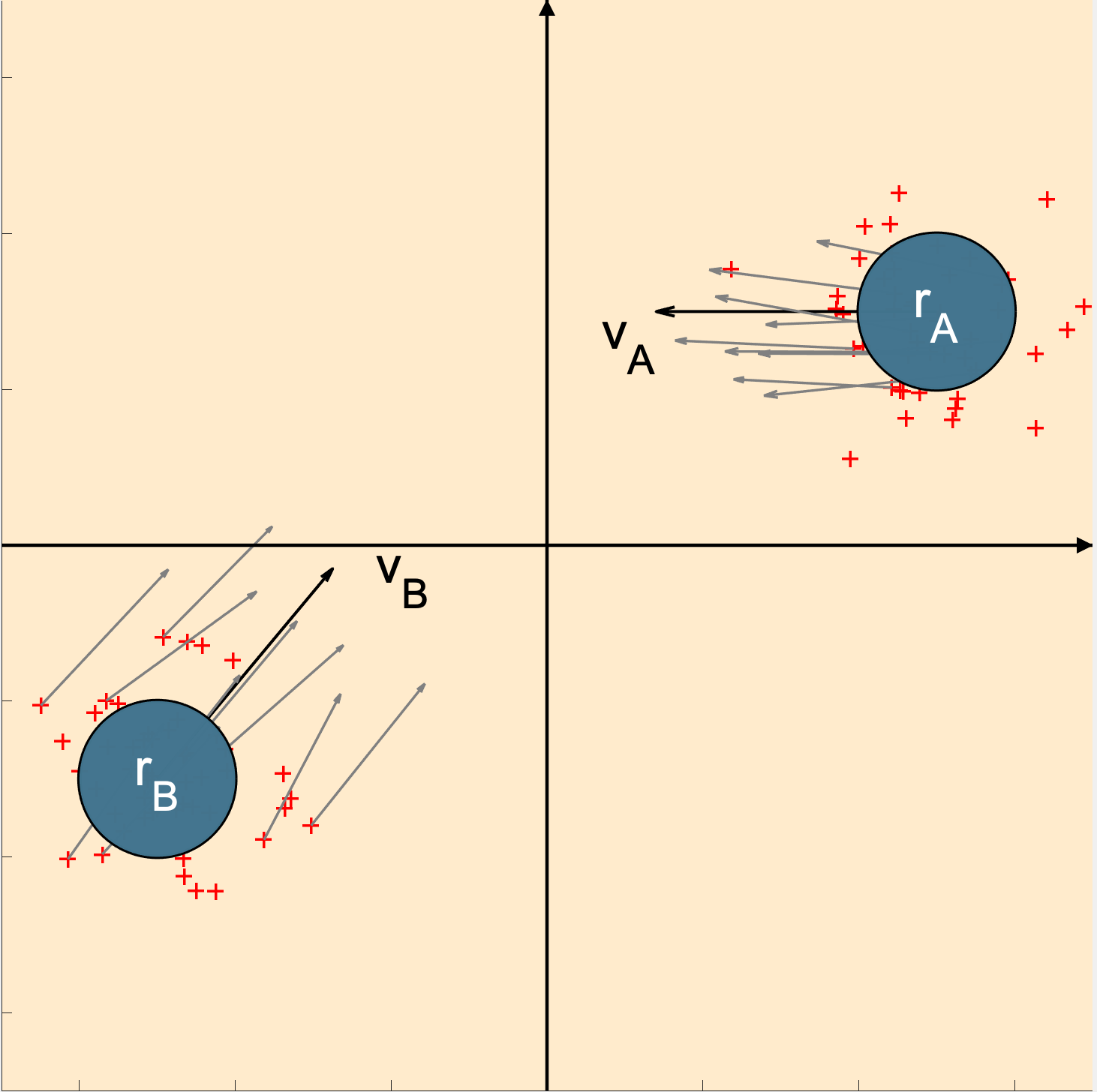
(a) Two-robot scenario

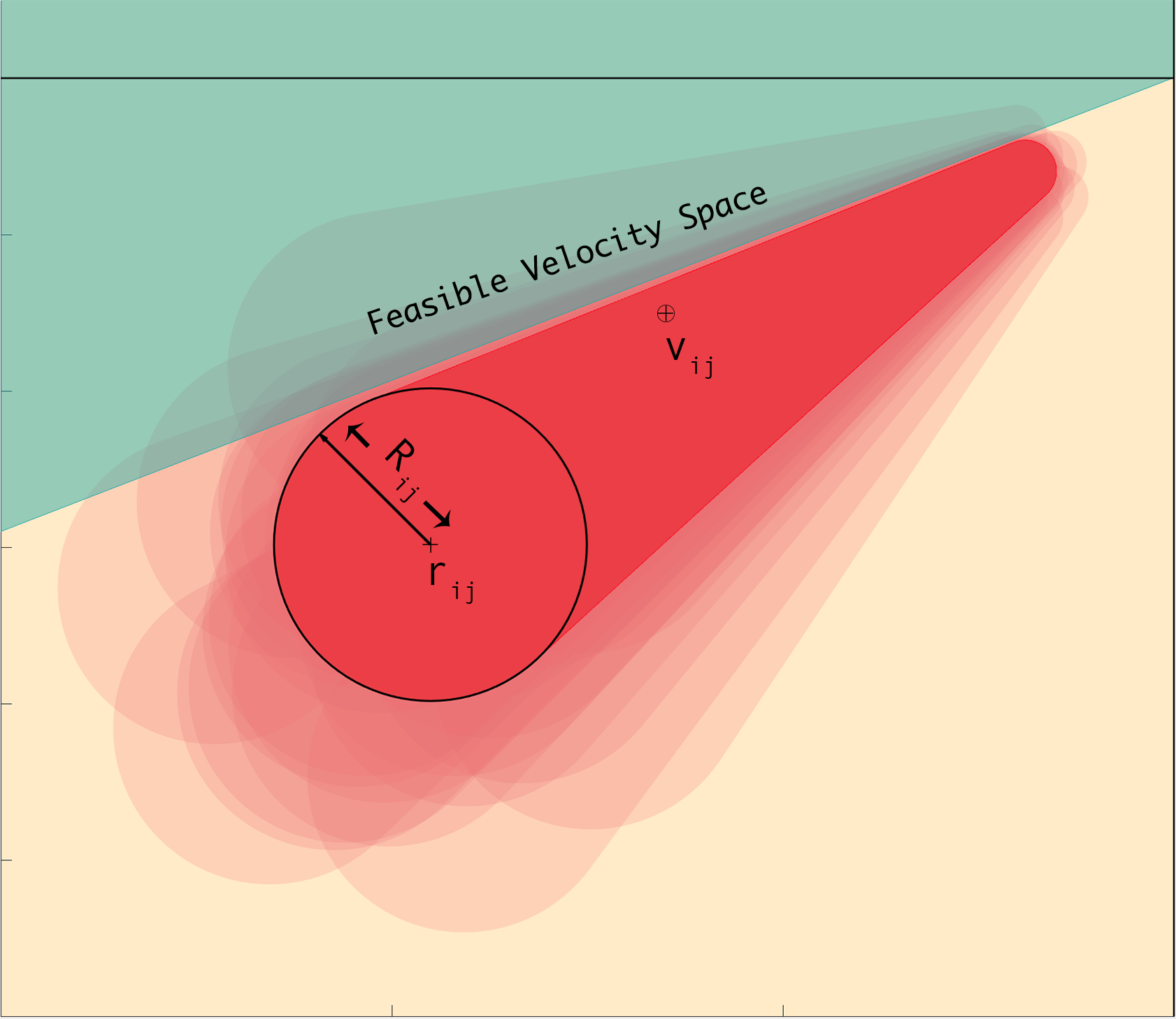
(b) Deterministic ORCA

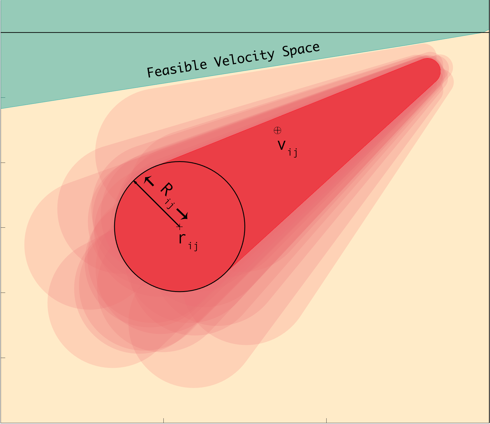
(c) Chance Constrained ORCA

Figure 2: Deterministic and Probabilistic collision avoidance between two agents. (a) Two circular agents with mean positions $r_{i}$ and $r_{j}$ and their respective mean velocities $v_{i}$ and $v_{j}$ (indicated by the black arrow) are shown. The red ‘+’ markers indicate position samples from the position’s uncertainty distribution, and the grey arrows indicate velocity samples from the velocity’s uncertainty distribution. (b) The darker red cone represents the Velocity Obstacle (VO) constructed using the mean position and velocity, while the lighter or translucent red cones represent the VOs constructed from the position and velocity samples from the uncertainty distribution. The green region is the feasible region for the relative velocity computed using ORCA. As can be seen, the green regions overlap with parts of VOs constructed using the position and velocity samples, which can lead to collisions. (c) Feasible relative velocity set computed using the chance constraint ORCA method avoids a major portion of the VO samples.

In this section, we describe our MPC optimization problem and summarize our Gaussian and non-Gaussian chance constraint formulations for collision avoidance. Fig. 2 highlights a 2D scenario for collision avoidance between two agents with state uncertainty. The figure shows a distribution of Velocity Obstacle (VO) cones constructed for the given position and velocity distribution. We observe that the collision-free relative velocity set computed using deterministic ORCA overlaps with a portion of this VO distribution. Hence, a velocity chosen from this set can result in a collision. In contrast, our formulation based on chance constraints results in a feasible relative velocity set that has a higher probability of being collision-free.

IV-A MPC Optimization Setup

We use a receding horizon planner to generate the collision-free trajectories for each quadrotor agent. The underlying optimization framework is common to both our Gaussian and non-Gaussian SwarmCCO formulations. Our Gaussian and non-Gaussian methods differ in the formulation for collision avoidance chance constraints, i.e. the constraint $\text{P}\left({\color[rgb]{0,0,0}{\mathbf{m}^{T}{\mathbf{v}^{orca}_{i}-b\leq 0}}}\right)\leq\delta$ in the optimization is formulated differently (IV-C). Each pair of agents has a constraint $\text{P}\left({\color[rgb]{0,0,0}{\mathbf{m}^{T}{\mathbf{v}^{orca}_{i}-b\leq 0}}}\right)\leq\delta$. That is, if an agent has 5 neighbors, there would be 5 chance constraints in Eqn. (11). The variables $\mathbf{m}$ and $b$ for each constraint would depend on the relative positions and velocities between that pair of agents. For clarity, we have considers a single neighbor case in this section. Each quadrotor agent computes the collision avoidance constraints at each time step and plans a trajectory for the next $N$ time steps. The trajectory is re-planned continuously to account for the changes in the environment.

In our optimization formulation (given below), “$N$” represents the prediction horizon. The weight matrices, Q and R, prioritize between trajectory tracking error and the control input, respectively. $\mathbf{x}_{k}$ represents the state of the agent at time step k, and the matrix A and B are the system matrices for the linearized quadrotor model. Velocity and acceleration are constrained to maximum values, $v_{max}$ and $a_{max}$, respectively, and are realized using box constraints.

$$\underset{}{\text{minimize}}\quad \sum_{t=0}^{N}\left(\mathbf{x}_{ref,t}-\mathbf{x}_{t}\right)Q\left(\mathbf{x}_{ref,t}-\mathbf{x}_{t}\right)+\mathbf{u}_{t}R\mathbf{u}_{t}$$ (11)

subject to $$\mathbf{x}_{0}=\mathbf{x}_{t},$$

$$\mathbf{x}_{k+1}=A\mathbf{x}_{k}+B\mathbf{u}_{k},$$

$$||\mathbf{v}_{k}||\leq v_{max},\ ||\mathbf{a}_{k}||\leq a_{max}$$

$$\text{P}\left({\color[rgb]{0,0,0}{\mathbf{m}^{T}{\mathbf{v}^{orca}_{i}-b\geq 0}}}\right)\geq\delta,$$

$$\forall k=0,1,...,N-1.$$

Our MPC-based algorithm plans in terms of acceleration and yaw rate, which constitute the control input (Section III-D). The constraint $\text{P}\left({\color[rgb]{0,0,0}{\mathbf{m}^{T}{\mathbf{v}^{orca}_{i}-b\leq 0}}}\right)\leq\delta$ represents the chance constraints defined on ORCA, i.e. the constraint is said to be satisfied if, given the uncertainty in state, the probability that the ORCA constraint is satisfied is greater than $\delta$. The output of the MPC is the control input vector for the quadrotor.

IV-B Collision Avoidance Velocity

The VO is constructed using the relative position ($\mathbf{r}_{i}-\mathbf{r}_{j}$) and velocity ($\mathbf{v}_{A}-\mathbf{v}_{B}$) of the agents. From Fig. 2(b), we notice that the ORCA plane passes through the origin. Thus, the parameter $\color[rgb]{0,0,0}{b}$ in the constraint (4) is zero in this case. The feasible velocity set for agent A is constructed by translating this plane by the agent’s mean velocity plus $0.5$ times (as in [6]) the change in relative velocity proposed by ORCA. Due to this translation, $b$ can be non-zero, and we use a mean value for $\color[rgb]{0,0,0}{b}$ instead of a distribution to apply the formulation below.

IV-C Chance Constraint Formulation

Since the position and velocity data of the agent and its neighbors are non-Gaussian random variables, the collision avoidance constraints must consider the uncertainty in the agent’s state estimations for safety. As mentioned in Section III-A, we do not make any assumption on the nature of the uncertainty distribution. However, we model uncertainty using two different methods. Our first method approximates the noise distribution as a Gaussian distribution, which works well for certain sensors. In comparison, our second method is more general and works with non-Gaussian uncertainty by fitting a Gaussian Mixture Model to the uncertainty distribution.
Method I: Gaussian Distribution
In this method, we approximate the position and velocity uncertainties using a multivariate Gaussian distribution. For an agent $i$, its position and velocity variables are approximated as $\mathbf{r}_{i}\sim N(\boldsymbol{\mu}_{i,r},{\Sigma_{i,r}})$, and $\mathbf{v}_{i}\sim N(\boldsymbol{\mu}_{i,v},{\Sigma_{i,v}}).$ The deterministic ORCA constraint between two agents $\color[rgb]{0,0,0}{i}$ and $\color[rgb]{0,0,0}{j}$ is given by the following plane (linear) equation:

$$f^{ORCA_{j}^{i}}(.)={\color[rgb]{0,0,0}{\mathbf{m}^{T}\mathbf{v}^{orca}_{i}-b}}.$$ (12)

Here, the parameters $\color[rgb]{0,0,0}{\mathbf{m}}$ and $\color[rgb]{0,0,0}{b}$ are functions of the agent’s trajectory. In a stochastic setting, the parameters $\color[rgb]{0,0,0}{\mathbf{m}}$ and $\color[rgb]{0,0,0}{b}$ are random variables due to their dependence on the agent’s position and velocity. Though the uncertainty in position and velocity are assumed to be Gaussian for this case, this need not translate to a Gaussian distribution for $\color[rgb]{0,0,0}{\mathbf{m}}$. However, we approximate $\color[rgb]{0,0,0}{\mathbf{m}}$’s distribution as Gaussian for the application of our algorithm, with expectation and covariance represented by $\color[rgb]{0,0,0}{\boldsymbol{\mu}_{\mathbf{m}}}$ and $\color[rgb]{0,0,0}{\Sigma_{\mathbf{m}}}$, respectively. Eqn. (13) highlights the chance constraint, representing the probability that the ORCA constraint (12) is satisfied, given the uncertainties in the position and velocity data. This probability is set to be above a predefined confidence level ($\delta$).

$$\begin{split}P({\color[rgb]{0,0,0}{\mathbf{m}^{T}\mathbf{v}^{orca}_{i}-b\geq 0}})\geq\delta,\ \ {\color[rgb]{0,0,0}{\mathbf{m}\sim N(\boldsymbol{\mu}_{\mathbf{m}},\Sigma_{\mathbf{m}}).}}\end{split}$$ (13)

From [32], we know that if $\mathbf{a}$ follows a Gaussian distribution, the chance constraint can be transformed into a deterministic second-order cone constraint. This is summarized in Lemma IV.1.

Lemma IV.1.

For a multivariate random variable $\color[rgb]{0,0,0}{\mathbf{m}\sim N(\boldsymbol{\mu}_{\mathbf{m}},\Sigma_{\mathbf{m}})}$, the chance constraint $\color[rgb]{0,0,0}{P(\mathbf{m}^{T}\mathbf{x_{t}}\leq b)>\delta}$ can be reformulated as a deterministic constraint on the mean and covariance.

$$\color[rgb]{0,0,0}{P(\mathbf{m}^{T}\mathbf{x}_{t}\leq b)>\delta\iff b-\boldsymbol{\mu}_{\mathbf{m}}^{T}\mathbf{x}_{t}\geq\textnormal{erf}^{-1}(\delta)\left\|{{\Sigma}_{\mathbf{m}}^{\frac{1}{2}}\mathbf{x}_{t}}\right\|_{2}},$$ (14)

where erf(x) is the standard error function given by, $\textnormal{erf}(x)=\frac{1}{2\pi}\int_{0}^{x}e^{-\tau^{2}/2}d\tau.$

Here, $\delta$ is the confidence level associated with satisfying the constraint $\color[rgb]{0,0,0}{\mathbf{m}^{T}\mathbf{x_{t}}\leq b}$. Since our collision avoidance constraints are linear, each chance constraint can be reformulated to a second order cone constraint, as shown in Lemma IV.1. Hence, each collision avoidance chance constraint can be written as

$${\color[rgb]{0,0,0}{P(\mathbf{m}^{T}\mathbf{v}_{i}^{orca}-b\geq 0)\geq\delta}}\iff\\ {\color[rgb]{0,0,0}{\boldsymbol{\mu}_{\mathbf{m}}^{T}\mathbf{v}_{i}^{orca}-b+\textnormal{erf}^{-1}(\delta)\left\|{{\Sigma}_{\mathbf{m}}^{\frac{1}{2}}\mathbf{v}_{i}^{orca}}\right\|_{2}\leq 0.}}$$ (15)

Method II: Gaussian Mixture Model (GMM)
To handle non-Gaussian uncertainty distributions, we present an extension of the Gaussian formulation (Method I). In this case, the probability distribution for the position and velocity is assumed to be non-parametric and non-Gaussian, i.e. the probability distribution is not known. We assume that we have access to ${\color[rgb]{0,0,0}s}$ samples of these states that could come from a black-box simulator or a particle filter. Using ${\color[rgb]{0,0,0}s}$ samples, a distribution for the parameter $\color[rgb]{0,0,0}{\mathbf{m}}$ is constructed. In our implementation, we use a value of ${\color[rgb]{0,0,0}s}=40$ samples.

A GMM model of ${\color[rgb]{0,0,0}n}$ Gaussian components is fit to the probability distribution of parameter $\color[rgb]{0,0,0}{\mathbf{m}}$ in Eqn. 12 using Expectation-Maximization (EM). Each collision avoidance constraint is split into ${\color[rgb]{0,0,0}n}$ second-order constraints, each corresponding to a single Gaussian component. Furthermore, an additional constraint is used that relates the $\mathbf{n}$ second-order constraints to GMM probability distribution. From [33], we know that if $\color[rgb]{0,0,0}{\mathbf{m}}$ follows a GMM distribution, the chance constraint can be transformed into a set of deterministic constraints. This is summarized in Lemma IV.2.

Lemma IV.2.

For a non-Gaussian random variable $\color[rgb]{0,0,0}{\mathbf{m}}$ and a linear equation $f(\mathbf{x_{t}})=\color[rgb]{0,0,0}{\mathbf{m}^{T}\mathbf{x_{t}}\leq b}$, the chance constraint $P({\color[rgb]{0,0,0}{\mathbf{m}^{T}\mathbf{x_{t}}\leq b}})>\delta$ can be reformulated as a set of deterministic constraints on the mean and co-variance. Let the distribution of $\color[rgb]{0,0,0}{\mathbf{m}}$ be approximated by $\mathbf{n}$ Gaussian components. The probability that $f(\mathbf{x_{t}})$ is satisfied while $\color[rgb]{0,0,0}{\mathbf{m}}$’s distribution is given by the $n^{th}$ Gaussian component of the GMM is given by

$${\color[rgb]{0,0,0}{P_{i}=\textnormal{erf}\bigg{(}\frac{b-\boldsymbol{\mu}_{\mathbf{m}}^{T}\mathbf{x}_{t}}{\sqrt{\mathbf{x_{t}}^{T}\Sigma_{\mathbf{m}}\mathbf{x_{t}}}}\bigg{)}.}}$$ (16)

Then, the probability that $f(\mathbf{x_{t}})$ is satisfied for GMM distribution of $\color[rgb]{0,0,0}{\mathbf{m}}$ is given by

$$P_{GMM}=\sum_{i=1}^{n}{\color[rgb]{0,0,0}\alpha_{i}P_{i}}.$$ (17)

Here, ${\color[rgb]{0,0,0}\alpha_{i}}$s are the mixing coefficients for the GMM, satisfying $\sum_{i=1}^{n}{\color[rgb]{0,0,0}\alpha_{i}}=1$.

Let us assume that the probability of satisfying $\color[rgb]{0,0,0}{\mathbf{m}^{T}\mathbf{v}_{i}^{orca}-b\geq 0,}$ while considering only the $n^{th}$ Gaussian component, is given by $\eta_{i}$. We can reformulate the constraint using Lemma IV.2, which is given by Eqn. 18.

The probability of satisfying the linear constraint considering the GMM distribution for $\color[rgb]{0,0,0}{\mathbf{m}}$ is computed by mixing the individual component probabilities using the mixing coefficients ($\alpha_{i}$). A probability $\delta$ is chosen as the required confidence level. Eqn. (19) represents the chance constraint that the probability of satisfying Eqn. (12) is greater than $\delta$. The chance constraint can be reformulated as:

(18)

$$\leavevmode\resizebox{108.405pt}{}{$\sum_{i=1}^{n}{\color[rgb]{0,0,0}{\alpha_{i}\eta_{i}>\delta}}$}.$$ (19)

In Eqn. 19 the values for the mixing coefficient and confidence are known prior to the optimization. We notice that for a given set of mixing coefficients ($\alpha_{i}$s) and confidence ($\delta$), multiple sets of values for $\eta_{i}$’s can satisfy Eqn. 19. The value of $\eta_{i}$ in turn affects the feasible velocity set. Hence, we plan for $\eta_{i}$’s in addition to the control input in problem (Equation 11). When GMM has 3 components, i.e. ${n}=3$, we have three additional variables given by $\eta_{1},\eta_{2},\eta_{3}$ in the optimization problem. Now the optimization problem (Equation 11) simultaneously computes values for acceleration, $\dot{\psi}$ and $\eta_{i}$, such that the collision avoidance chance constraints (Eqn. 19) are satisfied.

The computed control input from the optimization problem (11) is transformed into an inner-loop control input for the quadrotor using an inverse map, similar to [15].

V Results

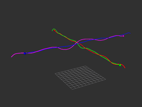
(a) DCAD(Deterministic)

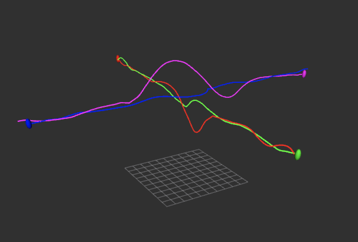
(b) Gaussian Noise Approximation

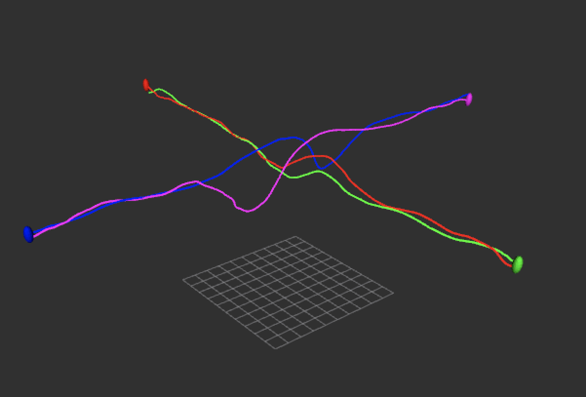
(c) Non-Gaussian Noise Approximation

Figure 3: The figure illustrates a scenario with 4 agents exchanging positions with their diagonally opposite agents. The collision avoidance is performed based on deterministic DCAD and Gaussian and non-Gaussian SwarmCCO. DCAD results in more collisions because uncertainty is not explicitly considered. We observe that some agents travel a longer path when using the Gaussian formulation than when using the non-Gaussian formulation (Section V-D1).

In this section, we describe the implementation of our algorithm and our simulation setup. Further, we summarize our evaluations and highlight the benefits of our approach.

V-A Experimental Setup

Our method is implemented on an Inter Xeon w-2123 3.6 GHz with 32 GB RAM and a GeForce GTX 1080 GPU. Our simulations are built using the PX4 Software In The Loop (SITL) framework, ROS Kinetic, and Gazebo 7.14.0. We solve the MPC optimization using the IPOPT Library with a planning horizon of $N=8$ steps and a time step of $\delta$t = $100$ms. We consider a non-Gaussian distribution for the position and velocity data, from which the input sensor readings for both the Gaussian and non-Gaussian SwarmCCO methods are generated. Gazebo state information represents the ground truth position and velocity data, while we add non-zero mean, non-Gaussian noise to simulate state uncertainties. The added noise is generated through a GMM model of 3 Gaussian components. We use two different GMM to simulate noise for position readings: $GMM_{1}:\mu_{GMM1}=[0.15,0.08,-0.05]$, $\Sigma_{GMM1}=diag([0.06,0.7,0.3])$, and $GMM_{2}:\mu_{GMM2}=[0.2,0.0,-0.2]$, $\Sigma_{GMM2}=diag([1.0,0.3,1.0])$. The velocity readings are simulated using a noise distribution that has half the mean and covariance values of $\Sigma_{GMM1}$ and $\Sigma_{GMM2}$. Further, for our evaluation we consider two confidence levels given by $\delta_{1}=0.75$ and $\delta_{2}=0.90$. The RVO-3D library is utilized to compute the ORCA collision avoidance constraints. We consider a sensing region of 8m for the ORCA plane computation. The agent’s physical radius is assumed to be $0.25m$ while the agent’s radius for the ORCA computation is set as $0.5m$. In our evaluations, two agents are considered to be in collision if their positions are less than $0.5m$ apart. Further, we show results for the non-Gaussian method with 2 components ($n=2$) GMM and 3 components ($n=3$) GMM.

V-B Generated Trajectories

We evaluate our method in simulation with four quadrotors exchanging positions with the antipodal agents (circular scenario). Fig. 3 shows the resulting trajectories for this scenario using deterministic DCAD [15] and Gaussian and non-Gaussian SwarmCCO. We observe that in deterministic DCAD, the agents do not handle noise and hence they trajectories often result in collisions. In Fig. 3 the DCAD trajectories are such that the agent graze past each other. In contrast, the trajectories generated by SwarmCCO methods are safer.

V-C Collision Avoidance

Table II: Number of episodes in which one or more quadrotor collided when the agents out of a total of 100 episodes. The DCAD algorithm is deterministic and does not consider the uncertainty in state. We observe that our Gaussian and non-Gaussian formulations provide improved safety.

Noise	Confidence Level	Method	Number of collisions
			No of Agents
			2	4	6	8	10
$\Sigma_{1}$	$\delta=0.75$	DCAD (deterministic)	27	25	35	40	44
		Gaussian SwarmCCO	0	4	4	7	15
		Non-Gaussian SwarmCCO (n=2)	0	2	5	4	12
		Non-Gaussian SwarmCCO (n=3)	0	0	2	5	13
	$\delta=0.90$	DCAD (deterministic)	27	25	35	40	44
		Gaussian SwarmCCO	0	3	2	7	13
		Non-Gaussian SwarmCCO (n=2)	0	1	3	4	12
		Non-Gaussian SwarmCCO (n=3)	0	0	1	2	10
$\Sigma_{2}$	$\delta=0.75$	DCAD (deterministic)	56	26	32	51	58
		Gaussian SwarmCCO	0	2	3	11	18
		Non-Gaussian SwarmCCO (n=2)	0	1	3	5	9
		Non-Gaussian SwarmCCO (n=3)	0	0	0	3	10
	$\delta=0.90$	DCAD (deterministic)	56	26	32	51	58
		Gaussian SwarmCCO	0	2	1	4	6
		Non-Gaussian SwarmCCO (n=2)	0	0	1	3	4
		Non-Gaussian SwarmCCO (n=3)	0	0	0	2	4

We evaluate our method in a circular scenario. Table II summarizes the number of trials with observed collisions out of a total of 100 trials. We observe that the performance of the deterministic method degrades (in terms of number of collisions) with added noise. In contrast, we observe good performance with both the Gaussian and non-Gaussian SwarmCCO. As expected, the number of collisions reduces with an increase in confidence level ($\delta$).

V-D Gaussian vs. Non-Gaussian:

In this subsection we compare the performance of our Gaussian and non-Gaussian formulations for SwarmCCO. We consider the circular scenario where the agents move to their antipodal positions.

V-D1 Path Length

Table III: Average path length traveled by the agent while exchanging positions with the antipodal agents. The reference, straight line path to the goal is $40$m long. The Gaussian method is relatively conservative, resulting in longer path lengths on average compared to the non-Gaussian method. We observe this performance in scenarios with 8 and 10 agents.

Noise	Confidence Level	Method	Path Length
			No of Agents
			2	4	6	8	10
$\Sigma_{1}$	$\delta=0.75$	Gaussian	41.12	42.75	44.04	44.88	47.92
		Non-Gaussian (n=2)	41.06	41.95	43.03	44.39	46.66
		Non-Gaussian (n=3)	41.06	42.09	43.12	44.59	46.52
	$\delta=0.90$	Gaussian	41.10	43.14	45.05	46.64	48.87
		Non-Gaussian (n=2)	41.07	42.03	43.31	44.42	46.53
		Non-Gaussian (n=3)	41.06	42.12	43.35	44.57	46.62
$\Sigma_{2}$	$\delta=0.75$	Gaussian	41.21	43.06	44.51	46.38	49.61
		Non-Gaussian (n=2)	41.21	42.67	44.09	45.80	47.87
		Non-Gaussian (n=3)	41.22	42.47	44.14	45.93	48.15
	$\delta=0.90$	Gaussian	41.23	43.69	45.37	47.90	50.41
		Non-Gaussian (n=2)	41.21	42.47	44.13	45.68	48.09
		Non-Gaussian (n=3)	41.23	42.70	44.62	46.13	48.25

Table IV: Mean time required by the agents to reach the goal. The mean time required is approximately the same for all the methods due to the trajectory tracking MPC uses in our formulation.

Method	$\Sigma_{1}$								$\Sigma_{2}$
	$\delta=0.75$				$\delta=0.90$				$\delta=0.75$				$\delta=0.90$
	2	4	6	8	2	4	6	8	2	4	6	8	2	4	6	8
Gaussian	31.41	31.41	31.41	31.42	31.41	31.42	31.41	31.41	31.41	31.41	31.42	31.43	31.41	31.41	31.41	31.42
Non-Gaussian (n=2)	31.41	31.41	31.41	31.42	31.41	31.42	31.41	31.41	31.41	31.41	31.42	31.41	31.41	31.41	31.41	31.41
Non-Gaussian (n=3)	31.41	31.41	31.41	31.42	31.41	31.42	31.41	31.41	31.41	31.41	31.42	31.41	31.41	31.41	31.41	31.42

For each agent, the reference path to its goal is a straight-line path of 40m length directed to the diametrically opposite position. In Table III, we tabulate the mean path length for the agents as they reach their goal while avoiding collisions. To compute this mean, we utilize only the trials that were collision-free. The mean is computed over 100 trials. We observe that the Gaussian method is (relatively) more conservative than the non-Gaussian method resulting in a longer path length for most scenarios.

V-D2 Time to Goal

We observe that on average, the agents in all the methods reach their goal in the same time, this can be observed from Table IV. This is due to the trajectory tracking MPC used by the agents, which modifies the agent velocity such that the agents reach their goal in approximately the same time duration ($\sim 30s$).

V-D3 Inter-agent Distance

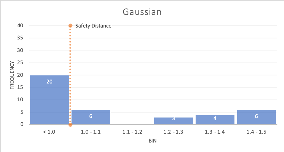
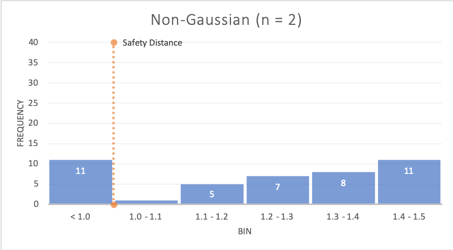
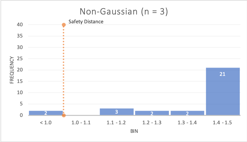
(a) Scenario with four agents.

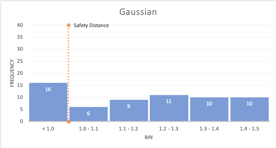
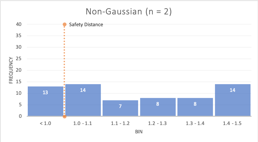
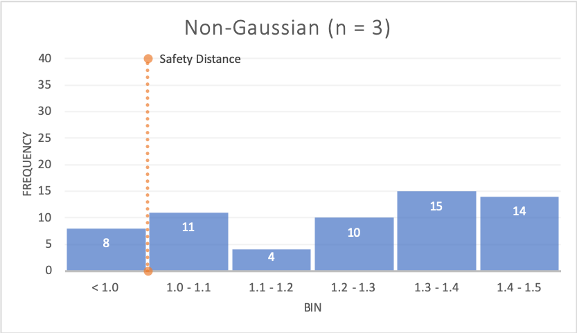
(b) Scenario with six agents.

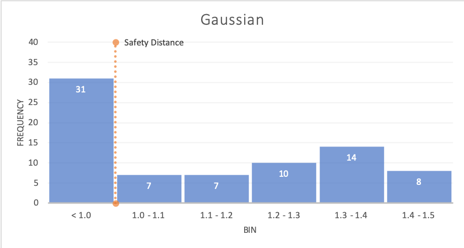
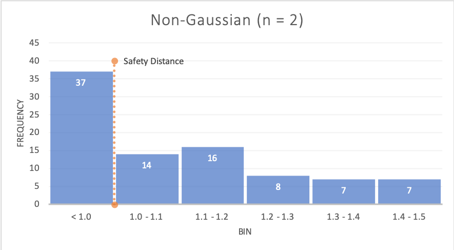
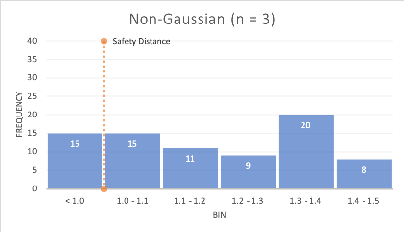
(c) Scenario with eight agents.

Figure 4: Histogram of least inter-agent distance in the circular scenario with 4, 6 and 8 agents. The agents have a radius of $0.25m$, and the ORCA planes are constructed with an augmented agent radius of $0.5m$. Hence, an inter-agent distance of less than $1m$ is a collision according to the ORCA constraint, though the agents do not actually collide. The histogram is constructed over 100 trials, and the trials with least inter-agent distance greater than $1.5m$ are not included in the histogram. The safe inter-agent distance of $1m$ is denoted by the dotted orange line. We observe that the non-Gaussian method results in fewer trials with least inter-agent distance below $1m$, especially for the non-Gaussian formulation with 3 components.

In the ORCA computation, the agent radius is augmented to be $0.5m$ in contrast to the original agent radius of $0.25m$ to provide a safe distance around the agent. Thus, the safe inter-agent distance is $1m$. We compare the Gaussian and non-Gaussian formulations for the number of trials in which the safety threshold distance was compromised (out of 100 trials). We observe that the non-Gaussian method performs better in this case, and the results are illustrated through a histogram in Fig. 4. We observe that with an increase in the number of agents in the environment, the inter-agent distance dips below $1m$ in multiple trials, but the non-Gaussian method with 3 Gaussian components performs better resulting in lower number of such trials.

V-E Scalability

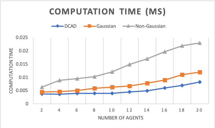
Figure 5: Control input computation time (ms) for one agent in the presence of 2 to 20 neighboring agents.

Figure 5 illustrates the computation time (in milliseconds) of our algorithm for one agent with $1$ to $20$ neighbouring agents in the environment. From our previous work [15], and from our experiments we observe that considering the closest 10 obstacles provides good performance in most cases. We observe that, on average, our Gaussian method requires $\sim 5ms$ to compute a collision avoiding input, while our non-Gaussian method requires $\sim 7ms$ in the presence of $4$ neighbors.

V-F Comparision with Bounding Volume Expansion

In Table V, we compare the non-Gaussian formulation with a conservative method based on bounding volume expansion (DCAD [15]). We observed the bounding volume formulation returned infeasible frequently owing to its conservative approximation. This was observed for the $8$ and $10$ agent cases. A 100 trial runs in the circular scenario was used to tabulate this result. Thus, a conservative method may not be practical in all scenarios.

Method	Path Length					No. of trials with collision
	2	4	6	8	10	2	4	6	8	10
DCAD with Kalman filter	41.39	45.47	61.83	-	-	0	0	4	-	-
non-Gaussian SwarmCCO (n=2)	41.24	45.34	47.29	51.30	57.90	0	0	0	6	11

Table V: Comparison of average path length and collision prbability between DCAD (kalman filter) and non-Gaussian SwarmCCO

VI Conclusion, Limitation, and Future Work

In this paper, we presented a probabilistic method for decentralized collision avoidance among quadrotors in a swarm. Our method uses a flatness-based linear MPC to handle quadrotor dynamics and accounts for the state uncertainties using a chance constraint formulation. We presented two approaches to model the chance constraints; the first assumes a Gaussian distribution for the state, while the second approach is more general and can handle non-Gaussian noise using a GMM. Both the Gaussian and non-Gaussian methods result in fewer collisions as compared to the deterministic algorithms, but the Gaussian method was found to be more conservative, leading to longer path lengths for the agents. Further, we observed that the non-Gaussian method with 3 Gaussian components demonstrates better performance in terms of satisfying the ORCA constraints, resulting in fewer trials with an inter-agent safety distance lower than $1m$ compared to the Gaussian formulation. On average, our Gaussian method required $\sim 5ms$ to compute a collision avoiding input, while our non-Gaussian method requires $\sim 9ms$ in scenarios with $4$ agents.

Our method has a few limitations. We estimate the distribution of $\mathbf{m}$ using position and velocity samples from a black-box simulator, hence the distribution may not be accurate. The non-Gaussian method is computationally expensive, which affects the rapid re-planning of trajectories. In addition, we do not consider the ego-motion noise, i.e. the noise in implementing the control input. Moreover, our optimization’s cost function uses mean values and does not consider the uncertainties in the state.

As a part of our future work, we plan to work on faster methods to evaluate the chance constraint for the non-Gaussian, non-parametric case. Additionally, we plan to evaluate our algorithm on physical quadrotors.

References

- [1] F. Augugliaro, A. P. Schoellig, and R. D’Andrea, “Generation of collision-free trajectories for a quadrocopter fleet: A sequential convex programming approach,” in 2012 IEEE/RSJ international conference on Intelligent Robots and Systems. IEEE, 2012, pp. 1917–1922.
- [2] A. Kushleyev, D. Mellinger, C. Powers, and V. Kumar, “Towards a swarm of agile micro quadrotors,” Autonomous Robots, vol. 35, no. 4, pp. 287–300, 2013.
- [3] J. A. Preiss, W. Hönig, N. Ayanian, and G. S. Sukhatme, “Downwash-aware trajectory planning for large quadrotor teams,” in 2017 IEEE/RSJ International Conference on Intelligent Robots and Systems (IROS). IEEE, 2017, pp. 250–257.
- [4] P. Fiorini and Z. Shiller, “Motion planning in dynamic environments using velocity obstacles,” The International Journal of Robotics Research, vol. 17, no. 7, pp. 760–772, 1998.
- [5] J. Van den Berg, M. Lin, and D. Manocha, “Reciprocal velocity obstacles for real-time multi-agent navigation,” in 2008 IEEE International Conference on Robotics and Automation. IEEE, 2008, pp. 1928–1935.
- [6] J. Van Den Berg, S. J. Guy, M. Lin, and D. Manocha, “Reciprocal n-body collision avoidance,” in Robotics research. Springer, 2011, pp. 3–19.
- [7] D. Morgan, S.-J. Chung, and F. Y. Hadaegh, “Decentralized model predictive control of swarms of spacecraft using sequential convex programming,” Advances in the Astronautical Sciences, no. 148, pp. 1–20, 2013.
- [8] D. Zhou, Z. Wang, S. Bandyopadhyay, and M. Schwager, “Fast, on-line collision avoidance for dynamic vehicles using buffered voronoi cells,” IEEE Robotics and Automation Letters, vol. 2, no. 2, pp. 1047–1054, April 2017.
- [9] K. Khoshelham and S. O. Elberink, “Accuracy and resolution of kinect depth data for indoor mapping applications,” Sensors, vol. 12, no. 2, pp. 1437–1454, 2012.
- [10] J. S. Park and D. Manocha, “Efficient probabilistic collision detection for non-gaussian noise distributions,” IEEE Robotics and Automation Letters, 2020.
- [11] J. Snape, J. Van Den Berg, S. J. Guy, and D. Manocha, “The hybrid reciprocal velocity obstacle,” IEEE Transactions on Robotics, vol. 27, no. 4, pp. 696–706, 2011.
- [12] M. Kamel, J. Alonso-Mora, R. Siegwart, and J. Nieto, “Robust collision avoidance for multiple micro aerial vehicles using nonlinear model predictive control,” in 2017 IEEE/RSJ International Conference on Intelligent Robots and Systems (IROS). IEEE, 2017, pp. 236–243.
- [13] H. Zhu and J. Alonso-Mora, “Chance-constrained collision avoidance for mavs in dynamic environments,” IEEE Robotics and Automation Letters, vol. 4, no. 2, pp. 776–783, 2019.
- [14] B. Gopalakrishnan, A. K. Singh, M. Kaushik, K. M. Krishna, and D. Manocha, “Prvo: Probabilistic reciprocal velocity obstacle for multi robot navigation under uncertainty,” in 2017 IEEE/RSJ International Conference on Intelligent Robots and Systems (IROS), Sep. 2017, pp. 1089–1096.
- [15] S. H. Arul and D. Manocha, “Dcad: Decentralized collision avoidance with dynamics constraints for agile quadrotor swarms,” IEEE Robotics and Automation Letters, pp. 1–1, 2020.
- [16] J. Van Den Berg, J. Snape, S. J. Guy, and D. Manocha, “Reciprocal collision avoidance with acceleration-velocity obstacles,” in 2011 IEEE International Conference on Robotics and Automation. IEEE, 2011, pp. 3475–3482.
- [17] M. Rufli, J. Alonso-Mora, and R. Siegwart, “Reciprocal collision avoidance with motion continuity constraints,” IEEE Transactions on Robotics, vol. 29, no. 4, pp. 899–912, 2013.
- [18] J. Van Den Berg, D. Wilkie, S. J. Guy, M. Niethammer, and D. Manocha, “Lqg-obstacles: Feedback control with collision avoidance for mobile robots with motion and sensing uncertainty,” in 2012 IEEE International Conference on Robotics and Automation. IEEE, 2012, pp. 346–353.
- [19] D. Bareiss and J. Van den Berg, “Reciprocal collision avoidance for robots with linear dynamics using lqr-obstacles,” in 2013 IEEE International Conference on Robotics and Automation. IEEE, 2013, pp. 3847–3853.
- [20] H. Cheng, Q. Zhu, Z. Liu, T. Xu, and L. Lin, “Decentralized navigation of multiple agents based on orca and model predictive control,” in 2017 IEEE/RSJ International Conference on Intelligent Robots and Systems (IROS). IEEE, 2017, pp. 3446–3451.
- [21] B. Gopalakrishnan, A. K. Singh, M. Kaushik, K. M. Krishna, and D. Manocha, “Chance constraint based multi agent navigation under uncertainty,” in Proceedings of the Advances in Robotics, 2017, pp. 1–6.
- [22] G. Angeris, K. Shah, and M. Schwager, “Fast reciprocal collision avoidance under measurement uncertainty,” 2019.
- [23] H. Zhu and J. Alonso-Mora, “B-uavc: Buffered uncertainty-aware voronoi cells for probabilistic multi-robot collision avoidance,” in 2019 International Symposium on Multi-Robot and Multi-Agent Systems (MRS), Aug 2019, pp. 162–168.
- [24] P. S. N. Jyotish, B. Gopalakrishnan, A. V. S. S. Bhargav Kumar, A. K. Singh, K. M. Krishna, and D. Manocha, “Reactive navigation under non-parametric uncertainty through hilbert space embedding of probabilistic velocity obstacles,” IEEE Robotics and Automation Letters, pp. 1–1, 2020.
- [25] R. B. Rusu, I. Alexandru, B. Gerkey, S. Chitta, M. Beetz, L. E. Kavraki, et al., “Real-time perception-guided motion planning for a personal robot,” in 2009 IEEE/RSJ International Conference on Intelligent Robots and Systems. IEEE, 2009, pp. 4245–4252.
- [26] A. Lee, Y. Duan, S. Patil, J. Schulman, Z. McCarthy, J. van den Berg, K. Goldberg, and P. Abbeel, “Sigma hulls for gaussian belief space planning for imprecise articulated robots amid obstacles,” in Intelligent Robots and Systems (IROS), 2013 IEEE/RSJ International Conference on. IEEE, 2013, pp. 5660–5667.
- [27] N. E. Du Toit and J. W. Burdick, “Probabilistic collision checking with chance constraints,” Robotics, IEEE Transactions on, vol. 27, no. 4, pp. 809–815, 2011.
- [28] C. Park, J. S. Park, and D. Manocha, “Fast and bounded probabilistic collision detection in dynamic environments for high-dof trajectory planning,” arXiv preprint arXiv:1607.04788, proceedings of Workshop on the Algorithmic Foundations of Robotics (WAFR), 2016.
- [29] D. Mellinger and V. Kumar, “Minimum snap trajectory generation and control for quadrotors,” in 2011 IEEE International Conference on Robotics and Automation, 2011, pp. 2520–2525.
- [30] J. Ferrin, R. Leishman, R. Beard, and T. McLain, “Differential flatness based control of a rotorcraft for aggressive maneuvers,” in 2011 IEEE/RSJ International Conference on Intelligent Robots and Systems, 2011, pp. 2688–2693.
- [31] A. Charnes and W. W. Cooper, “Chance-constrained programming,” Management Science, vol. 6, no. 1, pp. 73–79, 1959. [Online]. Available: http://www.jstor.org/stable/2627476
- [32] A. Prékopa, Stochastic programming. Springer Science & Business Media, 2013, vol. 324.
- [33] Z. Hu, W. Sun, and S. Zhu, “Chance constrained programs with mixture distributions,” 2018.