Spot Patterns in the 2-D Schnakenberg Model with Localized Heterogeneities

Abstract

A hybrid asymptotic-numerical theory is developed to analyze the effect of different types of localized heterogeneities on the existence, linear stability, and slow dynamics of localized spot patterns for the two-component Schnakenberg reaction-diffusion model in a 2-D domain. Two distinct types of localized heterogeneities are considered: a strong localized perturbation of a spatially uniform feed rate and the effect of removing a small hole in the domain, through which the chemical species can leak out. Our hybrid theory reveals a wide range of novel phenomena such as, saddle-node bifurcations for quasi-equilibrium spot patterns that otherwise would not occur for a homogeneous medium, a new type of spot solution pinned at the concentration point of the feed rate, spot self-replication behavior leading to the creation of more than two new spots, and the existence of a creation-annihilation attractor with at most three spots. Depending on the type of localized heterogeneity introduced, localized spots are either repelled or attracted towards the localized defect on asymptotically long time scales. Results for slow spot dynamics and detailed predictions of various instabilities of quasi-equilibrium spot patterns, all based on our hybrid asymptotic-numerical theory, are illustrated and confirmed through extensive full PDE numerical simulations.

keywords — Pattern formation, reaction-diffusion systems, spots, localized heterogeneites, pinning.

1 Introduction

Localized spot patterns, in which a solution component becomes spatially localized near certain time-varying discrete points within a bounded multi-dimensional domain, is a well-known “far-from-equilibrium” spatial pattern that occurs for certain two-component reaction-diffusion (RD) systems in the singular limit of a large diffusivity ratio. This class of localized pattern is observed in many chemical and biological systems, such as the chlorine-dioxide-malonic acid reaction [9], the ferrocyanide-iodate-sulphite reaction [25, 26], and the initiation of plant root hair cells mediated by the plant hormone auxin [2], among others (see [36] and [14] for surveys). In a spatially homogeneous 2-D medium, and for various specific RD systems, the slow dynamical behavior of quasi-equilibrium spot patterns, together with their various types of bifurcations that trigger a range of different instabilities of the pattern such as spot-annihilation, spot-replication, and temporal oscillations of the spot amplitude, have been well-studied [7, 17, 31, 32, 33, 40, 41, 42, 47]. The primary focus of this article is to investigate, for one prototypical RD system, how certain spatial heterogeneities in the model affect the dynamics and instabilities of quasi-equilibrium spot patterns, and lead to new dynamical phenomena that would otherwise not occur in a medium free of defects. For tractability of our analysis, and as we describe below, we will focus only on certain types of spatially localized heterogeneities.

There is a growing literature, primarily in a 1-D setting, of analyzing the effect of a spatial heterogeneity in either the diffusivity or reaction kinetics on pattern-formation behavior for two-component RD systems with regards to both small amplitude patterns (see [29], [30], [23] and the references therein) and for localized far-from-equilibrium spike-type patterns (cf. [2], [3], [4], [5], [10], [18], [19], [20], [21], [33], [39], [43], [44], [45]). In particular, the analysis in [21] and [43] has revealed that a precursor gradient in the reaction kinetics can lead to the existence of stable asymmetric spike patterns for the Gierer-Meinhardt (GM) model, which would otherwise not occur in a homogeneous medium. A precursor field for the GM model can also lead to stable steady-states consisting of spike clusters near critical points of the precursor. In [22] it was shown that a different type of smooth heterogeneity in the 1-D GM model can lead to the formation of a creation-annihilation attractor, which consists of periodically repeating cycles of spike formation, propagation, and annihilation against a domain boundary. In the limit of a large number of spikes that are confined by a spatial heterogeneity, a mean field equation for the spike density was derived in [20] and [18] for the 1-D GM and Schnakenberg models, respectively, and in [19] for 2-D spot clusters for the GM model. For the 1-D Schnakenburg model, the mean field limiting equation in [18] revealed the existence of a creation-annihilation attractor in which spikes undergo self-replication in the interior of the spike cluster, while other spikes are annihilated at the edges of the cluster. For an extended Klausmeir RD model of spatial ecology, coarsening and pinning behavior of 1-D spike patterns with various spatial and temporal heterogeneities were analyzed in [3] and [4]. Spike dynamics and pinning effects for a 1-D RD model where the nonlinearities have small spatial support, as is typical for catalytic reactions, was studied in [10].

For a different class of localized pattern consisting of either a propagating pulse-type or a transition-layer solution, there has been much effort at analyzing the effect of a small step function barrier on pulse propagation properties for the three-component Fitzhugh-Nagumo RD system (cf. [6], [35], [34], [48]) and for two-component bistable RD systems (cf. [11], [27]). For this type of jump-type spatial heterogeneity, the focus has been to analytically determine parameter ranges where a 1-D propagating pulse will either be reflected, transmitted, or pinned by the barrier. In a 2-D setting, [28] provides a numerical study of similar propagation and collision properties for a single localized spot in the presence of a 1-D step-function line barrier.

In contrast to the simpler 1-D case, there are relatively few analytical studies of the effect of spatial heterogeneities for RD systems in higher spatial dimensions. For a generalized Schnakenberg-type RD system modeling the initiation of root hair profusion in plant cells, a spatially inhomogeneous auxin gradient in a 2-D rectangular domain was shown to lead to the alignment of localized spots in the direction of the gradient (cf. [2]). In a 2-D rectangular domain, it was shown in [16] for a generalized Klausmeir RD system, modeling vegetation patterns in semi-arid environments, that an anisotropic diffusivity can stabilize a localized stripe pattern to transverse perturbations. With isotropic diffusion, the homoclinic stripe would be unstable to either breakup into spots or zigzag deformations. Spot-pinning behavior for RD systems on closed manifolds of non-constant curvature, which can be viewed as intrinsic spatial heterogeneities, has been analyzed for the Schnakenberg model in [13]. In [33], which is most closely related to our study, the role of Robin boundary conditions and boundary fluxes on the slow dynamics and instabilities of quasi-equilibrium spot patterns for the Brusselator RD model was analyzed.

The goal of this paper is to analyze the effect of various types of localized heterogeneities for the singularly perturbed Schnakenberg model in a bounded 2-D domain $\Omega$, formulated as

$$v_{t}=\varepsilon^{2}\Delta v-v+uv^{2}\,,\quad\tau u_{t}=D\Delta u+a-\varepsilon^{-2}uv^{2}\,,\quad\mathbf{x}\in\Omega\,;\qquad\partial_{n}v=\partial_{n}u=0\,,\quad\mathbf{x}\in\partial\Omega\,,$$ (1.1)

where $0<\varepsilon\ll 1$, while $D>0$ and $\tau>0$ are ${\mathcal{O}}(1)$ constants. One heterogeneity will be introduced through strong, but local, perturbations in the feed rate $a=a(\mathbf{x})$, which characterizes the amount of material that is introduced from the substrate. Another localized heterogeneity that we will consider is to analyze the effect of perturbing (1.1) by removing a small hole in the domain, which thereby allows leakage of the chemical species out of the domain.

For these types of localized heterogeneities we will extend the hybrid asymptotic-numerical framework of [17] and [33] to analyze the existence, linear stability, and slow dynamics of quasi-equilibrium spot patterns. Depending on the type of localized heterogeneity introduced, spot patterns are either repelled or attracted towards the defect on a long time scale of order ${\mathcal{O}}(\varepsilon^{-2})$. By formulating and analyzing various spectral problems arising from the linear stability analysis for instabilities of the quasi-equilibrium pattern on short ${\mathcal{O}}(1)$ time-scales, we will show how peanut-splitting and competition instabilities that trigger either spot self-replication or spot-annihilation events, respectively, are affected by the type of localized heterogeneity. For a localized heterogeneity where there is a slowly moving localized source of feed in the domain, we will combine our linear stability theory for quasi-equilibrium spot patterns with our derived ODE system for slow spot dynamics to construct a novel attractor consisting of spot-replication and spot-annihilation events that has a maximum of three spots in the domain at any time.

To both illustrate and validate our asymptotic theory for various types of localized heterogeneities, throughout this paper we will compare our predictions for slow spot dynamics and spot amplitude instabilities with full PDE simulations of (1.1). The full simulations are done using the open source finite element software FEniCS [1], which automates the mesh generation and finite element assembly from user inputs. Our choice of node sizes range, approximately, from $20000$ to $80000$. For time-stepping we used either a Backward-Euler time stepping scheme or a BDF-2 (backward differentiation formula), the latter of which is preferable for computing spot amplitude temporal oscillations due to a Hopf bifurcation.

The outline of this paper is as follows. In §2 we summarize the theoretical framework, largely based on [17], for analyzing the existence, linear stability, and slow dynamics of quasi-equilibrium spot patterns for (1.1) for the case where the feed rate is spatially homogeneous. In providing this background material, in subsequent sections we can expedite the analysis of the effect of various types of localized heterogeneities by simply highlighting the modifications that are needed to the theoretical framework in §2. In §2.3.1 we show the new result that quasi-equilibrium two-spot patterns in the unit disk undergo a spot-annihilation instability as the feed-rate decreases below a saddle-node point associated with two-spot quasi-equilibria (see Fig. 2 below). The bifurcation structure and imperfect sensitivity of two-spot quasi-equilibria in the unit disk are illustrated by using the continuation software COCO [8].

In §3 we consider the effect on the existence, linear stability, and slow spot dynamics for (1.1) when the localized defect consists of removing a small hole of radius ${\mathcal{O}}(\varepsilon)$ from the domain, while imposing a homogeneous Dirichlet condition on the boundary of the small hole. With this type of localized heterogeneity, which allows for the possibility of both chemical species to leak out of the 2-D domain, we show that a one-spot quasi-equilibrium solution exists only if the feed rate is large enough or if the spot is sufficiently far enough away from the hole. More specifically, in contrast to the scenario for a homogeneous medium, spot quasi-equilibria are shown to exhibit a novel saddle-node bifurcation structure in the unit disk in terms of either the feed rate or the distance from the hole. In addition, from the derivation of a modified system for slow spot dynamics, we show that localized spots are dynamically repelled from the small hole (see Fig. 5 and Fig. 6 below). Moreover, we show that a significantly larger threshold value for the feed rate, as compared to the case for a homogeneous medium, is needed to initiate spot self-replication events (see Fig. 7 below). Although perforated domains have been well-studied in the context of narrow capture mean first passage time problems for Brownian particles (see [24] and the references therein), the effect of a perforated domain, resulting in an open reaction-diffusion system (cf. [33]), on localized pattern formation problems has to our knowledge not been analyzed previously. The analysis in §3 of the effect of a hole is done by combining the strong localized perturbation theory approach for perforated domains (cf. [37], [38]) with the theoretical framework of [17] for the analysis of localized spot patterns.

In §4 we extend the asymptotic theory in §2 to allow for a localized spatially heterogeneous feed rate that consists of a spatially uniform feed that is augmented by a large, but concentrated, source of feed. The concentrated source of feed is modeled by a Gaussian of small variance centered within the domain, and corresponds to a typical regularization of a Dirac singularity. By deriving a modified ODE system for slow spot dynamics for this type of defect, we show that depending on the initial spot location and the relative magnitude of the concentrated feed to the background feed level, a one-spot pattern in the unit disk can either become pinned to the concentration point of the localized feed in finite time or else reach a new equilibrium location that is biased towards this concentration point. The results are encapsulated in the saddle-node bifurcation diagram for one-spot quasi-equilibria shown below in Fig. 16. In this case, the localized heterogeneity has an attractive effect on spot dynamics. For a two-spot quasi-equilibrium ring pattern in the unit disk, and with a concentration of the feed rate centered at the origin, we show the qualitatively new result that the two-spot pattern will be linearly stable to competition instabilities in parameter regimes that would otherwise would lead to instabilities with a spatially uniform feed rate. For this pattern, the equilibrium ring radius is shown to represent a balance between the attractive interaction towards the concentration point of the feed rate and the well-known repulsive inter-spot interaction.

Motivated by the finite-time pinning behavior predicted in §4, in §5.1 we construct a new type of spot solution where the spot is pinned at the point of concentration of the spatially localized feed rate. The amplitude of this spot is shown to depend on the maximum value of the concentrated feed. By analyzing instabilities of this new type of spot profile to locally non-radially symmetric perturbations, we show in Fig. 22 below the qualitatively new result that the usual peanut-splitting mode is not necessarily the first angular mode to go unstable as parameters are varied. This theoretical prediction is confirmed with full PDE numerical simulations where it is shown that a localized spot, pinned at the concentration point of the feed, can undergo a spot self-replication process leading to either two or three new spots (see Fig. 23–25 below). Finally, full PDE simulations show that a localized spot can remain pinned at the concentration point of the feed even when this concentration point is evolving dynamically in the domain.

For a heterogeneous substrate with a concentrated source of feed, in §5.2 we analyze the existence, linear stability, and slow spot dynamics for quasi-equilibrium $N+1$ spot patterns that consist of $N$ unpinned spots together with an additional spot centered at the concentration point of the feed rate. By deriving a globally coupled eigenvalue problem, we formulate a criterion for which this pattern undergoes a competition instability, triggering a spot-annihilation event, that is due to a zero-eigenvalue crossing of the linearization. Finally, in §5.2.3, by allowing the concentration point of the feed to evolve dynamically on a ring concentric within the unit disk, we combine our linear stability theory for the onset of spot self-replication or spot-annihilation together with our result for slow spot dynamics to predict the existence of a creation-annihilation loop, or attractor, that has a maximum of three spots in the disk at any one time. This attractor is modeled by augmenting the ODE’s for slow spot dynamics with a procedure to create two new spots after the peanut-splitting linear stability threshold is exceeded. In our algorithm, a second procedure is used to remove a spot once a competition instability, due to a zero-eigenvalue crossing, is detected from the globally coupled eigenvalue problem. Quantitative results obtained from this hybrid algorithm over three cycles of the creation-annihilation loop are favorably compared with full numerical PDE simulation results in Fig. 29–34 below.

Finally, in §6 we discuss a few related problems with spatial heterogeneities that warrant further investigation.

2 Spot patterns in the Schnakenberg model with a spatially uniform feed rate

In §2.1 we briefly summarize some results of [17] for the construction of quasi-equilibrium $N$-spot patterns for (1.1) and to characterize heir slow dynamics.

2.1 Quasi-equilibria and slow spot dynamics

In the limit $\varepsilon\to 0$ we first construct an $N$-spot quasi-equilibrium solution for (1.1) with spots centered at $\mathbf{x}_{1},\ldots,\mathbf{x}_{N}$. We assume that the spots are well-separated in the sense that $|\mathbf{x}_{i}-\mathbf{x}_{j}|=\mathcal{O}(1)$ for $i\neq j$ and $\mbox{dist}(\mathbf{x}_{j},\partial\Omega)=\mathcal{O}(1)$ for $j=1,\ldots,N$. We assume that the quasi-equilibrium pattern is linearly stable on ${\mathcal{O}}(1)$ time intervals.

In the inner region near the $j^{\text{th}}$ spot, we let $\mathbf{x}_{j}=\mathbf{x}_{j}(\sigma)$ where $\sigma=\varepsilon^{2}t$ is the slow time scale (cf. [17]). We introduce the inner variables

$$v=\sqrt{D}V_{j}(\mathbf{y})\,,\quad u=\frac{1}{\sqrt{D}}U_{j}(\mathbf{y})\,,\qquad\mbox{where}\qquad\mathbf{y}\equiv\varepsilon^{-1}\left(\mathbf{x}-\mathbf{x}_{j}(\sigma)\right)\,,\quad\mbox{and}\quad\rho=|\mathbf{y}|\,,$$ (2.1a)

together with the inner expansion

$$V_{j}=V_{j0}(\rho)+V_{j1}+\cdots\,,\qquad U_{j}=U_{j0}(\rho)+U_{j1}+\cdots\,.$$ (2.1b)

Upon substituting (2.1) into (1.1), we collect powers of $\varepsilon$ to obtain, at leading order, the radially symmetric core problem

$$\Delta_{\rho}V_{j0}-V_{j0}+U_{j0}V_{j0}^{2} =0\,,\quad\Delta_{\rho}U_{j0}-U_{j0}V_{j0}^{2}=0\,,\quad 0<\rho<\infty\,,$$ (2.2a)

$$V_{j0}^{\prime}(0)=U_{j0}^{\prime}(0)=0\,;\qquad V_{j0}\to 0\,,\quad U_{j0}\sim S_{j}\log\rho+\chi(S_{j})\,,\quad\mbox{as}\quad\rho\to\infty\,,$$ (2.2b)

where $\Delta_{\rho}\equiv\partial_{\rho\rho}+\rho^{-1}\partial_{\rho}$ and $S_{j}$ is called the spot source strength. At next order, we find that $\mathbf{v}_{1}\equiv(V_{j1},U_{j1})^{T}$ satisfies

$$\Delta_{\mathbf{y}}\mathbf{v}_{1}+\mathcal{M}_{j}\mathbf{v}_{1}=\mathbf{f}_{j}\,,\qquad\mathbf{y}\in\mathbb{R}^{2}\,,$$ (2.3a)

where $$\Delta_{\mathbf{y}} \mathbf{y}$$ denote derivatives in , and where we have defined

$$\mathcal{M}_{j}\equiv\begin{pmatrix}-1+2U_{j0}V_{j0}&V_{j0}^{2}\\ -2U_{j0}V_{j0}&-V_{j0}^{2}\end{pmatrix}\,,\qquad\mathbf{f}_{j}\equiv\begin{pmatrix}0\\ -V_{j0}^{\prime}(\mathbf{e}_{\phi}\cdot\mathbf{\dot{x}_{j}})\end{pmatrix}\,.$$ (2.3b)

Here $\mathbf{e}_{\phi}\equiv(\cos\theta,\sin\theta)^{T}$ and $\mathbf{\dot{x}_{j}}\equiv{d\mathbf{x}_{j}/d\sigma}$. For (2.3a) we can impose that $V_{j1}\to 0$ as $|\mathbf{y}|\to\infty$. However, the far-field condition of $U_{j1}$ is determined only after asymptotic matching to an appropriate outer solution.

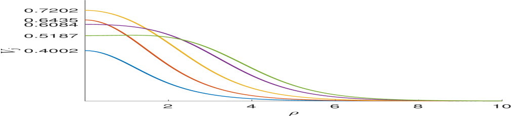
(a) $V_{j}$ with different $S$

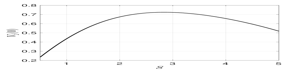
(b) Spot height versus $S$

(c) $\chi(S)$

Figure 1: Left panel: The core solution component $V_{j}(\rho)$, computed from (2.2), for $S=0.9\,,1.8\,,3.1\,,4.4$ and $5$ with corresponding spot heights $V_{j}(0)$ given approximately by $0.4002\,,0.6435\,,0.7202\,,0.6435\,,0.5187$, respectively. Middle panel: Spot height versus $S$, showing a monotone increase on $S<S^{\star}\approx 2.83$ and a unique spot height for each $S>0$. Right panel: $\chi$ versus $S$.

In Fig. 1 we plot the numerical solution $V_{j0}(\rho)$ to the core problem (2.2) for several source strengths. We show that there is a unique spot height $V_{j}(0)$ and a unique $\chi$ for each source strength.

To derive the outer problem for $u$, we integrate the equation for $U_{j0}$ in (2.2a) over $0<\rho<\infty$ to obtain the identity

$$S_{j}=\int_{0}^{\infty}U_{j0}V_{j0}^{2}\,\rho\,d\rho.$$ (2.4)

Then, in the limit $\varepsilon\to 0$, we use (2.4) to obtain, in the sense of distributions, that

$$\varepsilon^{-2}uv^{2}\to\sum\limits_{i=1}^{N}\left(\int_{\mathbb{R}^{2}}(D^{-1/2}U_{i0})(D^{1/2}V_{i0})^{2}d\mathbf{y}\right)\delta(\mathbf{x}-\mathbf{x}_{i})=2\pi\sqrt{D}\sum\limits_{i=1}^{N}S_{i}\,\delta(\mathbf{x}-\mathbf{x}_{i})\,.$$ (2.5)

By using this distributional limit in (1.1), we obtain that the outer problem, defined away from the spots, is

$$\Delta u+\frac{a}{D}-\frac{2\pi}{\sqrt{D}}\sum\limits_{i=1}^{N}S_{i}\,\delta(\mathbf{x}-\mathbf{x}_{i})=0\quad\mbox{in}\quad\Omega\,,\qquad\partial_{n}u=0\quad\mbox{on}\quad\partial\Omega\,.$$ (2.6)

By integrating (2.6) over $\Omega$ and using the divergence theorem, we get

$$\sum\limits_{i=1}^{N}S_{i}=\frac{a|\Omega|}{2\pi\sqrt{D}}\equiv p_{a}\,,$$ (2.7)

where $|\Omega|$ denotes the area of $\Omega$. The solution to (2.6) is represented as

$$u(\mathbf{x})=-\frac{2\pi}{\sqrt{D}}\sum\limits_{i=1}^{N}S_{i}\,G(\mathbf{x};\mathbf{x}_{i})+\bar{u}\,,$$ (2.8)

where $\bar{u}$ is an undetermined additive constant and $G(\mathbf{x};\mathbf{z})$ is the unique Neumann Green’s function satisfying

$$\Delta G=\frac{1}{|\Omega|}-\delta(\mathbf{x}-\mathbf{z})\quad\mbox{in}\quad\Omega\,,\quad\partial_{n}G=0\quad\mbox{on}\quad\partial\Omega\,;\qquad\int_{\Omega}G(\mathbf{x};\mathbf{z})\,d\mathbf{x}=0\,,$$ (2.9)

$$G\sim-\frac{1}{2\pi}\log|\mathbf{x}-\mathbf{z}|+R(\mathbf{z};\mathbf{z})+\nabla_{\mathbf{x}}R(\mathbf{x},\mathbf{z})|_{\mathbf{x}=\mathbf{z}}\cdot(\mathbf{x}-\mathbf{z})+{\mathcal{O}}(|\mathbf{x}-\mathbf{z}|^{2})\,,\quad\mbox{as}\quad\mathbf{x}\to\mathbf{z}\,,$$

where $R(\mathbf{z};\mathbf{z})$ is called the regular part of $G$.

To determine a nonlinear algebraic system for the source strengths, and a DAE system for slow spot dynamics, we must match the near-field behavior as $\mathbf{x}\to\mathbf{x}_{j}$ of the outer solution (2.8) to the far-field behavior of the two-term inner solution, which is given from (2.2b) and (2.1) by

$$u\sim\frac{1}{\sqrt{D}}\left(S_{j}\log\rho+\chi(S_{j})+\varepsilon U_{j1}+\cdots\right)=\frac{1}{\sqrt{D}}\left(S_{j}\log|\mathbf{x}-\mathbf{x}_{j}|+\frac{S_{j}}{\nu}+\chi(S_{j})\right)+\frac{\varepsilon U_{j1}}{\sqrt{D}}+\cdots\,,$$ (2.10)

as $\rho=\varepsilon^{-1}|\mathbf{x}-\mathbf{x}_{j}|\to\infty$, where we have defined $\nu\equiv{-1/\log\varepsilon}$. Then, by Taylor-expanding (2.8) as $\mathbf{x}\to\mathbf{x}_{j}$, and replacing $\mathbf{x}-\mathbf{x}_{j}=\varepsilon\mathbf{y}$, we obtain after some algebra that

$$u\sim\frac{S_{j}}{\sqrt{D}}\log|\mathbf{x}-\mathbf{x}_{j}|-\frac{2\pi}{\sqrt{D}}\left(S_{j}R_{j,j}+\sum\limits_{i\neq j}^{N}S_{i}G_{j,i}\right)+\bar{u}-\frac{\varepsilon}{\sqrt{D}}\,(\boldsymbol{\beta}_{j}\cdot\mathbf{y})+\cdots\,,$$ (2.11)

where $\boldsymbol{\beta}_{j}$ is defined by

$$\boldsymbol{\beta}_{j}\equiv 2\pi\left(S_{j}\nabla_{\mathbf{x}}R_{j,j}+\sum\limits_{i\neq j}^{N}S_{i}\nabla_{\mathbf{x}}G_{j,i}\right)\,.$$ (2.12)

Here we have labeled $R_{j,j}\equiv R(\mathbf{x}_{j};\mathbf{x}_{j})$, $G_{j,i}\equiv G(\mathbf{x}_{j};\mathbf{x}_{i})$, $\nabla_{\mathbf{x}}R_{j,j}\equiv\nabla_{\mathbf{x}}R(\mathbf{x};\mathbf{x}_{j})|_{\mathbf{x}=\mathbf{x}_{j}}$, and $\nabla_{\mathbf{x}}G_{j,i}\equiv\nabla_{\mathbf{x}}G(\mathbf{x};\mathbf{x}_{i})|_{\mathbf{x}=\mathbf{x}_{j}}$.

By comparing the leading terms in (2.10) and (2.11), and recalling (2.7), we obtain in matrix form that

$$\mathbf{s}+2\pi\nu\,\mathcal{G}\,\mathbf{s}+\nu\bm{\chi}=\nu\bar{u}\sqrt{D}\,\mathbf{e}\,,\qquad\mathbf{e}^{T}\mathbf{s}=p_{a}\equiv\frac{a|\Omega|}{2\pi\sqrt{D}}\,,$$ (2.13a)

where we have defined $$\mathbf{s} \bm{\chi} \mathbf{e} \mathcal{G}\in\mathbb{R}^{N\times N} \mathbf{x}_{1},\ldots,\mathbf{x}_{N}$$, , , and the Neumann Green’s matrix for by

$$\mathbf{s}=(S_{1},\ldots,S_{N})^{T}\,,\qquad\bm{\chi}\equiv(\chi(S_{1}),\ldots,\chi(S_{N}))^{T}\,,\qquad\mathbf{e}\equiv(1,\ldots,1)^{T}\in\mathbb{R}^{N}\,,\qquad(\mathcal{G})_{i\,j}=\begin{cases}R_{j,j}\quad\text{if }i=j\,,\\ G_{i,j}\quad\text{if }i\neq j\,.\end{cases}$$ (2.13b)

By left-multiplying (2.13a) by $\mathbf{e}^{T}$, and by using $\mathbf{e}^{T}\mathbf{s}=p_{a}$, we can isolate $\bar{u}$. Then, by substituting $\bar{u}$ back into (2.13a), we can decouple (2.13a) to obtain that $\mathbf{s}$ satisfies the nonlinear algebraic system (NAS)

$$\mathbf{s}+2\pi\nu\,(\mathcal{I}-\mathcal{E})\,\mathcal{G}\mathbf{s}+\nu\,(\mathcal{I}-\mathcal{E})\,\bm{\chi}=\frac{p_{a}}{N}\mathbf{e}\,,\qquad\mbox{with}\qquad\bar{u}=\frac{p_{a}+2\pi\nu\,\mathbf{e}^{T}\mathcal{G}\,\mathbf{s}+\nu\,\mathbf{e}^{T}\bm{\chi}}{\nu\sqrt{D}N}\,.$$ (2.14)

Here $\mathcal{E}\equiv N^{-1}\mathbf{e}\mathbf{e}^{T}\in\mathbb{R}^{N\times N}$ and $\mathcal{I}\in\mathbb{R}^{N\times N}$ is the identity matrix.

To determine the slow dynamics, we proceed to next order and match the $\mathcal{O}(\varepsilon)$ terms in (2.10) and (2.11). This yields that the far-field behavior for the solution $U_{j1}$ to (2.3) is

$$U_{j1}\sim-\boldsymbol{\beta}_{j}\cdot\mathbf{y}\,,\quad\mbox{as}\quad\rho=|\mathbf{y}|\to\infty\,,$$ (2.15)

where $\boldsymbol{\beta}_{j}$ is defined in (2.12). The ODE system for the spot locations is obtained by imposing a solvability condition on the solution to (2.3) with far-field behavior (2.15). By differentiating the core problem (2.2) with respect to $y_{1}$ and $y_{2}$, it follows that the homogeneous problem $\Delta_{\mathbf{y}}\mathbf{\Phi}+M_{j}\mathbf{\Phi}=\mathbf{0}$ has two non-trivial solutions. As such, there are two solutions to the corresponding homogeneous adjoint problem $\Delta_{\mathbf{y}}\mathbf{\Psi}+M_{j}^{T}\mathbf{\Psi}=\mathbf{0}$. These two solutions have the form

$$\mathbf{\Psi}_{c}=\mathbf{P}(\rho)\cos\phi\,,\qquad\mathbf{\Psi}_{s}=\mathbf{P}(\rho)\sin\phi\,,$$ (2.16)

where $\mathbf{P}(\rho)\equiv\left(P_{1}(\rho),P_{2}(\rho)\right)^{T}$ is the normalized nontrivial solution to

$$\Delta_{\rho}\mathbf{P}-\frac{1}{\rho^{2}}\,\mathbf{P}+M_{j}^{T}\mathbf{P}=\mathbf{0}\,,\quad\mbox{with}\quad\mathbf{P}\sim\begin{pmatrix}0\\ {1/\rho}\end{pmatrix}\quad\mbox{as}\quad\rho\to\infty\,.$$ (2.17)

In [17] the solvability condition is obtained by multiplying (2.3a) by $\mathbf{\Psi}_{c}$ and $\mathbf{\Psi}_{s}$ and applying Green’s second identity on a sufficiently large circle where the far-field conditions (2.15) and (2.17) are imposed. This yields the following ODE system for $\mathbf{x}_{j}(\sigma)$, for $j=1,\ldots,N$, with $\sigma=\varepsilon^{2}t$, that characterize the slow spot dynamics:

$$\frac{d\mathbf{x}_{j}}{d\sigma}=-\gamma(S_{j})\,\boldsymbol{\beta}_{j}\,,\qquad\gamma(S_{j})\equiv-\frac{2}{\int_{0}^{\infty}P_{1}V_{j0}^{\prime}\,\rho\,d\rho}\,.$$ (2.18)

Here $\boldsymbol{\beta}_{j}$ is defined in (2.12), while $S_{1},\ldots,S_{N}$ satisfies the NAS (2.14). The plot in Fig. 3 of [17] of the numerically computed $\gamma(S_{j})$ shows that $\gamma(S_{j})>0$.

2.2 Linear stability analysis

The slow spot dynamics (2.18) is valid only when the quasi-equilibrium solution is linearly stable on ${\mathcal{O}}(1)$ time-scales. In this subsection we analyze the linear stability of the quasi-equilibrium solution, denoted by $v=v_{e}$ and $u=u_{e}$. To do so, we introduce the perturbation $v=v_{e}+e^{\lambda t}\phi$ and $u=u_{e}+e^{\lambda t}\eta$ into (1.1), and upon linearizing we obtain

$$\varepsilon^{2}\Delta\phi-\phi+2u_{e}v_{e}\phi+v_{e}^{2}\eta=\lambda\phi\,,\qquad D\Delta\eta+a-\varepsilon^{-2}\left(2u_{e}v_{e}\phi+v_{e}^{2}\eta\right)=\tau\lambda\eta\,,\quad\mbox{in}\quad\Omega\,,$$ (2.19)

with $\partial_{n}\phi=\partial_{n}\eta=0$ on $\partial\Omega$.

In the inner region near the $j^{\text{th}}$ spot we have to leading order that $v_{e}\sim\sqrt{D}\,V_{j0}(\rho)$ and $u_{e}\sim U_{j0}(\rho)/\sqrt{D}$, where $\rho=\varepsilon^{-1}|\mathbf{x}-\mathbf{x}_{j}|$, with $V_{j0}$ and $U_{j0}$ satisfying the core problem (2.2). By letting $\phi\sim e^{im\theta}\Phi_{j}(\rho)$ and $\eta\sim e^{im\theta}N_{j}(\rho)/D$, for the integer angular mode $m\geq 0$, we obtain the leading order inner eigenvalue problem

$$\Delta_{\rho}\Phi_{j}-\frac{m^{2}}{\rho^{2}}\Phi_{j}-\Phi_{j}+2\,U_{j0}V_{j0}\Phi_{j}+V_{j0}^{2}N_{j}=\lambda\Phi_{j}\,,\qquad\Delta_{\rho}N_{j}-\frac{m^{2}}{\rho^{2}}N_{j}-2U_{j0}V_{j0}\Phi_{j}-V_{j0}^{2}N_{j}=0\,.$$ (2.20)

We first consider non-radially symmetric perturbations for which $m>0$. The case $m=1$ corresponds, trivially, to the translation mode $(\Phi_{j},N_{j})=(U_{j0}^{\prime},V_{j0}^{\prime})$ with $\lambda=0$. For angular modes with $m\geq 2$, we impose $\Phi_{j}\to 0$ exponentially as $\rho\to 0$. In addition, owing to the ${m^{2}N_{j}/\rho^{2}}$ term in (2.20), we impose the far-field decay condition $N_{j}\sim\mathcal{O}(\rho^{-m})$ as $\rho\to\infty$. The eigenvalue $\lambda_{\text{max}}$ in (2.20) with the largest real part has been numerically calculated in [17] for a range of $S_{j}$. For each $m\geq 2$, it was found that $\lambda_{\text{max}}$ is real and negative (positive) when $S_{j}<\Sigma_{m}$ ($S_{j}>\Sigma_{m}$) (see Fig. 4 of [17]). Moreover, as shown numerically in [17], the ordering principle $\Sigma_{2}<\Sigma_{3}<\ldots$ holds for the stability thresholds for non-radially symmetric perturbations. As such, the mode $m=2$, referred as to the peanut-splitting mode, is the first to lose stability when $S_{j}$ is increased. The critical threshold for this mode is $\Sigma_{2}\approx 4.302$. In [46] it was shown that this symmetry-breaking bifurcation is subcritical and, for a steady-state spot, it triggers a nonlinear spot self-replication process.

In contrast to the local analysis of instabilities associated with non-radially symmetric perturbations, the eigenvalue problem for radially symmetric perturbations with $m=0$ is derived by globally coupling local problems near each spot. To derive this globally coupled eigenvalue problem (GCEP), we set $m=0$ in (2.20) and impose that $N_{j}\sim c_{j}\log\rho$ as $\rho\to\infty$, where $c_{j}$ is an unknown constant. We then write

$$\Phi_{j}=c_{j}\tilde{\Phi}_{j}\,,\qquad N_{j}=c_{j}\tilde{N}_{j}\,,$$ (2.21)

so as to obtain from (2.20) that

$$\Delta_{\rho}\tilde{\Phi}_{j}- \tilde{\Phi}_{j}+2\,U_{j0}V_{j0}\,\tilde{\Phi}_{j}+V_{j0}^{2}\,\tilde{N}_{j}=\lambda\tilde{\Phi}_{j}\,,\qquad\Delta_{\rho}\tilde{N}_{j}-2\,U_{j0}V_{j0}\,\tilde{\Phi}_{j}-V_{j0}^{2}\,\tilde{N}_{j}=0\,,\quad\rho>0\,,$$ (2.22a)

$$\tilde{\Phi}_{j}^{\prime}(0)=\tilde{N}_{j}^{\prime}(0)=0\,;\qquad\tilde{\Phi}_{j}\to 0\,,\quad\tilde{N}_{j}\sim\log\rho+\tilde{B}(S_{j};\lambda)+o(1)\,,\quad\mbox{as}\quad\rho\to\infty\,,$$ (2.22b)

where $\tilde{B}(S_{j};\lambda)$ must be calculated numerically from (2.22). However, by differentiating the core problem (2.2) with respect to $S_{j}$, we observe that $\partial_{S}V_{j0}$ and $\partial_{S}U_{j0}$ satisfy (2.22) when $\lambda=0$. As a result, we have the identity that $\tilde{B}(S_{j};0)=\chi^{\prime}(S_{j})$.

By integrating the $\tilde{N}_{j}$ equation in (2.22), and using (2.21), we obtain the identity

$$c_{j}=\int_{0}^{\infty}\left(2U_{j0}V_{j0}\Phi_{j}+V_{j0}^{2}N_{j}\right)\rho\,d\rho\,.$$ (2.23)

Then, in the limit $\varepsilon\to 0$, we use (2.23) to derive, in the sense of distributions, that

$$\varepsilon^{-2}\left(2u_{e}v_{e}\phi+v_{e}^{2}\eta\right)\to 2\pi\sum\limits_{i=1}^{N}c_{i}\,\delta(\mathbf{x}-\mathbf{x}_{i})\,.$$ (2.24)

We use (2.24), together with the asymptotic matching condition $\eta\sim{c_{j}\tilde{N_{j}}/D}$, where $\tilde{N}_{j}$ has the far-field behavior as $\rho\to\infty$ in (2.22), to obtain the following outer problem for $\eta$, defined away from the spots:

$$\Delta\eta-\frac{\tau\lambda}{D}\eta =\frac{2\pi}{D}\sum\limits^{N}_{i=1}c_{i}\delta(\mathbf{x}-\mathbf{x}_{i})\quad\mbox{in}\quad\Omega\,,\qquad\partial_{n}\eta=0\quad\mbox{in}\quad\partial\Omega$$ (2.25a)

$$\eta \sim\frac{c_{j}}{D}\left[\log|\mathbf{x}-\mathbf{x}_{j}|+\frac{1}{\nu}+\tilde{B}(S_{j};\lambda)\right]\,,\quad\mbox{as}\quad\mathbf{x}\to\mathbf{x}_{j}\,,\qquad\mbox{for}\quad j=1,\ldots,N\,.$$ (2.25b)

For $\lambda\neq 0$, we represent the solution to (2.25a) as

$$\eta=-\frac{2\pi}{D}\sum\limits_{i=1}^{N}c_{i}\,G_{\lambda}(\mathbf{x};\mathbf{x}_{i})\,,$$ (2.26)

where $G_{\lambda}(\mathbf{x},\mathbf{z})$ is the eigenvalue-dependent Green’s function satisfying

$$\Delta G_{\lambda}-\frac{\tau\lambda}{D}G_{\lambda}=-\delta(\mathbf{x}-\mathbf{z})\quad\mbox{in}\quad\Omega\,,\qquad\partial_{n}G_{\lambda}=0\quad\mbox{on}\quad\partial\Omega\,,$$ (2.27a)

$$G_{\lambda}\sim-\frac{1}{2\pi}\log|\mathbf{x}-\mathbf{z}|+R_{\lambda}(\mathbf{z};\mathbf{z})+o(1)\quad\mbox{as}\quad\mathbf{x}\to\mathbf{z}\,.$$ (2.27b)

By Taylor-expanding $\eta$ in (2.26) as $\mathbf{x}\to\mathbf{x}_{j}$, and then equating the resulting expression with (2.25b), we conclude that

$$c_{j}+2\pi\nu\left(c_{j}R_{\lambda_{j,j}}+\sum\limits_{i\neq j}^{N}c_{i}\,G_{\lambda{j,i}}\right)+\nu\,c_{j}\tilde{B}(S_{j};\lambda)=0\,,\qquad j=1\,,\ldots,N\,,$$ (2.28)

where $R_{\lambda_{j,j}}\equiv R_{\lambda}(\mathbf{x}_{j};\mathbf{x}_{j})$ and $G_{\lambda{j,i}}\equiv G_{\lambda}(\mathbf{x}_{j};\mathbf{x}_{i})$. In matrix form, and with $\mathbf{c}\equiv(c_{1},\ldots,c_{N})^{T}$, (2.28) is equivalent to

$$\mathcal{M}(\lambda)\mathbf{c}=\mathbf{0}\,,\qquad\mbox{where}\qquad\mathcal{M}(\lambda)\equiv\mathcal{I}+2\pi\nu\mathcal{G}_{\lambda}+\nu\tilde{\mathcal{B}}\,.$$ (2.29a)

Here $$\mathcal{I}\in\mathbb{R}^{N\times N} \mathcal{G}_{\lambda} \tilde{\mathcal{B}}$$ is the identity matrix, while the symmetric Green’s matrix and diagonal matrix are defined by

$$\big{(}\mathcal{G}_{\lambda}\big{)}_{ij}\equiv\begin{cases}R_{\lambda_{j,j}}&\quad\mbox{if }i=j\,,\\ G_{\lambda{i,j}}&\quad\mbox{if }i\neq j\,,\end{cases}\qquad\big{(}\tilde{\mathcal{B}}\big{)}_{ij}=\begin{cases}\tilde{B}(S_{j};\lambda)&\quad\mbox{if }i=j\,,\\ 0&\quad\mbox{if }i\neq j\,.\end{cases}$$ (2.29b)

The homogeneous matrix system (2.29a) for $$\mathbf{c}$$, referred to as the GCEP, has a nontrivial solution if and only if

$$\det\mathcal{M}(\lambda)=0\,.$$ (2.29c)

A discrete root $\lambda$ to (2.29c) for which $\mbox{Re}(\lambda)>0$ corresponds to a locally radially symmetric instability near the spots, while the corresponding eigenvector $\mathbf{c}$ characterizes the small-scale perturbation of the spot amplitudes.

In this way, the linear stability properties associated with locally radially symmetric perturbations near the spots is reduced to the problem of determining the number ${\mathcal{N}}$ of roots of $\det\mathcal{M}(\lambda)=0$ in the right-half $\mbox{Re}(\lambda)>0$ of the spectral plane. To do so, we formulate and numerically implement a winding number procedure over the counterclockwise contour ${\mathcal{C}}_{\zeta}$ that consists of the semi-circle $|\lambda|=\zeta>0$, for $-\pi/2\leq\mbox{arg}\lambda\leq\pi/2$, and the imaginary segment $\{\lambda=i\lambda_{I}:-\zeta\leq\lambda_{I}\leq\zeta\}$. However, since $\mathcal{M}(\lambda)$ is undefined at $\lambda=0$, we need to first find the behavior of $\det\mathcal{M}(\lambda)$ as $\lambda\to 0$ so as to remove this singularity. To do so, we let $\lambda\to 0$ in (2.27) and readily calculate that

$$\mathcal{G}_{\lambda}=\frac{D}{|\Omega|\tau\lambda}\mathbf{e}\mathbf{e}^{T}+\mathcal{Q}\,,\qquad\mbox{where}\qquad\mathcal{Q}\equiv\mathcal{G}+\mathcal{O}(\tau\lambda)\quad\mbox{as}\quad\lambda\to 0\,.$$ (2.30)

Here $\mathcal{G}$ is the Neumann Green’s matrix and $\mathbf{e}\equiv(1,\ldots,1)^{T}$. Since $\mathbf{e}\mathbf{e}^{T}$ is a rank one matrix, we substitute (2.30) into (2.29a) for $\mathcal{M}$ and, by using the well-known matrix determinant lemma, we obtain

$$\det\mathcal{M}(\lambda)=\det\left(\mathcal{I}+2\pi\nu\mathcal{Q}+\nu\tilde{\mathcal{B}}\right)+\frac{2\pi\nu D}{|\Omega|\tau\lambda}\left[\mathbf{e}^{T}\mathrm{adj}\left(\mathcal{I}+2\pi\nu\mathcal{Q}+\nu\tilde{\mathcal{B}}\right)\mathbf{e}\right]\,,$$ (2.31)

where $\mathrm{adj}(\mathcal{A})$ denotes the adjugate of a matrix $\mathcal{A}$. From (2.31) it follows that $\det\mathcal{M}(\lambda)$ has a simple pole at $\lambda=0$. As a result, it is convenient to introduce the function ${\mathcal{T}}(\lambda)$ defined by ${\mathcal{T}}(\lambda)\equiv\lambda\det\mathcal{M}(\lambda)$, which has a removable singularity at $\lambda=0$ and has the same number ${\mathcal{N}}$ of zeroes in $\mbox{Re}(\lambda)>0$ as does $\det\mathcal{M}(\lambda)$. The argument principle for ${\mathcal{T}}$ yields that

$${\mathcal{N}}={\mathcal{P}}+\frac{1}{2\pi}\lim_{\zeta\to\infty}\left[\mbox{arg}{\mathcal{T}}(\lambda)\right]_{{\mathcal{C}}_{\zeta}}\,,\qquad\mbox{where}\qquad{\mathcal{T}}(\lambda)\equiv\lambda\det\mathcal{M}(\lambda)\,.$$ (2.32)

Here ${\mathcal{P}}$ is the number of poles of ${\mathcal{T}}(\lambda)$ in $\mbox{Re}(\lambda)>0$. Since ${\mathcal{G}}_{\lambda}$ is analytic in $\mbox{Re}(\lambda)>0$, any such pole can only arise from the diagonal matrix $\tilde{\mathcal{B}}$ as defined by (2.29b). However, from a numerical computation of the local problem (2.22), we find that $\tilde{\mathcal{B}}$ is analytic in $\mbox{Re}(\lambda)>0$ and so ${\mathcal{P}}=0$ in (2.32). To determine ${\mathcal{N}}$ in the examples below, the change $\left[\mbox{arg}{\mathcal{T}}(\lambda)\right]_{{\mathcal{C}}_{\zeta}}$ in the argument of ${\mathcal{T}}$ over the contour ${\mathcal{C}}_{\zeta}$ is computed numerically.

Next, we study zero-eigenvalue crossings. Since $\tilde{B}(S_{j};0)=\chi^{\prime}(S_{j})$, the outer problem (2.25a) when $\lambda=0$ becomes

$$\Delta\eta =\frac{2\pi}{D}\sum\limits^{N}_{i=1}c_{i}\delta(\mathbf{x}-\mathbf{x}_{i})\quad\mbox{in}\quad\Omega\,,\qquad\partial_{n}\eta=0\quad\mbox{in}\quad\partial\Omega$$ (2.33a)

$$\eta \sim\frac{c_{j}}{D}\left[\log|\mathbf{x}-\mathbf{x}_{j}|+\frac{1}{\nu}+\chi^{\prime}(S_{j})\right]\,,\quad\mbox{as}\quad\mathbf{x}\to\mathbf{x}_{j}\,,\quad j=1,\ldots,N\,.$$ (2.33b)

From the divergence theorem we conclude that $\sum_{i=1}^{N}c_{i}=0$. With this constraint, we represent the solution to (2.33a) in terms of the Neumann Green’s function $G$ of (2.9) as

$$\eta=-\frac{2\pi}{D}\sum\limits_{i=1}^{N}c_{i}\,G(\mathbf{x};\mathbf{x}_{i})+\bar{\eta}\,,$$ (2.34)

where $\bar{\eta}$ is an additive constant to be determined. Then, we Taylor-expand (2.34) as $\mathbf{x}\to\mathbf{x}_{j}$ by recalling the local behavior of $G$ in (2.9). By equating the resulting expression with the required singularity condition (2.33b), we obtain a matrix system for $\mathbf{c}=(c_{1},\ldots,c_{N})^{T}$ and $\bar{\eta}$ of the form

$$(\mathcal{I}+2\pi\nu\,\mathcal{G}+\nu\tilde{\mathcal{B}}_{0})\mathbf{c}=\nu\,\bar{\eta}\,\mathbf{e}\,,\qquad\mathbf{e}^{T}\mathbf{c}=0\,,$$ (2.35)

where $\mathcal{G}$ is the Neumann Green’s matrix and where the diagonal matrix $\tilde{\mathcal{B}}_{0}$ is defined by

$$\left(\tilde{\mathcal{B}}_{0}\right)_{i\,j}=\begin{cases}\chi^{\prime}(S_{j})&\quad\mbox{if }i=j\,,\\ 0&\quad\mbox{if }i\neq j\,,\end{cases}\qquad\longrightarrow\qquad\tilde{\mathcal{B}}_{0}\equiv\mbox{diag}\left(\chi^{\prime}(S_{1}),\ldots,\chi^{\prime}(S_{N})\right)\,.$$ (2.36)

By left-multiplying (2.35) by $\mathbf{e}^{T}$, and using $\mathbf{e}^{T}\mathbf{c}=0$, we find that $\bar{\eta}=N^{-1}\left(2\pi\mathbf{e}^{T}\mathcal{G}\mathbf{c}+\mathbf{e}^{T}\tilde{\mathcal{B}}_{0}\mathbf{c}\right)$. By substituting this expression back into the first equation in (2.35) we derive that

$$\mathcal{M}_{0}\mathbf{c}=\mathbf{0}\,,\qquad\mbox{where}\qquad\mathcal{M}_{0}\equiv\mathcal{I}+2\pi\nu(\mathcal{I}-\mathcal{E})\mathcal{G}+\nu(\mathcal{I}-\mathcal{E})\tilde{\mathcal{B}}_{0}\,,$$ (2.37)

where $\mathcal{E}\equiv N^{-1}\mathbf{e}\mathbf{e}^{T}$. We conclude that a zero-eigenvalue crossing associated with locally radially symmetric perturbations near the spots occurs if and only if $\det\mathcal{M}_{0}=0$. Since the corresponding nontrivial eigenmode $\mathbf{c}$ satisfies $\mathbf{e}^{T}\mathbf{c}=0$, it is referred to as a competition mode as it locally preserves the sum of all the spot amplitudes.

Finally, we relate the zero-eigenvalue crossing condition $\det\mathcal{M}_{0}=0$ to the local solvability of the NAS (2.14). Suppose, for a particular fixed parameter set, that $\mathbf{s}=\mathbf{s}_{e}$ is a non-degenerate solution to the NAS (2.14) in the sense that the Jacobian matrix of the NAS is invertible at $\mathbf{s}=\mathbf{s}_{e}$. Upon introducing the perturbation $\mathbf{s}=\mathbf{s}_{e}+\mathbf{c}$ into (2.14) where $|\mathbf{c}|\ll 1$, we linearize the NAS to readily determine that this Jacobian matrix is in fact the GCEP matrix $\mathcal{M}_{0}$ of (2.37), in which $\tilde{\mathcal{B}}_{0}\equiv\mbox{diag}\left(\chi^{\prime}(S_{1e}),\ldots,\chi^{\prime}(S_{Ne})\right)$. As a result, if $\mathbf{s}_{e}$ is a non-degenerate solution to the NAS (2.14) we must have $\det\mathcal{M}_{0}\neq 0$, and so $\lambda=0$ is not an eigenvalue of the GCEP. Therefore, it is only at a bifurcation point of the NAS (2.14) where a zero-eigenvalue crossing of the GCEP can occur. This correspondence is summarized as

$$\det\mathcal{M}_{0}=0\qquad\Longleftrightarrow\qquad\mathbf{s}_{e}\mbox{ is at a bifurcation point of the NAS }\eqref{proto:source_system}\,.$$ (2.38)

2.3 An $N$-spot ring pattern

An $N$-spot ring pattern is a pattern of $N$ equally-spaced spots located on a ring of radius $r_{0}$, with $0<r_{0}<1$, that is concentric within the unit disk $\Omega$. For $j=1,\ldots,N$, the locations of the spots on the ring can be taken as

$$\mathbf{x}_{j}=r_{0}\,\mathbf{e}_{\theta_{j}}\,,\qquad\mathbf{e}_{\theta_{j}}\equiv\left(\cos\theta_{j}\,,\,\sin\theta_{j}\right)^{T}\,,\qquad\theta_{j}\equiv\frac{2\pi(j-1)}{N}\,,\quad\mbox{for}\quad j=1,\ldots,N\,.$$ (2.39)

For a ring pattern, the symmetric Neumann Green’s matrix $\mathcal{G}$ is also circulant, and so it has the eigenvector $\mathbf{e}=(1,\ldots,1)^{T}$. As a result, the NAS (2.14) admits a symmetric solution where the spots have the common source strength $S_{j}=S_{c}\equiv{p_{a}/N}$, for $j=1,\ldots,N$, where $p_{a}$ is given in (2.7).

As shown in Appendix A, with $\mathbf{x}_{j}=r_{0}(\sigma)\mathbf{e}_{\theta_{j}}$ the spot dynamics given in (2.18) can be reduced to the scalar ODE

$$\frac{dr_{0}}{d\sigma}=\gamma(S_{c})S_{c}\left(\frac{N-1}{2r_{0}}-\frac{Nr_{0}^{2N-1}}{1-r_{0}^{2N}}-Nr_{0}\right)\,,\qquad\mbox{with}\quad S_{c}=\frac{a|\Omega|}{2\pi N\sqrt{D}}\,,$$ (2.40)

for the ring radius, where $\sigma=\varepsilon^{2}t$. On $0<r_{0}<1$, this ODE (2.40) has a globally stable equilibrium point $r_{0e}$, given by the unique root to

$$\frac{N-1}{2N}-r_{0}^{2}=\frac{r_{0}^{2N}}{1-r_{0}^{2N}}\,.$$ (2.41)

From §2.2, the $N$-spot ring pattern is linear stable to locally non-radially symmetric perturbations near the spots only when $S_{c}<\Sigma_{2}\approx 4.302$, where $S_{c}={a|\Omega|/[2\pi N\sqrt{D}]}$ with $|\Omega|=\pi$. In terms of the feed rate $a$, this stability condition holds when $a<a_{f}\equiv 2\Sigma_{2}\sqrt{D}N\approx 8.6DN$.

Next, we study the linear stability associated with radially-symmetric perturbations near the spots. For a ring pattern, the GCEP (2.29a) becomes

$$\mathcal{M}\mathbf{c}=\mathbf{0}\,,\qquad\mbox{where}\qquad\mathcal{M}=(1+\nu\tilde{B}_{c})\mathcal{I}+2\pi\nu\,\mathcal{G}_{\lambda}\,.$$ (2.42)

Here $\tilde{B}_{c}\equiv\tilde{B}(S_{c};\lambda)$ is to be calculated from the inner problem (2.22) with $S_{j}=S_{c}$. Owing to the cyclic structure of the ring pattern, the symmetric Green’s matrix $\mathcal{G}_{\lambda}$ is also a circulant matrix and, as a result, it has the matrix spectrum (see Appendix B)

$$\mathcal{G}_{\lambda}\mathbf{e}=\omega_{1}\mathbf{e}\,,\qquad\mathcal{G}_{\lambda}\mathbf{q}_{j}=\omega_{j}\mathbf{q}_{j}\,,\quad j=2,\ldots,N\,;\qquad\mathbf{e}^{T}\mathbf{q}_{j}=0\,,\quad\mathbf{q}_{i}^{T}\mathbf{q}_{j}=0\,,\quad i\neq j\,,$$ (2.43)

where $\mathbf{q}_{j}$ for $j=2,\ldots,N$ are given in (B.1b). The matrix eigenvalues $\omega_{j}$ are given in terms of the first row of $\mathcal{G}_{\lambda}$ by (B.1b), while the entries in $\mathcal{G}_{\lambda}$ can be evaluated numerically from the infinite series result in (A.5) of Appendix A for the eigenvalue-dependent Green’s function of (2.27).

Since $\mathcal{M}$ in (2.42) represents an update to $\mathcal{G}_{\lambda}$ by a multiple of the identity matrix, the eigenspace of $\mathcal{M}$ is the same as $\mathcal{G}_{\lambda}$. As a result, we simply substitute $\mathbf{c}_{1}=\mathbf{e}$ and $\mathbf{c}_{j}=\mathbf{q}_{j}$ into (2.42) to obtain the root finding problems ${\mathcal{F}}_{j}=0$, which are defined in terms of $\omega_{j}$ in (2.43) by

$${\mathcal{F}}_{j}\equiv 1+\nu\tilde{B}(S_{c};\lambda)+2\pi\nu\,\omega_{j}\,,\qquad j=1,\ldots,N\,.$$ (2.44)

We refer to $\mathbf{c}_{1}=\mathbf{e}$ and $\mathbf{c}_{j}=\mathbf{q}_{j}$, for $j=2,\ldots,N$, as the synchronous mode and asynchronous modes, respectively.

2.3.1 Example: instabilities associated with a two-spot ring pattern

We begin by analyzing the zero-eigenvalue crossing in the GCEP for an $N$-spot ring pattern. The criterion (2.37) becomes

$$\mathcal{M}_{0}\mathbf{c}=\mathbf{0}\,,\qquad\mbox{where}\qquad\mathcal{M}_{0}=\left(1+\nu\chi^{\prime}(S_{c})\right)\mathcal{I}+2\pi\nu(\mathcal{I}-\mathcal{E})\mathcal{G}-\nu\chi^{\prime}(S_{c})\mathcal{E}\,.$$ (2.45)

The matrix $\mathcal{M}_{0}$ shares the same eigenspace as the symmetric and circulant matrix $\mathcal{G}$, and so has eigenvectors $\mathbf{e},\mathbf{q}_{2},\ldots,\mathbf{q}_{N}$ as in (2.43). Since $\mathcal{G}\mathbf{e}=\sigma_{1}\mathbf{e}$, we use $\mathcal{E}\mathbf{e}=\mathbf{e}$ to calculate $\mathcal{M}_{0}\mathbf{e}=\mathbf{e}$. Therefore, the synchronous mode $\mathbf{c}=\mathbf{e}$ can never be a nullvector for $\mathcal{M}_{0}$. In contrast, with $\mathbf{c}=\mathbf{q}_{j}$ for $j=2,\ldots,N$, we use $\mathcal{E}\mathbf{q}_{j}=0$ to obtain that $\mathcal{M}_{0}\mathbf{c}=\mathbf{0}$ if and only if

$$1+\nu\chi^{\prime}(S_{c})+2\pi\nu\sigma_{j}=0\,,\qquad\mbox{where}\qquad\mathcal{G}\mathbf{q}_{j}=\sigma_{j}\mathbf{q}_{j}\,,\quad j=2,\ldots,N\,.$$ (2.46)

From (2.38), $\det\mathcal{M}_{0}=0$ can only occur at a bifurcation point for the NAS (2.14).

As an example, we investigate competition instabilities for a two-spot equilibrium ring pattern in the unit disk with $\varepsilon=0.02$, $D=1$, and ring radius $r_{0}=0.4536$ determined from (2.41). Since $\mathbf{q}_{2}=(1,-1)^{T}$ is the only competition mode, we use $S_{c}={a/[2N\sqrt{D}]}={a/4}$ with $j=N=2$ to write (2.46) as a nonlinear algebraic equation in the feed rate $a$. This equation is solved numerically to obtain the competition threshold $a_{comp}\approx 4.45$. To interpret this bifurcation point, we determine asymmetric branches of two-spot ring patterns from the NAS (2.14) with $N=2$. Labeling $S_{1}$ and $S_{2}$ as the source strengths of the two spots, we set $S_{2}=p_{a}-S_{1}$ in (2.14) with $N=2$ to obtain a scalar nonlinear algebraic equation for $S_{1}$ given by

$$\left(1+2\pi\nu(R_{11}-G_{12})\right)S_{1}+\frac{\nu}{2}\left[\chi(S_{1})-\chi(p_{a}-S_{1})\right]=\frac{p_{a}}{2}\left(1+2\pi\nu(R_{11}-G_{12})\right)\,,\quad\mbox{where}\quad p_{a}\equiv\frac{a}{2}\,.$$ (2.47)

By solving (2.47) numerically, in Fig. 2(a) we show the bifurcation structure of $S_{1}$ versus $a$. The symmetric branch corresponds to the common source strength $S_{1}=S_{2}\equiv S_{c}={a/4}$. It undergoes a pitchfork bifurcation at $a=a_{\text{comp}}\approx 4.45$, for which from (2.38) a zero-eigenvalue crossing for the GCEP must occur. Moreover, asymmetric branches of quasi-equilibria with $S_{1}\neq S_{2}$ exist for $a>a_{\text{comp}}$. In the same figure, we superimpose PDE simulation data computed from (1.1) with a slowly decreasing feed rate $a=\max(4.7-0.005\,t\,,3.5)$. As the feed rate drops below $a_{\text{comp}}$, only one spot survives and there is a fast transition to the one-spot branch where $S_{1}={a/2}$ (dotted line in Fig. 2(a)).

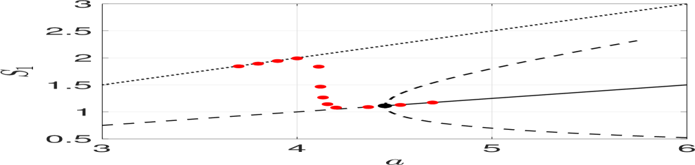
(a) Pitchfork bifurcation: two-spot ring pattern

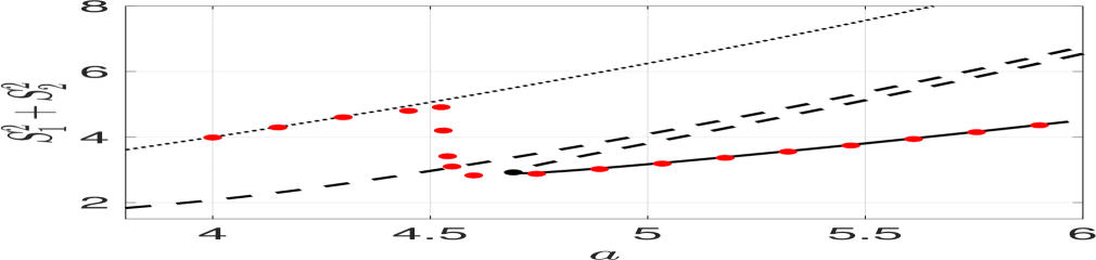
(b) Imperfect bifurcation: perturbed two-spot pattern

Figure 2: Left panel: Source strength $S_{1}$ versus $a$ for a two-spot equilibrium ring pattern with $\varepsilon=0.02$, $D=1$, and ring radius $r_{0}=0.4536$. The solid (dashed) portion in the pitchfork structure has zero (one) unstable eigenvalue for the GCEP (2.42). The red dots represent the $S_{1}$ data interpolated from the PDE simulation with slowly decreasing feed rate $a=\max(4.7-0.005\,t\,,3.5)$. We observe that $S_{1}$ jumps to the one-spot branch where $S_{1}={a/2}$ (dotted line). Right panel: Same parameters except that now spots are at $\mathbf{x}_{1}=(0.5,0)$ and $\mathbf{x}_{2}=(-0.6,0)$. The thick solid and dashed curves are the stable and unstable branches of two-spot quasi-equilibria. The source strength from PDE data (red dots) is obtained by mapping from the the spot height. As $a$ is swept with $a=\max(4,6-(\varepsilon/2)t)$ below the saddle-node point, only one spot survives. The sum of squares of the source strength jumps to the one-spot branch $S_{1}^{2}=a^{2}/4$ (dotted line).

To illustrate an imperfection sensitivity in the bifurcation structure of two-spot quasi-equilibria, we consider a two-spot pattern with spots located at $\mathbf{x}_{1}=(0.5,0)$ and $\mathbf{x}_{2}=(-0.6,0)$ in the unit disk with $\varepsilon=0.02$ and $D=1$. Through numerical continuation of the NAS (2.14) with bifurcation parameter $a$ using COCO [8], in Fig. 2(b) we observe two isolated branches of $S_{1}^{2}+S_{2}^{2}$, with one branch having a saddle-node bifurcation at $a\approx 4.609$, which must correspond to a zero-eigenvalue of the GCEP. The linear stability properties of these branches, as indicated in the caption of Fig. 2(b), was obtained from a numerical computation of the winding number in (2.32). From the results of a full PDE computation of (1.1) with a slowly decreasing feed-rate $a=\max(4,6-(\varepsilon/2)t)$ with $\varepsilon=0.02$, in Fig. 2(b) we show that as $a$ sweeps below the saddle-node point for two-spot quasi-equilibria, one spot gets annihilated while the remaining spot jumps to the stable one-spot branch.

Next, we illustrate how a pair of unstable eigenvalues emerge from a Hopf bifurcation as $\tau$ is increased. We consider a two-spot equilibrium ring pattern in the unit disk with $\varepsilon=0.02$ and $D=1$. The two spots are centered at $(\pm r_{0},0)$, where $r_{0}\approx 0.4536$ is the steady-state two-spot ring radius, as calculated from (2.41) when $N=2$. By varying the feed rate $a$, on the range $4.45\approx a_{\text{comp}}<a<a_{f}\approx 17.2$ (heavy solid curve in Fig. 2(a)), we use (2.44) to numerically compute the Hopf bifurcation thresholds for $\tau$ for the synchronous mode $(j=1)$ and the asynchronous mode $(j=2)$. This is done by using Newton’s method to solve for $(\lambda_{I}^{(j)},\tau_{H}^{(j)})$ in

$$\mbox{Re}\left[F_{j}(i\lambda_{I}^{(j)},\tau_{H}^{(j)})\right]=0\,,\qquad\mbox{Im}\left[F_{j}(i\lambda_{I}^{(j)},\tau_{H}^{(j)})\right]=0\,,\quad\mbox{for}\quad j=1\,,2\,.$$ (2.48)

The results for $\tau_{H}^{(j)}$ and $\lambda_{I}^{(j)}$ for $j=1,2$ versus the feed rate $a$ are shown in the left and right panels of Fig. 3, respectively. From this figure, we observe that the mode that synchronizes the temporal oscillations in the spot amplitudes is the first to go unstable as $\tau$ is increased. A numerical implementation of the winding number criterion in (2.32) yields that the two-spot ring pattern is linearly stable when $\tau<\min(\tau_{H}^{(1)},\tau_{H}^{(2)})$.

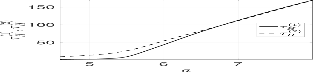
(a) Hopf bifurcation threshold for $\tau$

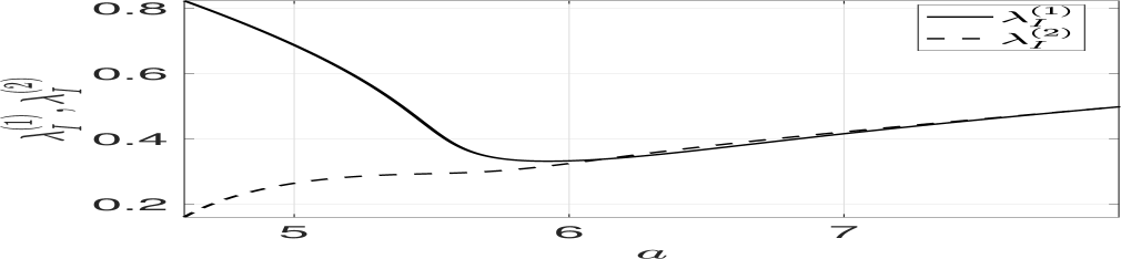
(b) Imaginary eigenvalue at the Hopf bifurcation

Figure 3: Left panel: The Hopf bifurcation value of $\tau$ for the synchronous $(j=1)$ and asynchronous mode $(j=2)$, as computed from (2.48), for the linearization of a two-spot ring steady-state solution with $\varepsilon=0.02$, $D=1$, and ring radius $r_{0}=0.4536$. The thresholds become almost indistinguishable as the feed rate $a$ is increased. Right panel: The corresponding imaginary eigenvalue for the two modes.

To confirm the Hopf bifurcation threshold, as calculated from (2.48), we compute full numerical solution to the PDE (1.1) for $\varepsilon=0.02$, $D=1$, using as an initial condition a two-spot ring pattern with ring radius $r_{0}=0.4536$. For $a=6$, we have $\tau_{H}^{(1)}\approx 43.56$ and $\tau_{H}^{(2)}\approx 54.28$ from (2.48). With the choice $\tau=54$, for which $\tau_{H}^{(1)}<\tau<\tau_{H}^{(2)}$, we predict from the GCEP that the amplitudes of the two spots will oscillate in phase. In the PDE simulation results of Fig. 4(a) we show that there are synchronous oscillations of the spot amplitudes, which eventually leads to the disappearance of both spots. By increasing the feed rate to $a=7.2$, we have $\tau_{H}^{(1)}\approx 124.56$ and $\tau_{H}^{(2)}\approx 123.11$ from (2.48). With the choice $\tau=137$, we predict that the two spots will be unstable to both synchronous and asynchronous perturbations in the spot amplitudes. In the PDE simulation results of Fig. 4(b) we show that, although initially the spot amplitudes oscillate synchronously. as time increases these oscillations become asynchronous, and eventually one of the two spots is annihilated.

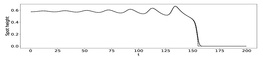
(a) $a=6$ and $\tau_{H}^{(1)}<\tau<\tau_{H}^{(2)}$.

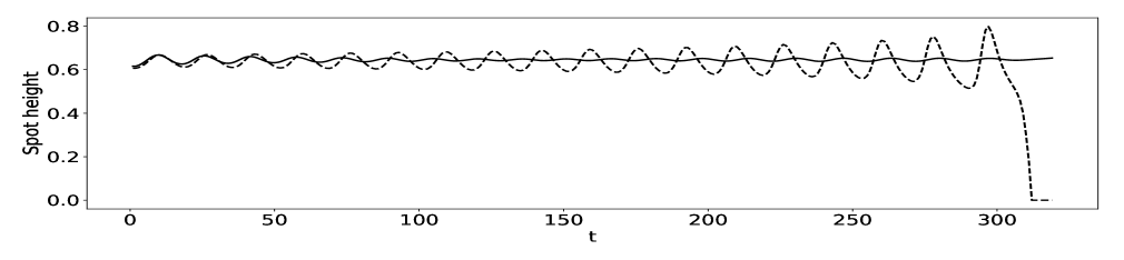
(b) $a=7.2$ and $\tau_{H}^{(2)}<\tau_{H}^{(1)}<\tau$.

Figure 4: PDE simulation results of (1.1) for the spot amplitudes versus time starting from a two-spot steady-state ring pattern with $\varepsilon=0.02$, $D=1$, and ring radius $r_{0}=0.4536$. Left panel: $a=6$ and $\tau=54$. Synchronous oscillations occur, leading to the annihilation of both spots. Right panel: $a=7.2$ and $\tau=137$. Eventually asynchronous spot amplitude oscillations occur, leading to the annihilation of only one spot.

3 A perforation of the domain as a localized defect

In this section we analyze how the existence, linear stability, and slow dynamics of quasi-equilibrium spot patterns are affected by removing a small circular hole of radius ${\mathcal{O}}(\varepsilon)$ from $\Omega$, given by

$$\Omega_{\varepsilon}=\big{\{}\mathbf{x}\in\Omega\,:\,|\mathbf{x}-\mathbf{x}_{0}|\leq C\varepsilon\,\big{\}}\,,$$

where $C>0$ is an $\mathcal{O}(1)$ parameter controlling the size of the hole. In the perforated domain, the Schnakenberg model is

$$v_{t} =\varepsilon^{2}\Delta v-v+uv^{2}\,,\qquad\tau u_{t}=D\Delta u+a-\frac{uv^{2}}{\varepsilon^{2}}\,,\quad\mbox{in}\quad\bar{\Omega}\equiv\Omega\setminus\Omega_{\varepsilon}\,,$$ (3.1a)

$$\partial_{n}v =\partial_{n}u=0\quad\mbox{on}\quad\partial\Omega\,;\qquad v=u=0\quad\mbox{on}\quad\partial\Omega_{\varepsilon}\,.$$ (3.1b)

The homogeneous Dirichlet boundary conditions on $\partial\Omega_{\varepsilon}$ models the leakage of the activator $v$ and the substrate $u$ through the boundary of the small hole.

3.1 Quasi-equilibrium $N$-spot pattern and slow dynamics

We begin by constructing a quasi-equilibrium $N$-spot pattern with spots located at $\mathbf{x}_{1},\ldots,\mathbf{x}_{N}$ in the perforated domain. We assume, initially, that this pattern is linearly stable on $\mathcal{O}(1)$ time intervals. In our analysis below, we assume that $|\mathbf{x}_{i}-\mathbf{x}_{j}|=\mathcal{O}(1)$ for $i\neq j$, and that $\mbox{dist}(\mathbf{x}_{i},\partial\Omega)=\mathcal{O}(1)$ and $\mbox{dist}(\mathbf{x}_{i},\partial\Omega_{\varepsilon})=\mathcal{O}(1)$ for $i=1,\ldots,N$.

Following the derivation in §2.1, the outer problem for the inhibitor field, defined away from the spots, is

$$\Delta u+\frac{a}{D}-\frac{2\pi}{\sqrt{D}}\sum\limits_{i=1}^{N}S_{i}\,\delta(\mathbf{x}-\mathbf{x}_{i})=0\quad\mbox{in}\quad\bar{\Omega}\,,\quad\partial_{n}u=0\quad\mbox{on}\quad\partial\Omega\,;\qquad u=0\quad\mbox{on}\quad\partial\Omega_{\varepsilon}\,,$$ (3.2)

where $S_{1},\ldots,S_{N}$ denote the spot source strengths. However, this outer problem is of singular perturbation type since $u$ must satisfy the extra conditon $u=0$ on $\partial\Omega_{\varepsilon}$. To proceed, we will use strong localized perturbation theory to replace the effect of the hole with a Dirac singularity. To do so, near the hole centered at $\mathbf{x}_{0}$ we introduce local coordinates $\mathbf{y}=\varepsilon^{-1}(\mathbf{x}-\mathbf{x}_{0})$ and $u\sim U_{0}(\mathbf{y})/\sqrt{D}$. From (3.2), we obtain to leading order that

$$\Delta_{\mathbf{y}}U_{0}=0\,,\quad|\mathbf{y}|\geq C\,;\qquad U_{0}=0\,,\quad\mbox{on}\quad|\mathbf{y}|=C\,,$$ (3.3)

which has the solution $U_{0}=S_{0}\log\left(|\mathbf{y}|/C\right)$, where $S_{0}$ is to be determined. This yields the matching condition

$$u\sim\frac{U_{0}}{\sqrt{D}}\sim\frac{S_{0}}{\sqrt{D}}\left(\log|\mathbf{x}-\mathbf{x}_{0}|+\frac{1}{\nu}-\log C\right)\,,\quad\mbox{as}\quad\mathbf{x}\to\mathbf{x}_{0}\,,$$ (3.4)

where $\nu={-1/\log\varepsilon}$. Owing to the identity

$$\int_{\partial\Omega_{\varepsilon}}-D\partial_{n}u|_{\partial\Omega_{\varepsilon}}\,ds\sim 2\pi S_{0}\sqrt{D}\,,$$ (3.5)

where $\partial_{n}$ denotes the outward normal derivative to $\bar{\Omega}$, the constant $S_{0}$ is proportional to the diffusive flux of inhibitor through the hole. The strength of this leakage term, mediated by $S_{0}$, is calculated below in a self-consistent way.

By superimposing the Dirac singularity $\dfrac{2\pi S_{0}}{\sqrt{D}}\,\delta(\mathbf{x}-\mathbf{x}_{0})$ on the outer problem to account for the logarithmic singularity in (3.4), we replace (3.2) with the modified outer problem

$$\Delta u+\frac{a}{D}-\frac{2\pi}{\sqrt{D}}\sum\limits_{i=0}^{N}S_{i}\,\delta(\mathbf{x}-\mathbf{x}_{i})=0\quad\mbox{in}\quad\Omega\,;\qquad\partial_{n}u=0\quad\mbox{on}\quad\partial\Omega\,,$$ (3.6)

which is defined at ${\mathcal{O}}(1)$ distances from the spot locations and from the center of the hole.

The solution to (3.6) is represented in terms of the Neumann Green’s function of (2.9) as

$$u(\mathbf{x})=-\frac{2\pi}{\sqrt{D}}\sum\limits_{i=0}^{N}S_{i}\,G(\mathbf{x};\mathbf{x}_{i})+\bar{u}\,,$$ (3.7)

where $\bar{u}$ is a constant to be determined. By applying the divergence theorem to (3.6) we get

$$\sum\limits_{i=0}^{N}S_{i}=\frac{a|\Omega|}{2\pi\sqrt{D}}\equiv p_{a}\,.$$ (3.8)

We let $\mathbf{x}\to\mathbf{x}_{0}$ in (3.7) in order to asymptotically match the local behavior of $u$ with the far-field behavior (3.4) for the solution near the hole. This matching yields the algebraic equation

$$S_{0}+2\pi\nu\left(S_{0}R_{0,0}+\sum\limits_{i=1}^{N}S_{i}\,G_{0,i}\right)-\nu S_{0}\log C=\nu\sqrt{D}\,\bar{u}\,,$$ (3.9)

where $R_{0,0}\equiv R(\mathbf{x}_{0};\mathbf{x}_{0})$ and $G_{0,i}\equiv G(\mathbf{x}_{0};\mathbf{x}_{i})$.

Next, we match the local behavior of the outer solution in (3.7) near each spot with the far-field behavior (2.10) of the corresponding inner solution. Letting $\mathbf{x}\to\mathbf{x}_{j}$ in (3.7) we obtain that

$$\begin{split}u&\sim\frac{S_{j}}{\sqrt{D}}\log|\mathbf{x}-\mathbf{x}_{j}|-\frac{2\pi}{\sqrt{D}}\left(S_{j}R_{j,j}+\sum\limits_{i\neq j}^{N}S_{i}\,G_{j,i}+S_{0}\,G_{j,0}\right)+\bar{u}\\ &\qquad-2\pi\left(S_{j}\nabla_{\mathbf{x}}R_{j,j}+\sum\limits_{i\neq j}^{N}S_{i}\nabla_{\mathbf{x}}G_{j,i}+S_{0}\nabla_{\mathbf{x}}G_{j,0}\right)\cdot(\mathbf{x}-\mathbf{x}_{j})+{\mathcal{O}}(|\mathbf{x}-\mathbf{x}_{j}|^{2})\,,\qquad j=1,\ldots,N\,.\end{split}$$ (3.10)

By matching the $\mathcal{O}(1)$ terms in (2.10) and (3.10), we obtain that

$$S_{j}+2\pi\nu\left(S_{j}R_{j,j}+\sum\limits_{i\neq j}^{N}S_{i}\,G_{j,i}+S_{0}\,G_{j,0}\right)+\nu\chi(S_{j})=\nu\sqrt{D}\bar{u}\,,\qquad j=1,\ldots,N\,.$$ (3.11)

We write the nonlinear algebraic system (3.8), (3.9), and (3.11) for $S_{0},\ldots,S_{N}$ and $\bar{u}$ in matrix form as

$$S_{0}=p_{a}-\mathbf{e}^{T}\mathbf{s}\,,\qquad\mathbf{s}+2\pi\nu\left(\mathcal{G}\mathbf{s}+S_{0}\mathbf{g}\right)+\nu\bm{\chi}=\left(\nu\sqrt{D}\bar{u}\right)\mathbf{e}\,,\qquad\theta S_{0}=\nu\sqrt{D}\bar{u}-2\pi\nu\mathbf{g}^{T}\mathbf{s}\,,$$ (3.12a)

where we have defined

$$\begin{split}&\mathbf{s}\equiv(S_{1},\ldots,S_{N})^{T}\,,\qquad\mathbf{g}\equiv(G_{0,1},\ldots,G_{0,N})^{T}\,,\qquad\mathbf{e}\equiv(1,\ldots,1)^{T}\in\mathbb{R}^{N}\,,\\ &\bm{\chi}\equiv(\chi(S_{1}),\ldots,\chi(S_{N}))^{T}\,,\qquad\theta\equiv 1+2\pi\nu R_{0,0}-\nu\log C\,.\end{split}$$ (3.12b)

Here $\mathcal{G}\in\mathbb{R}^{N\times N}$ is the Neumann Green’s matrix characterizing inter-spot interactions for spots centered at $\mathbf{x}_{1},\ldots,\mathbf{x}_{N}$. By eliminating $S_{0}$ between the first and third equations in (3.12a), we can solve for $\bar{u}$ as

$$\bar{u}=\frac{\theta p_{a}+\mathbf{s}^{T}(2\pi\nu\mathbf{g}-\theta\mathbf{e})}{\nu\sqrt{D}}\,.$$ (3.13)

By substituting (3.13) together with $S_{0}=p_{a}-\mathbf{e}^{T}\mathbf{s}$ into the middle equation of (3.12a) we obtain the following nonlinear algebraic system for the vector $\mathbf{s}$ of spot strengths:

$$\mathbf{s}+2\pi\nu\mathcal{G}\mathbf{s}+(\mathbf{e}^{T}\mathbf{s})\left(\theta\mathbf{e}-4\pi\nu\mathbf{g}\right)+\nu\bm{\chi}=p_{a}\left(\theta\mathbf{e}-2\pi\nu\mathbf{g}\right)\,.$$ (3.14)

Next, to derive the DAE system for slow spot dynamics, we match (2.10) with (3.10) for the $\mathcal{O}(\varepsilon)$ gradient terms. Denoting $\mathbf{y}=\varepsilon^{-1}(\mathbf{x}-\mathbf{x}_{j})$, and using $S_{0}=p_{a}-\mathbf{e}^{T}\mathbf{s}$, this yields the following far-field behavior for the correction $U_{j1}$ to the leading order core solution, as defined in (2.1):

$$U_{j1}\sim-\left(\boldsymbol{\beta}_{j}+2\pi S_{0}\nabla_{\mathbf{x}}G_{j,0}\right)\cdot\mathbf{y}=-\left[\boldsymbol{\beta}_{j}+2\pi\left(p_{a}-\sum\limits_{i=1}^{N}S_{i}\right)\nabla_{\mathbf{x}}G_{j,0}\right]\cdot\mathbf{y}\,,\quad\mbox{as}\quad|\mathbf{y}|\to\infty\,.$$ (3.15)

Here $\boldsymbol{\beta}_{j}$ is defined in (2.12). Following the derivation in §2.1, we conclude that the DAE system for slow spot dynamics is given by

$$\frac{d\mathbf{x}_{j}}{d\sigma}=-\gamma(S_{j})\left[\boldsymbol{\beta}_{j}+2\pi\left(p_{a}-\sum\limits_{i=1}^{N}S_{i}\right)\nabla_{\mathbf{x}}G_{j,0}\right]\,,\qquad j=1,\ldots,N\,,$$ (3.16)

where $\sigma=\varepsilon^{2}t$ and $\mathbf{s}\equiv(S_{1},\ldots,S_{N})^{T}$ satisfies the nonlinear algebraic system (3.14). Here $\gamma(S_{j})$ is defined in (2.18).

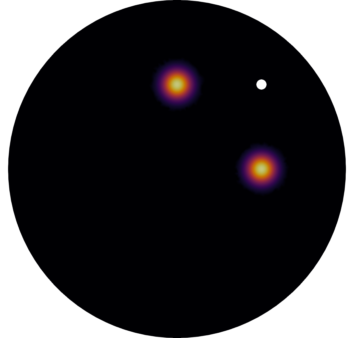
(a) $t=0$

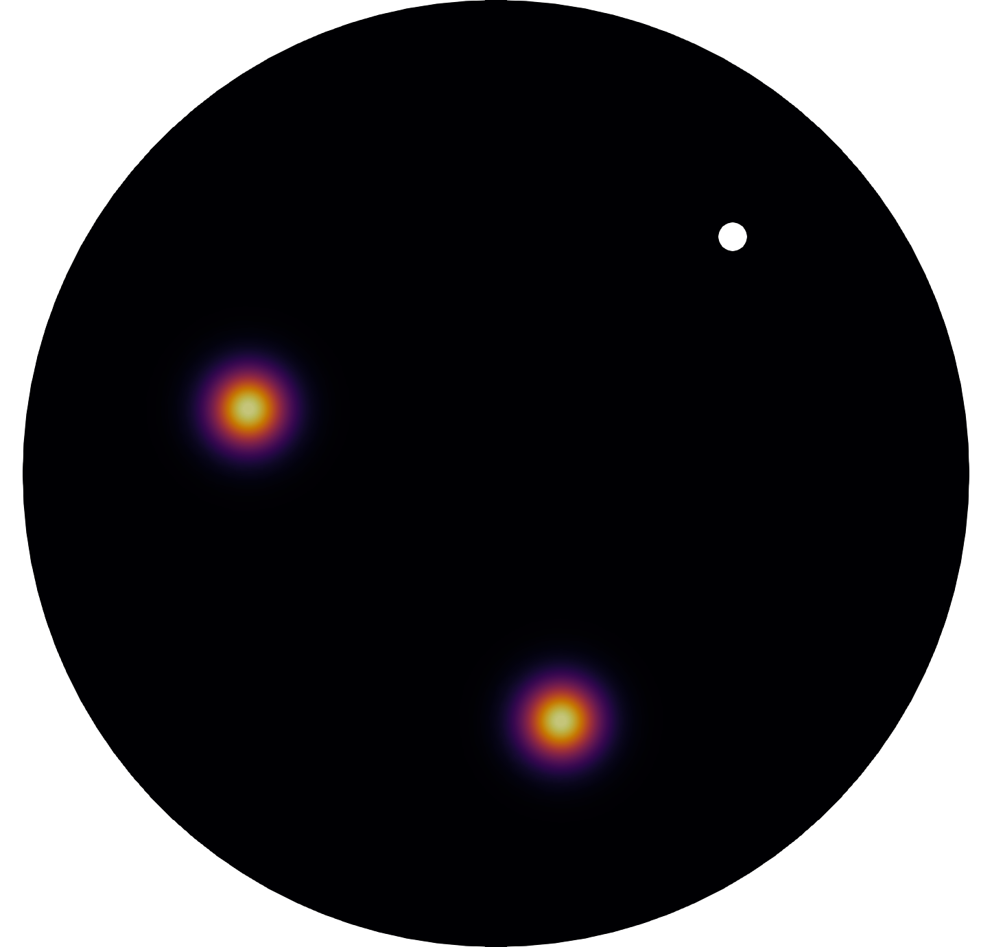
(b) $t=999$

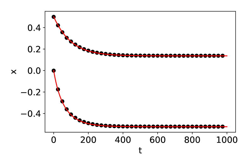
(c) $x$-coordinate of spots

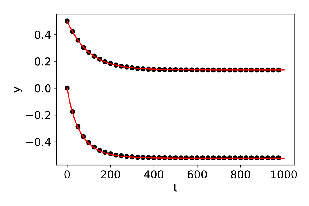
(d) $y$-coordinate of spots

Figure 5: For $\varepsilon=0.03,\,D=\tau=1,\,a=16$ and a hole at $\mathbf{x}_{0}=(0.5,0.5)$ with radius $\varepsilon$ ($C=1$), two spots initially located at $(0.5,0)$ and $(0,0.5)$, respectively, share the same source strength $S\approx 3.0599$. In (a) and (b), we show the numerical PDE solution of $v$ at $t=0$ and $t=999$, respectively. In (c) and (d), we show the very close agreement of spot trajectories obtained by the PDE simulation (black dots) and the DAE (3.16) and (3.14) (red solid line).

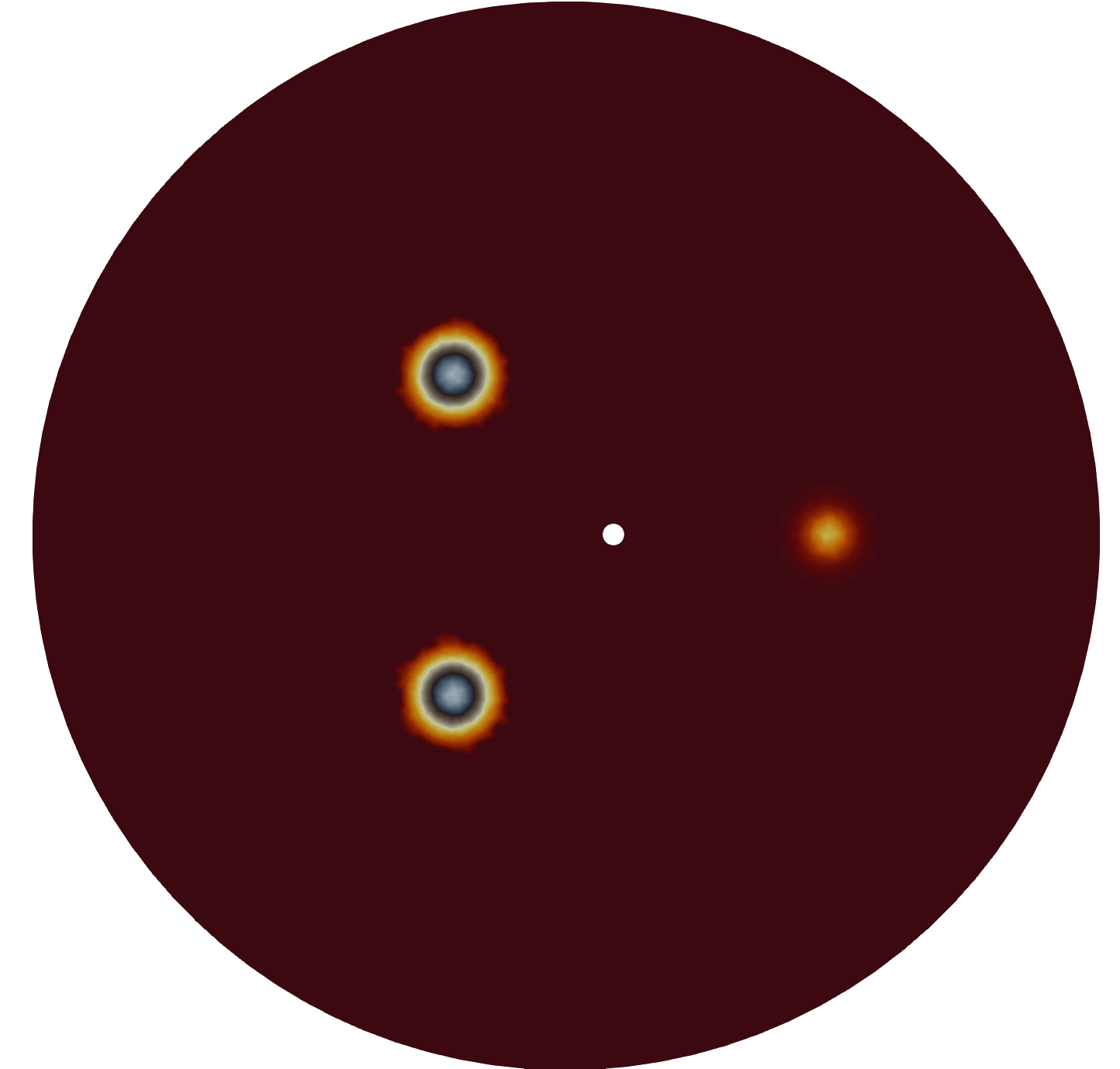
(a) $t=0$

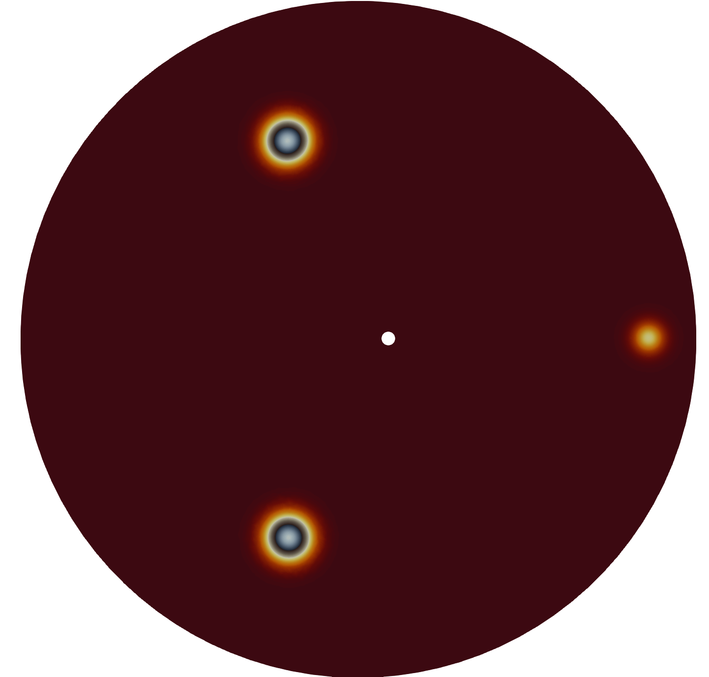
(b) $t=1998$

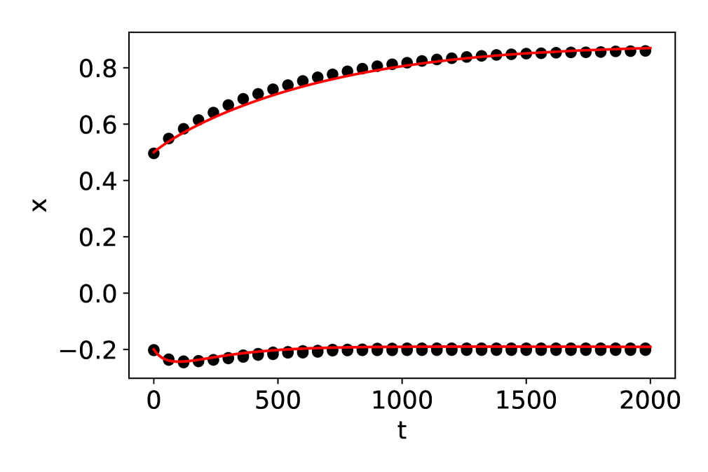
(c) $x$-coordinate of spots

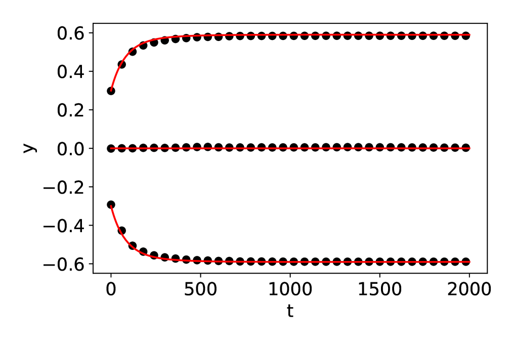
(d) $y$-coordinate of spots

Figure 6: For $\varepsilon=0.02,\,D=\tau=1,\,a=20$ and a hole at $\mathbf{x}_{0}=(0.1,0)$ with radius $\varepsilon$ ($C=1$), three spots are initially located at $(0.5,0)$ ($S\approx 0.4043$) and $(-0.2,\pm 0.3)$ ($S\approx 3.2549$), respectively. In (a) and (b), we show the numerical PDE solution of $v$ at $t=0$ and $t=1998$, respectively. In (c) and (d), we show the very close agreement of spot trajectories obtained by the PDE simulation (black dots) and the DAE (3.16) and (3.14) (red solid line). We note that the $x$-coordinates of two spots on the left of the hole almost coincide and their trajectories in the $x$-direction are indistinguishable.

In the unit disk, in Fig. 5 and Fig. 6 we show a very favorable comparison between the spot trajectories as computed from the DAE system (3.16) and (3.14) and from the full PDE system (3.1) for the case of two or three spots, respectively. The hole location and radius, and the other parameter values, are given in the figure captions. From Fig. 5 and Fig. 6, we observe that there is a repulsive interaction between the spots and the small hole. By increasing the feed-rate parameter $a$, in Fig. 7 we show that a one-spot solution will exhibit spot self-replication when the spot source strength exceeds the peanut-splitting threshold $\Sigma_{2}\approx 4.302$. However, in contrast to the case of a hole-free unit disk where the critical feed-rate parameter for the onset of a peanut-instability of a spot is $a_{c}=2\Sigma_{2}\approx 8.6$, and is independent of the spot location, we observe from Fig. 7 that a much larger feed rate is needed to trigger a peanut-splitting instability when the domain contains a hole. Moreover, the required threshold of the feed rate depends on the relative locations of the spot and the center of the hole.

3.2 Linear stability analysis

In this subsection we analyze the linear stability on an ${\mathcal{O}}(1)$ time-scale of the quasi-equilibria, denoted by $v_{e}$ and $u_{e}$, as constructed in §3.1. We substitute $v=v_{e}+e^{\lambda t}\phi$ and $u=u_{e}+e^{\lambda t}\eta$ into (3.1a) and (3.1b), and linearize to obtain

$$\begin{split}\varepsilon^{2}\Delta\phi-\phi+2u_{e}v_{e}\phi+v_{e}^{2}\eta=\lambda\phi\,,&\qquad D\Delta\eta+a-\varepsilon^{-2}\left(2u_{e}v_{e}\phi+v_{e}^{2}\eta\right)=\tau\lambda\eta\,,\quad\mbox{in}\quad\bar{\Omega}\,,\\ \partial_{n}\phi=\partial_{n}\eta=0\quad\mbox{on}\quad\partial\Omega\,;&\qquad\phi=\eta=0\quad\mbox{on}\quad\partial\Omega_{\varepsilon}\,.\end{split}$$ (3.17)

Following the analysis in §2.2, we obtain the local eigenvalue problem (2.20). The analysis of instabilities associated with non-radially symmetric perturbations near a spot is the same as given in §2.2 and the criterion is based on the source strengths. We conclude that the $j^{\mbox{th}}$ spot is linearly unstable to the peanut-splitting mode when $S_{j}>\Sigma_{2}\approx 4.302$, where $S_{j}$ is obtained from the nonlinear algebraic system (3.14) that depends on the location of the hole.

We focus on deriving a GCEP associated with radially symmetric perturbation near a spot, in which $m=0$ in the local problem (2.20). Using the distributional limit (2.24), we obtain for $\lambda\neq 0$ that the outer problem for $\eta$ away from the spots is

$$\Delta\eta-\frac{\tau\lambda}{D}\eta-\frac{2\pi}{D}\sum\limits^{N}_{i=1}c_{j}\delta(\mathbf{x}-\mathbf{x}_{i})=0\quad\mbox{in}\quad\bar{\Omega}\,,\qquad\partial_{n}\eta=0\quad\mbox{on}\quad\partial\Omega\,;\qquad\eta=0\quad\mbox{on}\quad\partial\Omega_{\varepsilon}\,.$$ (3.18)

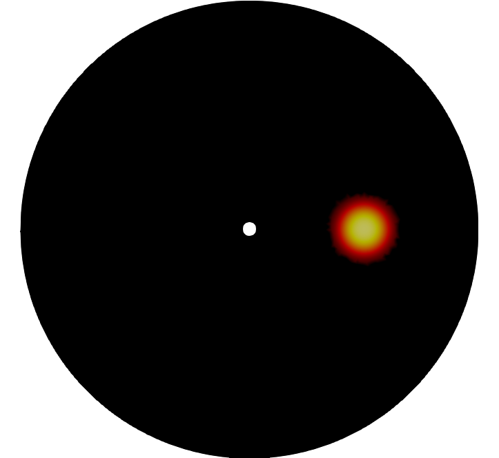
(a) $t=0$

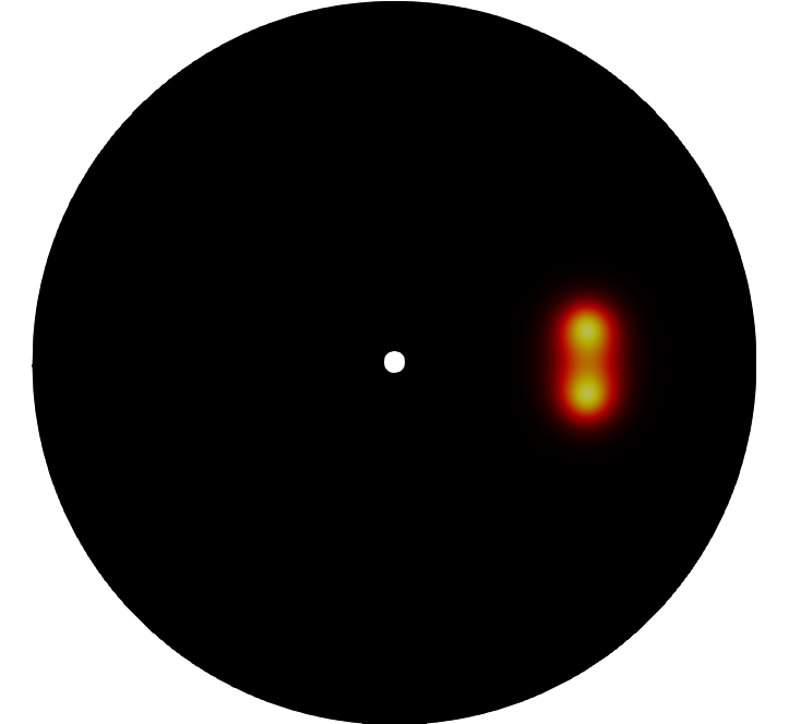
(b) $t=28$

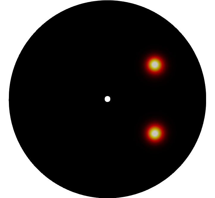
(c) $t=80$

Figure 7: For $\varepsilon=0.03\,,\tau=D=1\,,a=18$ and a hole at the center with radius $\varepsilon\,(C=1)$, a spot located at $\mathbf{x}=(0.5,0)$ initially has source strength $S\approx 4.42779$, which is greater than the peanut-splitting threshsold $\Sigma_{2}\approx 4.302$ in §2.2. We confirm the predicted spot-splitting event with this PDE simulation.

Similar to the derivation of outer problem (3.6), we approximate the zero Dirichlet boundary condition for $\eta$ on the hole boundary by a Dirac Delta forcing of undetermined strength $2\pi c_{0}D^{-1}\,\delta(\mathbf{x}-\mathbf{x}_{0})$. In this way, the modified outer problem for $\eta$ defined at ${\mathcal{O}}(1)$ distances from the spots and the hole is

$$\Delta\eta-\frac{\tau\lambda}{D}\eta-\frac{2\pi}{D}\sum\limits^{N}_{i=0}c_{i}\,\delta(\mathbf{x}-\mathbf{x}_{i})=0\quad\mbox{in}\quad\Omega\,,\qquad\partial_{n}\eta=0\quad\mbox{on}\quad\partial\Omega\,,$$ (3.19)

which is subject to the matching condition

$$\eta\sim\frac{c_{0}}{D}\left(\log|\mathbf{x}-\mathbf{x}_{0}|+\frac{1}{\nu}-\log C\right)\,,\quad\mbox{as}\quad\mathbf{x}\to\mathbf{x}_{0}\,.$$ (3.20)

The solution to (3.19) is represented in terms of the eigenvalue-dependent Green’s function $G_{\lambda}$ of (2.27) by

$$\eta=-\frac{2\pi}{D}\sum\limits_{i=0}^{N}c_{i}G_{\lambda}(\mathbf{x};\mathbf{x}_{i})\,.$$ (3.21)

We let $\mathbf{x}\to\mathbf{x}_{0}$ in (3.21) and equate the resulting ${\mathcal{O}}(1)$ limiting behavior with (3.20). This matching condition yields that

$$c_{0}+2\pi\nu\left(c_{0}R_{\lambda_{0,0}}+\sum\limits_{i=1}^{N}c_{i}\,G_{\lambda_{0,i}}\right)-\nu c_{0}\log C=0\,,$$ (3.22)

where $R_{\lambda_{0,0}}\equiv R_{\lambda}(\mathbf{x}_{0};\mathbf{x}_{0})$ and $G_{\lambda_{0,i}}\equiv G_{\lambda}(\mathbf{x}_{0};\mathbf{x}_{i})$.

Next, by expanding (3.21) as $\mathbf{x}\to\mathbf{x}_{j}$, we have for each $j=1,\ldots,N$ that

$$\eta\sim\frac{c_{j}}{D}\log|\mathbf{x}-\mathbf{x}_{j}|-\frac{2\pi}{D}\left(c_{j}R_{\lambda}(\mathbf{x}_{j};\mathbf{x}_{j})+\sum\limits_{i\neq j}^{N}c_{i}\,G_{\lambda}(\mathbf{x}_{j};\mathbf{x}_{i})+c_{0}\,G_{\lambda}(\mathbf{x}_{j};\mathbf{x}_{0})\right)\,.$$ (3.23)

Upon matching (3.23) with the far-field behavior (2.25b) of the inner problem we obtain

$$c_{j}+2\pi\nu\left(c_{j}R_{\lambda_{j,j}}+\sum\limits_{i=1,i\neq j}^{N}c_{i}\,G_{\lambda{j,i}}+c_{0}\,G_{\lambda_{j,0}}\right)+\nu c_{j}\tilde{B}(S_{j};\lambda)=0\,,$$ (3.24)

where $R_{\lambda_{j,j}}\equiv R_{\lambda}(\mathbf{x}_{j};\mathbf{x}_{j})$ and $G_{\lambda{j,i}}\equiv G_{\lambda}(\mathbf{x}_{j};\mathbf{x}_{i})$.

We write (3.22) and (3.24) in matrix form as

$$\theta_{\lambda}c_{0}+2\pi\nu\,\mathbf{g}_{\lambda}^{T}\mathbf{c}=\mathbf{0}\,,\qquad\mathbf{c}\,+\,2\pi\nu\left(\mathcal{G}_{\lambda}\mathbf{c}+c_{0}\mathbf{g}_{\lambda}\right)+\nu\tilde{\mathcal{B}}\mathbf{c}=\mathbf{0}\,,$$ (3.25a)

where the matrices $$\mathcal{G}_{\lambda} \tilde{\mathcal{B}}$$ and are defined in (2.29b). In (3.25a) we have defined

$$\mathbf{c}\equiv\left(c_{1},\ldots,c_{N}\right)^{T}\,,\quad\mathbf{g}_{\lambda}\equiv\left(G_{\lambda_{0,1}},\ldots,G_{\lambda_{0,N}}\right)^{T}\,,\quad\mathbf{e}\equiv(1,\ldots,1)^{T}\in\mathbb{R}^{N}\,,\quad\theta_{\lambda}\equiv 1+2\pi\nu R_{\lambda_{0,0}}-\nu\log C\,.$$ (3.25b)

The GCEP is obtained by eliminating $c_{0}$ in (3.25a). In this way, we conclude that a discrete eigenvalue $\lambda$ of the linearization must be such that

$$\mathcal{M}\mathbf{c}=0\,,\qquad\mbox{where}\qquad\mathcal{M}(\lambda)\equiv\theta_{\lambda}\left(\mathcal{I}+2\pi\nu\mathcal{G}_{\lambda}+\nu\tilde{\mathcal{B}}\right)-4\pi^{2}\nu^{2}\,\mathbf{g}_{\lambda}\mathbf{g}_{\lambda}^{T}\,,$$ (3.26a)

has a nontrivial solution $$\mathbf{c}\neq\mathbf{0} \mathcal{I} N\times N \lambda\neq 0$$. Here is the identity matrix. Any such satisfying

$$\det\mathcal{M}(\lambda)=0\,,$$ (3.26b)

for which $\mbox{Re}(\lambda)>0$, corresponds to an instability associated with locally radially symmetric perturbations near the spots.

As similar to the analysis in §2.2, we must consider separately the special case of a zero-eigenvalue crossing where $\lambda=0$. When $\lambda=0$, the solution to the modified outer problem (3.19) is

$$\eta=-\frac{2\pi}{D}\sum\limits_{i=0}^{N}c_{i}\,G(\mathbf{x};\mathbf{x}_{i})+\bar{\eta}\,,\qquad\mbox{where}\qquad\sum_{i=0}^{N}c_{i}=0\,,$$ (3.27)

and where $\bar{\eta}$ is an additive constant to be found. Here, $G$ is the Neumann Green’s function satisfying (2.9). By matching the local behavior of $\eta$ to the far-field behavior (3.20) near the hole as well as to the far field behavior (2.25b) near the spots, we obtain in matrix form that

$$\theta c_{0}+2\pi\nu\mathbf{g}^{T}\mathbf{c}=\nu D\bar{\eta}\,,\qquad\mathbf{c}+2\pi\nu\left(\mathcal{G}\mathbf{c}+c_{0}\mathbf{g}\right)+\nu\tilde{\mathcal{B}}_{0}\mathbf{c}=\nu D\,\bar{\eta}\,\mathbf{e}\,,$$ (3.28a)

where $$\mathcal{G}\in\mathbb{R}^{N\times N} \tilde{\mathcal{B}}_{0}=\mbox{diag}\left(\chi^{\prime}(S_{1}),\ldots,\chi^{\prime}(S_{N})\right)$$ is the Neumann Green’s matrix and , as is given in (2.36). In (3.28a) we have defined

$$\mathbf{c}\equiv\left(c_{1},\ldots,c_{N}\right)^{T}\,,\quad\mathbf{g}\equiv\left(G_{0,1},\ldots,G_{0,N}\right)^{T}\,,\quad\mathbf{e}\equiv(1,\ldots,1)^{T}\in\mathbb{R}^{N}\,,\quad\theta\equiv 1+2\pi\nu R(\mathbf{x}_{0};\mathbf{x}_{0})-\nu\log C\,,$$ (3.28b)

where $G_{0,i}\equiv G(\mathbf{x}_{0};\mathbf{x}_{i})$. Since $\sum_{i=0}^{N}c_{i}=0$, we can write $c_{0}=-\mathbf{e}^{T}\mathbf{c}$. Upon eliminating $c_{0}$ in (3.28a), we conclude that $\lambda=0$ is an eigenvalue of the linearization if and only if

$$\mathcal{M}_{0}\mathbf{c}=0\,,\qquad\mbox{where}\qquad\mathcal{M}_{0}\equiv\mathcal{I}+\theta N\mathcal{E}+2\pi\nu\,\mathcal{G}+\nu\tilde{\mathcal{B}}_{0}-2\pi\nu\left(\mathbf{g}\mathbf{e}^{T}+\mathbf{e}\mathbf{g}^{T}\right)\,,$$ (3.29)

has a nontrivial solution $\mathbf{c}\neq\mathbf{0}$. Parameter values corresponding to zero-eigenvalue crossings are where $\det\mathcal{M}_{0}=0$.

3.3 A ring pattern of $N$-spots with leakage at the center

We consider a ring pattern of $N$-spots, with spots centered at (2.39), in the perforated unit disk $\bar{\Omega}$ that has a hole of radius $C\varepsilon$ at the origin. Since the $N$ spots have a common source strength $S_{c}$, we let $\mathbf{s}=S_{c}\,\mathbf{e}$ in (3.14). Upon using ${\mathcal{G}}\mathbf{e}={p(r_{0})\mathbf{e}/N}$ from (A.3), where $r_{0}$ is the ring radius, together with

$$\theta=1+2\pi\nu R(\mathbf{0};\mathbf{0})-\nu\log C=1-\nu\left(\log C+\frac{3}{4}\right)\,,\qquad\mathbf{g}=G(\mathbf{x}_{j};\mathbf{0})\,\mathbf{e}=\frac{1}{2\pi}\left(-\log r_{0}+\frac{r_{0}^{2}}{2}-\frac{3}{4}\right)\mathbf{e}\,,$$ (3.30)

as calculated from (A.1), we obtain from (3.14) and (3.8) that $S_{c}$ satisfies the scalar nonlinear equation

$$S_{c}+\frac{\nu S_{c}}{N+1}\log\left[\frac{r_{0}^{N+1}}{NC^{N}(1-r_{0}^{2N})}\right]+\frac{\nu\chi(S_{c})}{N+1}=\frac{p_{a}}{N+1}\left[1+\nu\left(\log\left(\frac{r_{0}}{C}\right)-\frac{r_{0}^{2}}{2}\right)\right]\,,\qquad p_{a}=\frac{a}{2\sqrt{D}}\,.$$ (3.31)

Next, by using (A.2), we calculate for a ring pattern that

$$2\pi\left(p_{a}-\sum\limits_{i=1}^{N}S_{i}\right)\nabla_{\mathbf{x}}G_{j,0}=(p_{a}-NS_{c})\left(r_{0}-\frac{1}{r_{0}}\right)\mathbf{e}_{\theta_{j}}\,,$$

where $\mathbf{e}_{\theta_{j}}$ is defined in (2.39). Upon using this result, together with the expression (A.4) for $\beta_{j}$ for a ring pattern, the ODE system (3.16) for slow spot dynamics reduces to the following scalar ODE for the ring radius $r_{0}$:

$$\frac{dr_{0}}{d\sigma}=\gamma(S_{c})\left[p_{a}\left(\frac{1}{r_{0}}-r_{0}\right)-S_{c}\left(\frac{N+1}{2r_{0}}+\frac{Nr_{0}^{2N-1}}{1-r_{0}^{2N}}\right)\right]\,,$$ (3.32)

where $\sigma=\varepsilon^{2}t$. Here $S_{c}=S_{c}(r_{0})$ is determined from the nonlinear constraint (3.31). It follows that the equilibrium ring radius $r_{0}=r_{0e}$ of (3.32) with common source strength $S_{c}$ is a root of

$$S_{c}\left(\frac{N+1}{2r_{0e}}+\frac{Nr_{0e}^{2N-1}}{1-r_{0e}^{2N}}\right)=p_{a}\left(\frac{1}{r_{0e}}-r_{0e}\right)\,,$$ (3.33)

where $S_{c}=S_{c}(r_{0e})$ satisfies (3.31).

Next, the GCEP (3.26a) for a ring pattern reduces to finding values of $\lambda$ for which there are nontrivial solutions to

$$\mathcal{M}\mathbf{c}=\mathbf{0}\,,\qquad\mbox{with}\qquad\mathcal{M}\equiv\theta_{\lambda}\left(1+\nu\tilde{B}_{c}\,\mathcal{I}+2\pi\nu\,\mathcal{G}_{\lambda}\right)-4N\pi^{2}\nu^{2}\beta_{\lambda}^{2}\mathcal{E}\,,\qquad\mathcal{E}\equiv\frac{1}{N}\mathbf{e}\mathbf{e}^{T}\,,$$ (3.34)

where $\tilde{B}_{c}\equiv\tilde{B}(S_{c};\lambda)$ is calculated from (2.22) and where $\beta_{\lambda}\equiv G_{\lambda}(\mathbf{x}_{1};\mathbf{0})=\ldots=G_{\lambda}(\mathbf{x}_{N};\mathbf{0})$. Since $\mathcal{G}_{\lambda}$ is a cyclic symmetric matrix, it has the eigenspace $\mathbf{c}=\mathbf{e}$ and $\mathbf{c}=\mathbf{q}_{j}$, where $\mathbf{e}^{T}\mathbf{q}_{j}=0$ and $\mathbf{q}_{j}^{T}\mathbf{q}_{i}=0$ for $i\neq j$ and $i,j=2,\ldots,N$. In this way, from (3.34), the discrete eigenvalues $\lambda$ for the synchronous ($\mathbf{c}=\mathbf{e}$) mode and competition modes ($\mathbf{c}=\mathbf{q}_{j}$, $j=2,\ldots,N$) are the roots of

$$F_{1}\equiv\theta_{\lambda}(1+\nu\tilde{B}_{c}+2\pi\nu\,\omega_{1})-4N\pi^{2}\nu^{2}\beta_{\lambda}=0\,,$$ (3.35a)

$$F_{j}\equiv\theta_{\lambda}(1+\nu\tilde{B}_{c}+2\pi\nu\,\omega_{j})=0\,,\quad j=2\,,\ldots\,,N\,,$$ (3.35b)

where the matrix eigenvalues $\omega_{i}=\omega_{i}(\lambda)$ of $\mathcal{G}_{\lambda}$ are defined by $\mathcal{G}_{\lambda}\mathbf{e}=\omega_{1}\,\mathbf{e}$ and $\mathcal{G}_{\lambda}\mathbf{q}_{i}=\omega_{i}\,\mathbf{q}_{i}$ for $i=2,\ldots,N$.

Next, we derive the threshold condition on the parameters for which there is a zero-eigenvalue crossing in the GCEP. We use $\tilde{\mathcal{B}}_{0}=\tilde{B}(S_{c};0)\,\mathcal{I}\equiv\chi^{\prime}(S_{c})\,\mathcal{I}$, together with (3.30), to obtain that (3.29) reduces to

$$\mathcal{M}_{0}\mathbf{c}=0\,,\qquad\mbox{where}\qquad\mathcal{M}_{0}\equiv\left[1+\nu\chi^{\prime}(S_{c})\right]\,\mathcal{I}+N\left[1-\nu\left(\log\frac{C}{r_{0}^{2}}+r_{0}^{2}-\frac{3}{4}\right)\right]\mathcal{E}+2\pi\nu\,\mathcal{G}\,.$$ (3.36)

By using (A.3), we conclude from (3.36) that a zero-eigenvalue crossing for the mode $\mathbf{c}=\mathbf{e}$ occurs if and only if $S_{c}$ satisfies

$$N+1+\nu\chi^{\prime}(S_{c})+\nu\log\left(\frac{r_{0}^{N+1}}{NC^{N}(1-r_{0}^{2N})}\right)=0\,.$$ (3.37)

We now show that this zero-eigenvalue threshold condition (3.37) occurs precisely at the value of $S_{c}$ for which the root $S_{c}=S_{c}(r_{0})$ to (3.31) has a saddle-node bifurcation. To see this, we differentiate (3.31) with respects to $S_{c}$ to obtain

$$\frac{\nu}{r_{0}}\left(\frac{p_{a}(C-r_{0}^{2})}{r_{0}}-\frac{S_{c}(N+1+(N-1)r_{0}^{2N})}{r_{0}(1-r_{0}^{2N})}\right)\frac{dr_{0}}{dS_{c}}=N+1+\nu\chi^{\prime}(S_{c})+\nu\log\left(\frac{r_{0}^{N+1}}{NC^{N}(1-r_{0}^{2N})}\right)\,.$$ (3.38)

At a saddle-point point $(r_{0f},S_{cf})$ we have ${dr_{0}/dS_{c}}=0$, and so the right-hand side of (3.38) must vanish at that point, which yields (3.37). We conclude that a zero-eigenvalue crossing of the GCEP can only occur at the location of a saddle-node bifurcation point for a quasi-equilibrium ring pattern.

Next, to determine the threshold condition on the parameters for a zero-eigenvalue crossing for the competition modes, we substitute $\mathbf{c}=\mathbf{q}_{i}$ for $i=2,\ldots,N$ into (3.36), and use $\mathcal{E}\mathbf{q}_{i}=0$ to obtain

$$1+\nu\chi^{\prime}(S_{c})+2\pi\nu\sigma_{i}=0\,,\qquad i=2,\ldots,N\,.$$ (3.39)

Here $\sigma_{i}$ are eigenvalues of the Neumann Green’s matrix for which ${\mathcal{G}}\mathbf{q}_{i}=\sigma_{i}\mathbf{q}_{i}$ for $i=2,\ldots,N$. Roots of the coupled problem (3.39) and (3.30) correspond to the threshold values $(S_{c}^{(i)},r_{0}^{(i)})$, for $i=2,\ldots,N$, where a zero-eigenvalue crossing of the GCEP occurs.

3.3.1 A one-spot quasi-equilibrium

We first consider a one-spot quasi-equilibrium solution in the perforated unit disk $\bar{\Omega}$. In this subsection, we fix $\varepsilon=0.02$ and $D=\tau=1$. By taking the ring radius $r_{0}$ as a bifurcation parameter, in Fig. 8(a) we show that (3.31) has a fold bifurcation structure for the source strength of the spot. From this figure, we observe that a one-spot quasi-equilibrium solution does not exist when the spot is too close to the center of the hole located at the origin. In contrast, when there is no hole, a one-spot quasi-equilibrium solution exists for all $r_{0}\geq 0$ in the unit disk. We have numerically verified that along the lower branch in Fig. 8(a) the GCEP (3.34) has an unstable eigenvalue, while along the upper branch it has no unstable eigenvalues. To verify these linear stability predictions of the GCEP, for a one-spot quasi-equilibrium solution with $r_{0}=0.4$ we performed full PDE simulations on (3.1) with two source strengths, as indicated in the bifurcation diagram in Fig. 8(a). The short-time evolution of the spot amplitude presented in Fig. 8(b) shows that the one-spot solution on the lower branch is quickly annihilated, while the amplitude of the spot on the upper branch is stabilized at a nearby value. These full PDE results are in agreement with the linear stability predictions based on the GCEP.

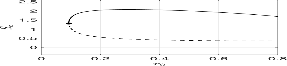
(a) Bifurcation diagram

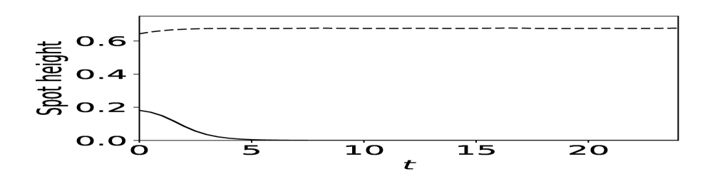
(b) Spot height

Figure 8: We fix $C=1$, $D=\tau=1$, $\varepsilon=0.02$, and $a=10$. Left panel: $S_{c}$ versus $r_{0}$ for a one-spot quasi-equilibrium solution, as computed from (3.31). The saddle-node bifurcation is at $(r_{0f},S_{cf})\approx(0.0930,1.3114)$. As indicated by (a), a one-spot pattern with $r_{0}=0.4$ has two possible source strengths, which are $S\approx 0.4094$ (lower branch) and $S\approx 2.0576$ (upper branch). Right panel: short-time evolution of the spot amplitude, defined as the maximum of $v$, with these two initial source strengths, as computed from the full PDE (3.1). The bottom (solid) curve shows that the spot on the lower branch is rapidly annihilated.

In Fig. 9(a) and Fig. 9(b), we show how the $S_{c}$ versus $r_{0}$ bifurcation diagram, computed from (3.31), changes with respect to the feed-rate parameter $a$ and the parameter $C>0$ that controls the radius $\varepsilon C$ of the hole. We observe that as either $a$ increases or $C$ decreases (smaller hole radius), a one-spot quasi-equilibrium solution can exist closer to the hole.

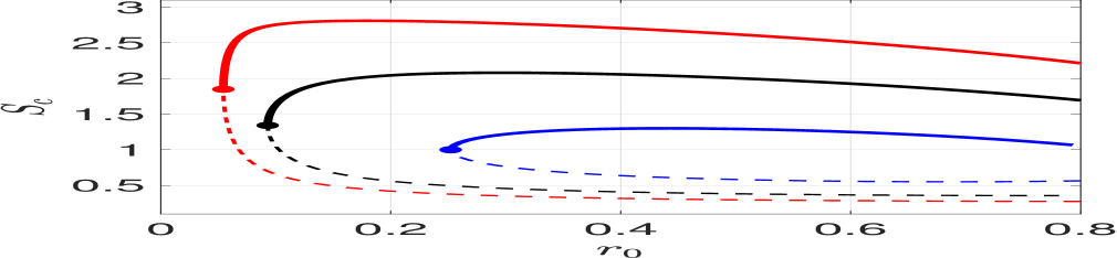
(a) Outside to inside : $a=12,\,10,\,8$.

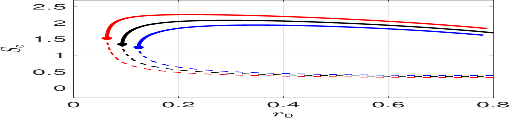
(b) Outside to inside : $C=0.8,\,1,\,1.2$.

Figure 9: In both panels, the middle curve is the same as in Fig. 8(a), which corresponds to $\varepsilon=0.02,\,C=1$ and $a=10$. All lower branches have an unstable eigenvalue for the GCEP (3.34). Left panel: We fix $C=1$. The saddle-node bifurcation for $a=8$ and $a=12$ occurs at $r_{0f}\approx 0.2521$ and $r_{0f}\approx 0.0544$, respectively. Right panel: We fix $a=10$. The saddle-node bifurcation for $C=0.8$ and $C=1.2$ occurs at $r_{0f}\approx 0.0636$ and $r_{0f}\approx 0.1243$, respectively. As either the hole radius decreases or the feed rate increases, a one-spot quasi-equilibrium solution can exist closer to the hole.

Next, we use numerical continuation on (3.31) and the saddle-node condition (3.37) to determine how the saddle-node point $r_{0f}$ for the ring radius depends on the feed-rate parameter $a$ when $C=1$. A similar numerical continuation of (3.31) and the steady-state ring radius condition (3.33), also reveals a saddle-node bifurcation structure of $r_{0e}$. These results, presented in Fig. 10(a), show that a one-spot quasi-equilibrium solution exists only when $a$ is greater than the saddle-node value $a_{f}\approx 7.4045$. For each $a>a_{f}$, there are two fold-point values of $r_{0f}$ for quasi-equilibria: one near the boundary of the unit disk (not shown in Fig. 8(a)) while the other is closer to the hole. For each $a>7.513$, there are two steady-state equilibrium ring radii, with only one of these being linearly stable for the GCEP (3.34). In Fig. 10(b), where we fixed $a=10$, we show a similar saddle-node bifurcation structure for $r_{0f}$ and $r_{0e}$ versus the parameter $C$, which controls the radius of the hole. We observe that there is no quasi-equilibrium one-spot solution if the hole radius exceeds a certain threshold.

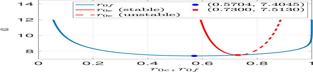
(a) Fix $C=1$

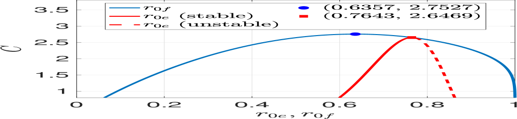
(b) Fix $a=10$

Figure 10: The saddle-node structures of $r_{0f}$ (bigger U-shape) and the equilibrium ring radius $r_{0e}$ (smaller U-shape) with respect to the feed rate $a$ (left panel) and the hole radius parameter $C$ (right panel) for a one-spot solution. Along the dashed portion of the $r_{0e}$ branch, the GCEP (3.34) has an unstable eigenvalue. For each feed-rate $a$ exceeding a threshold, there is only one stable equilibrium location for the one-spot solution.

In Fig. 11(a), we show full PDE results computed from (3.1) for a one-spot quasi-equilibrium solution, initially located at $r_{0}=0.57$, in which the feed-rate parameter is slowly decreased in time according to $a=\max(7.6-0.01\,t,\,7.4)$. From this figure, we observe that the spot amplitude collapses to zero, leading to spot annihilation, at a time $t\approx 20$. This rapid decay of the spot amplitude is due to the non-existence of one-spot quasi-equilibria for $r_{0}=0.57$ when $a$ decreases below the saddle-node value $a_{f}$. Alternatively, in Fig. 11(a), the full PDE simulation results shows that the one-spot quasi-equilibrium persists when the feed rate is fixed at $a=7.6>a_{f}$. To motivate a further, but more delicate, PDE simulation result, we observe from Fig. 10(a) that the saddle-node value for $r_{0e}$ occurs at $a_{e}\approx 7.5130$, which is greater than $a_{f}\approx 7.4045$. For any feed rate $a$ between $a_{f}$ and $a_{e}$, a quasi-equilibrium one-spot solution exists for some range of $r_{0}$, but there is no steady-state equilibrium value $r_{0e}$. In Fig. 11(b) we show results from a full PDE simulation of (3.1) for a one-spot quasi-equilibrium initially located at $r_{0}=0.57$ and with feed-rate $a=7.48$, which satisfies $a_{f}<a<a_{e}$. We observe that the one-spot quasi-equilibrium survives only until $t\approx 540$, when the slowly drifting spot is repelled sufficiently from the hole that it crosses the quasi-equilibrium existence threshold. In contrast, the corresponding PDE simulation with $a=7.6>a_{e}$ shows that the one-spot quasi-equilibrium solution persists, and slowly drifts away from the hole towards its stable equilibrium location at around $t\approx 2000$ (not shown).

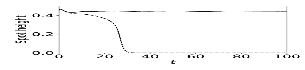
(a) $a=7.6$ v.s. $a=\max(7.6-0.01\,t,\,7.4)$

(b) $a=7.6$ v.s. $a=7.48$

Figure 11: We fix $C=1$. Left panel: Short-time evolution of the amplitude of a one-spot quasi-equilibrium solution for a constant feed rate $a=7.6$ (solid line) and for a slowly decreasing feed rate $a=\max(7.6-0.01\,t,\,7.4)$ (dashed line). Right panel: Longer time evolution of the spot amplitude for $a\equiv 7.6$ (solid line) and $a=7.48$ (dashed line). When $a=7.6$, the one-spot solution has become close to its equilibrium value when $t\approx 2000$ (not shown). For both panels the initial spot location was at $r_{0}=0.57$, and the numerical results were computed from the full PDE (3.1).

3.3.2 Hopf bifurcation of a one-spot quasi-equilibrium solution

Next, we demonstrate the occurrence of a Hopf bifurcation in the spot amplitude for a one-spot quasi-equilibrium solution in the perforated unit disk. By fixing $\varepsilon=0.02\,,a=10$, and $C=D=1$, in Fig.  12 we plot the Hopf bifurcation threshold value $\tau=\tau_{H}$ on the range $r_{0}\in[0.3,0.8]$, as obtained by numerically solving for the pair $(\tau_{H},\lambda_{I})$ from

$$\mathrm{Re}\left[F_{1}(\tau_{H},i\lambda_{I})\right]=0\,,\qquad\mathrm{Im}\left[F_{1}(\tau_{H},i\lambda_{I})\right]=0\,,$$ (3.40)

where $F_{1}$ is defined in (3.35a). In particular, when $r_{0}=0.6$, we compute that $\tau_{H}\approx 162.6$. To confirm this threshold value, in Fig. 13 we plot the spot amplitude for a one-spot quasi-equilibrium solution with $r_{0}=0.6$ for $\tau=162<\tau_{H}$, $\tau=168>\tau_{H}$, and for $\tau=170$, as computed from a full PDE simulation of (3.1). For $\tau=168$ we observe a small-scale periodic oscillation of the spot amplitude, suggesting that the Hopf bifurcation is supercritical. However, for the larger value $\tau=170$, we observe that the temporal oscillation in the spot amplitude can grow and lead to spot annihilation.

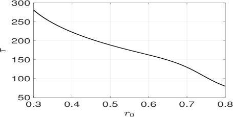
Figure 12: Hopf bifurcation threshold $\tau_{H}$ versus $r_{0}$ for a one-spot quasi-equilibrium solution, as computed from (3.40), for $a=10$, $D=C=1$, and $\varepsilon=0.02$.

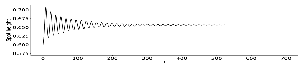
(a) $\tau=162$

(b) $\tau=168$

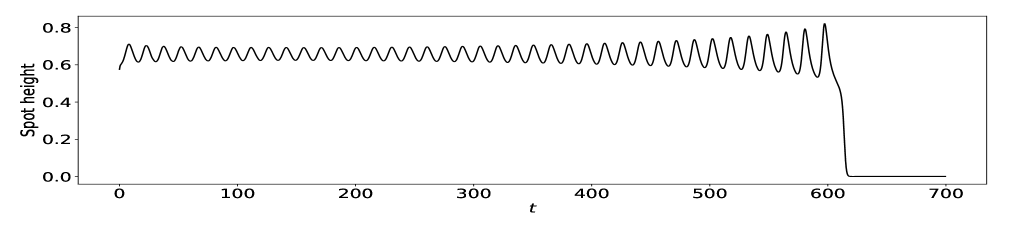
(c) $\tau=170$

Figure 13: For $\varepsilon=0.02\,,a=10\,,C=D=1$, we choose three values of $\tau$ near the Hopf bifurcation threshold $\tau_{H}\approx 162.6$ for a one-spot quasi-equilibrium solution centered at $r_{0}=0.6$. (a) $\tau=162<\tau_{H}$: the spot amplitude has decaying oscillations. (b) $\tau=168>\tau_{H}$: small amplitude oscillations indicating a supercritical Hopf bifurcation. (c) $\tau=170$: spot amplitude oscillations grow and trigger an oscillatory collapse of the spot.

3.3.3 Competition instability of a two-spot pattern

Here we consider a two-spot quasi-equilibrium pattern in the perforated unit disk, with parameters $\varepsilon=0.02,\,C=D=\tau=1$, and $a=10$. In Fig. 14, we plot the bifurcation diagram of $S_{c}$ versus $r_{0}$ for $N=2$ spots, as computed from (3.31), showing a saddle-node bifurcation behavior. We calculate that the saddle-node point occurs at $r_{0}=r_{0}^{(1)}\approx 0.1665$ and that the zero-eigenvalue crossing for the competition mode, as computed from (3.39), occurs at $r_{0}=r_{0}^{(2)}\approx 0.2573$. This naturally divides the bifurcation diagram into three segments with different stability properties: the lower branch, the upper branch on $r_{0}^{(1)}<r_{0}<r_{0}^{(2)}$, and the upper branch on $r_{0}>r_{0}^{(2)}$. On the lower branch, we compute that there is a root to $F_{1}=0$ to (3.35a) with $\mbox{Re}(\lambda)>0$, and so the GCEP (3.34) has an unstable eigenvalue. This indicates that, on the lower branch, the two-spot pattern is unstable to synchronous locally radially-symmetric perturbations near the spots. Along the upper branch with $r_{0}<r_{0}^{(2)}$ there is a root to $F_{2}=0$ in (3.35b) with $\mbox{Re}(\lambda)>0$, and so this segment of the bifurcation diagram is unstable to asynchronous locally radially-symmetric perturbations. Finally, on the upper branch with $r_{0}>r_{0}^{(2)}$, there is no root to (3.35b) in $\mbox{Re}(\lambda)>0$, and so this segment is linearly stable. These linear stability predictions are validated in Fig. 15 from full PDE simulations of (3.1) with initial conditions chosen in these three segments of the bifurcation diagram in Fig. 14.

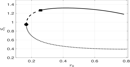
Figure 14: The saddle-node bifurcation point and the competition threshold for a two-spot ring solution are shown as black circle and square markers, respectively. The dashed (solid) segment of upper branch corresponds where $r_{0}<r_{0}^{(2)}$ ($r_{0}>r_{0}^{(2)}$). Here $r_{0}^{(2)}$ is where there is a zero-eigenvalue crossing of the GCEP (3.36) for the competition mode. The parameters are $C=D=\tau=1$, $a=10$, and $\varepsilon=0.02$.

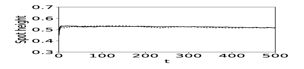
(a) Two spots survive.

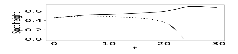
(b) One spot survives.

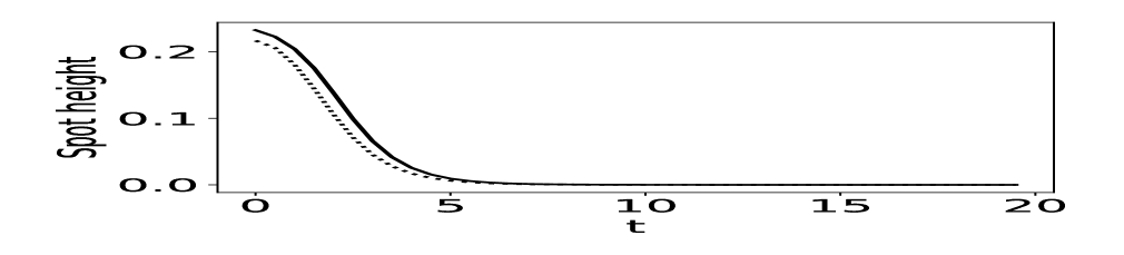
(c) Both spots die.

Figure 15: The evolution of the spot amplitudes for a two-spot quasi-equilibrium solution, as computed from the full PDE (3.1). In (a) and (b), the two spots have initial condition on the upper branch of Fig. 14. Their initial locations are at $(\pm r_{0},0)$, where $r_{0}=0.28>r_{0}^{(2)}$ and $r_{0}=0.2<r_{0}^{(2)}$ in (a) and (b), respectively. In (c), the two-spots have initial condition on the lower branch, with $r_{0}=0.29$. The parameters are $C=D=\tau=1$, $a=10$, and $\varepsilon=0.02$. The PDE results are in agreement with linear stability predictions.

4 Pinning effects from a spatially localized feed-rate

In this section, we analyze slow spot dynamics for the case where the localized heterogeneity consists of a localized source of feed from the substrate of the form

$$a(\mathbf{x})=a_{0}+\varepsilon^{-2}a_{1}\Phi\big{(}|\mathbf{x}-\boldsymbol{\xi}|/\varepsilon\big{)}\,,\qquad\Phi(r)\equiv\exp(-r^{2}/2)/(2\pi)\,,$$ (4.1)

where $a_{0}>0$ and $a_{1}>0$ are constants. Here $\boldsymbol{\xi}\in\Omega$ is the location of the concentration of the feed.

4.1 Quasi-equilibria and slow spot dynamics

We first modify our asymptotic construction of $N$-spot quasi-equilibria given in §2.1 to include the heterogeneous feed rate of (4.1). The asymptotic analysis for the inner region near a spot is exactly the same as in §2.1. Following the derivation in §2.1, the outer problem for the inhibitor field, defined away from the spots, is

$$\Delta u+\frac{a(\mathbf{x})}{D}-\frac{2\pi}{\sqrt{D}}\sum\limits_{i=1}^{N}S_{i}\,\delta(\mathbf{x}-\mathbf{x}_{i})=0\quad\mbox{in}\quad\Omega\,,\qquad\partial_{n}u=0\quad\mbox{on}\quad\partial\Omega\,,$$ (4.2)

where $S_{1},\ldots,S_{N}$ are the source strengths of the $N$ spots. By applying the divergence theorem to (4.2) we get

$$\sum\limits_{i=1}^{N}S_{i}=\frac{\int_{\Omega}a\,d\mathbf{x}}{2\pi\sqrt{D}}\equiv p_{a}\,.$$ (4.3)

We decompose the solution to (4.2) as

$$u(\mathbf{x})=\frac{u_{2}(\mathbf{x})}{D}-\frac{2\pi}{\sqrt{D}}\sum\limits_{i=1}^{N}S_{i}G(\mathbf{x};\mathbf{x}_{i})+\bar{u}\,,$$ (4.4)

where $\bar{u}$ is a constant and $G$ is the Neumann Green’s function of (2.9). Here $u_{2}(\mathbf{x})$ is the unique solution to

$$\Delta u_{2}=-a(\mathbf{x})+\frac{\int_{\Omega}a(\mathbf{x})d\mathbf{x}}{|\Omega|}\quad\mbox{in}\quad\Omega\,,\quad\partial_{n}u_{2}=0\quad\mbox{on}\quad\partial\Omega\,;\qquad\int_{\Omega}u_{2}\,dx=0\,,$$ (4.5)

which is given in terms of $G$ by

$$u_{2}(\mathbf{x})=\int_{\Omega}a(\mathbf{z})\,G(\mathbf{z};\mathbf{x})\,d\mathbf{z}\,.$$ (4.6)

As in §2.1 we can perform an asymptotic matching as $\mathbf{x}\to\mathbf{x}_{j}$ for $j=1,\ldots,N$ between the outer solution and inner solutions to derive a nonlinear algebraic system for $\bar{u}$ and the source strengths. Letting $\mathbf{x}\to\mathbf{x}_{j}$ in (4.4), we obtain that

$$\begin{split}u&\sim\frac{u_{2}(\mathbf{x}_{j})}{D}+\frac{S_{j}}{\sqrt{D}}\log|\mathbf{x}-\mathbf{x}_{j}|-\frac{2\pi}{\sqrt{D}}\left(S_{j}R_{j,j}+\sum\limits_{i\neq j}^{N}S_{i}G_{j,i}\right)+\bar{u}\\ &\quad+\left(\frac{1}{D}\,\nabla_{\mathbf{x}}u_{2}(\mathbf{x}_{j})-\frac{2\pi}{\sqrt{D}}\left(S_{j}\nabla_{\mathbf{x}}R_{j,j}+\sum\limits_{i\neq j}^{N}S_{i}\nabla_{\mathbf{x}}G_{j,i}\right)\right)\cdot(\mathbf{x}-\mathbf{x}_{j})+{\mathcal{O}}(|\mathbf{x}-\mathbf{x}_{j}|^{2})\,,\qquad j=1,\ldots,N\,,\end{split}$$ (4.7)

where $R_{j,j}\equiv R(\mathbf{x}_{j};\mathbf{x}_{j})$ and $G_{j,i}\equiv G(\mathbf{x}_{j};\mathbf{x}_{i})$.

Upon matching (4.7) with (2.10) for the $\mathcal{O}(1)$ terms, we write the resulting equations in matrix form as

$$\mathbf{s}+2\pi\nu\,\mathcal{G}\mathbf{s}+\nu\bm{\chi}=\nu\left(\frac{1}{\sqrt{D}}\,\mathbf{u_{2}}+\bar{u}\sqrt{D}\,\mathbf{e}\right)\,,\qquad\mathbf{e}^{T}\mathbf{s}=p_{a}\,,$$ (4.8a)

where $$\mathcal{G}$$ is the Neumann Green’s matrix, and where we have defined

$$\mathbf{s}\equiv(S_{1},\ldots,S_{N})^{T}\,,\quad\bm{\chi}\equiv(\chi(S_{1}),\ldots,\chi(S_{N}))^{T}\,,\quad\mathbf{e}\equiv(1,\ldots,1)^{T}\in\mathbb{R}^{N}\,,\quad\mathbf{u}_{2}\equiv(u_{2}(\mathbf{x}_{1}),\ldots,u_{2}(\mathbf{x}_{N}))^{T}\,.$$ (4.8b)

Upon left-multiplying (4.8a) by $\mathbf{e}^{T}$, we can isolate $\bar{u}$ as

$$\bar{u}=\frac{p_{a}+2\pi\nu\,\mathbf{e}^{T}\mathcal{G}\mathbf{s}+\nu\,\mathbf{e}^{T}\bm{\chi}}{\nu N\sqrt{D}}-\frac{\mathbf{e}^{T}\mathbf{u}_{2}}{ND}\,.$$ (4.9)

By using (4.9) to eliminate $\bar{u}$ in (4.8a), we obtain a nonlinear algebraic system for the vector of source strengths $\mathbf{s}$,

$$\mathbf{s}+2\pi\nu(I-\mathcal{E})\,\mathcal{G}\mathbf{s}+\nu(I-\mathcal{E})\bm{\chi}=\frac{\nu}{\sqrt{D}}\,(I-\mathcal{E})\mathbf{u}_{2}+\frac{p_{a}}{N}\mathbf{e}\,,\qquad\mbox{where}\qquad\mathcal{E}=\frac{1}{N}\mathbf{e}\mathbf{e}^{T}\,,$$ (4.10)

and $p_{a}$ is defined in (4.3).

To derive the DAE system for slow spot dynamics we must match (2.10) with (4.7) for the $\mathcal{O}(\varepsilon)$ gradient terms. This matching yields the far-field behavior for the inner correction term $U_{j1}$, as defined in (2.1), given by

$$U_{j1}\sim\left(\frac{1}{\sqrt{D}}\,\nabla_{\mathbf{x}}u_{2}(\mathbf{x}_{j})-\boldsymbol{\beta}_{j}\right)\cdot\,\mathbf{y}\,\quad\mbox{as}\quad|\mathbf{y}|\to\infty\,,$$ (4.11)

where $\mathbf{y}=\varepsilon^{-1}(\mathbf{x}-\mathbf{x}_{j})$ and $\boldsymbol{\beta}_{j}$ is defined in (2.12). Following the derivation in §2.1, we conclude that the DAE system for slow spot dynamics is given by

$$\frac{d\mathbf{x}_{j}}{d\sigma}=\gamma(S_{j})\left(\frac{1}{\sqrt{D}}\,\nabla_{\mathbf{x}}u_{2}(\mathbf{x}_{j})-\boldsymbol{\beta}_{j}\right)\,,\qquad j=1,\ldots,N\,,$$ (4.12)

where $\sigma=\varepsilon^{2}t$ and $\mathbf{s}\equiv(S_{1},\ldots,S_{N})^{T}$ satisfies the nonlinear algebraic system (4.10). Here $\gamma(S_{j})$ is defined in (2.18).

As $\varepsilon\to 0$, we can approximate, in the sense of distributions, the heterogeneous feed rate in (4.1) as

$$a(\mathbf{x})\to a_{0}+a_{1}\,\delta(\mathbf{x}-\boldsymbol{\xi})\,.$$ (4.13)

In this way, $u_{2}$ in (4.6) can be calculated explicitly, by using Green’s reciprocity and $\int_{\Omega}G(\mathbf{z};\mathbf{x})\,d\mathbf{x}=0$, as

$$u_{2}(\mathbf{x})=\int_{\Omega}a(\mathbf{z})G(\mathbf{z};\mathbf{x})d\mathbf{x}=a_{1}G(\mathbf{x};\bm{\xi})\,.$$ (4.14)

4.1.1 One-spot dynamics in the unit disk

For a one-spot solution, we use (4.13) in (4.3) to calculate $S_{1}$. Then, by using (4.14) in (4.12), together with the explicit expressions (A.2) for the gradients of the Neumann Green’s function for the unit disk, we obtain from (4.12) that the slow dynamics of a one-spot quasi-equilibrium solution is

$$\frac{d\mathbf{x}_{1}}{d\sigma}=-\frac{a_{0}\gamma(S_{1})}{2\pi\sqrt{D}}\,\mathcal{H}(\mathbf{x}_{1})\,,\qquad\mbox{with}\qquad S_{1}=\frac{a_{0}\pi+a_{1}}{2\pi\sqrt{D}}\,,$$ (4.15a)

where $$\sigma=\varepsilon^{2}t \mathcal{H}$$ and is defined by

$$\mathcal{H}(\mathbf{x}_{1})\equiv\frac{a_{1}}{a_{0}}\left[\frac{\mathbf{x}_{1}-\bm{\xi}}{|\mathbf{x}_{1}-\bm{\xi}|^{2}}+\frac{\mathbf{x}_{1}|\bm{\xi}|^{2}-\bm{\xi}}{|\mathbf{x}_{1}|^{2}|\bm{\xi}|^{2}-2\mathbf{x}_{1}\cdot\bm{\xi}+1}\right]+\frac{\mathbf{x}_{1}}{1-|\mathbf{x}_{1}|^{2}}\left[\frac{a_{1}}{a_{0}}+\pi(2-|\mathbf{x}_{1}|^{2})\right]\,.$$ (4.15b)

Without loss of generality we let $\boldsymbol{\xi}=(\xi,0)$ with $0<\xi<1$. By symmetry, any equilibrium to (4.15) lies on the line that connects the origin and $\bm{\xi}$. As such, we let $\mathbf{x}_{1}=(r_{0},0)$ and obtain from (4.15) that $r_{0}=r_{0}(\sigma)$ satisfies the scalar ODE

$$\frac{dr_{0}}{d\sigma}=-\frac{a_{0}\gamma(S_{1})}{2\pi\sqrt{D}}\,\mathcal{K}(r_{0})\,,\qquad\mbox{where}\qquad\mathcal{K}(r_{0})\equiv\frac{a_{1}}{a_{0}}\left(\frac{1}{r_{0}-\xi}+\frac{r_{0}-\xi}{(1-r_{0}^{2})(1-\xi r_{0})}\right)+\frac{\pi r_{0}(2-r_{0}^{2})}{1-r_{0}^{2}}\,.$$ (4.16)

Since $\gamma(S_{1})>0$ and $\mathcal{K}(r_{0})>0$ on $\xi<r_{0}<1$, it follows that ${dr_{0}/d\sigma}<0$ on the range $\xi<r_{0}<1$.

As such, any equilibrium $r_{0e}$ for (4.16), satisfying $\mathcal{K}(r_{0e})=0$, must be on the range $0<r_{0}<\xi$. The effect of the relative magnitude of the localized feed to the background feed appears in (4.16) in the form of their ratio $a_{1}/a_{0}$. Taking this ratio as a bifurcation parameter, in Fig. 16(a) we plot the bifurcation diagram of the roots to $\mathcal{K}(r_{0})=0$ for $\xi=0.7$. We observe that there are two equilibria $r_{0e}^{(1)}<r_{0e}^{(2)}$ provided that $a_{1}/a_{0}<0.7208$, and none if ${a_{1}/a_{0}}>0.7208$. Since $\mathcal{K}^{\prime}(r_{0e}^{(1)})>0$, we conclude that $r_{0e}^{1}$ is a stable equilibrium point of (4.16), while $r_{0e}^{2}$ is an unstable equilibrium. To further demonstrate the saddle-node bifurcation value of ${a_{1}/a_{0}}$, in Fig. 16(b) we plot $\mathcal{K}(r_{0})$ on $0<r_{0}<\xi$ for the four values ${a_{1}/a_{0}}=0.3\,,0.6\,,0.72$ and $0.8$. For ${a_{1}/a_{0}}<0.7208$, we have that ${dr_{0}/d\sigma}>0$ on the range $r_{0e}^{(2)}<r_{0}<\xi$ and ${dr_{0}/d\sigma}<0$ for $\xi<r_{0}<1$. Moreover, since ${dr_{0}/d\sigma}=\mathcal{O}\left[1/(r_{0}-\xi)\right]$ as $r_{0}\to\xi$, this implies that a spot initially located at some $r_{0}(0)$ with $r_{0}(0)>r_{0e}^{(2)}$ will get pinned at the concentration point $\xi$ of the feed rate at a finite time. Moreover, if ${a_{1}/a_{0}}>0.7208$, this finite-time pinning will occur for any initial point $r_{0}(0)$ in $0<r_{0}(0)<1$.

We summarize the fate of a one-spot quasi-equilibrium solution with slow dynamics (4.16) as follows: The spot drifts to the equilibrium $r_{0}=r_{0e}^{(1)}$ for any $r_{0}(0)<r_{0e}^{(2)}$ when ${a_{1}/a_{0}}<0.7208$. The spot gets pinned at $r_{0}=\xi$ if $r_{0}(0)>r_{0e}^{(2)}$ and ${a_{1}/a_{0}}<0.7208$. The spot gets pinned at $r_{0}=\xi$ for any $r_{0}(0)$ in $0<r_{0}(0)<1$ if ${a_{1}/a_{0}}>0.7208$. We emphasize that this saddle node threshold value for ${a_{1}/a_{0}}$ is independent of the inhibitor diffusivity $D$. Although our asymptotic analysis, leading to the ODE (4.15), is only valid when the spot is well-separated from the concentration point the feed rate, i.e. when $|\mathbf{x}-\bm{\xi}|\gg{\mathcal{O}}(\varepsilon)$, the prediction of finite-time pinning phenomena provides a motivation for the analysis in §5 of constructing a new type of spot solution where the spot is pinned at the point of concentration of the feed rate.

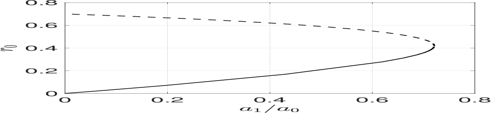
(a) Bifurcation diagram

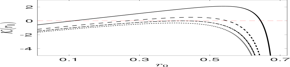
(b) $\mathcal{K}$

Figure 16: The concentration point for the feed rate is $\bm{\xi}=(0.7,0)$. Left panel: The bifurcation diagram of the equilibria $r_{0e}$ of $\mathcal{K}(r_{0})=0$, as defined in (4.16), versus ${a_{1}/a_{0}}$. A saddle-node bifurcation occurs at ${a_{1}/a_{0}}\approx 0.7208$. Right panel: From top to bottom, plots of $\mathcal{K}(r_{0})$ for $a_{1}/a_{0}=0.3\,,0.6\,,0.72$ and $0.8$, respectively.

To illustrate these results we compare predictions based on the scalar ODE (4.16) with full PDE simulations of (1.1) with the feed rate (4.1) in the unit disk with $D=\tau=1$, and $\varepsilon=0.03$. We set $\xi=0.7$ and with the choice $a_{0}=6$ and $a_{1}=4$, for which ${a_{1}/a_{0}}<0.7208$, the two equilibrium locations are $r_{0e}^{(1)}\approx 0.3178$ and $r_{0e}^{(2)}\approx 0.5090$. In Fig. 17(a), where we compare results from full PDE simulations and the ODE (4.16), we verify that a spot initially located at $r_{0}(0)=0.2<r_{0e}^{(1)}$ slowly drifts to $r_{0e}^{(1)}$. In contrast, for the same $a_{0}$ and $a_{1}$, but with initial value $r_{0}(0)=0.53>r_{0e}^{(2)}$, we observe from Fig. 17(b) that the spot approaches $\xi=0.7$. The full PDE and ODE results are found to agree well until the spot is near $\xi=0.7$. We remark that the velocity field in the ODE becomes singular as $r_{0}\to\xi$ owing to the Dirac delta function approximation of the localized feed rate. Finally, if we increase the relative strength of the concentration of the feed rate so that $a_{0}=6$ and $a_{1}=5$, for which ${a_{1}/a_{0}}>0.7208$, we confirm from Fig. 17(c) that with $r_{0}(0)=0.3$ the spot gets pinned at $\xi$ owing to the absence of any equilibrium for this ratio ${a_{1}/a_{0}}$.

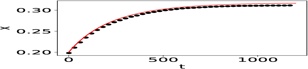
(a) Drift to $r_{0e}^{(1)}$

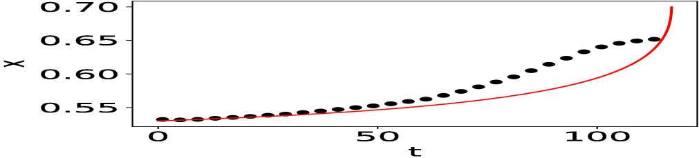
(b) Pinned at $\xi$

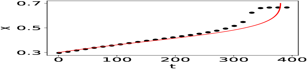
(c) Pinned at $\xi$

Figure 17: The $x$-coordinates of the spot trajectory computed from the full PDE (1.1) with (4.1) (black dots) and the scalar ODE (4.16) with $\xi=0.7$. Left panel: $a_{0}=6$, $a_{1}=4$, and $r_{0}(0)=0.2$. Middle panel: $a_{0}=6$, $a_{1}=4$, and $r_{0}(0)=0.53$. Right panel: $a_{0}=6$, $a_{1}=5$, and $r_{0}(0)=0.3$.

4.1.2 Two-spot dynamics in the unit disk

Next, we consider a ring pattern of $N$-spots in the unit disk with localized feed rate concentrated at the origin, so that $\boldsymbol{\xi}=\mathbf{0}$. By using $\nabla_{\mathbf{x}}u_{2}=a_{1}\nabla_{\mathbf{x}}G(\mathbf{x};\mathbf{0})$, together with (A.2) and (A.4) for $\nabla_{\mathbf{x}}G(\mathbf{x};\mathbf{0})$ and $\beta_{j}$, respectively, we obtain from (4.12) that the slow dynamics of the ring radius $r_{0}$ satisfies the scalar ODE

$$\frac{dr_{0}}{d\sigma}=-\frac{a_{0}\gamma(S_{c})}{2\pi r_{0}\sqrt{D}}\,\mathcal{D}(r_{0})\,,\qquad\mbox{where}\qquad\mathcal{D}(r_{0})\equiv\frac{N+1}{2N}\left[\frac{a_{1}}{a_{0}}-\pi\left(\frac{N-1}{N+1}\right)\right]+\pi r_{0}^{2}+\left(\pi+\frac{a_{1}}{a_{0}}\right)\frac{r_{0}^{2N}}{1-r_{0}^{2N}}\,.$$ (4.17)

From (4.3) and (4.13), the common spot source strength is $S_{c}={(a_{0}\pi+a_{1})/[2\pi N\sqrt{D}]}$.

The equilibrium ring radius $r_{0e}$ is a root to $\mathcal{D}(r_{0})=0$. Since $\mathcal{D}^{\prime}(r_{0})>0$ and $\mathcal{D}\to+\infty$ as $r_{0}\to 1^{-}$, the ODE (4.17) must have an equilibrium point in $0<r_{0}<1$ when

$$\mathcal{D}(0)=\frac{N+1}{2N}\left[\frac{a_{1}}{a_{0}}-\pi\left(\frac{N-1}{N+1}\right)\right]<0\,,\qquad\mbox{which implies}\qquad\frac{a_{1}}{a_{0}}<\pi\left(\frac{N-1}{N+1}\right)\,.$$ (4.18)

For $N=2$, in Fig. 18 we plot the bifurcation diagram of the equilibrium ring radius $r_{0e}$ versus the ratio ${a_{1}/a_{0}}$. On the range $0\leq{a_{1}/a_{0}}<{\pi/3}\approx 1.047$, we observe that there is a unique equilibrium radius. We note that $r_{0e}\to 0$ when ${a_{1}/a_{0}}\to\pi/3\approx 1.0472$, which is the upper bound for ${a_{1}/a_{0}}$ in (4.18) for $N=2$.

Next, we fix $a_{0}=4.3$, and $D=\tau=1$. The analysis of competition instabilities and the derivation of the GCEP for two-spot equilibria with feed concentration at the origin is exactly the same as in §2.3 provided that we use $S_{c}={(a_{0}\pi+a_{1})/[4\pi\sqrt{D}]}$ with $D=1$ for the common source spot strength. This leads to the root finding criterion (2.44) with $j=N=2$ for the GCEP (2.42) and the zero-eigenvalue crossing condition (2.46) with $j=N=2$. When $a_{1}=0$ (no feed concentration), Fig. 2(a) showed that there is a competition instability for a steady-state two-spot ring pattern if $a_{0}<4.45$. From a numerical computation of the winding number (2.32) and the zero-eigenvalue crossing condition (2.46) with $j=N=2$, we obtain that the dashed portions in the bifurcation diagram in Fig. 18 for the equilibrium ring radius correspond to where the two-spot equilibrium solution is unstable to a competition instability. As expected, since $a_{0}=4.3<4.45$, we observe that the two-spot equilibrium is unstable if $a_{1}$ is sufficiently small. Moreover, the two-spot equilibrium is unstable near ${a_{1}/a_{0}}\approx{\pi/3}$ since the spots become too closely spaced (i.e. $r_{0e}$ is too small). However, the key new qualitative feature of Fig. 18 is that there is a range of ${a_{1}/a_{0}}$ where a concentration of feed at the origin stabilizes a two-spot equilibrium solution, which without the concentration of feed would be unstable to a competition stability.

Figure 18: Bifurcation diagram of equilibrium ring radius versus the ratio ${a_{1}/a_{0}}$, as computed from setting $\mathcal{D}(r_{0})=0$ in (4.17), for a two-spot pattern in the unit disk with feed rate concentration at the origin. Fixing $a_{0}=4.3$ and $D=\tau=1$, on the range $0.1777<r_{0e}<0.4111$ (solid portion) the concentration of feed at the origin renders the two-spot equilibrium solution linearly stable to a competition instability. The dashed portions are where the solution is unstable to competition.

To illustrate this linear stability prediction for $a_{0}=4.3$ and $D=\tau=1$, we take $\varepsilon=0.02$ and perform full PDE simulations of (1.1) with (4.1) for a two-spot equilibrium ring pattern with spots located at $(\pm r_{0e},0)$. In Fig. 19(a) and Fig. 19(b) we show full PDE results for the amplitudes of the spots for the ratios ${a_{1}/a_{0}}=0.1040$ and ${a_{1}/a_{0}}=0.9932$, respectively, which lie on the unstable dashed portions in the bifurcation diagram of Fig. 18. For both values of ${a_{1}/a_{0}}$, we confirm from these figures that a competition instability occurs, which triggers the annihilation of a spot. In contrast, for ${a_{1}/a_{0}}=0.5166$, Fig. 18 predicts that the two-spot equilibrium solution, with spots centered at $(\pm 0.3345,0)$, will be linearly stable to a competition instability. This prediction is confirmed from the numerical PDE results shown in Fig. 19(c).

In Fig. 20, we show some snapshots of $v$ from the full PDE numerical solution for the parameter set in Fig. 19(b). This figure shows that after the competition instability triggers a spot-annihilation event, the surviving spot ultimately get pinned at the origin where the feed rate is concentrated. From Fig. 19(b) we observe that the spot amplitude for this pinned spot is approximately $0.8754$, which exceeds the maximum value of approximately $0.8$, as shown in Fig. 1(b), for a conventional spot solution that is not near a concentration point of the feed. This observation motivates the analysis in §5 of constructing a new type of spot solution that is pinned at the concentration point of the feed rate.

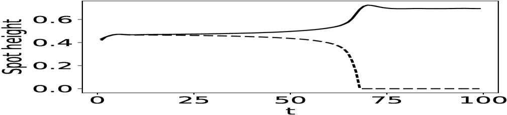
(a) $r_{0e}=0.4330\,,$ $a_{1}/a_{0}=0.1040$.

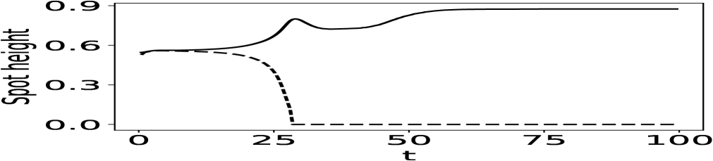
(b) $r_{0e}=0.1127\,,$ $a_{1}/a_{0}=0.9932$.

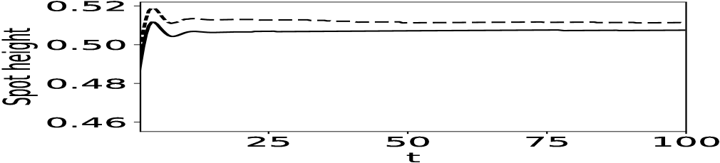
(c) $r_{0e}=0.3345\,,$ $a_{1}/a_{0}=0.5166$.

Figure 19: Full PDE simulations of (1.1) with (4.1) of the spot amplitudes for three ratios of ${a_{1}/a_{0}}$. The initial condition for the PDE is a two-spot equilibrium ring pattern with spots located at $(\pm r_{0e},0)$. Parameters are $\varepsilon=0.02$, $D=\tau=1$, and $a_{0}=4.3$. The competition instability occurring in (a) and (b), leads to spot annihilation. In (c), the two-spot equilibrium is linearly stable.

(a) $t=0$

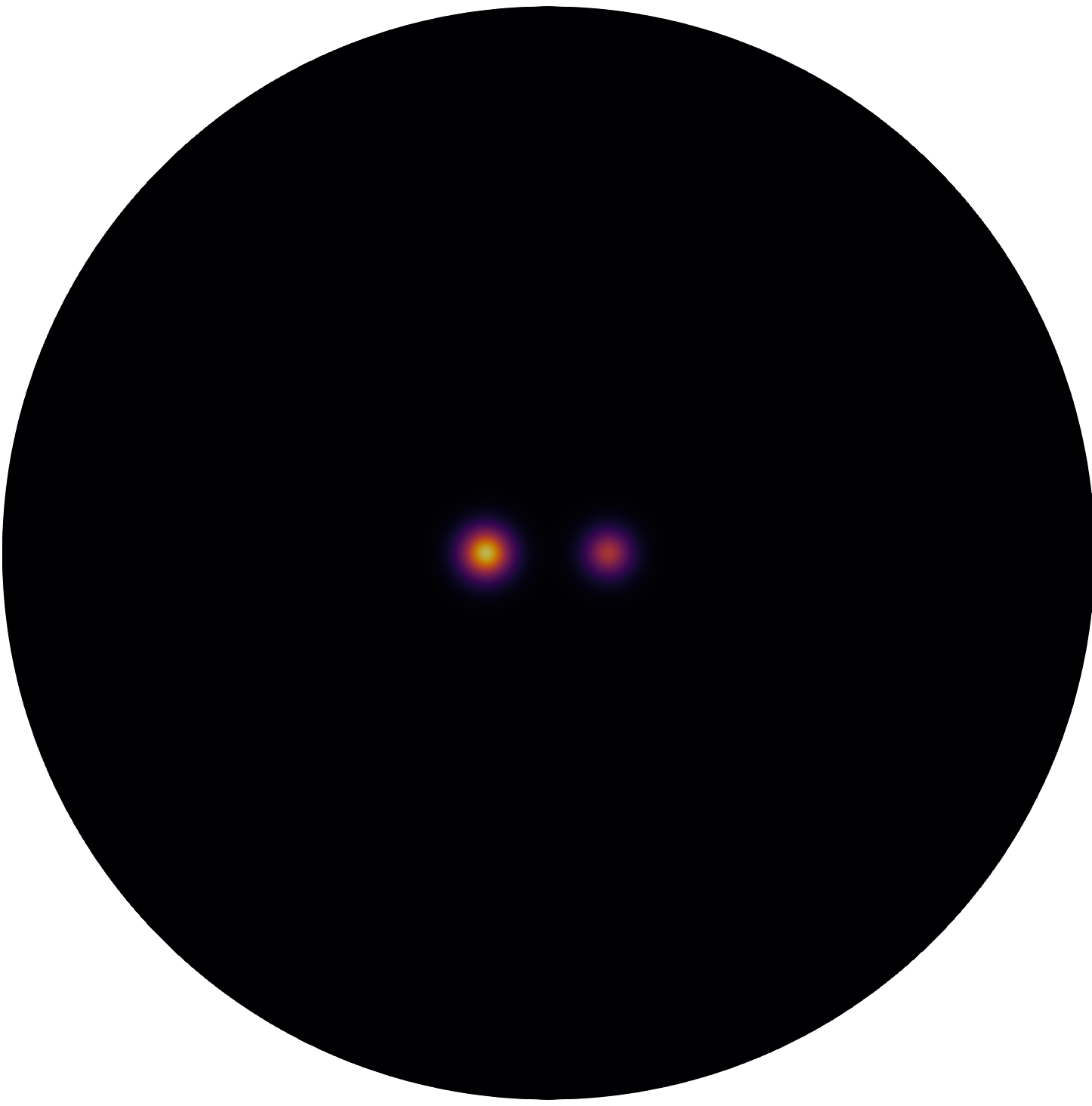
(b) $t=25$

(c) $t=29$

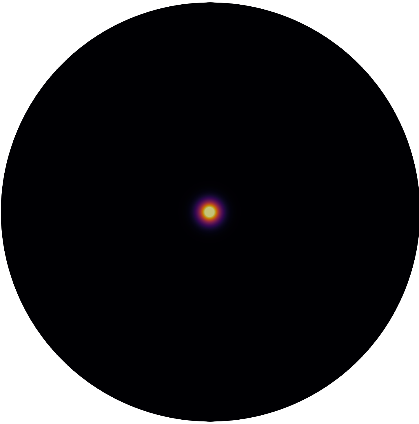
(d) $t=99$

Figure 20: Contour plots of $v$, from full PDE solutions of (1.1) with (4.1), corresponding to the parameter values shown in Fig. 19(b). A competition instability triggers spot annihilation, and the surviving spot drifts to the origin where it is pinned by the localized feed rate.

5 Spot-pinning at a localized heterogeneity: A new type of localized structure

In this section we consider the Schnakenberg model (1.1) with $D=\tau=1$ and with localized feed rate (4.1), given by

$$v_{t}=\varepsilon^{2}\Delta v-v+uv^{2}\,,\qquad u_{t}=\Delta u+a_{0}+\varepsilon^{-2}\left(a_{1}\Phi\left(\varepsilon^{-1}|\mathbf{x}-\boldsymbol{\xi}|\right)-uv^{2}\right)\quad\mbox{in}\quad\Omega\,,$$ (5.1)

with $\partial_{n}v=\partial_{n}v=0$ on $\partial\Omega$. For the choice $\Phi(r)\equiv{\exp(-r^{2}/2)/(2\pi)}$, we construct a new type of spot solution that is pinned at the site $\boldsymbol{\xi}\in\Omega$ of the localization of the feed rate. Novel dynamical behaviors associated with including this new type of spot solution in a quasi-equilibrium spot pattern are analyzed.

5.1 A pinned spot solution

We construct the asymptotic profile of a pinned spot solution and we study its linear stability properties with respect to non-radially symmetric perturbations near the spot. We then consider the effect of a time-varying localized concentration of the feed rate.

5.1.1 A quasi-equilibrium one-spot pattern

We begin by constructing an asymptotic quasi-equilibrium solution for (5.1) corresponding to a single spot pinned at $\boldsymbol{\xi}$. The quasi-equilibrium problem is

$$\varepsilon^{2}\Delta v_{e}-v_{e}+u_{e}v_{e}^{2}=0\,,\quad\Delta u_{e}+a_{0}+\varepsilon^{-2}\left[a_{1}\Phi\left(\varepsilon^{-1}|\mathbf{x}-\boldsymbol{\xi}|/\right)-u_{e}v_{e}^{2}\right]=0\,,$$ (5.2)

with $\partial_{n}v_{e}=\partial_{n}u_{e}=0$ on $\partial\Omega$ and $\Phi(r)\equiv{\exp(-r^{2}/2)/(2\pi)}$. In the inner region near the pinned spot, we look for a locally radially symmetric solution of the form $v_{e}\sim V_{0}(\rho)$ and $u_{e}\sim U_{0}(\rho)$ where $\rho=\varepsilon^{-1}|\mathbf{x}-\boldsymbol{\xi}|$. From (5.2) we get that $U_{0}$ and $V_{0}$ satisfy a new core problem

$$\Delta_{\rho}V_{0}-V_{0}+U_{0}V_{0}^{2} =0\,,\quad\Delta_{\rho}U_{0}+a_{1}\Phi(\rho)-U_{0}V_{0}^{2}=0\,,\qquad 0<\rho<\infty\,,$$ (5.3a)

$$V_{0}^{\prime}(0)=U_{0}^{\prime}(0)=0\,;\qquad V_{0} \to 0\,,\quad U_{0}\sim S_{0}\log\rho+\chi(S_{0};a_{1})\quad\mbox{as}\quad\rho\to\infty\,.$$ (5.3b)

The quantity $\chi(S_{0};a_{1})$ is an $\mathcal{O}(1)$ nonlinear function of $S_{0}$ and concentration intensity $a_{1}$ of the feed rate. In Fig. 21 we plot the numerically computed spot profile $V_{0}(\rho)$ for various $S_{0}$ and $a_{1}$.

By integrating the $U_{0}$ equation in (5.3) on $\rho>0$, we use $\int_{0}^{\infty}\Phi(\rho)\rho\,d\rho={1/(2\pi)}$ to obtain the integral identity

$$S_{0}+\frac{a_{1}}{2\pi}=\int_{0}^{\infty}U_{0}V_{0}^{2}\,\rho\,d\rho\,.$$ (5.4)

With the identity (5.4), we derive in the sense of distributions that, for $\varepsilon\to 0$,

$$\varepsilon^{-2}\left[a_{1}\Phi-u_{e}v_{e}^{2}\right]\to\left[a_{1}-2\pi\left(\int_{0}^{\infty}U_{0}V_{0}^{2}\,\rho\,d\rho\right)\right]\delta(\mathbf{x}-\boldsymbol{\xi})=-2\pi S_{0}\delta(\mathbf{x}-\boldsymbol{\xi})\,.$$ (5.5)

Upon using (5.5) in (5.2), we obtain that the outer problem for $u_{e}$, defined away from $\boldsymbol{\xi}$, is

$$\Delta u_{e}=-a_{0}+2\pi S_{0}\,\delta(\mathbf{x}-\boldsymbol{\xi})\quad\mbox{in}\quad\Omega\,,\qquad\partial_{n}u=0\quad\mbox{on}\quad\partial\Omega\,,$$ (5.6)

which has the solution

$$u=-2\pi S_{0}\,G(\mathbf{x};\boldsymbol{\xi})+\bar{u}\,.$$ (5.7)

Here $G$ is the Neumann Green’s function satisfying (2.9) and $\bar{u}$ is an undetermined constant. By applying the divergence theorem to (5.6), we obtain that the source strength for the pinned spot is

$$S_{0}=\frac{a_{0}|\Omega|}{2\pi}\,.$$ (5.8)

To determine $\bar{u}$, we let $\mathbf{x}\to\boldsymbol{\xi}$ in (5.7) to obtain $u\sim S_{0}\log|\mathbf{x}-\boldsymbol{\xi}|-2\pi S_{0}\,R_{0,0}+\bar{u}$, where $R_{0,0}=R(\boldsymbol{\xi};\boldsymbol{\xi})$. Upon matching this expression with (5.3b) we obtain that $\bar{u}=\nu^{-1}\left[S_{0}+2\pi\nu S_{0}R_{0,0}+\nu\chi(S_{0};a_{1})\right]$.

(a) $V_{0}(\rho)$ with $S=3$ for several $a_{1}$

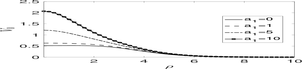
(b) $V_{0}(\rho)$ with $S=5$ for several $a_{1}$

Figure 21: Solution profiles $V_{0}(\rho)$ with different $a_{1}$ for two values of $S_{0}$, as computed numerically from (5.3). The spot height increases as the strength $a_{1}$ of the feed concentration increases.

We now use this construction to account for the spot height of the pinned spot observed in the PDE simulations shown in Fig. 19(b), in which $a_{0}=4.3$ and $a_{1}=4.2708$. For this value of $a_{0}$, (5.8) yields that $S_{0}=2.15$. Then, by computing the solution to the new core problem (5.3) with $S_{0}=2.15$ and $a_{1}=4.2708$, we find that the predicted spot height is $V_{0}(0)\approx 0.8755$. This value is very close to the spot height, given approximately by $0.8754$, observed in the full PDE simulation results shown in Fig. 19(b).

5.1.2 Linear stability analysis

Next, we analyze the linear stability of a pinned spot. We let $v_{e}$ and $u_{e}$ denote the quasi-equilibrium solution and we introduce the perturbation

$$v=v_{e}+e^{\lambda t}\phi\,,\qquad u=u_{e}+e^{\lambda t}\eta\,,$$

into (5.1) and linearize. This yields the eigenvalue problem

$$\varepsilon^{2}\Delta\phi-\phi+2u_{e}v_{e}\phi+v_{e}^{2}\eta=\lambda\phi\,,\qquad\Delta\eta-\varepsilon^{2}\left(2u_{e}v_{e}\phi+v_{e}^{2}\eta\right)=\lambda\eta\,.$$ (5.9)

To examine the possibility of locally non-radially symmetric instabilities near the spot, we let $\phi\sim e^{im\theta}\Phi_{0}(\rho)$ and $\eta\sim e^{im\theta}N_{0}(\rho)$ in (5.9) for integer modes $m\geq 2$, where $\rho=\varepsilon^{-1}|\mathbf{x}-\boldsymbol{\xi}|$. Then, upon using $v_{e}\sim V_{0}(\rho)$ and $u_{e}\sim U_{0}(\rho)$, to leading order we obtain an eigenvalue problem in the inner region

$$\Delta_{\rho}\Phi_{0}-\frac{m^{2}}{\rho^{2}}\Phi_{0}-\Phi_{0}+2U_{0}V_{0}\Phi_{0}+V_{0}^{2}N_{0}=\lambda\Phi_{0}\,,\qquad\Delta_{\rho}N_{0}-\frac{m^{2}}{\rho^{2}}N_{0}-2U_{0}V_{0}\Phi_{0}-V_{0}^{2}N_{0}=0\,,$$ (5.10)

where $\Delta_{\rho}=\partial_{\rho\rho}+\rho^{-1}\partial_{\rho}$. For the non-radially symmetric modes with $m\geq 2$, we can impose that $\Phi_{0}\to 0$ exponentially as $\rho\to\infty$ and impose the algebraic decay condition $N_{0}\sim\mathcal{O}(\rho^{-m})$ as $\rho\to\infty$. We remark that the eigenvalue problem (5.10) depends on $S_{0}$ and $a_{1}$ through the solution $V_{0}$ and $U_{0}$ to the new core problem (5.3).

By discretizing (5.10), we obtain a generalized matrix eigenvalue problem. For each mode $m\geq 2$, we numerically compute the eigenvalue $\lambda_{0}$ of the discretization of (5.10) with the largest real part as a function of $a_{1}$ and the source strength $S_{0}$. The instability threshold occurs when $\mathrm{Re}(\lambda_{0})=0$. In Fig. 22, we plot $\mathrm{Re}(\lambda_{0})$ versus $S_{0}$ for modes $m=2,3,4$ for various values of $a_{1}$. We define $\Sigma_{m}(a_{1})$ to be the spot source strength corresponding to the stability threshold $\mbox{Re}(\lambda_{0})=0$ for angular mode $m$ and concentrated feed intensity $a_{1}$. When $a_{1}=0$, where there is no concentration of the feed rate, we have from [17] (see the summary in §2.2) that there is an ordering principle $\Sigma_{2}(0)<\Sigma_{3}(0)<\Sigma_{4}(0)<\ldots$ for the mode instability thresholds. Therefore, when $a_{1}=0$, the peanut-splitting mode $m=2$ is the first mode to lose stability as $S_{0}$ is increased. However, a qualitatively new result for our pinned spot solution is that this ordering principle can be violated if the feed intensity $a_{1}$ is large enough. In particular, if $a_{1}=20$, we observe from Fig. 22(d) that $\Sigma_{3}(20)<\Sigma_{2}(20)$, which implies that the $m=3$ mode is the first to lose stability as $S_{0}$ is increased.

To illustrate this instability we compute full numerical solutions to the PDE (5.1) in the unit disk with $\varepsilon=0.03$, $a_{1}=20$, and concentrated feed rate at the origin $\boldsymbol{\xi}=(0,0)^{T}$. We choose $a_{0}=17$, and so from (5.8) with $|\Omega|=\pi$ we get $S_{0}=8.5$. From Fig. 22(d), we observe that both the $m=2$ and $m=3$ modes are unstable since $S_{0}=8.5>\Sigma_{2}(20)>\Sigma_{3}(20)$, with the $m=3$ mode having the larger positive eigenvalue. In the numerical PDE results shown in Fig. 23 at times $t=212$ and $t=231$, we observe a mode $m=3$ instability for the pinned spot that triggers a nonlinear spot-splitting process, but with ultimately only one new spot surviving by time $t=300$. However, by increasing the value of $a_{0}$ to $a_{0}=18$ and $a_{0}=19$ for which $S_{0}=9$ and $S_{0}=9.5$, we observe from Fig. 24 and Fig. 25, respectively, that the most unstable mode $m=3$ mode can trigger the creation of two or even three new spots by a nonlinear spot-splitting event.

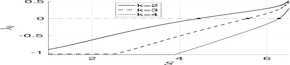
(a) $a_{1}=1$

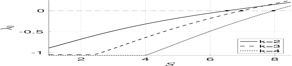
(b) $a_{1}=10$

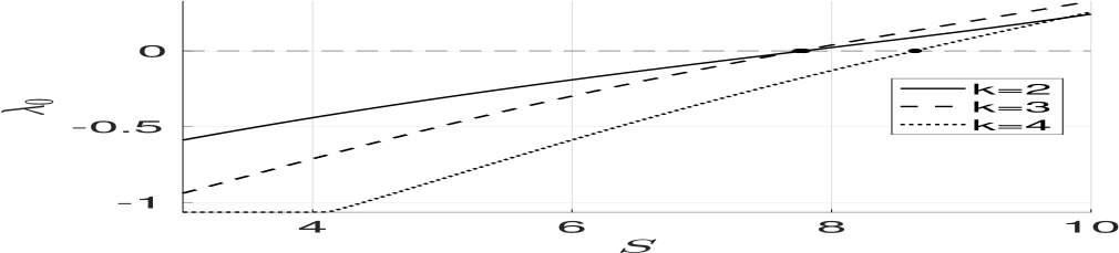
(c) $a_{1}=16$

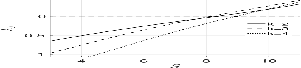
(d) $a_{1}=20$

Figure 22: Numerically computed eigenvalue $\lambda_{0}$ of (5.10) with the largest real part versus $S_{0}$ for modes $m=2,3,4$ and four different feed intensities $a_{1}$. The critical thresholds $\Sigma_{m}(a_{1})$ are the values of $S_{0}$ where $\mbox{Re}(\lambda_{0})=0$. Top left panel: $a_{1}=1$, $\Sigma_{2}(1)\approx 4.4358\,,\Sigma_{3}(1)\approx 5.5580\,,\Sigma_{4}(1)\approx 6.2736$. Top right panel: $a_{1}=10$, $\Sigma_{2}(10)\approx 6.5219\,,\Sigma_{3}(10)\approx 6.9735\,,\Sigma_{4}(10)\approx 7.9601$. Bottom left panel: $a_{1}=16$, $\Sigma_{2}(16)\approx 7.7854\,,\Sigma_{3}(16)\approx 7.7513\,,\Sigma_{4}(16)\approx 8.6443$. Bottom right panel: $a_{1}=20$, $\Sigma_{2}(20)\approx 8.3373\,,\Sigma_{3}(20)\approx 8.1346\,,\Sigma_{4}(20)\approx 8.9531$.

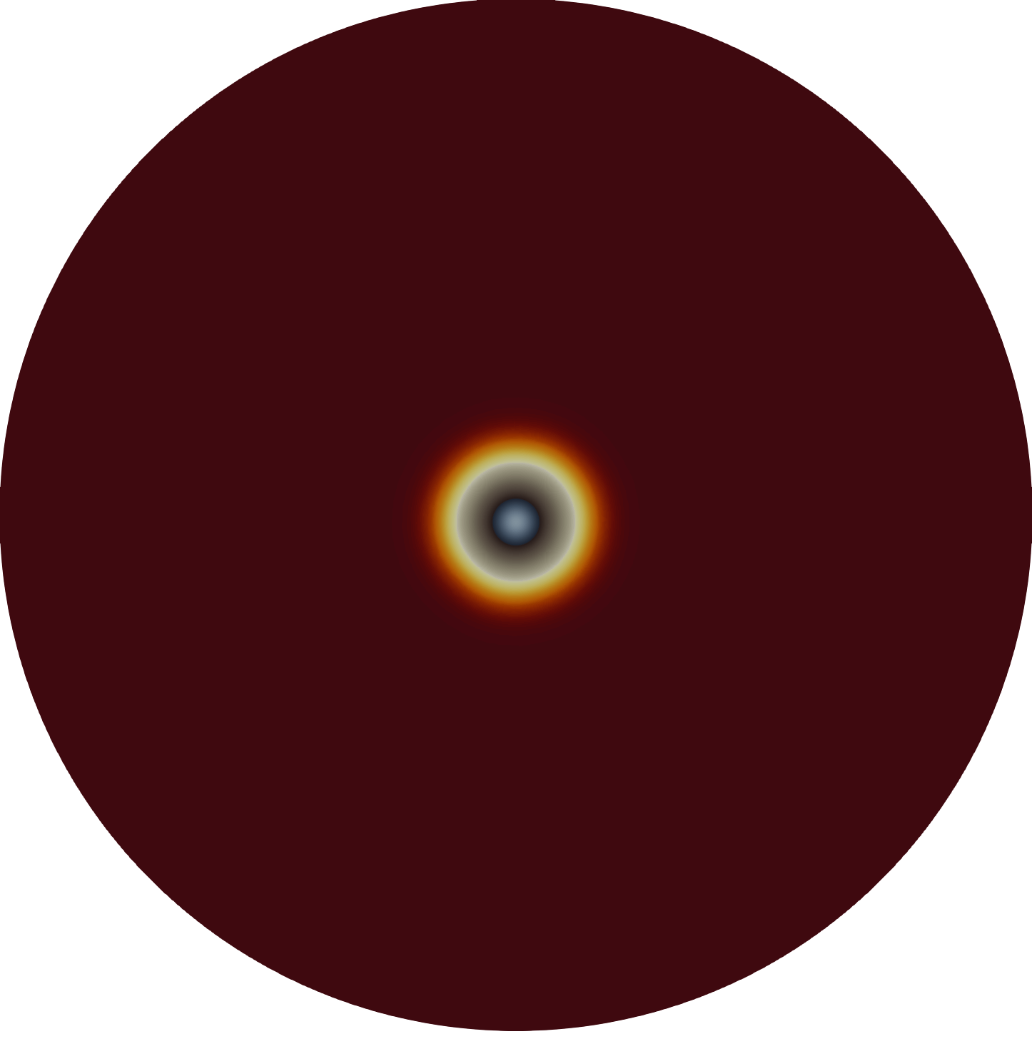
(a) $t=0$

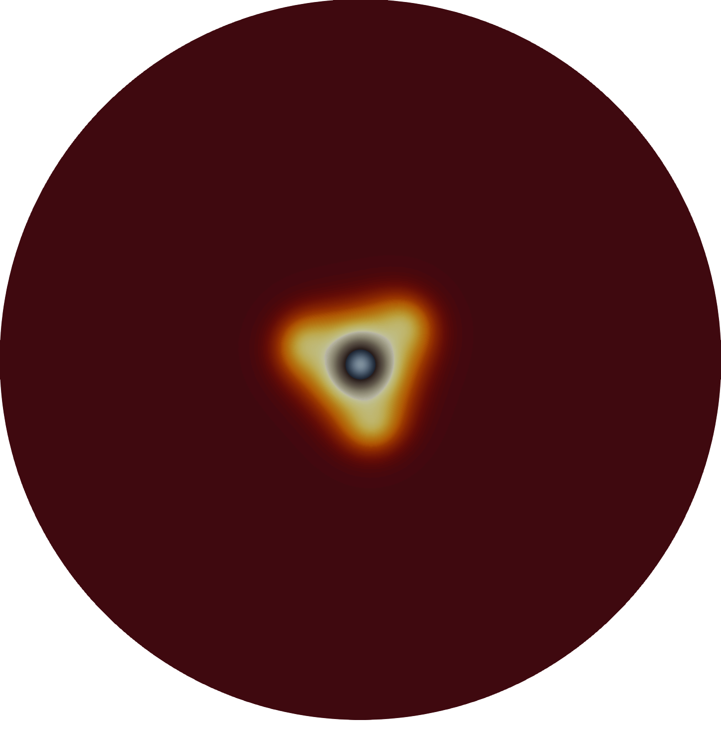
(b) $t=212$

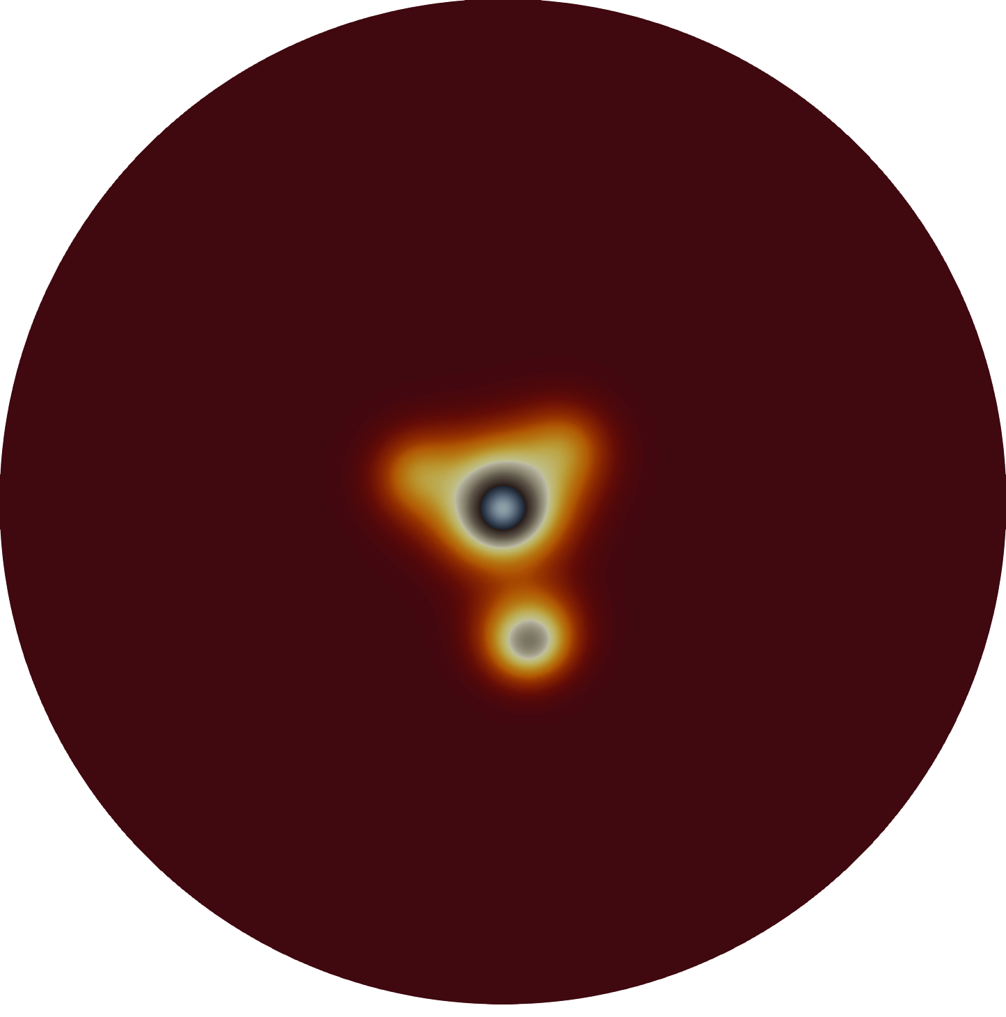
(c) $t=231$

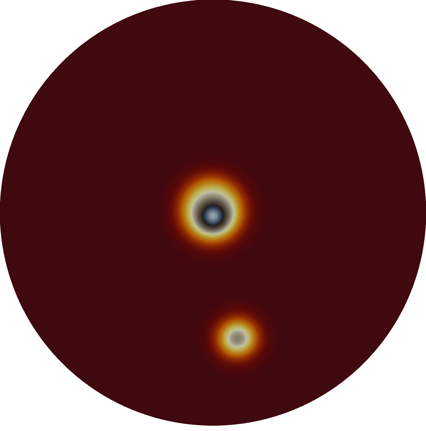
(d) $t=300$

Figure 23: PDE simulation results of (5.1) for $v$ in the unit disk with $\varepsilon=0.03$, $a_{1}=20$, and concentrated feed rate at the origin $\boldsymbol{\xi}=(0,0)$. With $a_{0}=17$ the pinned spot exhibits a mode $m=3$ instability by time $t=212$, but ultimately only one spot persists by $t=300$.

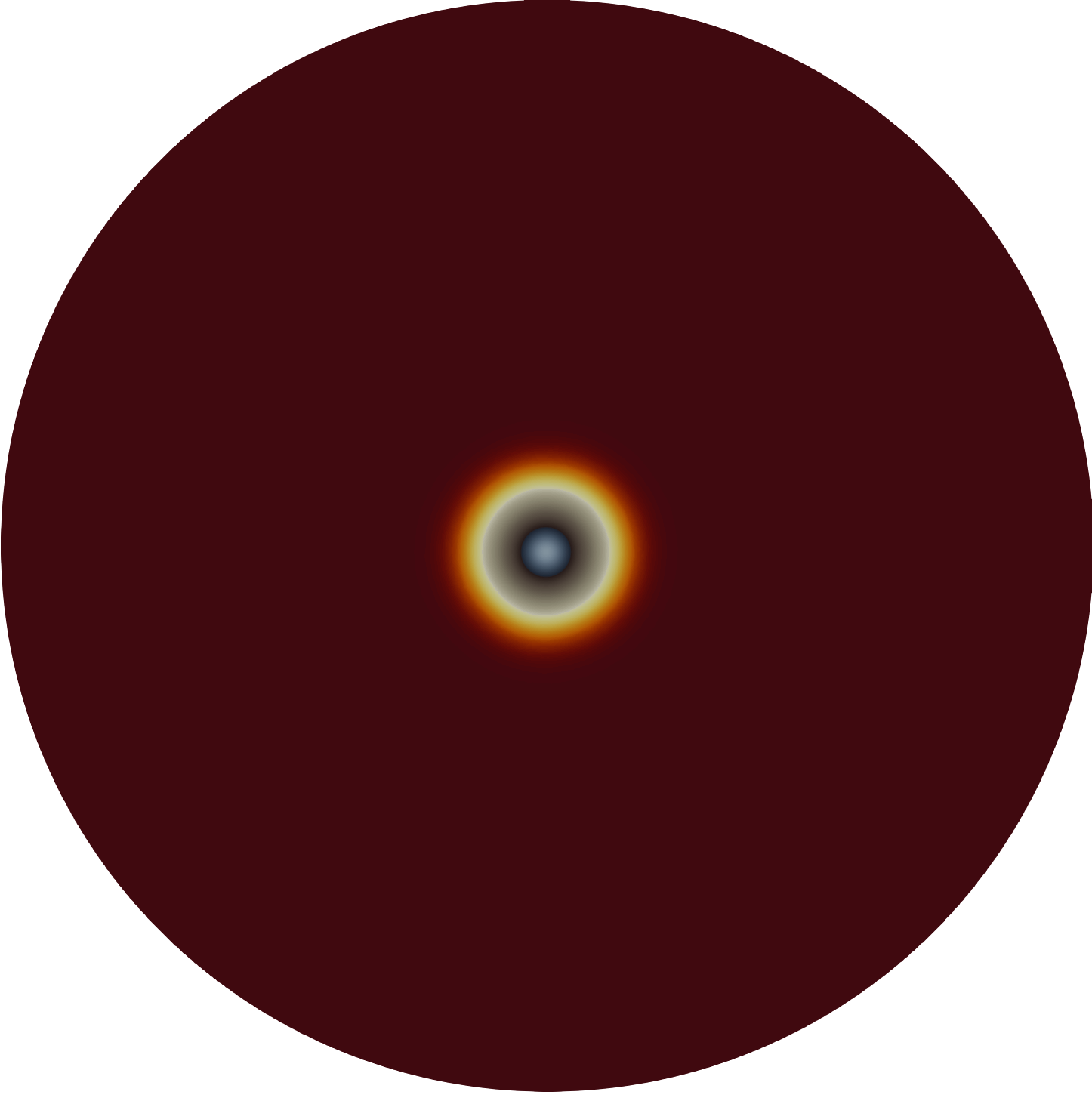
(a) $t=0$

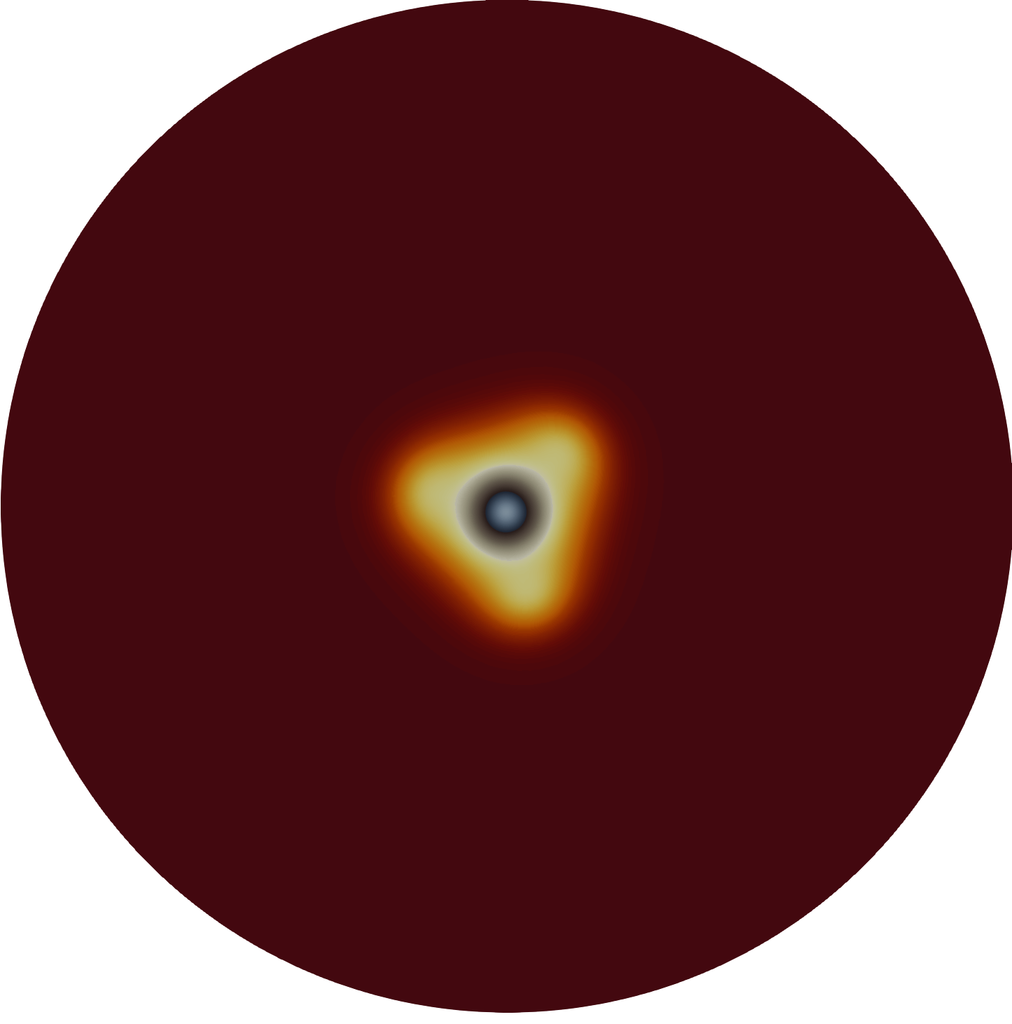
(b) $t=50$

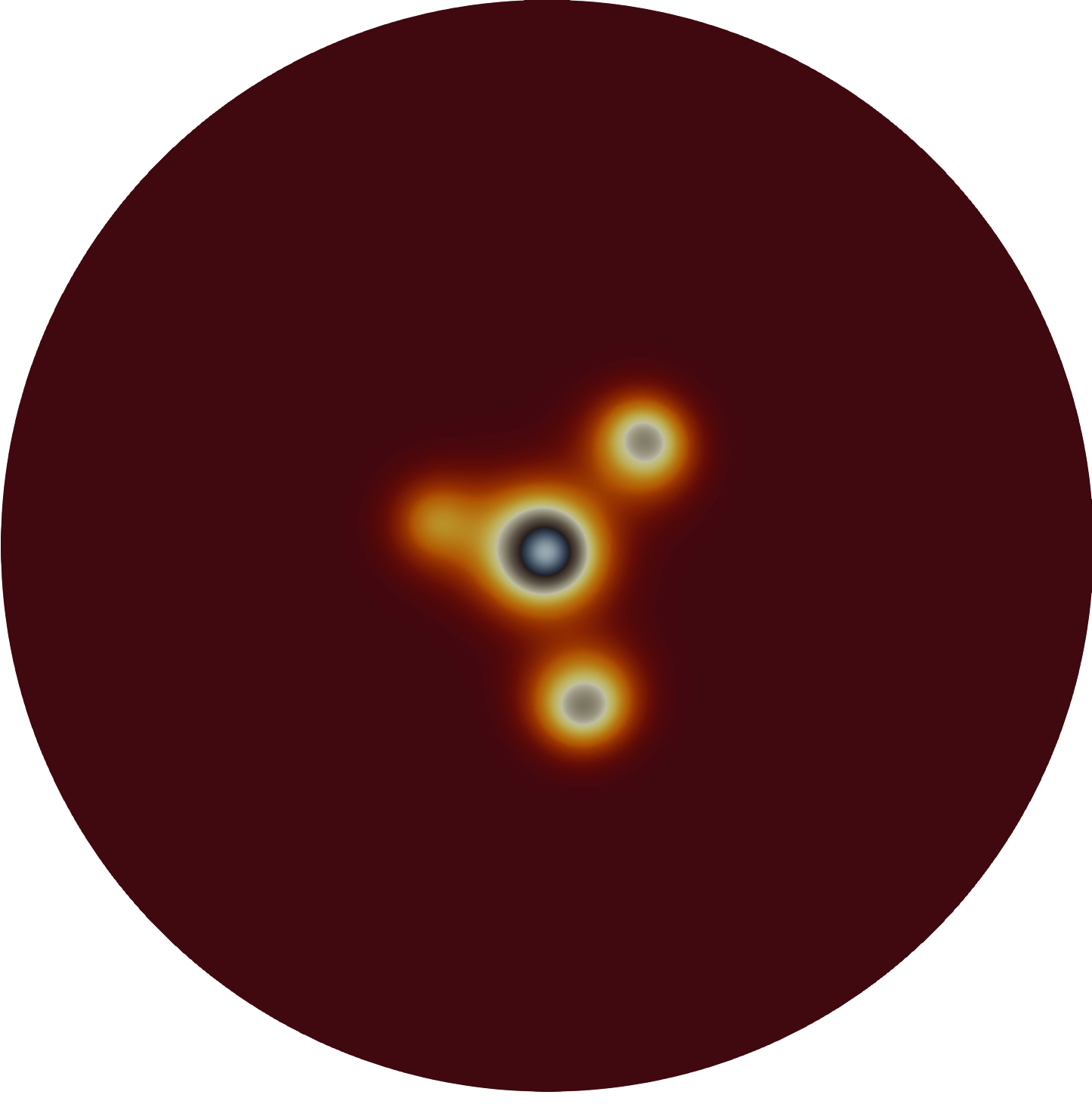
(c) $t=64$

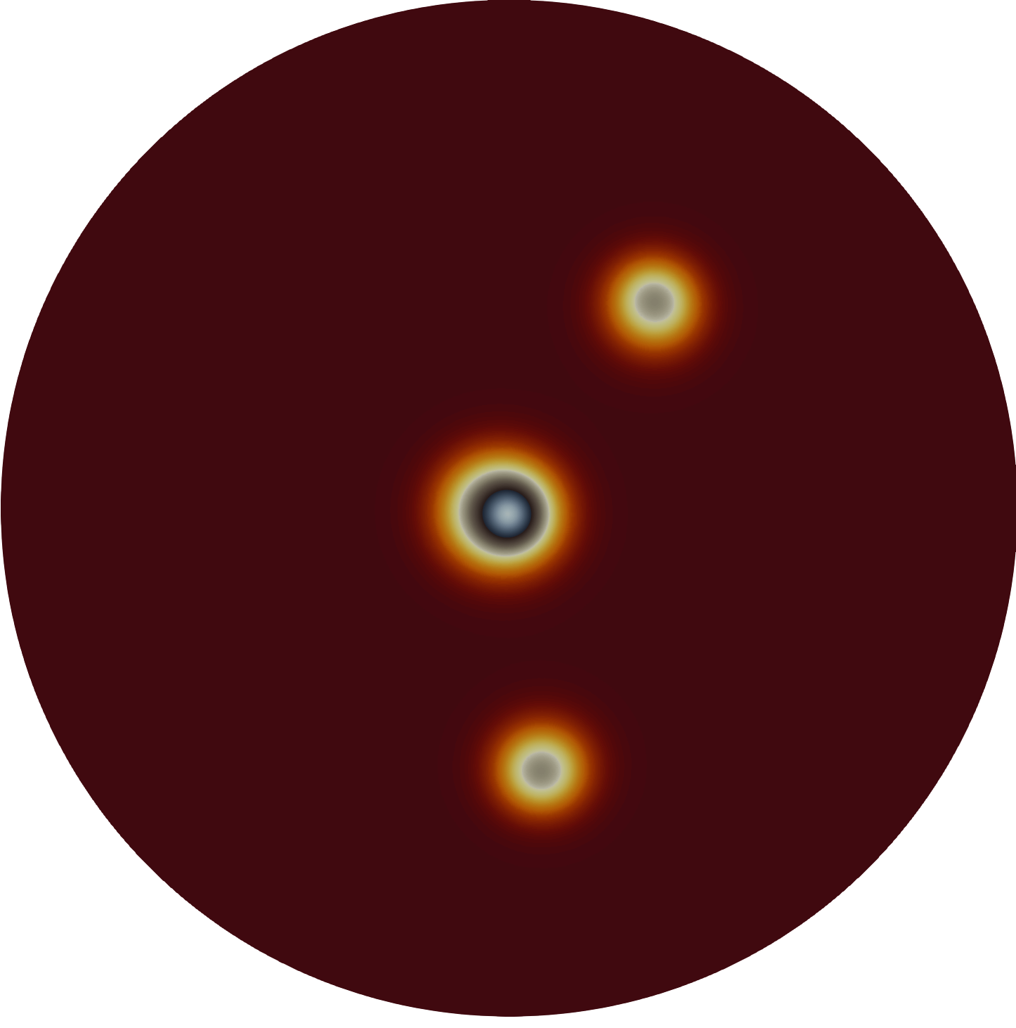
(d) $t=100$

Figure 24: Same caption as in Fig. 23 except that $a_{0}$ is increased to $a_{0}=18$. The mode $m=3$ instability of the pinned spot leads to two new spots.

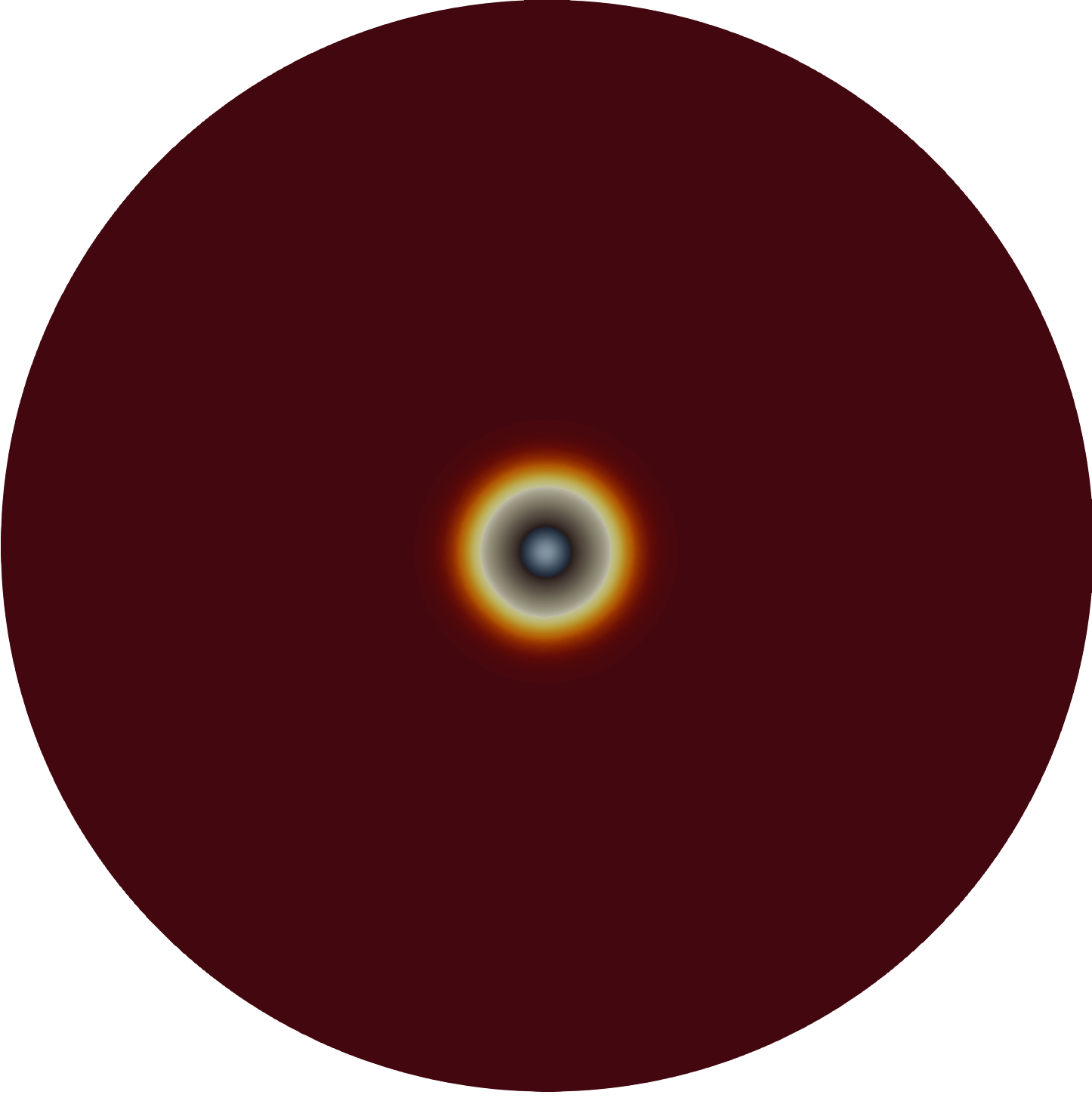
(a) $t=0$

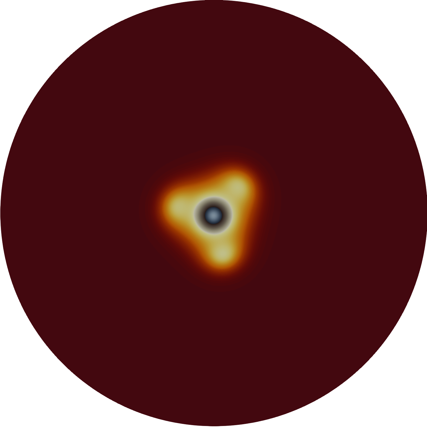
(b) $t=31$

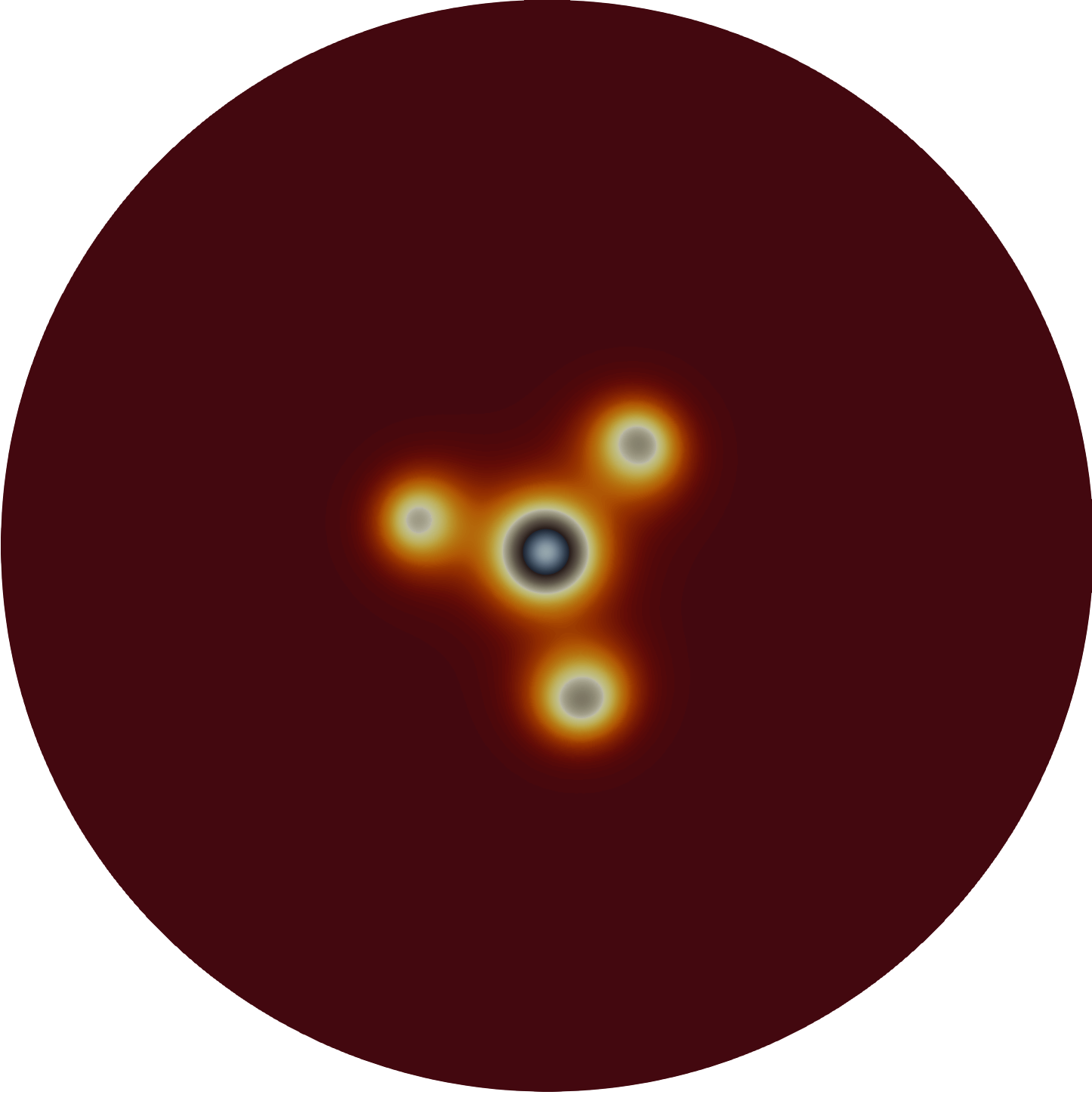
(c) $t=39$

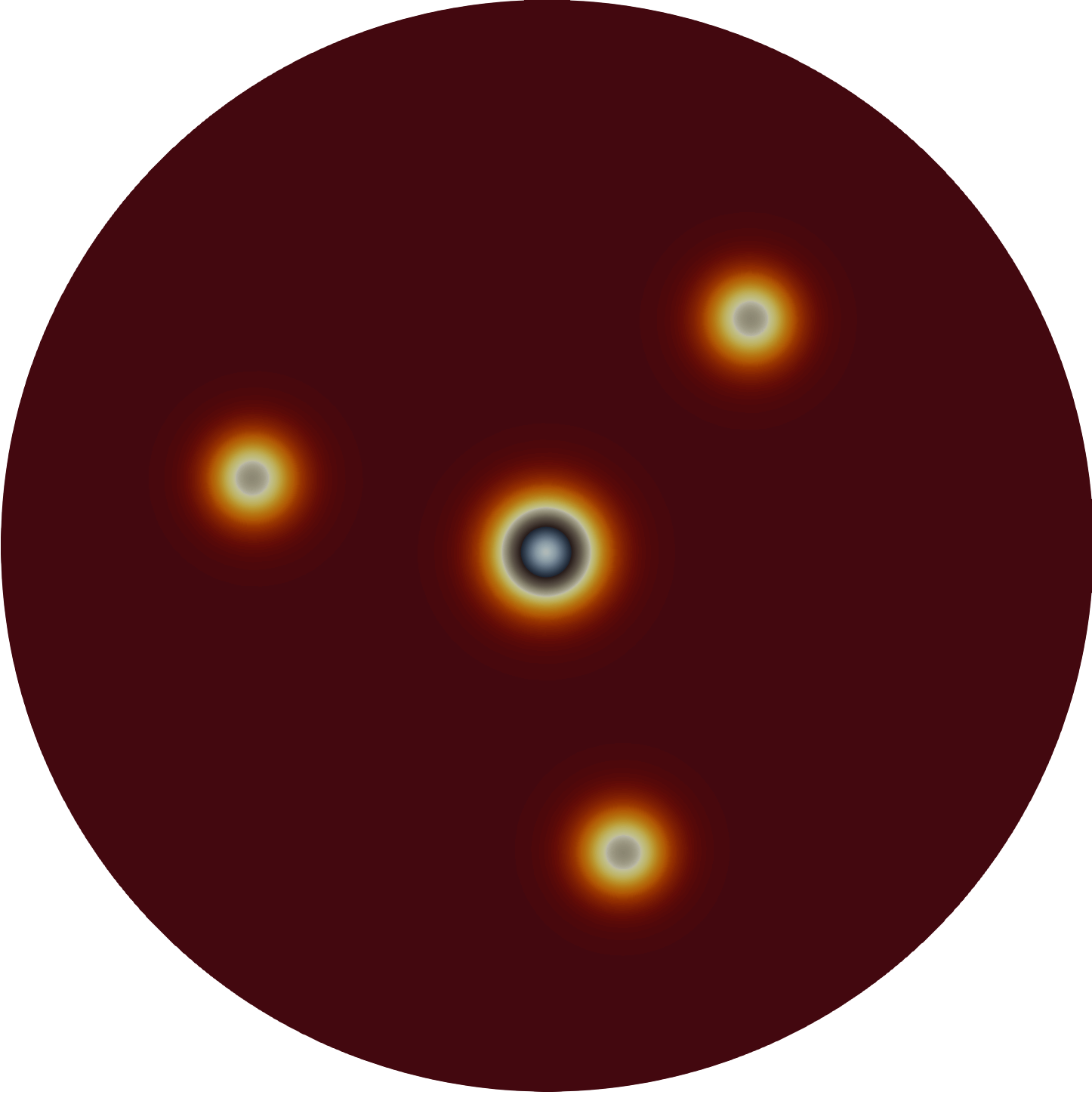
(d) $t=99$

Figure 25: Same caption as in Fig. 23 except that $a_{0}$ is increased further to $a_{0}=19$. The mode $m=3$ instability of the pinned spot now leads to three new spots.

5.1.3 Effect of a moving localized feed-rate

We have shown in §4.1.1 from the ODE (4.16) for slow spot dynamics that when a spot is close enough to the concentration point $\boldsymbol{\xi}$ for the feed rate, it will get pinned to $\boldsymbol{\xi}$ in finite time. This suggests that if the concentration point $\boldsymbol{\xi}$ is moving with time, the spot will pursue $\boldsymbol{\xi}$ and remain pinned, provided that the dynamics of $\boldsymbol{\xi}$ is slow enough. To examine this conjecture, we perform a full PDE simulation of (5.1) for $a_{1}=8$, $a_{0}=5$, and $\boldsymbol{\xi}=\boldsymbol{\xi}(\varepsilon^{2}t)$ with $\varepsilon=0.03$, where we choose

$$\boldsymbol{\xi}=(\xi_{1},\xi_{2})^{T}\,,\quad\xi_{1}=0.5\cos(2\pi\varepsilon^{2}t)\,,\quad\xi_{2}=0.5\sin(2\pi\varepsilon^{2}t)\,.$$ (5.11)

In Fig. 26 we show that the trajectory of the pinned spot aligns closely with the motion of the rotating concentration point $\boldsymbol{\xi}(\varepsilon^{2}t)$. This supports the conjecture that a spot will follow the trajectory of the concentration point of the feed rate.

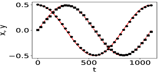
Figure 26: The concentration point for the feed is rotating on the ring $\boldsymbol{\xi}=(\xi_{1}(t),\xi_{2}(t))^{T}=0.5(\cos(2\pi\varepsilon^{2}t),\sin(2\pi\varepsilon^{2}t))^{T}$ with $\varepsilon=0.03$, and we choose $a_{0}=5$ and $a_{1}=8$. The $x$ and $y$ coordinates of the pinned spot, as computed numerically from the full PDE (5.1), are shown by the black dots and square, respectively. We observe a close agreement between the spot coordinates and the coordinates $\xi_{1}(t)$ (solid line) and $\xi_{2}(t)$ (dashed line) of the concentration point $\boldsymbol{\xi}$ of the feed rate.

5.2 Quasi-equilibrium spot patterns with a pinned spot

In this subsection we analyze the slow dynamics and linear stability of quasi-equilibrium spot patterns that have a pinned spot, such as shown in Fig. 23–25.

5.2.1 Quasi-equilibria and slow spot dynamics

We construct a quasi-equilibrium spot pattern, with $N$ spots centered at $\mathbf{x}_{j}\in\Omega$ for $j=1,\ldots,N$, and with an additional pinned spot at the concentration point $\boldsymbol{\xi}\in\Omega$ of the feed rate. We assume that the spots and the pinned-spot are well-separated in the sense that

$$|\mathbf{x}_{i}-\mathbf{x}_{j}|=\mathcal{O}(1)\,,\quad i\neq j\,,\qquad|\mathbf{x}_{i}-\boldsymbol{\xi}|=\mathcal{O}(1)\,,\quad i=1,\ldots,N\,.$$ (5.12)

Near the $j^{\text{th}}$ spot centered at $\mathbf{x}_{j}$, for $j=1,\ldots,N$, we substitute the expansion (2.1) with $D=1$ into (5.1). Due to the assumption (5.12), the term $\Phi\left(|\mathbf{x}_{j}-\boldsymbol{\xi}|/\varepsilon\right)$ is exponentially small as $\varepsilon\to 0$, and therefore absent to all algebraic orders in $\varepsilon$. We retrieve the core problem (2.2) and the integration identity (2.4). Likewise, near the the pinned spot at $\boldsymbol{\xi}$, we substitute $v\sim V_{0}(\rho)$ and $u\sim U_{0}(\rho)$ into (5.1) to obtain the new core problem (5.3). Upon using the distributional limits (2.5) (with $D=1$) and (5.5), the outer problem for $u$, defined away from all the spots, is

$$\Delta u+a_{0}-2\pi\sum\limits_{i=1}^{N}S_{i}\,\delta(\mathbf{x}-\mathbf{x}_{j})-2\pi S_{0}\,\delta(\mathbf{x}-\boldsymbol{\xi})=0\,,\quad\mbox{in}\quad\Omega\,,\qquad\partial_{n}u=0\,,\quad\mbox{on}\quad\partial\Omega\,.$$ (5.13)

In terms of the Neumann Green’s function of (2.9), the solution to (5.13) is

$$u=-2\pi S_{0}\,G(\mathbf{x};\boldsymbol{\xi})-2\pi\sum\limits_{i=1}^{N}S_{i}\,G(\mathbf{x};\mathbf{x}_{i})+\bar{u}\,,$$ (5.14)

where $\bar{u}$ is an undetermined constant. By using the divergence theorem on (5.13), we conclude that

$$\sum\limits_{i=0}^{N}S_{i}={a_{0}|\Omega|/(2\pi)}\,.$$ (5.15)

Next, we let $\mathbf{x}\to\mathbf{x}_{j}$, for $j=1,\ldots,N$, in (5.14) to obtain that

$$\begin{split}u&\sim S_{j}\log|\mathbf{x}-\mathbf{x}_{j}|-2\pi\left(S_{j}R_{j,j}+S_{0}G(\mathbf{x}_{j};\boldsymbol{\xi})+\sum_{i\neq j}^{N}S_{i}\,G_{j,i}\right)+\bar{u}\\ &\quad-2\pi\left(S_{j}\nabla_{\mathbf{x}}R_{j,j}+S_{0}\nabla_{\mathbf{x}}G(\mathbf{x}_{j};\boldsymbol{\xi})+\sum_{i\neq j}^{N}S_{i}\nabla_{\mathbf{x}}G_{j,i}\right)\cdot(\mathbf{x}-\mathbf{x}_{j})+{\mathcal{O}}(|\mathbf{x}-\mathbf{x}_{j}|^{2})\,,\qquad j=1,\ldots,N\,,\end{split}$$ (5.16)

where $R_{j,j}\equiv R(\mathbf{x}_{j};\mathbf{x}_{j})$ and $G_{j,i}\equiv G(\mathbf{x}_{j};\mathbf{x}_{i})$. Upon matching the ${\mathcal{O}}(1)$ terms in (5.16) with the far-field behavior (2.2b) of the leading order core solution, we find that

$$S_{j}+2\pi\nu\left(S_{j}R_{j,j}+S_{0}G(\mathbf{x}_{j};\boldsymbol{\xi})+\sum\limits_{i\neq j}^{N}S_{i}\,G_{j,i}\right)+\nu\chi(S_{j})=\nu\bar{u}\,,\qquad j=1\,,\ldots,N\,.$$ (5.17)

Then, we expand (5.14) as $\mathbf{x}\to\boldsymbol{\xi}$ to get

$$u\sim S_{0}\log|\mathbf{x}-\boldsymbol{\xi}|-2\pi S_{0}\,R_{0,0}-2\pi\sum\limits_{i=1}^{N}S_{i}\,G_{j,0}+\bar{u}+{\mathcal{O}}(|\mathbf{x}-\mathbf{x}_{j}|)\,,$$ (5.18)

where $R_{0,0}\equiv R(\boldsymbol{\xi};\boldsymbol{\xi})$ and $G_{j,0}\equiv G(\mathbf{x}_{j};\boldsymbol{\xi})$. Upon matching (5.18) with the far-field behavior (5.3b) of the new core problem, we conclude that

$$S_{0}+2\pi\nu\left(S_{0}R_{0,0}+\sum\limits_{i=1}^{N}S_{i}\,G_{j,0}\right)+\nu\chi(S_{0};a_{1})=\nu\bar{u}\,,$$ (5.19)

Next, we write (5.17), (5.19), and (5.15) in matrix form as

$$\mathbf{s}+2\pi\nu\,\mathcal{G}\mathbf{s}+\nu\,\boldsymbol{\chi}=\nu\bar{u}\,\mathbf{e}\,,\qquad\mathbf{e}^{T}\mathbf{s}=p_{a}\equiv\frac{a_{0}|\Omega|}{2\pi}\,,$$ (5.20a)

where we have defined

$$\mathbf{s}\equiv(S_{0},S_{1},\ldots,S_{N})^{T}\,,\qquad\bm{\chi}\equiv\left(\chi(S_{0};a_{1}),\chi(S_{1}),\ldots,\chi(S_{N})\right)^{T}\,,\qquad\mathbf{e}\equiv(1,\ldots,1)^{T}\in\mathbb{R}^{N+1}\,.$$ (5.20b)

Here $\chi(S_{0};a_{1})$ is defined by the new core problem (5.3) for the pinned spot, while $\mathcal{G}\in\mathbb{R}^{(N+1)\times(N+1)}$ is the Neumann Green’s matrix of $\boldsymbol{\xi},\mathbf{x_{1}},\ldots,\mathbf{x}_{N}$. Upon eliminating $\bar{u}$ in (5.20b), we obtain that the nonlinear algebraic system for the vector $\mathbf{s}$ of source strengths is

$$\mathbf{s}+2\pi\nu(\mathcal{I}-\mathcal{E})\mathcal{G}\mathbf{s}+\nu(\mathcal{I}-\mathcal{E})\boldsymbol{\chi}=\frac{p_{a}}{N+1}\mathbf{e}\,,\qquad\mbox{with}\qquad\bar{u}=\frac{p_{a}+2\pi\nu\,\mathbf{e}^{T}\mathcal{G}\mathbf{s}+\nu\,\mathbf{e}^{T}\boldsymbol{\chi}}{\nu(N+1)}\,.$$ (5.21)

Here $\mathcal{E}=N^{-1}\mathbf{e}\mathbf{e}^{T}\in\mathbb{R}^{(N+1)\times(N+1)}$ and $\mathcal{I}\in\mathbb{R}^{(N+1)\times(N+1)}$ is the identity matrix.

To derive the DAE system for slow spot dynamics we must match (2.10) (setting $D=1$) with (5.16) for the $\mathcal{O}(\varepsilon)$ gradient terms. This matching condition yields the far-field behavior for the inner correction term $U_{j1}$ in (2.1):

$$U_{j1}\sim-2\pi\left[S_{j}\nabla_{\mathbf{x}}R_{j,j}+\sum\limits_{i\neq j}^{N}S_{i}\nabla_{\mathbf{x}}G_{j,i}+S_{0}\nabla_{\mathbf{x}}G(\mathbf{x}_{j};\boldsymbol{\xi})\right]\cdot\mathbf{y}\,\qquad\mbox{as}\quad|\mathbf{y}|\to\infty\,,$$ (5.22)

where $\mathbf{y}=\varepsilon^{-1}(\mathbf{x}-\mathbf{x}_{j})$. Following the derivation in §2.1, we obtain that the DAE system for slow spot dynamics is

$$\frac{d\mathbf{x}_{j}}{d\sigma}=-\gamma(S_{j})\left(\,\boldsymbol{\beta}_{j}+2\pi S_{0}\nabla_{\mathbf{x}}G(\mathbf{x}_{j};\boldsymbol{\xi})\right)\,,\qquad j=1,\ldots,N\,,$$ (5.23)

where $\sigma=\varepsilon^{2}t$. Here, $\boldsymbol{\beta}_{j}$ and $\gamma(S_{j})$ are defined in (2.12) and (2.18), respectively, while $\mathbf{s}\equiv(S_{0},S_{1},\ldots,S_{N})^{T}$ satisfies the nonlinear algebraic system (5.21).

We now compare the DAE dynamics (5.23) and (5.21) with full numerical results computed from the PDE (5.1) in the unit disk. We set $\varepsilon=0.03$, and for the localized feed rate we choose $a_{0}=15$, $a_{1}=5$, and $\boldsymbol{\xi}=\mathbf{0}$. The initial quasi-equilibrium pattern has a pinned spot at the origin $\boldsymbol{\xi}=\mathbf{0}$, and two additional spots centered at $(0.5,0)^{T}$ and $(0,0.5)^{T}$. As shown in Fig. 27(c), the pinned spot remains at the origin while the other two spots move apart to form an almost colinear pattern. The spot trajectories computed from the full PDE simulation agree well with those from the DAE system.

(a) x-coordinate

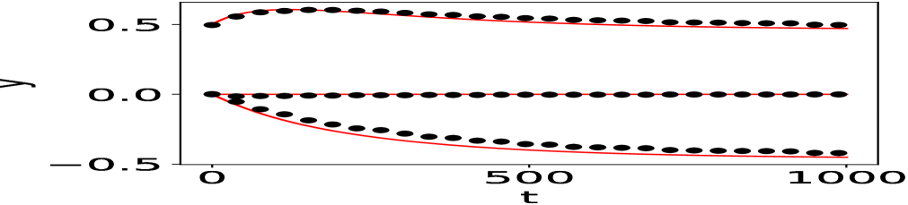
(b) y-coordinate

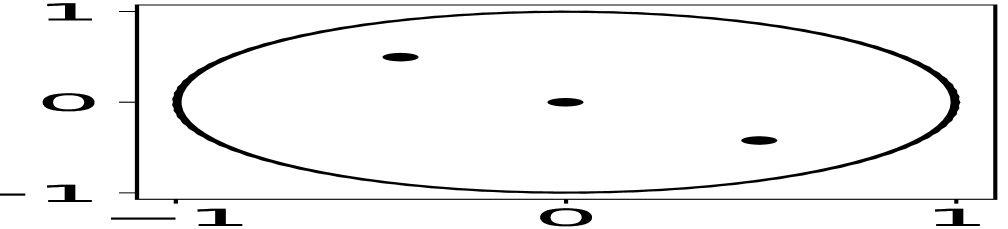
(c) $t=1000$

Figure 27: Left and middle panels: The spot trajectories for an initial quasi-equilibrium pattern with spots centered at $(0.5,0.0)^{T}$ and $(0.0,0.5)^{T}$, and with a pinned spot centered at the origin $\boldsymbol{\xi}=\mathbf{0}$. The full PDE results from (5.1) and DAE dynamics (5.23) and (5.21) are represented by the black dots and red solid line, respectively. Right panel: spot locations at $t=1000$ form a colinear pattern (near the steady-state). Parameters are $\varepsilon=0.03$, $a_{0}=15$, and $a_{1}=5$.

For our second experiment in the unit disk, we set $\varepsilon=0.03$ and consider a localized feed rate with $a_{0}=10$ and $a_{1}=5$, where the concentration point $\boldsymbol{\xi}$ moves slowly in time according to (5.11). At time $t=0$ the quasi-equilibrium pattern consists of the pinned spot centered at $\boldsymbol{\xi}(0)=(0.5,0)^{T}$ with an additional spot centered at $(-0.5,0)^{T}$. In Fig. 28 we show a favorable comparison between the spot trajectories obtained from the DAE dynamics (5.23) and (5.21) and from the full PDE computations of (5.1) on $0<t<1000$. We observe that the initial pinned-spot remains pinned as time increases and moves with $\boldsymbol{\xi}(t)$ along a circular trajectory. The other spot moves along a nearly circular trajectory in the unit disk.

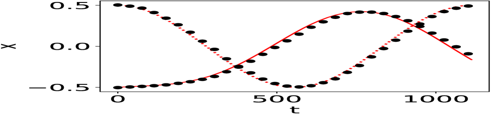
(a) x-coordinate

(b) y-coordinate

Figure 28: A two-spot quasi-equilibrium pattern with the moving concentration point $\boldsymbol{\xi}(\varepsilon^{2}t)$ of the feed rate given in (5.11), and with $\varepsilon=0.03$, $a_{0}=10$, and $a_{1}=5$. At time $t=0$, there is a pinned spot centered at $\boldsymbol{\xi}(0)=(0.5,0.0)^{T}$ and an additional spot at $(-0.5,0.0)^{T}$. The solid red curve is the spot trajectory from the DAE dynamics (5.23) and (5.21). The dashed red curve is the moving concentration point $\boldsymbol{\xi}(\varepsilon^{2}t)$. The black dots are the locations of the spot and pinned-spot, as computed numerically from the PDE (5.1).

5.2.2 Linear stability analysis

We now analyze the linear stability of a quasi-equilibrium pattern $v_{e}$ and $u_{e}$ that consists of spots centered at $\mathbf{x}_{1},\ldots,\mathbf{x}_{N}$ with an additional pinned spot at $\boldsymbol{\xi}$, for which the source strengths are $S_{1},\ldots,S_{N}$ and $S_{0}$, respectively. For instabilities associated with non-radially symmetric perturbations near the spots, our previous results in §2.2 and §5.1.2 have shown that the quasi-equilibrium pattern is linearly stable to symmetry breaking bifurcations in the spot profiles only when

$$S_{j}<\Sigma_{2}(0)\approx 4.302\,,\quad\mbox{for}\quad j=1,\ldots,N\qquad\mbox{and}\qquad S_{0}<\min_{m\geq 2}\Sigma_{m}(a_{1})\,.$$ (5.24)

Here the symmetry-breaking stability threshold $\Sigma_{m}(a_{1})$ for the local angular mode $m$ was defined in §5.1.2 (see Fig. 22).

As such, we will focus only on deriving a new GCEP associated with any instabilities due to locally radiallly symmetric perturbations near the spots. Upon substituting $v=v_{e}+e^{\lambda t}\phi$ and $u=u_{e}+e^{\lambda t}\eta$ into (5.1), we linearize to get

$$\varepsilon^{2}\Delta\phi-\phi+2u_{e}v_{e}\phi+v_{e}^{2}\eta=\lambda\phi\,,\qquad\Delta\eta-\varepsilon^{-2}\left(2u_{e}v_{e}\phi+v_{e}^{2}\eta\right)=\lambda\eta\,,\quad\mbox{in}\quad\Omega\,,$$ (5.25)

with $\partial_{n}\phi=\partial_{n}\eta=0$ on $\partial\Omega$. From the leading-order construction of the quasi-equilibrium pattern in §5.2.1, we have that

$$v_{e}\sim\begin{cases}V_{0}\left(\varepsilon^{-1}|\mathbf{x}-\boldsymbol{\xi}|\right)\,,&\quad\mbox{near}\,\,\boldsymbol{\xi}\,,\\[3.0pt] V_{j0}\left(\varepsilon^{-1}|\mathbf{x}-\mathbf{x}_{j}|\right)\,,&\quad\mbox{near}\,\,\mathbf{x}_{j}\,,\end{cases}\qquad\mbox{and}\qquad u_{e}\sim\begin{cases}U_{0}\left(\varepsilon^{-1}|\mathbf{x}-\boldsymbol{\xi}|\right)\,,&\quad\mbox{near}\,\,\boldsymbol{\xi}\,,\\[3.0pt] U_{j0}\left(\varepsilon^{-1}|\mathbf{x}-\mathbf{x}_{j}|\right)\,,&\quad\mbox{near}\,\,\mathbf{x}_{j}\,,\end{cases}$$ (5.26)

Here $(V_{j0},U_{j0})$ is the solution to the core problem (2.2) while $(V_{0},U_{0})$ is the solution to the new core problem (5.3) near the pinned spot, which depends on the feed intensity parameter $a_{1}$.

In the inner region near a spot at $\mathbf{x}_{j}$, for $j=1,\ldots,N$, we let $\phi\sim c_{j}\tilde{\Phi}_{j}(\rho)$ and $\eta\sim c_{j}\tilde{N}_{j}(\rho)$ in (5.25), where $\rho=\varepsilon^{-1}|\mathbf{x}-\mathbf{x}_{j}|$. Upon using (5.26), we retrieve the inner problem (2.22) for $\tilde{\Phi}_{j}$ and $\tilde{N}_{j}$ for each $j=1,\ldots,N$. Similarly, by setting $\phi\sim c_{0}\tilde{\Phi}_{0}(\rho)$ and $\eta\sim c_{0}\tilde{N}_{0}(\rho)$ in (5.25), where $\rho=\varepsilon^{-1}|\mathbf{x}-\boldsymbol{\xi}|$, we obtain the following inner problem for the pinned spot:

$$\Delta_{\rho}\hat{\Phi}_{0} -\hat{\Phi}_{0}+2U_{0}V_{0}\hat{\Phi}_{0}+V_{0}^{2}\hat{N}_{0}=\lambda\hat{\Phi}_{0}\,,\qquad\Delta_{\rho}\hat{N}_{0}-2U_{0}V_{0}\hat{\Phi}_{0}-V_{0}^{2}\hat{N}_{0}=0\,,\quad\rho>0\,,$$ (5.27a)

$$\hat{\Phi}_{0}^{\prime}(0)=\hat{N}_{0}^{\prime}(0)=0\,;\qquad\hat{\Phi}_{0}\to 0\,,\quad\hat{N}_{0}\sim\log\rho+\tilde{B}(S_{j};a_{1},\lambda)+o(1)\,,\quad\mbox{as}\quad\rho\to\infty\,.$$ (5.27b)

Here $\tilde{B}(S_{j};a_{1},\lambda)$ depends on the feed intensity $a_{1}$ through the pinned core solution $(V_{0},U_{0})$. By differentiating (5.3) with respect to $S_{0}$, and then comparing the resulting system with (5.27) when $\lambda=0$, we identify $\tilde{B}(S_{0};a_{1},0)=\partial_{S_{0}}\chi(S_{0};a_{1})$.

As in §2.2, to formulate the outer problem for $\eta$ we first derive the distributional limit

$$\varepsilon^{-2}\left(2u_{e}v_{e}\phi+v_{e}^{2}\eta\right)\to 2\pi c_{0}\,\delta(\mathbf{x}-\boldsymbol{\xi})+2\pi\sum\limits_{i=1}^{N}c_{i}\,\delta(\mathbf{x}-\mathbf{x}_{i})\,,$$

as $\varepsilon\to 0$. By using this limit in (5.25), and by enforcing the asymptotic matching condition to the inner solutions near the spots, we obtain that the outer problem for $\eta$, defined away from the spots, is

$$\Delta\eta- \lambda\eta-2\pi\left[\,\sum\limits_{i=1}^{N}c_{i}\,\delta(\mathbf{x}-\mathbf{x}_{i})+c_{0}\,\delta(\mathbf{x}-\boldsymbol{\xi})\,\right]=0\quad\mbox{in}\quad\Omega\,,\qquad\partial_{n}\eta=0\quad\mbox{on}\quad\partial\Omega\,.$$ (5.28a)

$$\eta \sim c_{0}\left(\log|\mathbf{x}-\boldsymbol{\xi}|+{1/\nu}+\tilde{B}(S_{0};a_{1},\lambda)\right)\,,\quad\mbox{as}\quad\mathbf{x}\to\boldsymbol{\xi}\,,$$ (5.28b)

$$\eta \sim c_{j}\left(\log|\mathbf{x}-\mathbf{x}_{j}|+{1/\nu}+\tilde{B}(S_{j};\lambda)\right)\,,\quad\mbox{as}\quad\mathbf{x}\to\mathbf{x}_{j}\,,\quad j=1,\ldots,N\,.$$ (5.28c)

For $\lambda\neq 0$, the solution to (5.28a) is represented as

$$\eta=-2\pi c_{0}\,G_{\lambda}(\mathbf{x};\boldsymbol{\xi})-2\pi\,\sum\limits_{i=1}^{N}c_{i}\,G_{\lambda}(\mathbf{x};\mathbf{x}_{i})\,,$$ (5.29)

where $G_{\lambda}$ is the eigenvalue-dependent Green’s function defined by (2.27). By matching the near-field behavior of (5.29) as $\mathbf{x}\to\boldsymbol{\xi}$ and as $\mathbf{x}\to\mathbf{x}_{j}$, for $j=1,\ldots,N$, to the required singularity behavior in (5.28b) and (5.28c), respectively, we derive a new GCEP for $\mathbf{c}\equiv(c_{0},c_{1},\ldots,c_{N})^{T}$, which we write in matrix form as

$$\mathcal{M}\mathbf{c}\equiv\mathbf{0}\qquad\mbox{where}\qquad\mathcal{M}\equiv\mathcal{I}+2\pi\nu\mathcal{G}_{\lambda}+\nu\tilde{\mathcal{B}}\,.$$ (5.30a)

Here the entries of the Green’s matrix $$\mathcal{G}_{\lambda}\in\mathbb{R}^{(N+1)\times(N+1)} \tilde{\mathcal{B}}\in\mathbb{R}^{(N+1)\times(N+1)}$$ and the diagonal matrix are given by

$$\begin{split}\left(\mathcal{G}_{\lambda}\right)_{i+1\,j+1}&=\begin{cases}G_{\lambda}(\mathbf{x}_{i};\mathbf{x}_{j})\quad&i\neq j\,,\\ R_{\lambda}(\mathbf{x}_{j};\mathbf{x}_{j})\quad&i=j\,,\end{cases}\qquad\mbox{for}\quad i,j=0,\ldots,N\,,\\ (\tilde{\mathcal{B}})_{1\,1}&=\tilde{B}(S_{0};a_{1},\lambda)\,,\qquad(\tilde{\mathcal{B}})_{j+1\,j+1}=\tilde{B}(S_{j};\lambda)\,,\quad\mbox{for}\quad j=1,\ldots,N\,,\end{split}$$ (5.30b)

where, for convenience of notation, we have defined $\mathbf{x}_{0}\equiv\boldsymbol{\xi}$. We conclude that the $N$-spot quasi-equilibrium solution with an additional pinned spot at $\boldsymbol{\xi}$ is linearly stable on ${\mathcal{O}}(1)$ time-scales to locally radially symmetric perturbations near the spots when there is no root in $\mbox{Re}(\lambda)>0$ to

$$\det\mathcal{M}(\lambda)=0\,.$$ (5.31)

Next, we formulate the GCEP for zero-eigenvalue crossings where $\lambda=0$ in (5.28). For $\lambda=0$, the solution to (5.28a) is

$$\eta=-2\pi c_{0}\,G(\mathbf{x};\boldsymbol{\xi})-2\pi\sum\limits_{i=1}^{N}c_{i}\,G(\mathbf{x};\mathbf{x}_{j})+\bar{\eta}\,,$$ (5.32)

where $G$ is the Neumann Green’s function of (2.9), and $\bar{\eta}$ is an undetermined additive constant. By applying the divergence theorem to (5.28a) we obtain that $\mathbf{e}^{T}\mathbf{c}=0$. Then, by matching the near-field behavior of (5.32) as $\mathbf{x}\to\boldsymbol{\xi}$ and as $\mathbf{x}\to\mathbf{x}_{j}$, for $j=1,\ldots,N$, to the required singularity behavior in (5.28b) and (5.28c), respectively, and by recalling the identities $\tilde{B}(S_{0};a_{1},0)=\partial_{S_{0}}\chi(S_{0};a_{1})$ and $\tilde{B}(S_{j};0)=\chi^{\prime}(S_{j})$, we obtain in matrix form that

$$\left(\,\mathcal{I}+2\pi\nu\,\mathcal{G}+\nu\tilde{\mathcal{B}}_{0}\,\right)\mathbf{c}=\nu\bar{\eta}\,\mathbf{e}\,,\qquad\mathbf{e}^{T}\mathbf{c}=0\,,$$ (5.33)

where $\mathbf{c}\equiv(c_{0},c_{1},\ldots,c_{N})^{T}$ and $\mathbf{e}=(1,\ldots,1)^{T}\in\mathbb{R}^{N+1}$. Here $\mathcal{G}$ is the Neumann Green’s matrix of $\boldsymbol{\xi}\,,\mathbf{x}_{1},\ldots,\mathbf{x}_{N}$, and $\tilde{\mathcal{B}}_{0}\in\mathbb{R}^{(N+1)\times(N+1)}$ is a diagonal matrix with diagonal entries

$$\left(\tilde{\mathcal{B}}_{0}\right)_{1\,1}=\partial_{S_{0}}\chi(S_{0};a_{1})\,,\qquad\left(\tilde{\mathcal{B}}_{0}\right)_{j+1\,j+1}=\chi^{\prime}(S_{j})\,,\quad j=1,\ldots,N\,.$$ (5.34)

By left-multiplying (5.33) by $\mathbf{e}^{T}$, we use $\mathbf{e}^{T}\mathbf{c}=0$ to calculate that $\bar{\eta}=N^{-1}\left(2\pi\mathbf{e}^{T}\mathcal{G}\mathbf{c}+\mathbf{e}^{T}\tilde{\mathcal{B}}_{0}\mathbf{c}\right)$. By substituting $\bar{\eta}$ back into the first equation in (5.33) we obtain the following GCEP for detecting zero-eigenvalue crossings:

$$\mathcal{M}_{0}\mathbf{c}=\mathbf{0}\,,\qquad\mbox{where}\qquad\mathcal{M}_{0}\equiv\mathcal{I}+2\pi\nu(\mathcal{I}-\mathcal{E})\mathcal{G}+\nu(\mathcal{I}-\mathcal{E})\tilde{\mathcal{B}}_{0}\,,$$ (5.35)

where $\mathcal{E}\equiv N^{-1}\mathbf{e}\mathbf{e}^{T}$. In summary, a zero-eigenvalue crossing associated with locally radially symmetric perturbations near the spots occurs if and only if $\det\mathcal{M}_{0}=0$. Since $\mathbf{e}^{T}\mathbf{c}=0$, this criterion detects the initiation of an inter-spot competition instability.

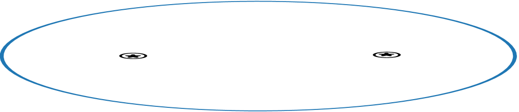
Before predicted
splitting ($t=9$)

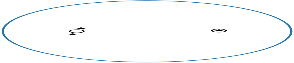
After predicted
splitting ($t=10$)

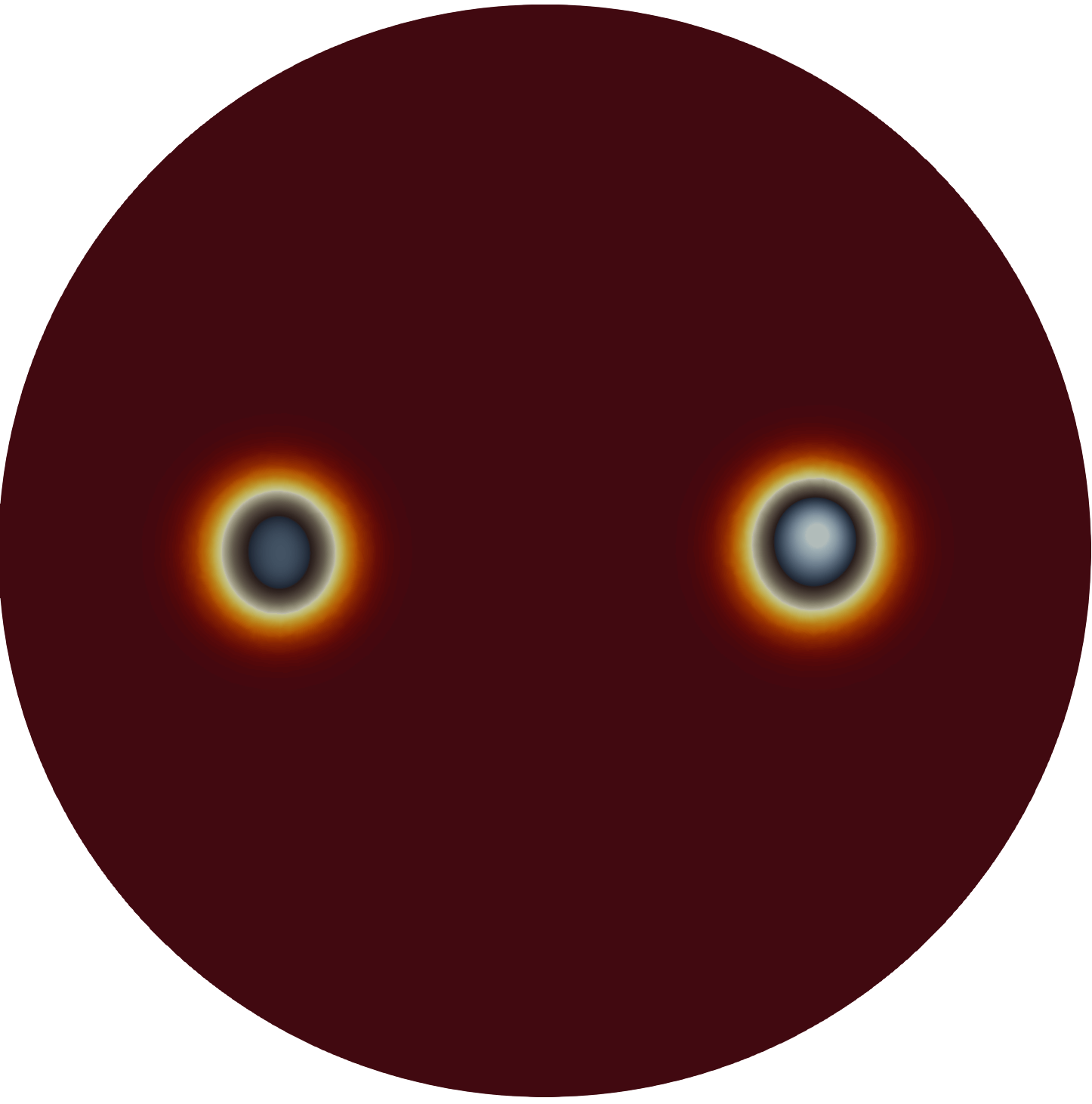
$v$ at $t=10$
 

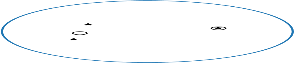
Before actual
splitting ($t=40$)

After actual
splitting ($t=41$)

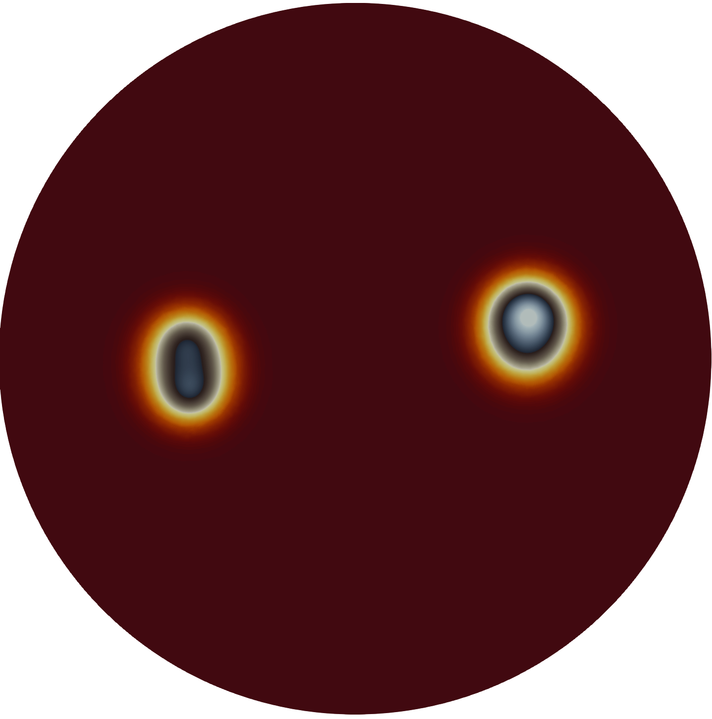
$v$ at $t=41$
 

Figure 29: Left and middle panels: The spot locations obtained from PDE simulation of (5.1) are represented by the black circles. The star markers represent the spot locations from the DAE simulation of (5.23) and (5.21). Right panel: contour plot of $v$ at the indicated time, as computed numerically from the PDE. Parameters are $\varepsilon=0.03$, $a_{0}=19$, $a_{1}=5$, with the concentration point for the feed rate evolving dynamically by (5.11).

5.2.3 A loop of spot replication and spot annihilation

In this subsection we show a PDE simulation of (5.1) that involves a repeating loop of spot replication and annihilation. We choose $\varepsilon=0.03$ and consider a feed rate with $a_{0}=19$ and $a_{1}=5$, where the concentration point $\boldsymbol{\xi}$ of the feed evolves slowly in time according to (5.11). We consider an initial two-spot quasi-equilibrium pattern where the pinned spot is initially at $\boldsymbol{\xi}(0)=(0.5,0)^{T}$ and with an additional unpinned spot initially centered at $(-0.5,0)^{T}$. The PDE simulation results are shown in the right panels of Figs. 29–34 at the indicated times. In the PDE results, we observe that when $t\approx 41$ the unpinned spot splits into two spots. The resulting two spots evolve dynamically and remain separated from the approaching pinned spot. However, as the pinned spot becomes close enough to one of the two unpinned spots, at $t\approx 685$ a competition instability is triggered and one of these spots is annihilated, leaving a pattern with only one spot and the pinned spot. Later at $t\approx 720$, the unpinned spot splits again, and the spot creation-annihilation loop is repeated. We record three cycles of this loop in Figs. 29– 34.

To model this loop theoretically, we introduce an algorithim that combines the DAE dynamics (5.23) and (5.21) with our linear stability theory in §5.2.2 of quasi-equilibrium patterns. Since the DAE system is valid only when there is $\mathcal{O}(1)$ time-scale instability of the quasi-equilibrium pattern, we need to augment the DAE solver with a numerical detection strategy for the initiation of spot-replication or spot-annihilation events, and the subsequent addition or removal of newly created or annihilated spots. At the end of each time step in the DAE solver, we first use (5.35) and the condition $\det\mathcal{M}_{0}=0$ to detect zero-eigenvalue crossings in GCEP. In practice, in our algorithm we identify a zero-eigenvalue crossing if

$$|\det\mathcal{M}_{0}|\leq\mathrm{TOL}\,,\qquad\mbox{where}\quad\mathrm{TOL}\ll 1\,.$$ (5.36)

This zero-eigenvalue crossing corresponds to an inter-spot competition instability, and triggers the annihilation of the spot with the smallest source strength. Once the criterion (5.36) is met, we eliminate that particular spot with $S_{j}=\min\limits_{1\leq i\leq N}S_{i}$ from the DAE system. Next, to detect a peanut-splitting instability, we choose a number $\Sigma_{2}^{\mathrm{eff}}$ that is slightly larger than the peanut splitting threshold $\Sigma_{2}\approx 4.302$ for the unpinned spots. If there is an unpinned spot with $S_{j}>\Sigma_{2}^{\mathrm{eff}}$, the peanut-splitting instability triggers a nonlinear spot creation process that divides the spot into two separate spots. To model this process in our algorithm, we replace this spot at $\mathbf{x}_{j}$, with two new spots located at

$$\mathbf{x}_{new}^{1}=\mathbf{x}_{j}+\delta(v_{2},-v_{1})\,,\qquad\mathbf{x}_{new}^{2}=\mathbf{x}_{j}+\delta(-v_{2},v_{1})\,,$$ (5.37)

where $\delta\ll 1$ and $\mathbf{v}=(v_{1},v_{2})$ is the normalized velocity field ($\,|\mathbf{v}|=1\,$) as computed from the DAE system (5.23) and (5.21). The choice in (5.37) for this two newly created spot locations is motivated from the result in [17], which showed that the direction of spot-splitting is perpendicular to the direction of motion of the spot.

We use this algorithm for augmenting the DAE solver with parameters $\mathrm{TOL}=10^{-4}\,,\enspace\Sigma_{2}^{\mathrm{eff}}=4.4$ and $\delta=0.1$, with results shown in the left and middle panels in Figs. 29– 34. At $t=9$, the algorithm detects a peanut-splitting instability of the spot. The spot is replaced with two spots given in (5.37) (see Fig. 29). Then at $t=583$, the DAE solver detects a zero-eigenvalue crossing based on (5.36). The spot with the minimum source strength is removed from the DAE system. Right after the removal, the DAE solver detects a peanut-splitting instability, and two new spots are created. In conclusion, the DAE solver predicts a spot creation-annihilation event at $t=583$. The PDE simulation confirms a spot annihilation event at $t\approx 684$, and a spot replication event at $t\approx 719$. The DAE solver also predicts the second and third spot creation-annihilation event at $t=1248$ and $t=1952$, respectively. These events are all confirmed by the full PDE simulation (see Fig. 32 and Fig. 33).

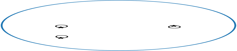
Before predicted killing and splitting ($t=583$)

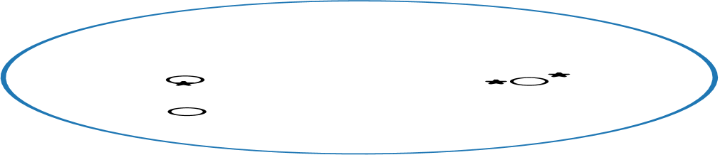
After predicted killing and splitting ($t=584$)

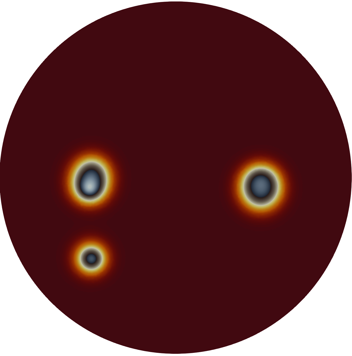
$v$ at $t=584$
 

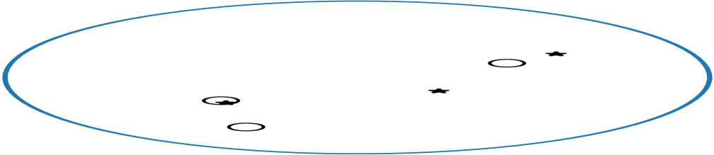
Before actual killing ($t=684$)

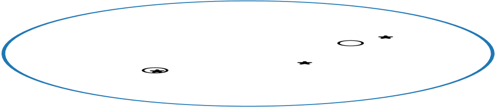
After actual killing ($t=685$)

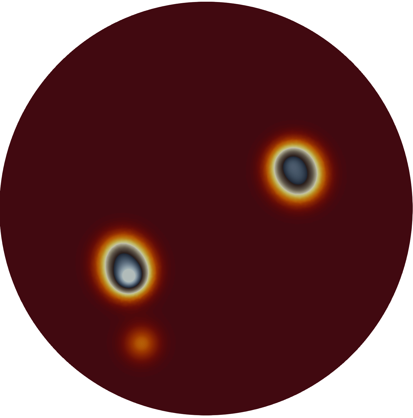
$v$ at $t=684$

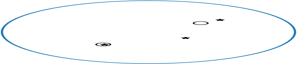
Before actual splitting ($t=719$)

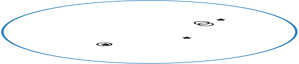
After actual splitting ($t=720$)

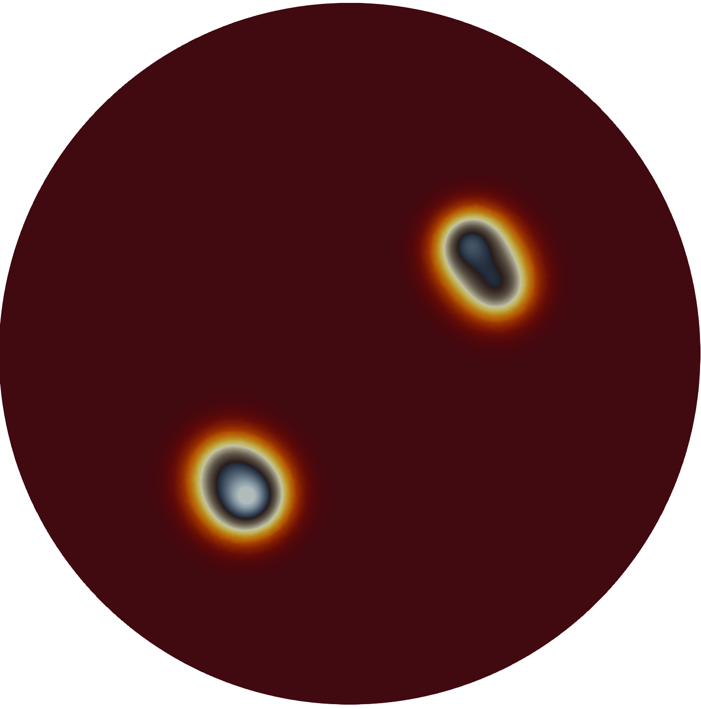
$v$ at $t=720$

Figure 30: Our approximation algorithm detects spot-annihilation and spot-splitting at the same time. On the other hand, the spot-tracking algorithm based on the PDE simulation detects killing and splitting, separately at later time.

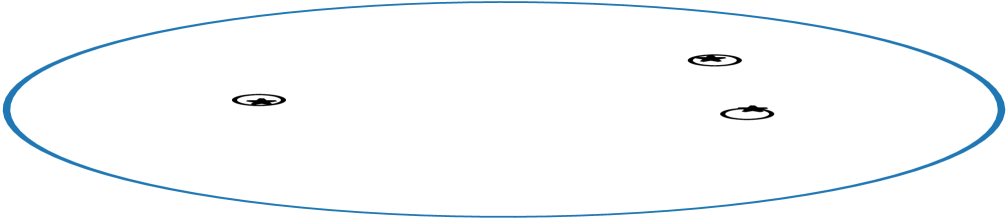
After one cycle ($t=1112$)

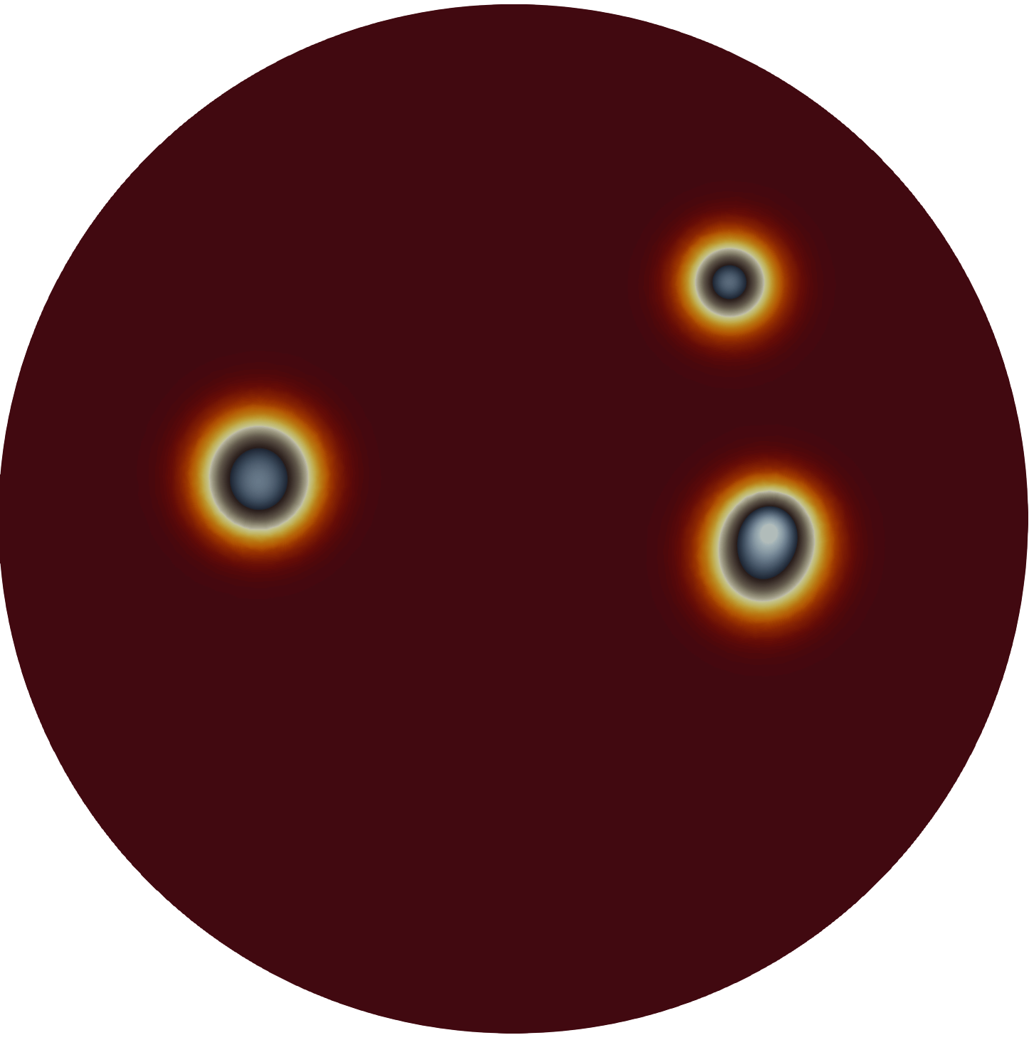
$v$ at $t=1112$

Figure 31: When the pinned-spot finishes a full cycle, the predicted spot location from the DAE and the actual spot location (from the PDE spot-tracking algorithm) have a good agreement. This shows that the spots can catch up with the prediction from the augmented DAE algorithm.

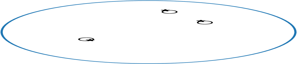
Before predicted killing and splitting ($t=1248$)

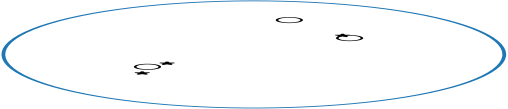
After predicted
killing and splitting
($t=1249$)

$v$ at $t=1249$
 
 

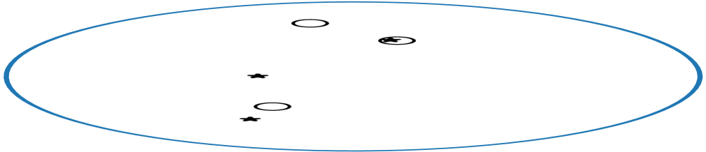
Before actual killing ($t=1350$)

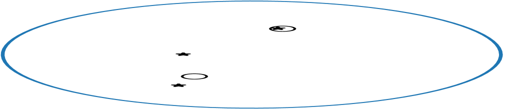
After actual killing ($t=1351$)

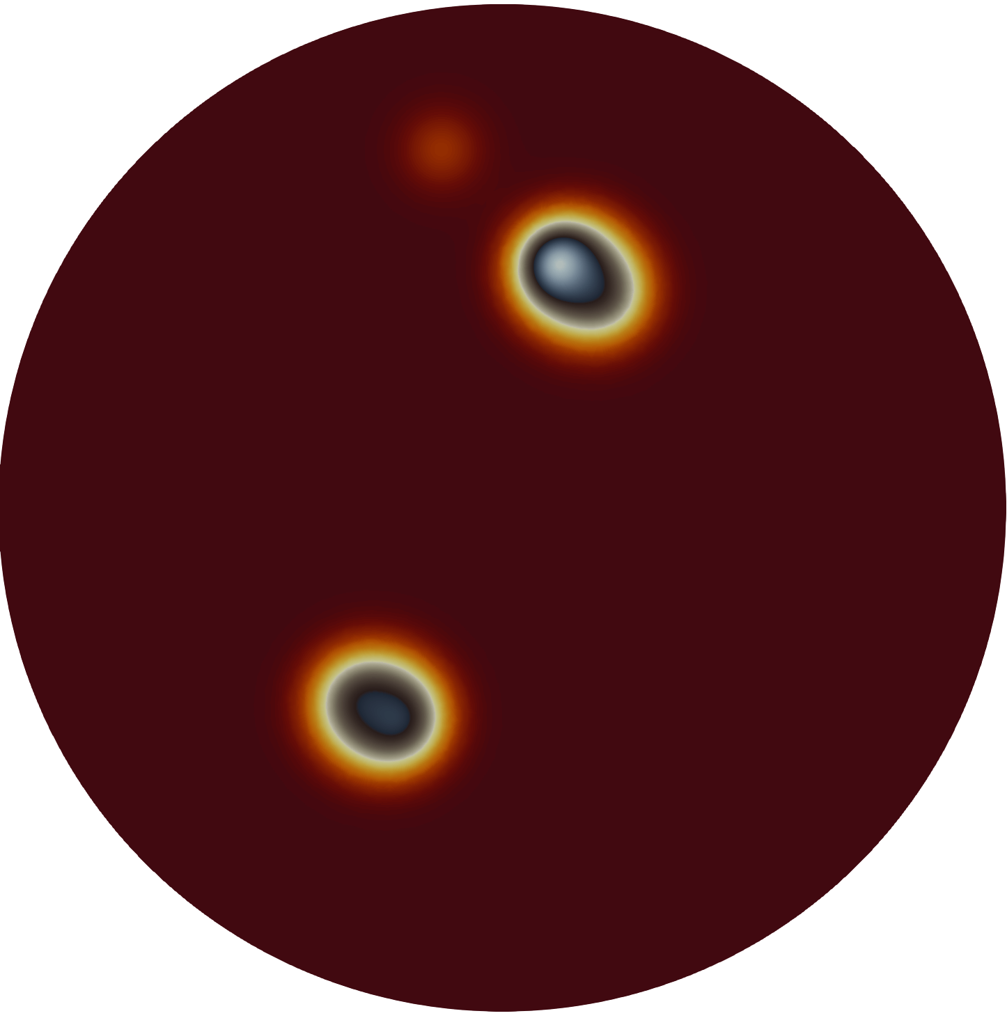
$v$ at $t=1350$

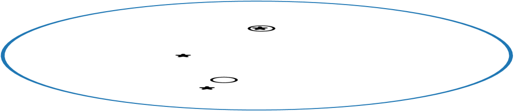
Before actual splitting ($t=1384$)

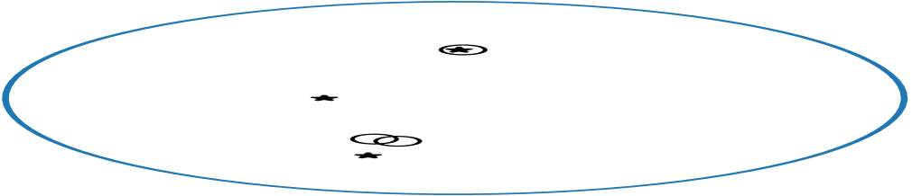
After actual splitting ($t=1385$)

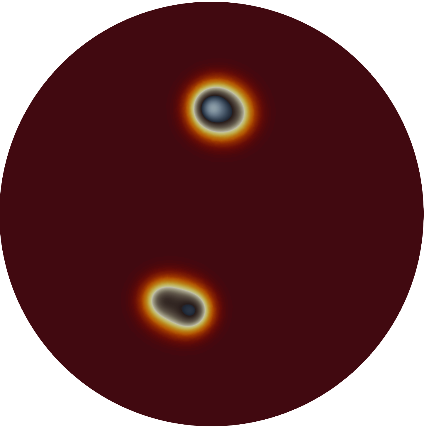
$v$ at $t=1385$

Figure 32: The second spot creation-annihilation event.

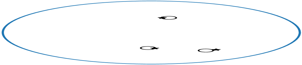
Before predicted killing and splitting ($t=1952$)

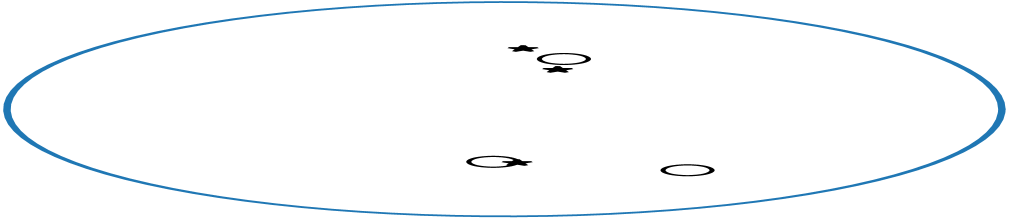
After predicted killing and splitting ($t=1953$)

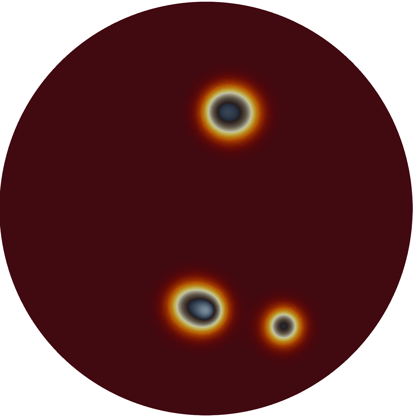
$v$ at $t=1953$
 

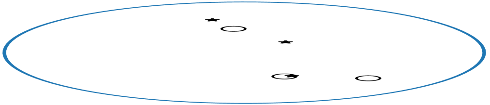
Before actual
killing ($t=2016$)

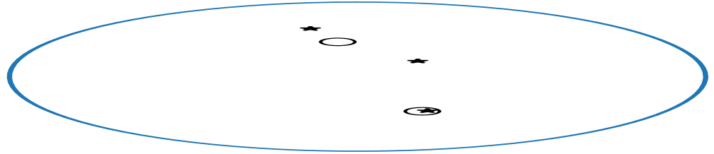
After actual
killing ($t=2017$)

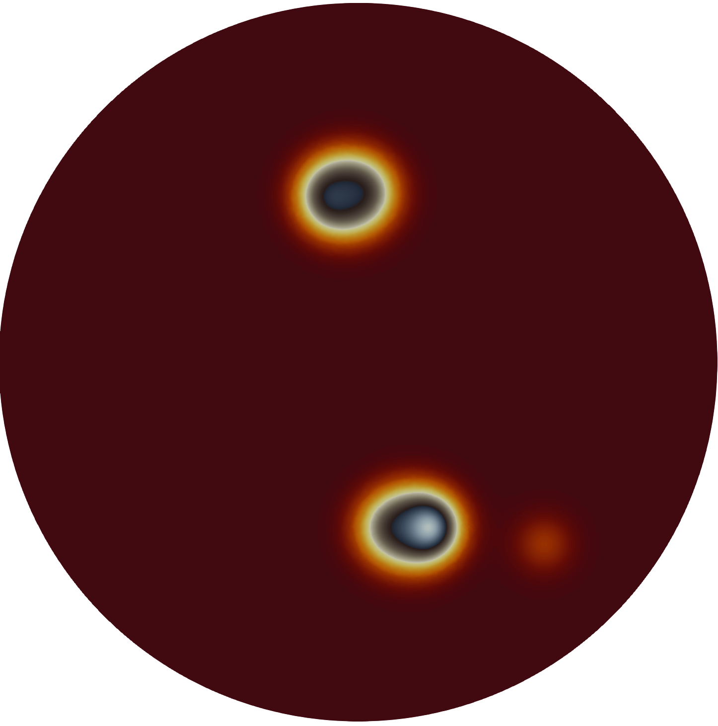
$v$ at $t=2016$
 

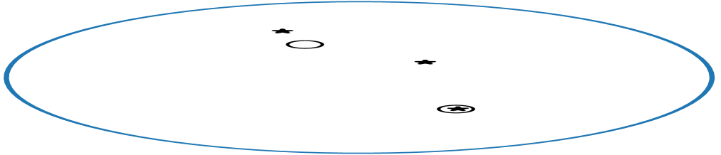
Before actual
splitting ($t=2049$)

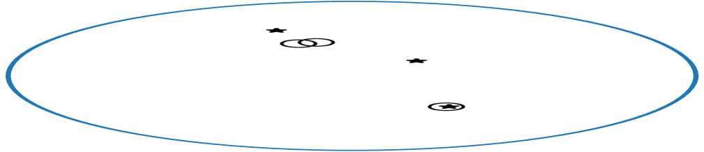
After actual
splitting ($t=2050$)

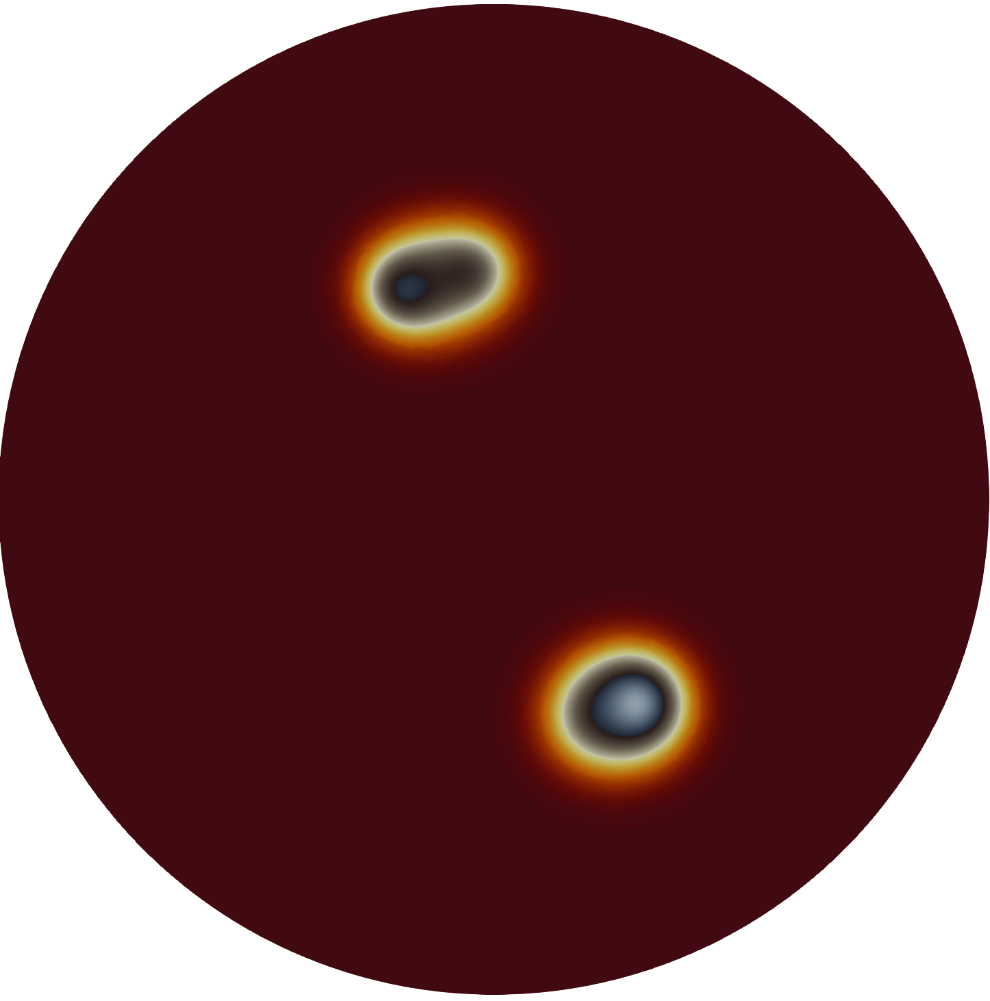
$v$ at $t=2050$
 

Figure 33: The third spot creation-annihilation event

$t=2500$

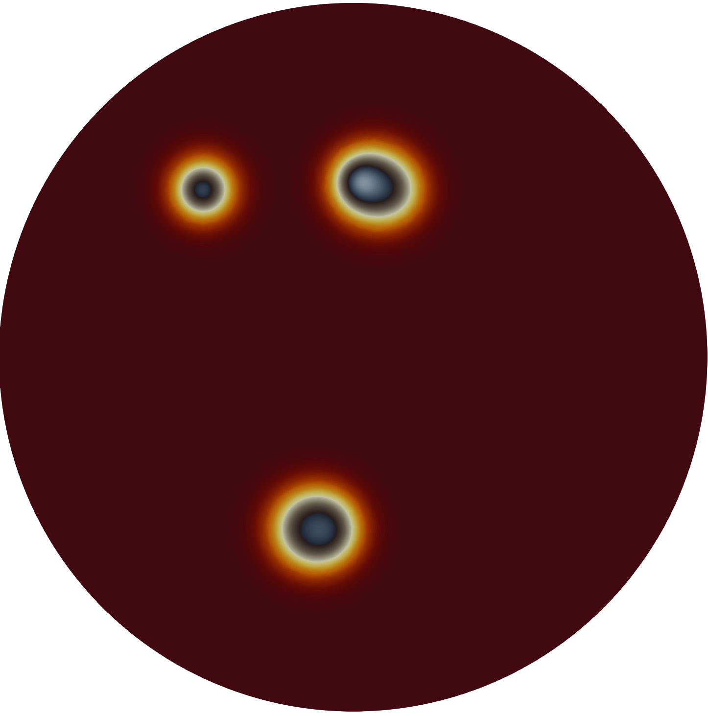
$v$ at $t=2500$

Figure 34: The approximation algorithm provides a reasonably close prediction for the unpinned spot trajectory at $t=2500$ after three spot creation-annihilation events.

6 Discussion

We have developed a hybrid asymptotic-numerical theory to analyze the effect of several types of localized heterogeneities on the existence, linear stability, and slow dynamics of spot patterns for the prototypical two-component Schnakenberg model (1.1) in a bounded 2-D domain. Our analysis has focused on distinct types of localized heterogeneities: a strong localized perturbation of a spatially uniform feed rate and the effect of removing a small hole in the domain, through which the chemical species can leak out. Although our overall approach relies on the theoretical framework first introduced in [17], and later extended in [33] for analyzing the effect of heterogeneities in the Brusselator model, our analysis of localized heterogeneities for the Schnakenberg model has revealed a wide range of novel phenomena such as, saddle-node bifurcations for quasi-equilibrium spot patterns that otherwise would not occur for a homogeneous medium, a new type of spot solution pinned at the concentration point of the feed rate, spot self-replication behavior that generates more than two new spots, and the existence of a creation-annihilation attractor with at most three spots. The hybrid approach presented herein can be readily extended to other well-known RD models such as the Gray-Scott, Gierer-Meinhardt, and Brusselator models.

We conclude by briefly discussing a few problems that warrant further investigation. One interesting direction would be to extend the algorithm, introduced in §5.2.3, to general $N$-spot quasi-equilibrium patterns over much longer time scales. This would involve coupling the ODE-DAE system for slow spot dynamics occuring on long ${\mathcal{O}}(\varepsilon^{-2})$ time scales with sudden “surgeries”, resulting in either spot-creation or spot-annihilation events, that are informed through monitoring linear stability thresholds at each time step as the quasi-equilibrium spot pattern evolves. In particular, in this general setting, it would be interesting to classify whether spot-annihilation events, triggered by a competition instability due to a zero-eigenvalue crossing of the globally coupled eigenvalue problem, can be interpreted more geometrically in terms of crossing through a saddle-node bifurcation point of manifolds of spot quasi-equilibria. Such manifolds depend on the instantaneous spatial configuration of spots, and they evolve slowly in time. For a two-spot pattern in the unit disk, and with a feed rate that is slowly ramped in time, such a fold-point crossing was observed in Fig. 2. In a 1-D setting, spike-annihilation events have been recently interpreted in [4] for the extended Klausmeir RD model as arising from rapid transitions between manifolds of spike quasi-equilibria as the pattern evolves.

Another open problem is to determine whether a creation-annihilation attractor for spot quasi-equilibria, which involves only a few spots, can occur for a time-independent feed rate that has a smooth (not localized) spatial variation. For the 1-D Schnakenberg model, but for a very large number of spikes, such a creation-annihilation attractor has been predicted and observed in [18] through the analysis of a limiting mean-field equation for the spike density.

Finally, it would be interesting to study how variations in the domain geometry or the domain boundary condition influence the slow spot dynamics and the linear stability properties of quasi-equilbrium spot patterns, leading to to new types of spot-pinning behavior. Some work in this direction for the Brusselator model with a Robin boundary condition is given in [33] for the disk. For general domains, the determination of the Neumann Green’s function and the reduced-wave Green’s function would be central to this study. For an elliptical domain of arbitrary eccentricity, spot-pinning behavior can readily be studied using the new analytical result in [12] for the Neumann Green’s function for the ellipse.

Appendix A The Green’s functions for the unit disk

The Neumann Green’s function and its regular part, satisfying (2.9), have explicit formulae for the unit disk (cf. [17]):

$$G(\mathbf{x};\mathbf{z}) =\frac{1}{2\pi}\left(-\log|\mathbf{x}-\mathbf{z}|-\log\left||\mathbf{z}|\mathbf{x}-\frac{1}{|\mathbf{z}|}\mathbf{z}\right|+\frac{1}{2}(|\mathbf{x}|^{2}+|\mathbf{z}|^{2})-\frac{3}{4}\right)\,,$$ (A.1a)

$$R(\mathbf{z};\mathbf{z}) =\frac{1}{2\pi}\left(-\log\left(1-|\mathbf{z}|^{2}\right)+|\mathbf{z}|^{2}-\frac{3}{4}\right)\,.$$ (A.1b)

Their gradients are given by

$$\nabla_{\mathbf{x}}G=-\frac{1}{2\pi}\left(\frac{\left(\mathbf{x}-\mathbf{z}\right)}{|\mathbf{x}-\mathbf{z}|^{2}}+\frac{|\mathbf{z}|^{2}\left(|\mathbf{z}|^{2}\mathbf{x}-\mathbf{z}\right)}{\big{|}|\mathbf{z}|^{2}\mathbf{x}-\mathbf{z}\big{|}}-\mathbf{x}\right)\,,\qquad\nabla_{\mathbf{x}}R=\frac{1}{2\pi}\left(\frac{2-|\mathbf{z}|^{2}}{1-|\mathbf{z}|^{2}}\right)\mathbf{z}\,.$$ (A.2)

For a ring pattern, where $\mathbf{x}_{1},\ldots,\mathbf{x}_{N}$ are equally-spaced on a ring of radius $r_{0}$ concentric within the unit disk as given in (2.39), we have from Proposition 4.3 of [15] that

$$\mathcal{G}\mathbf{e}=\frac{p(r_{0})}{N}\mathbf{e}\,,\qquad p(r_{0})\equiv\frac{1}{2\pi}\left(-N\log(Nr_{0}^{N-1})-N\log(1-r_{0}^{2N})+r_{0}^{2}N^{2}-\frac{3N^{2}}{4}\right)\,.$$ (A.3)

As such, for a ring pattern, there is a symmetric solution to the NAS (2.14) given by $S_{j}=S_{c}={p_{a}/N}$ for $j=1,\ldots,N$, where $p_{a}$ is defined in (2.7). Then, upon defining $\nabla_{\mathbf{x}}R_{j,j}\equiv\nabla_{\mathbf{x}}R(\mathbf{x};\mathbf{x}_{j})|_{\mathbf{x}=\mathbf{x}_{j}}$, and $\nabla_{\mathbf{x}}G_{j,i}\equiv\nabla_{\mathbf{x}}G(\mathbf{x};\mathbf{x}_{i})|_{\mathbf{x}=\mathbf{x}_{j}}$, we then use the reciprocity property of the Green’s function to calculate $\boldsymbol{\beta}_{j}$ in (2.12) as

$$\boldsymbol{\beta}_{j}=2\pi S_{c}\left(\nabla_{\mathbf{x}}R_{j,j}+\sum\limits_{i\neq j}^{N}\nabla_{\mathbf{x}}G_{j,i}\right)=2\pi S_{c}\left(\frac{p^{\prime}(r_{0})}{2N}\right)\mathbf{e}_{\theta_{j}}=S_{c}\left(-\frac{N-1}{2r_{0}}+\frac{Nr_{0}^{2N-1}}{1-r_{0}^{2N}}+Nr_{0}\right)\mathbf{e}_{\theta_{j}}\,,$$ (A.4)

where $\mathbf{e}_{\theta_{j}}\equiv(\cos\theta_{j},\sin\theta_{j})^{T}$ and $\theta_{j}={2\pi(j-1)/N}$. By substituting (A.4) in (2.18), and using $\mathbf{x}_{j}=r_{0}(\sigma)\mathbf{e}_{\theta_{j}}$, we obtain the scalar ODE (2.40) for the ring radius $r_{0}$.

For the unit disk, and for $\lambda\neq 0$, the eigenvalue-dependent Green’s function $G_{\lambda}(\mathbf{x};\mathbf{x}_{0})$, as defined by (2.27), can be expressed as an infinite series as (cf. Appendix A.1 of [7])

$$G_{\lambda}(\mathbf{x};\mathbf{x}_{0})=\frac{1}{2\pi}\left[K_{0}(\theta_{\lambda}|\mathbf{x}-\mathbf{x}_{0}|)-\frac{K_{0}^{\prime}(\theta_{\lambda})}{I_{0}^{\prime}(\theta_{\lambda})}I_{0}(\theta_{\lambda}r)I_{0}(\theta_{\lambda}r_{0})\right]-\frac{1}{\pi}\sum\limits_{n=1}^{\infty}\cos\left[n(\psi-\psi_{0})\right]\frac{K_{n}^{\prime}(\theta_{\lambda})}{I_{n}^{\prime}(\theta_{\lambda})}I_{n}(\theta_{\lambda}r)I_{n}(\theta_{\lambda}r_{0})\,.$$ (A.5a)

Here $$\mathbf{x}=r\,(\cos(\psi),\sin(\psi))\,,\,\mathbf{x}_{0}=r_{0}\,(\cos(\psi_{0}),\sin(\psi_{0})) I_{n} K_{n} n^{\text{th}} \theta_{\lambda} \theta_{\lambda}\equiv\sqrt{\tau\lambda/D} \mathcal{G}_{\lambda}$$, and are the order modified Bessel functions of the first and second kind, respectively, and is the principal branch of . The regular part of is

$$R_{\lambda}(\mathbf{x}_{0};\mathbf{x}_{0})=\frac{1}{2\pi}\left[\log 2-\gamma_{e}-\frac{\log(D/\tau)}{2}-\frac{\log\lambda}{2}-\frac{K_{0}^{\prime}(\theta_{\lambda})}{I_{0}^{\prime}(\theta_{\lambda})}I_{0}^{2}(\theta_{\lambda}r_{0})\right]-\frac{1}{\pi}\sum\limits_{n=1}^{\infty}\frac{K_{n}^{\prime}(\theta_{\lambda})}{I_{n}^{\prime}(\theta_{\lambda})}I_{n}^{2}(\theta_{\lambda}r_{0})\,,$$ (A.5b)

where $\gamma_{e}\approx 0.5772$ is the Euler’s constant.

Appendix B Spectrum of circulant matrices

$\mathcal{A}\in\mathbb{R}^{N\times N}$ is a circulant matrix if every row is obtained by right shifting the previous row by one unit. Therefore, $\mathcal{A}$ can be uniquely determined by it first row, denoted as $\mathbf{a}=(a_{1},\ldots,a_{N})$, while the second row of $\mathcal{A}$ is $(a_{N},a_{1},\ldots,a_{N-1})$. Suppose $\mathcal{A}$ is symmetric and circulant. Then, the eigenvalues of $\mathcal{A}$ are

$$\lambda_{1}=\sum\limits_{k=1}^{N}a_{k}\,,\qquad\lambda_{j}=\sum\limits_{k=0}^{N-1}\cos\left[\frac{2\pi(j-1)k}{N}\right]\,a_{k+1}\,,\quad j=2,\ldots,N\,.$$ (B.1a)

The corresponding eigenvectors are $$\mathbf{q}_{1}=\mathbf{e}=(1,\ldots,1)^{T}\in\mathbb{R}^{N}$$ and

$$,\begin{split}\mathbf{q}_{j}&=\left(1\,,\cos\left(\frac{2\pi(j-1)}{N}\right)\,,\ldots\,,\cos\left(\frac{2\pi(j-1)(N-1)}{N}\right)\right)^{T}\,,\\[5.0pt] \mathbf{q}_{N+2-j}&=\left(0\,,\sin\left(\frac{2\pi(j-1)}{N}\right)\,,\ldots\,,\sin\left(\frac{2\pi(j-1)(N-1)}{N}\right)\right)^{T}\,,\end{split}$$ (B.1b)

for $$j=2,\dots,\mathrm{ceil}(N/2) \mathrm{ceil}(s) s N \lambda_{N/2+1} \mathbf{q}_{N/2+1}=(1,-1,\ldots,1,-1)^{T}$$, where denotes the smallest integer that is not less than . Furthermore, when is even, we have an additional simple eigenvalue with eigenvector .

References

- [1] M. Alnæs, J. Blechta, J. Hake, A. Johansson, B. Kehlet, A. Logg, C. Richardson, J. Ring, M. E. Rognes, and G. N. Wells. The fenics project version 1.5. Archive of Numerical Software, 3(100), 2015.
- [2] D. Avitabile, V. F. Bren͂a, and M. J. Ward. Spot dynamics in a reaction-diffusion model of plant root hair initiation. SIAM J. Appl. Math., 78(1):291–319, 2018.
- [3] R. Bastiaansen, M. Chirilus-Bruckner, and A. Doelman. Pulse solutions for an extended Klausmeier model with spatially varying coefficients. SIAM J. Appl. Dyn. Sys., 19(1):1–57, 2020.
- [4] R. Bastiaansen and A. Doelman. The dynamics of disappearing pulses in a singularly perturbed reaction-diffusion system with parameters that vary in space and time. Physica D, 388:45–72, 2019.
- [5] V. F. Bren͂a, A. Champneys, C. Grierson, and M. J. Ward. Mathematical modeling of plant root hair initiation: Dynamics of localized patches. SIAM J. Appl. Dyn. Sys., 13(1):210–248, 2014.
- [6] C. N. Chen, S. I. Ei, and S. Tzeng. Heterogeneity-induced effects for pulse dynamics in Fitzhugh-Nagumo-type systems. Physica D, 382-383(1):22–32, 2018.
- [7] W. Chen and M. J. Ward. The stability and dynamics of localized spot patterns in the two-dimensional Gray-Scott model. SIAM J. Appl. Dyn. Sys., 10(2):582–666, 2011.
- [8] H. Dankowicz and F. Schilder. Recipes for continuation, volume 11 of Computational Science & Engineering. Society for Industrial and Applied Mathematics (SIAM), Philadelphia, PA, 2013.
- [9] P. Davies, P. Blanchedeau, E. Dulos, and P. De Kepper. Dividing blobs, chemical flowers, and patterned islands in a reaction- diffusion system. J. Phys. Chem. A, 102(43):8236–8244, 1998.
- [10] A. Doelman, P. van Heijster, and J. Shen. Pulse dynamics in reaction-diffusion systems with strong spatially localized impurities. Phil. Trans. Roy. Soc. A., 376:20170183, 2018.
- [11] H. Ikeda and S. I. Ei. Front dynamics in heterogeneous diffusive media. Physica D., 239:1637–1649, 2010.
- [12] S. Iyaniwura, T. Wong, C. B. MacDonald, and M. J. Ward. Optimization of the mean first passage time in near-disk and elliptical domains in 2-D with small absorbing traps. SIAM Review, 2020, submitted.
- [13] L. T. J.C. Tzou. Spot patterns of the Schnakenberg reaction-diffusion system on a curved torus. Preprint, 2019.
- [14] E. Knobloch. Spatial localization in dissipative systems. Annu. Rev. Cond. Mat. Phys., 6:325–359, 2015.
- [15] T. Kolokolnikov, M. S. Titcombe, and M. J. Ward. Optimizing the fundamental Neumann eigenvalue for the Laplacian in a domain with small traps. European J. of Appl. Math., 16(2):161–200, 2005.
- [16] T. Kolokolnikov, M. Ward, J. Tzou, and J. Wei. Stabilizing a homoclinic stripe. Phil. Trans. Roy. Soc. A., 376(2135):20180110, 2018.
- [17] T. Kolokolnikov, M. J. Ward, and J. Wei. Spot self-replication and dynamics for the Schnakenburg model in a two-dimensional domain. J. Nonlinear Science, 19(1):1–56, 2009.
- [18] T. Kolokolnikov and J. Wei. Pattern formation in a reaction-diffusion system with space-dependent feed rate. SIAM Review, 60(3):626–645, 2018.
- [19] T. Kolokolnikov and J. Wei. Hexagonal spike clusters for some pde’s in 2-d. DCDS-B, 25(10):4057–4070, 2020.
- [20] T. Kolokolnikov and S. Xie. Spike density distribution for the Gierer-Meinhardt model with precursor. Physica D, 31:132247, 2019.
- [21] T. Kolokolniov, F. Paquin-Lefebvre, and M. J. Ward. Stable asymmetric spike equilibria for the Gierer-Meinhardt model with a precursor field. IMA J. of Appl. Math, 2020, (to appear).
- [22] A. L. Krause, V. Klika, T. E. Woolley, and E. A. Gaffney. Heterogeneity induces spatiotemporal oscillations in reaction-diffusion systems. Phys. Rev. E, 97(5):052206, 2018.
- [23] A. L. Krause, V. Klika, T. E. Woolley, and E. A. Gaffney. From one pattern into another: Analysis of Turing patterns in heterogeneous domains via WKBJ. J. Roy. Soc. Interface, 17:20190621, 2020.
- [24] V. Kurella, J. C. Tzou, D. Coombs, and M. J. Ward. Asymptotic analysis of first passage time problems inspired by ecology. Bull. Math. Biol., 77(1), 2015.
- [25] K.-J. Lee, W. D. McCormick, J. E. Pearson, and H. L. Swinney. Experimental observation of self-replicating spots in a reaction–diffusion system. Nature, 369(6477):215–218, 1994.
- [26] K. J. Lee and H. L. Swinney. Lamellar structures and self-replicating spots in a reaction-diffusion system. Phys. Rev. E, 51(3):1899, 1995.
- [27] K. Nishi, Y. Nishiura, and T. Teramoto. Dynamics of two interfaces in a hybrid system with jump-type heterogeneity. Japan J. Indust. Appl. Math., 30:351–395, 2013.
- [28] Y. Nishiura, T. Teramoto, and X. Yuan. Heterogeneity-induced spot dynamics for a three-component reaction-diffusion system. Comm. Pure and Appl. Anal., 11(1):307–338, 2012.
- [29] K. Page, P. K. Maini, and N. A. M. Monk. Pattern formation in spatially heterogeneous turing reaction-diffusion models. Physica D, 181(1-2):80–101, 2003.
- [30] K. Page, P. K. Maini, and N. A. M. Monk. Complex pattern formation in reaction-diffusion systems with spatially varying parameters. Physica D, 202(1-2):95–115, 2005.
- [31] I. Rozada, S. J. Ruuth, and M. Ward. The stability of localized spot patterns for the Brusselator on the sphere. SIAM J. Appl. Dyn. Sys., 13(1):564–627, 2014.
- [32] P. H. Trinh and M. J. Ward. The dynamics of localized spot patterns for reaction-diffusion systems on the sphere. Nonlinearity, 29(3):766, 2016.
- [33] J. C. Tzou and M. J. Ward. The stability and slow dynamics of spot patterns in the 2D Brusselator model: The effect of open systems and heterogeneities. Physica D, 373:13–37, 2018.
- [34] P. van Heijster, C. N. Chen, Y. Nishiura, and T. Teramoto. Pinned solutions in a heterogeneous three-component FitzHugh-Nagumo model. Journal of Dynamics and Differential Equations, 31(1):153–203, 2019.
- [35] P. van Heijster, A. Doelman, T. J. Kaper, Y. Nishiura, and K. I. Ueda. Pinned fronts in heterogeneous media of jump type. Nonlinearity, 24(1):127–157, 2010.
- [36] V. K. Vanag and I. R. Epstein. Localized patterns in reaction-diffusion systems. Chaos, 17(3):037110, 2007.
- [37] M. J. Ward, W. D. Henshaw, and J. B. Keller. Summing logarithmic expansions for singularly perturbed eigenvalue problems. SIAM J. Appl. Math., 53(3):799–828, 1993.
- [38] M. J. Ward and J. B. Keller. Strong localized perturbations of eigenvalue problems. SIAM J. Appl. Math., 53(3):770–798, 1993.
- [39] M. J. Ward, D. McInerney, H. P., G. D., and P. Maini. The dynamics and pinning of a spike for a reaction-diffusion model. SIAM J. Appl. Math., 62(4):1297–1328, 2002.
- [40] J. Wei and M. Winter. Asymmetric spotty patterns for the Gray–Scott model in . Studies in Appl. Math., 110(1):63–102, 2003.
- [41] J. Wei and M. Winter. Existence and stability of multiple-spot solutions for the Gray–Scott model in . Physica D: Nonlinear Phenomena, 176(3-4):147–180, 2003.
- [42] J. Wei and M. Winter. Stationary multiple spots for reaction–diffusion systems. Journal of mathematical biology, 57(1):53–89, 2008.
- [43] J. Wei and M. Winter. On the Gierer-Meinhardt system with precursors. DCDS-A, 25(1):363–398, 2009.
- [44] J. Wei and M. Winter. Spikes for the Gierer-Meinhardt system with discontinuous diffusion coefficients. J. Nonlinear Sci., 12(3):301–339, 2009.
- [45] J. Wei and M. Winter. Stable spike clusters for the one-dimensional Gierer-Meinhardt system. European J. of Appl. Math., 28(4):576–635, 2017.
- [46] T. Wong and M. J. Ward. Weakly nonlinear analysis of peanut-shaped deformations for localized spots of singularly perturbed reaction-diffusion systems. SIAM J. Appl. Dyn. Sys., 2020, to appear.
- [47] S. Xie and T. Kolokolnikov. Moving and jumping spot in a two-dimensional reaction–diffusion model. Nonlinearity, 30(4):1536, 2017.
- [48] X. Yuan, T. Teramoto, and Y. Nishiura. Heterogeneity-induced defect bifurcation and pulse dynamics for a three-component reaction-diffusion system. Phys. Rev. E., 75(036220), 2007.