Network model for higher-order topological phases

Abstract

We introduce a two-dimensional network model that realizes a higher-order topological phase (HOTP). We find that in the HOTP the bulk and boundaries of the system are gapped, and a total of 16 corner states are protected by the combination of a four-fold rotation, a phase-rotation, and a particle-hole symmetry. In addition, the model exhibits a strong topological phase at a point of maximal coupling. This behavior is in opposition to conventional network models, which are gapless at this point. By introducing the appropriate topological invariants, we show how a point group symmetry can protect a topological phase in a network. Our work provides the basis for the realization of HOTP in alternative experimental platforms implementing the network model.

I Introduction

Topological phases of matter are known to support boundary modes which are protected by bulk topological invariants through the so-called bulk-boundary correspondence. The topological protection is typically associated with fundamental symmetries (time-reversal, particle-hole, and chiral symmetry) which have led to the tenfold classification of (gapped) topological states Schnyder et al. (2008); Ryu et al. (2010); Chiu et al. (2016). By further including discrete spatial symmetries, new phases such as topological crystalline phases Mong et al. (2010); Fu (2011); Slager et al. (2013); Ando and Fu (2015); Chiu et al. (2013) and, very recently, higher-order topological phases (HOTPs) have been identified Benalcazar et al. (2017a, b); Langbehn et al. (2017); Song et al. (2017); Schindler et al. (2018a, b); Geier et al. (2018); Khalaf (2018); Trifunovic and Brouwer (2019); Wang et al. (2018a); van Miert and Ortix (2018); You et al. (2018); Călugăru et al. (2019); Araki et al. (2019); Kudo et al. (2019); Tiwari et al. (2020); Ezawa (2018a, b); Hsu et al. (2018); Wang et al. (2018b); Yan et al. (2018); Ghorashi et al. (2020a, b, 2019).

A prototypical HOTP is the Benalcazar-Bernevig-Hughes (BBH) model Benalcazar et al. (2017a), where fundamental and point group symmetries protect zero-energy corner states in an otherwise gapped, two-dimensional (2D) system . HOTPs have already been realized in various platforms ranging from photonic, phononic, and electronic systems to microwave and topoelectric circuits Serra-Garcia et al. (2018); Peterson et al. (2018); Imhof et al. (2018); Serra-Garcia et al. (2019); Zhang et al. (2019); Kempkes et al. (2019); Yue et al. (2019); Mittal et al. (2019); Xue et al. (2019); Ni et al. (2019); El Hassan et al. (2019).

Ever since the discovery of the quantum Hall effect, a main focus of research has been to study the robustness of topological states against disorder, and the associated localization-delocalization transitions that destroy a topological phase Evers and Mirlin (2008). Among other approaches, a powerful tool in this study has been the network model description of topological phases Evers and Mirlin (2008); Chalker and Coddington (1988); Kramer et al. (2005), first introduced by Chalker and Coddington (CC) in the context of the quantum Hall effect Chalker and Coddington (1988). The network model idea has subsequently been adapted to a variety of different topological systems, including the quantum spin-Hall effect, weak topological insulators, Floquet systems, as well as different types of topological superconductors Kagalovsky et al. (1999); Chalker et al. (2001); Beamond et al. (2002); Obuse et al. (2007, 2014); Fulga et al. (2012a); Pasek and Chong (2014); De Beule et al. (2020). However, despite their versatility, no network models for point group symmetry-protected topological phases have been introduced to date. This includes HOTPs, which are very recent additions to the list of topological systems, but also conventional topological crystalline phases, which are by now a decade old Mong et al. (2010); Fu (2011).

Here, we construct a network model for a HOTP protected by particle-hole and by fourfold rotation ($C_{4}$) symmetry, which hosts mid gap corner modes. Unlike the $C_{4}$-symmetric HOTPs in static systems, which have 4 corner states Benalcazar et al. (2017a, b), or their periodically driven counterparts, where this number can go up to 8 Rodriguez-Vega et al. (2019); Bomantara et al. (2019); Huang and Liu (2020), our network model shows up to 16 corner modes, due to an additional, phase-rotation symmetry Delplace et al. (2017). Upon varying system parameters, we find that the trivial phase and the HOTP are separated by an intermediate, strong topological phase (STP), which surprisingly is present even at the point of maximal mode mixing, i.e., when the reflection and transmission probabilities are equal. This behavior is in sharp contrast to the conventional Chalker-Coddington model and its generalizations Kagalovsky et al. (1999); Chalker et al. (2001); Beamond et al. (2002); Obuse et al. (2007, 2014); Fulga et al. (2012a); Pasek and Chong (2014), all of which are gapless at this point.

The rest of this work is organized as follows. In Sec. II, we describe the construction of the network model and examine its symmetries. In Sec. III we analyze several simple limits of the network model, which realize a HOTP, a trivial, and a STP. A detailed study of the phase diagram is performed in Sec. IV, and the topological invariants of the system are calculated in Sec. V. We study the effect of disorder in Sec. VI and comment on experimental realizations of network models in Sec. VII. We conclude in Sec. VIII.

II Network model

The CC network model is a 2D square lattice consisting of directed links and nodes. It models a quantum Hall device where the links correspond to chiral edge states which propagate along equipotential lines, and the nodes correspond to saddle points in the potential where scattering between the edge states takes place Chalker and Coddington (1988). Each node of the CC network model connects two incoming to two outgoing states, being described by a $2\times 2$ unitary scattering matrix

$$S=\begin{pmatrix}\mathfrak{r}&\mathfrak{t}^{\prime}\\ \mathfrak{t}&\mathfrak{r}^{\prime}\end{pmatrix},$$ (1)

where $\mathfrak{r},\mathfrak{r}^{\prime}$ and $\mathfrak{t},\mathfrak{t}^{\prime}$ are (generally complex valued) reflection and transmission amplitudes, respectively. By imposing constraints on the form of $S$ while keeping the lattice structure intact, one can include the effect of fundamental symmetries on the network model. The CC network model can thus be extended to describe topological phases in a variety of Altland-Zirnbauer (AZ) classes (Altland and Zirnbauer, 1997; Evers and Mirlin, 2008; Kagalovsky et al., 1999; Chalker et al., 2001; Fulga et al., 2012a; Obuse et al., 2014; Beamond et al., 2002; Obuse et al., 2007; Pasek and Chong, 2014; Son and Raghu, ).

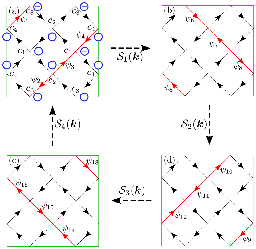
Figure 1: Unit cell of the network model. The arrows represent chiral Majorana modes with wavefunctions $\psi_{i}$. Their intersections represent scattering nodes. The scattering amplitudes at the different nodes are parametrized by the angles $\theta_{i}$, with $c_{i}\equiv\cos\theta_{i}$. The symbol $\ominus$ denotes the fact that the scattered wave acquires a $\pi$-phase shift with respect to the incoming amplitude [see Eq. (2)]. We introduce the notation $\Psi_{i}=(\psi_{4i-3},\psi_{4i-2},\psi_{4i-1},\psi_{4i})^{T}$ with $\Psi_{i}=\Psi_{i+4}$, $i=1,2,3,4$, see the red arrows. The wavefunctions are related to each other via $\Psi_{i+1}=\mathcal{S}_{i}(\bm{k})\Psi_{i}$ [see Eqs. (5)–(9)].

To construct a network model for a HOTP, we need both fundamental as well as point group symmetries, meaning that both the form of $S$ as well as the lattice structure of the network model should be modified. We choose a unit cell composed of 8 nodes and 16 links, four times larger than that of the original CC model, see Fig. 1. We impose particle-hole symmetry, such that the model belongs to the AZ class D. The directed links of the network correspond to chiral Majorana modes and the scattering matrices are real, $S^{\phantom{{\dagger}}}_{i}=S_{i}^{*}$, with $i$ labeling different nodes. This allows to parametrize them in terms of an angle $\theta_{i}$ and a relative sign $\pm$ as

$$S_{i}=\begin{pmatrix}\cos{\theta_{i}}&\mp\sin{\theta_{i}}\\ \sin{\theta_{i}}&\pm\cos{\theta_{i}}\end{pmatrix}.$$ (2)

In Fig. 1, we have indicated the minus signs connecting an incoming and an outgoing amplitude per node by the symbol $\ominus$. In the following, we will examine the behavior of the network model as a function of four different angles $\theta_{1},\ldots,\theta_{4}$ in the unit cell, see Fig. 1 for the convention. As we will show below, imposing a $C_{4}$ symmetry implies setting $\theta_{1}=\theta_{2}$ and $\theta_{3}=\theta_{4}$.

A network model consisting of $N$ links can be described using the wavefunction $\Phi=(\psi_{1},\psi_{2},\ldots,\psi_{N})^{T}$, where $\psi_{j}$ denotes the amplitude on link $j$ of the network. As waves propagate through the network, they are scattered into each other at the nodes, a process modeled as a discrete-time evolution Ho and Chalker (1996); Janssen et al. (1999)

$$\psi_{j}(t+1)=\sum_{k}{\cal S}_{jk}\psi_{k}(t),$$ (3)

with $t\in\mathbb{Z}$ the discrete time unit and ${\cal S}$ a unitary matrix (also known as the Ho-Chalker operator Ho and Chalker (1996)) containing the transmission and reflection amplitudes of the scattering nodes. A stationary state of the network model obeys the relation

$${\cal S}\Phi=e^{-i\varepsilon}\Phi.$$ (4)

The above equation is reminiscent of the Floquet treatment of periodically driven systems, where now the role of the Floquet operator is taken by the unitary matrix ${\cal S}$, and its eigenphases $\varepsilon$ play the role of the quasienergies. By solving Eq. (4), we gain access to the spectrum of the network model, enabling us to identify gaps in the spectrum of eigenphases and potential corner modes. Furthermore, by considering an infinite, translationally invariant network model, Eq. (4) provides access to the ”bandstructure” $\varepsilon({\bm{k}})$ of the system with ${\bm{k}}=(k_{x},k_{y})$ the two wavenumbers.

In our network model, the momentum space Ho-Chalker operator in the translationally invariant setting is a $16\times 16$ matrix, due to the fact that there are 16 links per unit cell. Using the labeling convention of Fig. 1, it reads

$$\mathcal{S}(\bm{k})=\begin{pmatrix}0&0&0&\mathcal{S}_{4}(\bm{k})\\ \mathcal{S}_{1}(\bm{k})&0&0&0\\ 0&\mathcal{S}_{2}(\bm{k})&0&0\\ 0&0&\mathcal{S}_{3}(\bm{k})&0\end{pmatrix},$$ (5)

where the blocks are given by

$$\mathcal{S}_{1}(\bm{k})=\begin{pmatrix}e^{-ik_{y}}\sin\theta_{3}&\cos\theta_{3}&0&0\\ \cos\theta_{3}&-e^{ik_{y}}\sin\theta_{3}&0&0\\ 0&0&\cos\theta_{1}&\sin\theta_{1}\\ 0&0&\sin\theta_{1}&-\cos\theta_{1}\end{pmatrix},$$ (6)

$$\mathcal{S}_{2}(\bm{k})=\begin{pmatrix}e^{ik_{x}}\sin\theta_{4}&0&0&\cos\theta_{4}\\ 0&\cos\theta_{2}&\sin\theta_{2}&0\\ 0&\sin\theta_{2}&-\cos\theta_{2}&0\\ \cos\theta_{4}&0&0&-e^{-ik_{x}}\sin\theta_{4}\end{pmatrix},$$ (7)

$$\mathcal{S}_{3}(\bm{k})=\mathcal{S}_{1}(\bm{k})\;[k_{y}\mapsto-k_{y},\theta_{3}\mapsto-\theta_{3},\theta_{1}\mapsto\pi-\theta_{1}],$$ (8)

$$\mathcal{S}_{4}(\bm{k})=\mathcal{S}_{2}(\bm{k})\;[k_{x}\mapsto-k_{x}].$$ (9)

In the translationally invariant system, particle-hole symmetry is expressed as ${\cal S}({\bm{k}})={\cal S}^{*}(-{\bm{k}})$. This is reminiscent of Floquet systems and indicates that for any eigenstate of the network model at eigenphase $\varepsilon$ and momentum ${\bm{k}}$, there exists another eigenstate at $-\varepsilon$ and $-{\bm{k}}$. Further, along the line $\theta_{1}=\theta_{2}$, $\theta_{3}=\theta_{4}$, the Ho-Chalker operator has $C_{4}$ symmetry $\mathcal{R}$ with ${\cal R}{\cal S}(k_{x},k_{y}){\cal R}^{\dagger}={\cal S}(k_{y},-k_{x})$, where

$${\cal R}=\begin{pmatrix}0&0&0&{\cal R}_{4}\\ {\cal R}_{3}&0&0&0\\ 0&{\cal R}_{2}&0&0\\ 0&0&{\cal R}_{1}&0\end{pmatrix},\quad{\cal R}_{i}=K_{i}\begin{pmatrix}1&0&0&0\\ 0&0&0&1\\ 0&0&1&0\\ 0&1&0&0\end{pmatrix};$$ (10)

$K_{i}$ is a $4\times 4$ diagonal matrix whose $i$-th diagonal element is $-1$ while the others are $1$.

Finally, the Ho-Chalker operator ${\cal S}$ also possesses a so-called phase-rotation symmetry (PRS) ${\cal Z}{\cal S}(\bm{k}){\cal Z}^{\dagger}=e^{i\pi/2}{\cal S}(\bm{k})$, with ${\cal Z}=\mathop{\rm diag}(i,-1,-i,1)\otimes\mathbbm{1}_{4}$ the phase-rotation operator Delplace et al. (2017). The latter symmetry implies that for any eigenstate with eigenphase $\varepsilon$ there also exists an eigenstate at $\varepsilon+\pi/2$. As such, the spectrum of the network model repeats four times in $\varepsilon\in[-\pi,\pi)$, allowing to focus on the ”fundamental phase domain” with $\varepsilon\in[-\pi/4,\pi/4)$.

The phase-rotation symmetry arises due to the geometry of the network model, as explained in Ref. Delplace et al. (2017). Specifically, it is due to the fact that it consists of unidirectional modes which are coupled to each other in a cyclic way, as shown in Fig. 1. Thus, it can be thought of as a structural constraint, similar to the more familiar lattice symmetries such as rotation. Unlike rotations, however, the phase rotation symmetry is unique to unitary operators, since in a Hermitian Hamiltonian the energy shift associated to it would be unphysical.

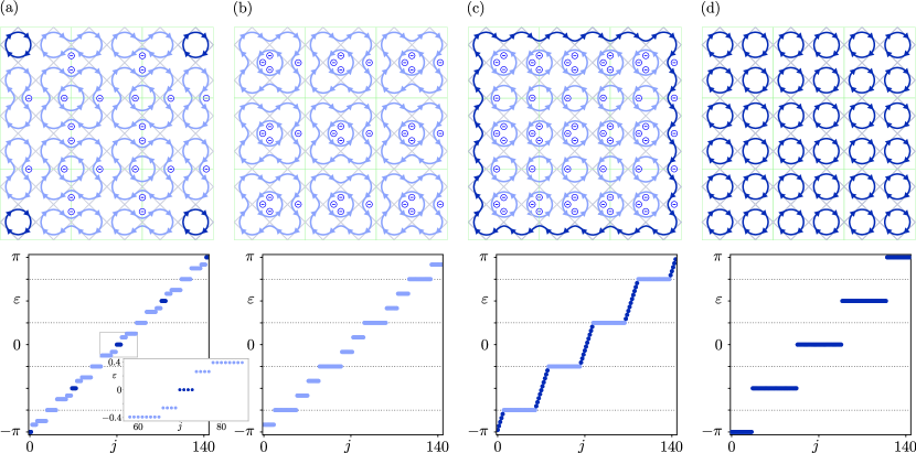
Figure 2: The top panels show the network model, consisting of $3\times 3$ unit cells, in the four decoupled limits: HOTP ($\theta_{1}=\theta_{3}=\pi/2$) in panel (a), trivial ($\theta_{1}=\theta_{3}=0$) in panel (b), STP ($\theta_{1}=0$, $\theta_{3}=\pi/2$) in panel (c), and Majorana flat band ($\theta_{1}=\pi/2$, $\theta_{3}=0$) in panel (d). The bottom panels show the spectra of the Ho-Chalker operators in the same limits. The inset in panel (a) is a closeup of the midgap corner modes. Gapped (gapless) modes and the Majorana loops producing them are shown in light (dark) blue. The horizontal dotted lines mark the boundaries of the fundamental phase domain, which repeats four times due to phase-rotation symmetry. Notice that all gapped Majorana loops contain an odd number of minus signs (denoted by $\ominus$) in a closed loop. See Fig. 1 for the minus sign conventions within a unit cell.

III Decoupled limits

We study the network model by first focusing on the $C_{4}$-symmetric case where the network properties are controlled by the two angles $\theta_{1}(=\theta_{2})$ and $\theta_{3}(=\theta_{4})$, corresponding to the mixing angle at the inner and outer nodes of the unit cell, see Fig. 1. To determine the properties of the edge and corner states, we construct finite-sized network models by imposing open boundary conditions (OBC) in both directions. As shown in Fig. 2, the OBC are obtained by demanding that the Majorana wavefunctions impinging on the boundary are reflected with unit probability, which implies a vanishing of the probability current across the boundary.

First, we investigate the four ‘decoupled limits’ of the network model, obtained when $\theta_{i}$ are either $0$ or $\pi/2$. For these values, the incoming Majorana modes do not get mixed by node scattering but instead turn either clockwise or counterclockwise with unit probability, see Fig. 2. The system then consists of Majorana modes propagating along closed loops that are fully decoupled from each other.

In this limit, we can determine the spectrum of the network model entirely from the structure of these closed loops. For a closed path consisting of $\ell$ links, a Majorana wavefunction comes back to itself after $\ell$ discrete time steps, i.e., after $\ell$ applications of the Ho-Chalker operator of Eq. (3). Note that there are only two options after a full loop. Either the link amplitude picks up a total phase of 0 (periodic) or $\pi$ (antiperiodic), since the Majorana wavefunction is real. The spectrum of the system can thus be determined from the lengths of these loops. All periodic loops of length $\ell$ contribute to the spectrum of the Ho-Chalker operator with the eigenphases $\varepsilon=2\pi k/\ell$, where $k=0,1,\ldots,\ell-1$. As such, they admit a gapless solution with an eigenphase $\varepsilon=0$. In contrast, the spectrum of the antiperiodic loops is shifted by $\tfrac{1}{2}$ with $\varepsilon=2\pi(k+\tfrac{1}{2})/\ell$ and no gapless solution is possible in this case. In the following, we discuss the four different decoupled limits shown in Fig. 2, in order of appearance.

Setting $\theta_{1}=\theta_{3}=\pi/2$, the network model realizes a HOTP, see Fig. 2(a). We find that the bulk and edges are gapped, consisting only of antiperiodic Majorana loops. At the four corners, however, periodic loops of length 4 lead to midgap modes in the spectrum. There are a total of four modes localized at each one of the corners, with eigenphases given by the fourth roots of unity, i.e., $\varepsilon=0$, $\pm\pi/2$, and $\pi$. The 0 and $\pi$ modes cannot be shifted away from their value without breaking particle-hole symmetry. However, the $\varepsilon=\pm\pi/2$ modes cannot be moved away from their values due to the combination of particle-hole and phase-rotation symmetry. As such, the only mechanism through which a corner mode may be removed is by coupling it with another corner mode to form a dimerized pair. Since the system obeys a $C_{4}$ symmetry, the hybridization of the corner mode cannot happen along an edge of the system, but requires all four midgap states to be simultaneously moved to the center (or bulk) of the network. Therefore, the $C_{4}$ symmetry protects the midgap corner states of the bulk HOTP through a mechanism that is fully analogous to that of the BBH model (see Appendix A).

For $\theta_{1}=\theta_{3}=0$, the network model is topologically trivial, see Fig. 2(b). All Majorana loops are antiperiodic, so that no midgap states exist in the spectrum. Notice, however, that the pattern of closed loops is the same as that of the HOTP network in Fig. 2(a). The main difference between the two limits is that for the trivial system the loops are fully contained inside each unit cell, whereas in the HOTP they extend across the boundaries of the unit cells. This feature is analogous to the BBH model, where the HOTP is obtained when sites are dimerized across the unit cell boundary and the trivial phase contains sites which are dimerized within the unit cell. As an additional common feature, this means that the HOTP and trivial phase can be mapped onto each other by a redefinition of the unit cell (see Appendix A).

For $\theta_{1}=0$ and $\theta_{3}=\pi/2$, the network model is in a STP, see Fig. 2(c), equivalent to that realized in the Cho-Fisher model Cho and Fisher (1997). The bulk is gapped, and a single chiral Majorana mode propagates along the edge, akin to topological $p$-wave superconductors Alicea (2012). The large Majorana loop extending along the perimeter of the network is antiperiodic, such that it does not admit exact zero-eigenphase states. Instead, like for the chiral Majorana mode on the boundary of $p$-wave superconductors, there is a finite-sized gap in the spectrum of the edge mode Nayak et al. (2008). The minigap $\pi/U$ is inversely proportional to the perimeter $U$ and vanishes in the thermodynamic limit. Note that the spectrum of the Ho-Chalker operator is periodic. As a result, every bulk band has an edge mode in the gap above and an edge mode in the gap below. Due to this fact, which is reminiscent of so-called anomalous Floquet topological phases Rudner et al. (2013); Titum et al. (2016); Maczewsky et al. (2017); Mukherjee et al. (2017), the bulk bands all have a vanishing Chern number at this point , despite the presence of the chiral edge mode, which winds around the torus formed by the momentum (along the edge) and eigenphase. We note that away from this fine-tuned point, the bulk band degeneracy is lifted: band gaps appear at the boundaries of the fundamental phase domain, such that the STP loses its anomalous nature and each bulk band instead carries a Chern number $\pm 1$.

Finally, setting $\theta_{1}=\pi/2$ and $\theta_{3}=0$, the network model realizes a gapless, Majorana flat band, as shown in Fig. 2(d). All closed loops are periodic, such that the number of zero-eigenphase states is extensive and scales with the system size. In the other three decoupled limits, the presence of a bulk gap protects the resulting phase against small, symmetry preserving parameter changes. Here, in contrast, the Majorana flat bands may be gapped out by small changes of the parameters. In fact, as we will show in the following, the decoupled limit of Fig. 2(d) represents a tricritical point in the phase diagram of the network model at which the other three phases meet.

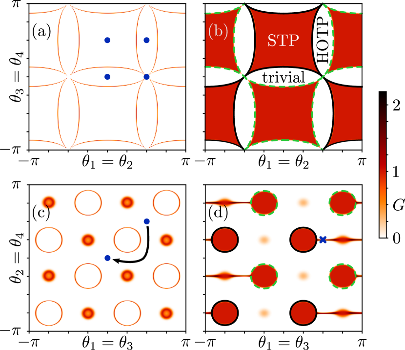
Figure 3: The dimensionless conductance $G$, computed for a network of $20\times 20$ unit cells, is plotted as a function of the angles $\theta_{1}=\theta_{2}$ and $\theta_{3}=\theta_{4}$ ($C_{4}$ symmetric) in panels (a) and (b). Similarly, panels (c) and (d) show the case with $\theta_{1}=\theta_{3}$ and $\theta_{2}=\theta_{4}$ (broken $C_{4}$ symmetry). Note that in panels (a) and (c) we use periodic boundary conditions, whereas in panels (b) and (d) are computed using open boundary conditions. The black solid and green dashed lines denote the gap closings at $\bm{k}=(0,0)$ and $(\pi,\pi)$, respectively. The four blue dots in panel (a) mark the decoupled limits of Fig. 2. The two blue dots in panel (c) indicate the trivial (all $\theta=0$) and HOTP (all $\theta=\pi/2$) decoupled limits. The black arrow connecting them is an example of a $C_{4}$ symmetry breaking path in parameter space that allows to transition from the HOTP to the trivial phase without closing of the bulk gap. The blue cross in panel (d) shows a point at which only the top and bottom edges of the network conduct.

IV Phase diagram

We determine the phase diagram of the network model by computing its two-terminal dimensionless conductance $G$, given by the total transmission probability. To this end, we attach semi-infinite leads composed of Majorana modes to its left and right boundaries and calculate the two-lead scattering matrix associated to the whole network (see Appendix B for details). We consider systems with either OBC or with periodic boundary conditions (PBC) in the transverse direction. This enables us to distinguish between bulk and edge contributions to the two-terminal transmission probability.

We begin by preserving the $C_{4}$ symmetry and determining the phase diagram in the $\theta_{1}$–$\theta_{3}$ plane, shown in Figs. 3(a) and 3(b). We observe that the trivial phase and the HOTP have a vanishing two-terminal transmission probability $G$ for both OBC and PBC. The reason is that both the bulk and the edges are gapped. There are four topologically trivial regions in the $\theta_{1}$–$\theta_{3}$ plane, appearing as horizontally elongated regions of $G=0$ in Fig. 3(b), centered around $\theta_{3}=0,\pi$. The four HOTP regions appear in the same panel as vertically elongated $G=0$ regions centered around $\theta_{1}=\pm\pi/2$.

Additionally, we observe a total of four regions of STP, which show a quantized value $G=1$ with OBC, Fig. 3(b), but $G=0$ when imposing PBC, Fig. 3(a). This is consistent with edge transport due to the presence of a single chiral edge mode. Notice how the decoupled limits shown in Fig. 2 correspond to the centers of the HOTP, trivial phase, and STP regions, with the Majorana flat band of Fig. 2(d) forming a critical point at which the three phases meet. The position of these phases relative to each other in parameter space is a consequence of several symmetries of the Ho-Chalker operator, as we explain in Appendix C.

Along the phase transition lines, the bulk gap around $\varepsilon=0$ closes, as do all of the other gaps (at $\varepsilon=\pm\pi/2$, $\pi$) related to it by the phase-rotation symmetry. The gap closing condition is given by

$$\det\Biggl{(}\prod_{j=1}^{4}{\cal S}_{j}-\mathbbm{1}_{4\times 4}\Biggr{)}=0,$$ (11)

with solutions of the form

$$|\cos\theta_{1}\mp\sin\theta_{3}|=\sqrt{2}|\sin\theta_{3}\cos\theta_{1}|,$$ (12)

at $\bm{k}=(0,0)$ and $\bm{k}=(\pi,\pi)$, respectively. Note that the two solutions, shown as solid black and dashed green lines in Fig. 3(b), nicely match the numerics.

In Figs. 3(a) and 3(b), there is no path in the phase diagram which connects the HOTP to the trivial phase without a bulk gap closing. As discussed in the previous section, this is a consequence of $C_{4}$ symmetry, which forbids the dimerization of corner modes along the edges of the system. Conversely, if $C_{4}$ symmetry is broken, it becomes possible to connect the HOTP and trivial phase while preserving the bulk gap. We explore this possibility in Figs. 3(c) and 3(d), where the transmission probability is plotted as a function of $\theta_{1}=\theta_{3}$ and $\theta_{2}=\theta_{4}$. These two axes correspond to different dimerizations between Majorana loops of the network in the horizontal and vertical directions, analogous to how dimerization can be varied independently for the horizontal and vertical hoppings of the BBH model (see Appendix A).

Along the diagonals of Fig. 3(c), $\theta_{1}=\theta_{2}$ and $\theta_{1}=-\theta_{2}$, a $C_{4}$ symmetry is preserved (albeit with a different symmetry operator; see Appendix D). When all $\theta$s are equal, there is an intermediate STP centered around $\theta=\pi/4$ which separates the trivial phase ($\theta=0$) and HOTP ($\theta=\pi/2$). In this case, the analytical expression for the gap closing is given by $|\sin(\pi/4\pm\theta_{1})\sin(\pi/4\pm\theta_{2})|=\sqrt{3}/2$ at ${\bm{k}}=(0,0),(\pi,\pi)$. The corresponding contours are shown as black solid and green dashed lines in Fig. 3(d). Note that along the antidiagonal with $\theta_{1}=-\theta_{2}$, the system remains trivial. However, we observe bulk gap closings at the points $(\theta_{1},\theta_{2})=(\pi/4,-\pi/4)$ and $(-\pi/4,\pi/4)$ [corresponding to $\bm{k}=(0,\pi)$ and $(\pi,0)$]. These are visible as small spots of increased transmission probability in the numerical data of Fig. 3(c).

Away from the diagonal, there exists a continuous path, shown as a black arrow in Fig. 3(c), which connects the HOTP to the trivial phase without closing the bulk gap. Note that along this path the topology is changed by an edge gap closing. Indeed, for any path connecting the HOTP and trivial regions either the bulk or the edge gap must close, since the Majorana corner modes can only be gapped out by pairwise coupling. When adjacent corner modes hybridize through the top and bottom edges, they form counterpropagating edge modes which are visible in the transmission map of Fig. 3(d); for instance at $\theta_{1}=\pi/2$, $\theta_{2}=\pi/4$ (blue cross). In fact, the closing of the edge gap is the reason for the thin horizontal lines of Fig. 3(d) at which we observe $G=2$, consistent with the presence of counterpropagating edge modes on both the top and bottom edges. In contrast, corner modes overlapping via the left and right edges of the network (such as at the point $\theta_{1}=\pi/4$, $\theta_{2}=\pi/2$) do not contribute to transmission, since the leads are attached to the left and right sides of the network and thus we only probe transport along the top and bottom edges.

Note that at the point $(\theta_{1},\theta_{2})=(\pi/4,\pi/4)$, the links of the network are maximally coupled, in the sense that each incoming Majorana mode has an equal probability of turning clockwise or counterclockwise at each node of the network. In the CC model and, as far as we know, in all of its generalizations (Evers and Mirlin, 2008; Kagalovsky et al., 1999; Chalker et al., 2001; Fulga et al., 2012a; Obuse et al., 2014; Beamond et al., 2002; Obuse et al., 2007; Pasek and Chong, 2014; Son and Raghu, ), the maximally coupled limit is a gapless critical point separating topologically distinct phases. Interestingly, here it corresponds to a gapped, STP. For the parametrization shown in Figs. 3(c) and 3(d), in which $\theta_{1}=\theta_{3}$ and $\theta_{2}=\theta_{4}$, the point $(\theta_{1},\theta_{2})=(\pi/4,\pi/4)$ is in the middle of the strong topological region of the phase diagram, at which the bulk gap is the largest.

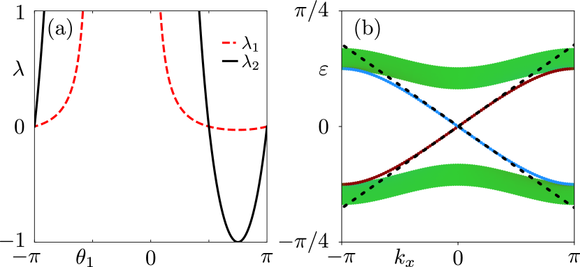
Figure 4: (a) Decay parameters as a function of $\theta_{1}$ at $\theta_{2}=\pi/4$. Note that the number of solutions with $\lambda<1$ correspond to the number of edge modes present. (b) Bandstructure of the network model at the maximally coupled point, $(\theta_{1},\theta_{2})=(\pi/4,\pi/4)$, computed in a ribbon geometry, infinite in the horizontal direction and consisting of 20 unit cells in the vertical direction. The bulk states are shown in green, whereas red and blue colors denote modes localized on the top and bottom boundaries, respectively. The dashed black lines show the velocities $v_{E}=\pm\sqrt{2}/8$ which is the perturbative expression valid for small wavenumbers.

To gain insight into the behavior of the network in the vicinity of $(\theta_{1},\theta_{2})=(\pi/4,\pi/4)$, we study a half-plane geometry (on $y<0$). We use an ansatz wavefunction $\Phi_{\rm tot}=(\Phi,\lambda\Phi,\lambda^{2}\Phi,\cdots)^{T}$ for the edge state, with a decay factor $\lambda$ between successive unit cells along the $y$ direction. The eigenvalue equation yielding stationary states then becomes

$$[\mathcal{S}_{0}(k_{x})+\lambda\mathcal{S}^{{}^{\prime}}]\Phi =e^{-i\varepsilon(k_{x})}\Phi,$$ (13)

$$[\lambda^{-1}\mathcal{S}^{{}^{\prime\prime}}+\mathcal{S}(k_{x})+\lambda\mathcal{S}^{{}^{\prime}}]\Phi =e^{-i\varepsilon(k_{x})}\Phi,$$ (14)

where $\mathcal{S}_{0}(k_{x})$ and $\mathcal{S}(k_{x})$ represent scattering terms within each unit cell, located at the boundary of the network ($y=0$) and away from it, respectively. The two other Ho-Chalker operators $\mathcal{S}^{{}^{\prime}}$ and $\mathcal{S}^{{}^{\prime\prime}}$ represent coupling to the adjacent unit cells, located respectively below and above. As discussed before, the open boundary condition is implemented by having the scattering nodes on the edge of the system completely reflect the incoming waves with unit probability amplitude (this corresponds to setting $\theta_{3}=0$ for those particular nodes). Considering $\varepsilon(k_{x})=0$ and fixing one angle as $\theta_{2}=\pi/2$, we find two possible values for the decay constant, $\lambda_{\pm}=(\sqrt{2}\pm 1)^{2}\,\tan(\pi/4-\theta_{1}/2)/\tan(\theta_{1}/2)$ which are shown in Fig. 4(a). Since normalizable edge modes require $|\lambda|<1$, this criterion leads to one edge state for $\theta_{1}\in(\frac{1}{12}\pi,\frac{5}{12}\pi)\cup(-\frac{11}{12}\pi,-\frac{7}{12}\pi)$, and two counterpropagating edge states for $\theta_{1}\in(\frac{5}{12}\pi,\frac{13}{12}\pi)$. The ranges for $\theta_{1}$ correspond to the regions of the STP and the horizontal line of $G=2$ emanating from it, respectively, as shown in Fig. 3(d). Furthermore, by performing perturbation theory in $k_{x}$, we obtain the linear dispersion $\varepsilon(k_{x})=v_{E}k_{x}$, with the velocity $|v_{E}|=\sqrt{2}/8\approx 0.18$ of the edge state, see Fig. 4(b).

V Topological invariants

In this section, we classify the different topological phases realized by the network model using topological invariants based on the scattering matrix of the system. In the HOTP, this approach is augmented with a symmetry indicator analysis whenever possible.

We first discuss the HOTP with its limiting case shown in Fig. 2(a). Note that, as discussed in the previous section, phase transitions separating the trivial phase from the HOTP can occur either via a bulk gap closing or via an edge gap closing, depending on whether rotation symmetry is preserved or not. This marks a distinction between the topological phases classified as intrinsic and those classified as extrinsic in Ref. Geier et al. (2018). The intrinsic HOTPs host corner states due to bulk topological invariants enabled by lattice symmetries, and thus can only transition to a trivial phase by closing the bulk gap or by lattice symmetry breaking. In contrast, extrinsic HOTPs owe their topological midgap states to the strong nontrivial topology of the system’s surface. Thus, in an extrinsic HOTP, corner modes are robust against lattice symmetry breaking (e.g. due to disorder), provided that the surface gap does not close. As we shall see in the following, the network model we introduce has a dual topology: When rotation symmetry is preserved it realizes an intrinsic HOTP protected by a bulk invariant, and when rotation is broken it realizes an extrinsic HOTP which does not rely on lattice symmetries.

A set of topological invariants detecting the presence of corner modes can be found in a four-terminal geometry, in which one lead is attached to each of the corners of the system, as shown in Refs. Geier et al. (2018); Franca et al. (2019). We provide more details on this transport geometry in Appendix B. This setup only allows us to characterize the HOTP as an extrinsic topological phase Geier et al. (2018), as corner leads cannot distinguish between topology due to a nontrivial bulk and due to nontrivial edges.

In the HOTP, both bulk and edges are gapped, as exemplified in Fig. 2(a). As such, in each of the four corner leads, incoming modes are fully back-reflected and the corresponding corner reflection matrices $\mathfrak{r}_{j}$ ($j=1,2,3,4$) are unitary. Furthermore, the reflection blocks $\mathfrak{r}_{j}$ are also real due to particle-hole symmetry, leading to the $\mathbb{Z}_{2}$ invariants (Akhmerov et al., 2011; Fulga et al., 2012b)

$$\nu_{j}=\mathop{\rm sgn}\det\mathfrak{r}_{j}\,.$$ (15)

The values $\nu_{j}=\pm 1$ are topologically distinct since the only way to interpolate between them is by going through a point for which $\det{\mathfrak{r}_{j}}=0$, indicating that there is at least one fully transmitting mode connecting the leads at the different corners, either through the bulk or through the edges. Since in the HOTP the corner modes simultaneously appear at all four corners, we will only investigate $\mathfrak{r}_{1}$ in the following.

Conventionally, a value $\nu_{1}=1$ indicates the trivial phase and $\nu_{1}=-1$ the topological phase, due to the $\pi$ phase shift caused by the resonant reflection of waves on a zero-energy state (Akhmerov et al., 2011; Fulga et al., 2012b; Franca et al., 2019). However, the relation is exactly inverted in our model, cf. Fig. 2(a). In particular, we see that the loop containing the corner mode is periodic and thus does not lead to a $\pi$ phase shift. As a result, we find $\nu_{1}=1$ in the topological phase. Analogously, the invariant is $\nu_{1}=-1$ in the trivial phase, with decoupled limit shown in Fig. 2(b) due to the fact that the loop at the corner is antiperiodic. Therefore, $\nu_{1}=-1$ describes the trivial phase of the network model .

In Fig. 5, we show how $\det\mathfrak{r}_{1}$ depends on the angles $\theta_{1},\theta_{2},\theta_{3}$, and $\theta_{4}$. In Fig. 5(a), we consider the $C_{4}$ symmetric network model. We observe a good agreement with the phase diagram of Fig. 2(b), which has been obtained from the two-terminal transmission probability. The invariant correctly identifies the HOTP and trivial regions, while the STP regions have $\det\mathfrak{r}_{1}\approx 0$. However, the phase boundaries between the HOTP (or trivial phase) and the STP are not as easily seen as in the two terminal calculations. For this reason, we plot $1-|\det\mathfrak{r}_{1}|$ in Fig. 5(b), and look at small deviations from $0$. The resulting phase diagram is now in excellent agreement with Fig. 2(b).

Once $\theta_{1}=\theta_{3}$ and $\theta_{2}=\theta_{4}$, such that $C_{4}$ is broken, the system produces the phase diagram shown in Fig. 5(c). Comparing to Fig. 2(c), it differs significantly. The difference occurs because the two-terminal transmission probability is only sensitive to gap closings along one set of edges, while the four-terminal geometry detects gap closings along all edges. For this reason, in Fig. 2(c), we only observe the gap closings on the top and bottom edges, while Fig. 5(c) contains information on gap closings also on the left and right edges. Again the features are better visible in Fig. 5(d), where we plot $1-|\det\mathfrak{r}_{1}|$. We see that the HOTP is separated from the trivial phase by a gap closing either in the bulk or along the edges, as is characteristic of extrinsic topological phases.

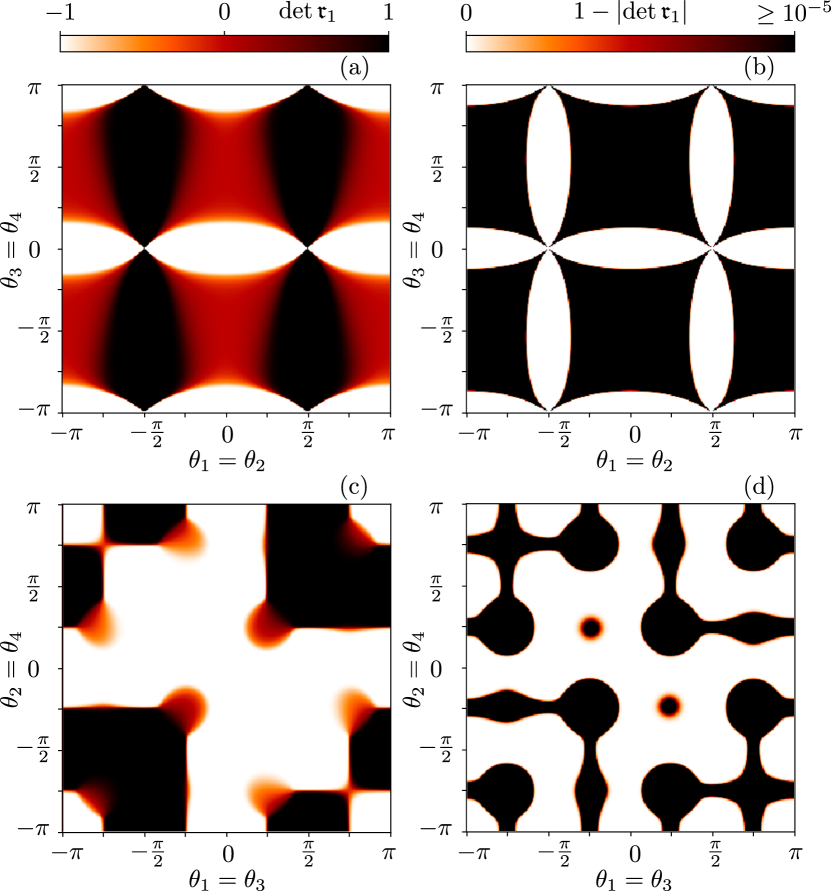
Figure 5: In panel (a), $\det\mathfrak{r}_{1}$ is plotted for $\theta_{1}=\theta_{2}$ and $\theta_{3}=\theta_{4}$. Panel (b) shows the deviation of $|\det\mathfrak{r}_{j}|$ from unity, such that the phase transitions are clearly visible. Panel (c) [(d)] depicts $\det\mathfrak{r}_{1}$ [$1-|\det\mathfrak{r}_{1}|$] for $\theta_{1}=\theta_{3}$ and $\theta_{2}=\theta_{4}$ such that the $C_{4}$ symmetry is broken.

In the presence of a $C_{4}$ symmetry, however, the HOTP is an intrinsic, bulk topological phase, such that a transition to a different phase requires the closing and reopening of the bulk (and not just the edge) gap Benalcazar et al. (2017b). To show this fact mathematically, we define a bulk $\mathbb{Z}_{2}$ topological invariant $Q=\pm 1$ based on the $C_{4}$ symmetry eigenvalues of the Ho-Chalker eigenstates for a translationally invariant system at the $C_{4}$ invariant points of Brillouin zone $\Gamma=(0,0)$ and $M=(\pi,\pi)$, similar to how this is done for static Hamiltonian systems Benalcazar et al. (2017b, 2019); Schindler et al. (2019); Geier et al. (2020); Roberts et al. (2020). It reads

$$\mathcal{Q}=d_{4}^{+}(M)d_{4}^{+}(\Gamma)^{*}=d_{4}^{-}(M)d_{4}^{-}(\Gamma)^{*},$$ (16)

where $d_{4}^{\pm}$ are the $\mathcal{C}_{4}$ eigenvalues that square to $\pm i$ in the ”occupied bands” of the Ho-Chalker operator. Even though the latter has a periodic spectrum, the phase-rotation and particle-hole symmetries enable us to unambiguously define the occupied bands as those in the interval $-\pi/4<\varepsilon<0$ (which is half of the fundamental phase domain).

Since the $C_{4}$ symmetry operator of Eq. (10) obeys $\mathcal{R}^{4}=-1$, its eigenvalues are $e^{\pm i\pi/4}$ and $e^{\pm i3\pi/4}$. In the HOTP, we find that the two occupied bands in the fundamental domain have eigenvalues $e^{-i\pi/4}$ and $e^{-i3\pi/4}$ at the $\Gamma$ point. At the $M$ point, these bands change their symmetry eigenvalues to $e^{i3\pi/4}$ and $e^{i\pi/4}$, respectively. We thus obtain $\mathcal{Q}=-1$ which corresponds to the HOTP. In the trivial phase, we find the $C_{4}$ symmetry indicators of occupied bands do not change between $\Gamma$ and $M$, which leads to a value of $\mathcal{Q}=1$.

Finally, the topological invariant of the STP can be expressed as the winding number Bräunlich et al. (2010); Fulga et al. (2012b); Fulga and Maksymenko (2016)

$$\mathcal{W}=\frac{1}{2\pi i}\int_{0}^{2\pi}\!d\varphi\,\frac{d}{d\varphi}\text{log}\>\text{det}\>\mathfrak{r}(\varphi),$$ (17)

where $\mathfrak{r}(\varphi)$ is the reflection block of the two-terminal scattering matrix. Here, we impose twisted boundary conditions in the vertical direction, with twist angle $\varphi$, such that $\varphi=0$ corresponds to PBC. We have checked that all phases of Fig. 3 in which $G=0$ with PBC and $G=1$ with OBC have $\mathcal{W}=-1$, confirming that they are indeed STPs.

VI Disorder

We study the effect of disorder on the network model by adding a random term $\delta\theta_{i}$ to each $\theta_{i}$, drawn uniformly for each angle from the uniform distribution $[-w,w]$, with the disorder strength $w$, $0\leq w\leq\pi$. The disorder breaks all lattice symmetries but preserves particle-hole symmetry since the disordered scattering matrices remain orthogonal. As the system is still in the class D, we expect that, with sufficiently strong disorder, the phase boundaries separating the HOTP, STP, and trivial phase will evolve into a delocalized phase similar to the ‘thermal metal’ which occurs in static disordered systems Evers and Mirlin (2008); Kagalovsky et al. (1999); Chalker et al. (2001); Cho and Fisher (1997); Medvedyeva et al. (2010); Fulga et al. (2020). In contrast, for weak disorder, the system should be insensitive to disorder, with only minor modifications of the phase diagram with respect to the clean case.

We verify this behavior by computing the average two-terminal transmission of the disordered network model. In Fig. 6, without disorder ($w=0$), we observe all three phases: trivial, STP, and HOTP. All of them have a localized bulk and thus are robust against disorder up to a moderate disorder strength, $w<1$. For the HOTP, this robustness is a consequence of the extrinsic nature of the topological phase. Even though the rotation symmetry enabling the bulk invariant Eq. (16) is broken, the particle-hole symmetric corner modes cannot be removed as long as the bulk and surfaces remain localized. However, as disorder strength is increased beyond $w\simeq 1$, each phase undergoes a bulk localization-delocalization transition, and its topological properties are lost.

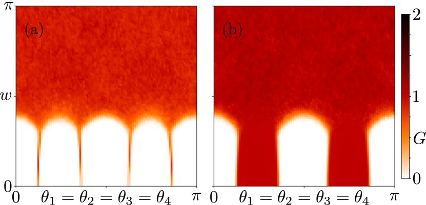
Figure 6: Dimensionless conductance $G$ computed for a network model with $20\times 20$ unit cells as a function of $w$ and $\theta_{i}$ ($i=1,2,3,4$) using PBC (a) and OBC (b). Each point is obtained by averaging over $100$ disorder realizations.

Next, we fix $w=1.1$ and in Fig. 7 plot the average transmission probability as a function of different $\theta$s, to show how the phase diagram of Fig. 3 changes in the presence of moderate disorder. Among the four decoupled limits of the clean $C_{4}$ symmetric case, the Majorana flat band is first to be delocalized due to its gapless bandstructure. In addition, the network model near the phase boundaries (or any other gap closing points) can also be easily delocalized, as seen in Figs. 7(a) and 7(b). As such, we observe that in the disordered phase diagram the phase transition lines separating HOTP, STP, and trivial phases evolve into finite-width delocalized regions, as do the gapless points at $(\theta_{1},\theta_{2})=(\pi/4,-\pi/4)$ and $(-\pi/4,\pi/4)$. Nevertheless, the STP and HOTP retain their nontrivial nature, despite the presence of disorder. The transmission probability still changes from $G=0$ with PBC to $G=1$ with OBC in the STP, signaling that the chiral Majorana edge mode is robust against disorder. We have confirmed that the scattering matrix invariants characterizing the HOTP and STP retain their nontrivial values. Finally, we observe that the counterpropagating edge modes separating HOTP and trivial phase in the $C_{4}$ broken case [Fig. 7(d)] remain conducting, albeit with a conductance $G<2$. In fact they are protected by an average translation symmetry of the ensemble of disorder realizations Brouwer et al. (2000, 2003); Fulga et al. (2014); Diez et al. (2014, 2015).

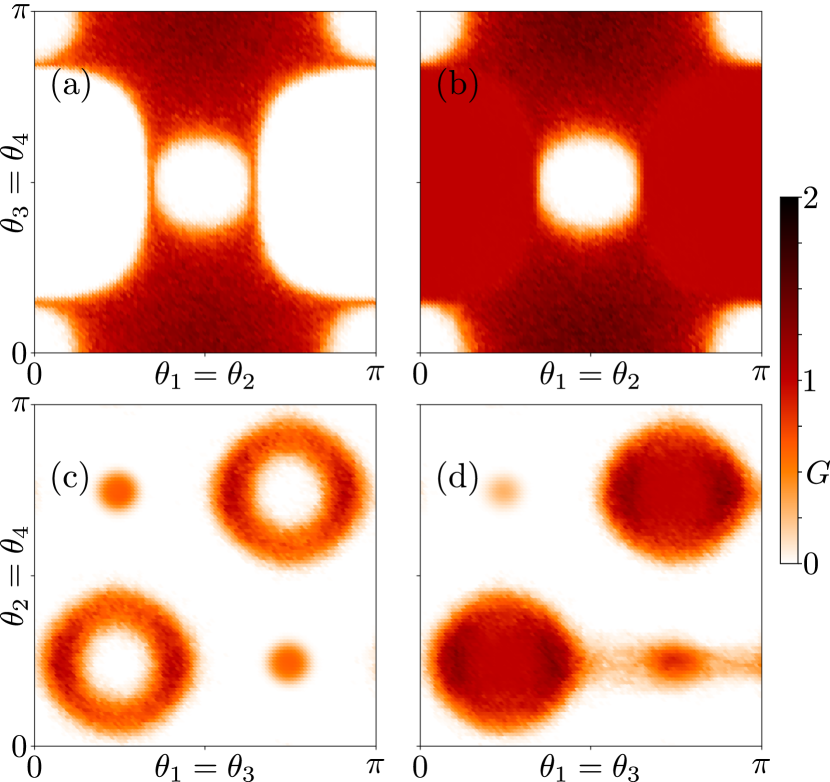
Figure 7: Dimensionless conductance $G$ as a function of $\theta_{1}=\theta_{2}$ and $\theta_{3}=\theta_{4}$ ($C_{4}$ symmetric) in panels (a) and (b), and as a function of $\theta_{1}=\theta_{3}$ and $\theta_{2}=\theta_{4}$ (broken $C_{4}$ symmetry) in panels (c) and (d). In panels (a) and (c), we use periodic boundary conditions, whereas panels (b) and (d) we use open boundary conditions. All plots are computed for a network model consisting of $50\times 50$ unit cells, with disorder strength $w=1.1$, and each point is obtained by averaging over 50 disorder realizations.

VII Network models in experiment

The first network model was introduced by Chalker and Coddington to describe the low-energy, course-grained physics of a static system: the quantum Hall effect Chalker and Coddington (1988). Unidirectional links represented chiral quantum Hall edge modes and the scattering centers were the saddle points of the chemical potential at which these edge modes mix. Using a similar language, we have introduced our particle-hole symmetric network model at the beginning of Sec. II in terms of chiral Majorana modes. These are connected to each other by scattering processes, as would occur in a static $p$-wave superconductor, for instance.

Network models, however, are dynamical systems. This fact, as pointed out in Refs. Janssen et al. (1999); Pasek and Chong (2014), is related to the unitary nature of the operator used to describe network models, the Ho-Chalker operator. The latter encodes all of the scattering processes acting on the network wavefunction, which can be modeled as a discrete-time evolution [see Eq. (3)]. Its eigenstates are the steady states of the network, those which preserve their shape even upon multiple scatterings [see Eq. (5)].

The understanding of the network model as a dynamical system has led to its experimental realization in different platforms, such as microwave circuits Hu et al. (2015), or systems of coupled photonic Hafezi et al. (2011); Afzal et al. (2020) and plasmonic Gao et al. (2016, 2018) ring resonators. Excitations propagate along the ring resonators (or along optical fibers, in the microwave circuit implementation), and have the chance of scattering to neighboring resonators (optical fibers), depending on the distance, or amount of coupling between them. The entire array can then be described by a matrix of scattering amplitudes (the Ho-Chalker operator), and the dynamical phases acquired by its steady states after they scatter represent the eigenphases of this matrix. This means that the eigenphases of a network model are experimentally tunable parameters, similar to how the energies of states can be tuned by varying the chemical potential of static systems. The eigenphases can be changed by altering the ratio between the wavelength of the photons (plasmons) and the length of the optical fiber (resonator). In fact, recent experiments managed to probe the network model over the entire range $\varepsilon\in[0,2\pi)$ Afzal et al. (2020). In practice, these measurements oftentimes involve directly visualizing states as they scatter through the network, similar to how Floquet topological phases are measured in photonic crystals El Hassan et al. (2019).

Finally, we note that the large degree of control available in meta-material platforms enables the experimental realization of network models subject to various constraints, including particle-hole symmetry. In a traditional condensed matter setup, the latter would require superconductivity, hence our discussion in terms of Majorana modes in Sec. II. On the network model level, however, particle-hole symmetry simply means that the scattering matrices are real. This can be ensured in experiment by coupling the optical fibers or ring resonators to each other such that each scattering process involves the same phase difference between incoming and outgoing waves. In fact, network models with particle-hole symmetric spectra have already been measured in Refs. Gao et al. (2016); Afzal et al. (2020).

VIII Conclusion

We have introduced a network model realization of a higher-order topological phase. The system shows many similarities to the HOTP present in static or periodically driven Hamiltonian systems, namely it hosts zero-modes localized at the corners, which are protected by the bulk and edge gaps due to a combination of a particle-hole symmetry and a fourfold rotation symmetry. However, the network model additionally features a phase-rotation symmetry. As a result, there are a total of 16 topologically protected corner states, more than for a fourfold symmetric static or Floquet system. The HOTP is robust against disorder, being characterized by nontrivial scattering matrix invariants as well as by a more conventional invariant based on symmetry indicators.

We hope that our work will motivate further theoretical and experimental research into network models. The latter (as well as HOTPs) have been successfully realized using optical fibers and coupled ring resonators Ozawa et al. (2019); Hafezi et al. (2011, 2013); Liang and Chong (2013). In some of these platforms it is also possible to directly measure the scattering matrix invariants Hu et al. (2015); Wang et al. (2017). Therefore, the HOTP network proposed here, and its invariants could be experimentally probed in these platforms. Finally, our work provides an example of a network model for a point group symmetry protected topological phase. These are by now the most studied types of topology in condensed-matter, Hamiltonian systems, but have not yet been explored on the level of network models. We believe that different types of topological crystalline phases protected by different lattice symmetries may be realized using arrays of scattering matrices, and we plan to further explore this direction in the future.

Appendix A BBH Model

In this section, we briefly review the main features of the BBH model and explain its similarities to our network model.

The BBH model consists of noninteracting spinless electrons hopping on a square lattice. Only the nearest-neighbor hoppings are nonzero, and they are staggered in both directions, consisting of alternating weak and strong hopping strengths, as shown in Fig. 8(a). A magnetic $\pi$-flux pierces each plaquette, ensuring that the bulk and edges are gapped.

The momentum-space Hamiltonian reads

$$\begin{split}h(\bm{k})=&(\gamma_{x}+\lambda_{x}\cos{k_{x}})\tau_{x}\sigma_{0}-\lambda_{x}\sin{k_{x}}\tau_{y}\sigma_{z}\\ &-(\gamma_{y}+\lambda_{y}\cos{k_{y}})\tau_{y}\sigma_{y}-\lambda_{y}\sin{k_{y}}\tau_{y}\sigma_{x}.\end{split}$$ (18)

Here, $\bm{k}=(k_{x},k_{y})$ are the two momenta and Pauli matrices $\tau$ and $\sigma$ represent the sublattice degree of freedom and the site degree of freedom, respectively. Intracell hoppings are $\gamma_{x}$ and $\gamma_{y}$, while $\lambda_{x}$ and $\lambda_{y}$ denote intercell couplings.

Figure 8: (a) Sketch of the BBH model. The black dots represent sites. The intracell/intercell hoppings are shown in red/blue, respectively, and dashed lines denote negative hopping strengths (used to implement the $\pi$ fluxes). The gray rectangle depicts a unit cell. (b) Phase diagram of the BBH model Eq. (18). The gray area indicates the HOTP, while the red circles denote the points of the bulk gap closings. Moreover, the gap closings along the $x$- and $y$-edges are shown in blue and green, respectively. The arrows indicate possible paths in parameter space that lead to bulk gap (red), $x$-edge (blue) and $y$-edge (green) gap closings.

The system has a particle-hole symmetry $\mathcal{P}=\tau_{z}{\cal K}$, where ${\cal K}$ denotes complex-conjugation. Once $\gamma_{x}=\gamma_{y}\equiv\gamma$ and $\lambda_{x}=\lambda_{y}\equiv\lambda$, the system is $C_{4}$ symmetric. It obeys $\mathcal{R}h(k_{x},k_{y})\mathcal{R}^{-1}=h(k_{y},-k_{x})$, where the $C_{4}$ symmetry operator reads Benalcazar et al. (2017a)

$$\mathcal{R}=\begin{pmatrix}0&\sigma_{0}\\ -i\sigma_{y}&0\end{pmatrix}.$$ (19)

We now discuss the similarities between the BBH model and network model, and focus first on the $C_{4}$ symmetric limit. If the intracell coupling strength is much weaker than intercell coupling strength, then both systems with open boundaries would support four topologically protected zero-energy corner states. Then, in the opposite limit, both systems would also yield a trivially gapped bulk. Furthermore, for the BBH model, the bulk gap closing point is at $\bm{k}=(0,0)$ [$\bm{k}=(\pi,\pi)$] and occurs when $\gamma=-\lambda$ [$\gamma=\lambda$], as shown on Fig. 8(b). Similarly, the network model also possesses two types of gap closing at $\bm{k}=(0,0)$ and $\bm{k}=(\pi,\pi)$, shown in Fig. 3.

Once the $C_{4}$ symmetry is broken, the BBH model Eq. (18) is in a HOTP as long as $\gamma_{x}<\lambda_{x}$ and $\gamma_{y}<\lambda_{y}$. As denoted in Fig. 8(b), the phase without corner states can be reached by the $x$-edge gap closing ($\gamma_{x}=\lambda_{x}$) or the $y$-edge gap closing ($\gamma_{y}=\lambda_{y}$). The consequence of the edge gap closing is the appearance of two counterpropagating modes per edge. Then in the network model, once the $C_{4}$ symmetry is broken, the system is also in a HOTP as long as this phase does not reach edge gap closing lines, which correspond to a counterpropagating modes with $G=2$, see Figs. 3(d), 5(c), and 5(d).

Appendix B Transport geometries

In this section, we detail two transport geometries used for obtaining the phase diagrams in Figs. 3 and 5, respectively. We attach the code used to perform these calculations as an ancillary file.

For the conductance calculations in Fig. 2, we use two semi-infinite leads attached to opposite vertical edges of the 2D system, as shown in Fig. 9(a). Each lead is composed of an array of Majorana modes, thus preserving particle-hole symmetry. As such, in the Majorana basis the scattering matrix is real, and it has a size of $4N_{y}\times 4N_{y}$ for an $N_{x}\times N_{y}$ unit cell system. To compute this scattering matrix, we consider that the system consists of a sequence of 1D slices, as shown for a $2\times 2$ system in Fig. 9(a). Each slice contains an array of scattering nodes arranged vertically. Every slice has $4N_{y}$ incoming/outgoing modes, related by the scattering matrix

$$S_{\rm slice}=\begin{pmatrix}\mathfrak{r}_{\rm slice}&\mathfrak{t}_{\rm slice}^{\prime}\\ \mathfrak{t}_{\rm slice}&\mathfrak{r}_{\rm slice}^{\prime}\end{pmatrix},$$ (20)

where $\mathfrak{r}_{\rm slice}$ and $\mathfrak{r}_{\rm slice}^{\prime}$ are reflection matrices of the slice from left to left and from right to right, respectively. The transmission matrix from left to right, and vice versa are denoted by $\mathfrak{t}_{\rm slice}$ and $\mathfrak{t}_{\rm slice}^{\prime}$.

The final scattering matrix of the full network is obtained by combining scattering matrices of all $2N_{x}$ slices. If we label the scattering matrices for two adjacent slices as $S_{L}$ (left) and $S_{R}$ (right), respectively, then the scattering matrix $S_{C}$ of the new slice after combination has matrix blocks 

$$\begin{split}&\mathfrak{r}_{C}=\mathfrak{r}_{L}+\mathfrak{t}_{L}^{\prime}\mathfrak{r}_{R}(1-\mathfrak{r}_{L}^{\prime}\mathfrak{r}_{R})^{-1}\mathfrak{t}_{L},\\ &\mathfrak{t}_{C}=\mathfrak{t}_{R}(1-\mathfrak{r}_{L}^{\prime}\mathfrak{r}_{R})^{-1}\mathfrak{t}_{L},\\ &\mathfrak{t}_{C}^{\prime}=\mathfrak{t}_{L}^{\prime}(1-\mathfrak{r}_{R}\mathfrak{r}_{L}^{\prime})^{-1}\mathfrak{t}_{R}^{\prime},\\ &\mathfrak{r}_{C}^{\prime}=\mathfrak{r}_{R}^{\prime}+\mathfrak{t}_{R}\mathfrak{r}_{L}^{\prime}(1-\mathfrak{r}_{R}\mathfrak{r}_{L}^{\prime})^{-1}\mathfrak{t}_{R}^{\prime}.\end{split}$$ (21)

Therefore, after multiple combination processes, one can gradually include all slices and obtain the combined scattering matrix for the whole system. With this, we can calculate the conductance as $G=\text{tr}(\mathfrak{t}\mathfrak{t}^{\dagger})$, where $\mathfrak{t}$ is the transmission block of the full, two-terminal scattering matrix: $S_{\rm 2-term}$.

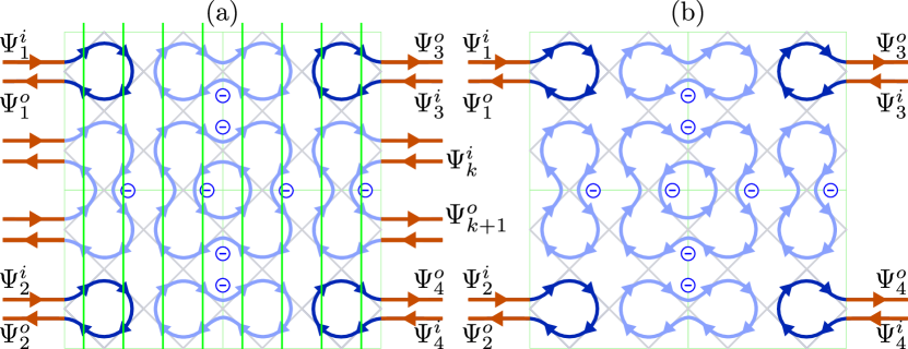
Figure 9: In panel (a) we show the two-terminal transport geometry. For simplicity, we consider a $N_{x}\times N_{y}=2\times 2$ system in a HOTP. The lead modes are depicted in red. The modes at corners are indexed with $k=1,2,3,4$, while all other modes are represented with $k$ $(k>4)$. The vertical green lines mark the different 1D slices which are combined to yield the full scattering matrix (see text). In panel (b), we show the four-terminal transport geometry with the leads only connected to the corners of the system.

For the calculation of the topological invariant $\nu_{1}$ to capture the presence of corner modes, we use a four-terminal geometry depicted in Fig. 9(b). The associated scattering matrix, $S_{\rm 4-term}$, can be calculated from $S_{\rm 2-term}$ in the following manner. We reorder the incoming and outgoing modes of $S_{\rm 2-term}$ such that it has the structure

$$S_{\rm 2-term}=\begin{pmatrix}S_{A}&S_{B}\\ S_{C}&S_{D}\end{pmatrix}.$$ (22)

Here, $S_{A}$ is a $4\times 4$ matrix that relates four corner incoming and outgoing modes, denoted in Fig. 9(b). Therefore $(\Psi_{1}^{o},\Psi_{2}^{o},\Psi_{3}^{o},\Psi_{4}^{o})^{T}=S_{A}(\Psi_{1}^{i},\Psi_{2}^{i},\Psi_{3}^{i},\Psi_{4}^{i})^{T}$. In general, $S_{A}$ is not necessarily a unitary matrix as the corner incoming modes can contribute to the outgoing modes not pinned at corners. Matrix $S_{B}$ has $4\times(4N_{y}-4)$ entries, and relates four outgoing corner modes with all remaining incoming amplitudes, while $S_{C}$ does the opposite. Finally, the matrix $S_{D}$ has $(4N_{y}-4)\times(4N_{y}-4)$ entries, and relates all noncorner incoming to noncorner outgoing modes.

To remove leads from the $x$-edges of the network model, except at the points of corner terminals, we assume $\Psi^{i}_{k}=\Psi_{k}^{o}$, for $4<k<4N_{y}$. Then, solving the set of these $4N_{y}-4$ number of equations, we can eliminate all but four incoming/outgoing modes. The resulting scattering matrix reads

$$S_{\rm 4-term}=S_{A}+S_{B}(1-S_{D})^{-1}S_{C}.$$ (23)

Appendix C Symmetries of the network model

We discuss here how different symmetries of the Ho-Chalker operator can be used to fully characterize the phase diagram discussed in the main text.

In the Ho-Chalker operator, each nonzero element is proportional to either $\sin\theta_{i}$ or $\cos\theta_{i}$ ($i=1,2,3,4$). This leads to

$$\mathcal{S}(\theta_{1},\theta_{2},\theta_{3},\theta_{4})=-\mathcal{S}(\theta_{1}+\pi,\theta_{2}+\pi,\theta_{3}+\pi,\theta_{4}+\pi).$$ (24)

The minus sign corresponds to a $\pi$ shift of all eigenphases, which, together with the $\pi/2$ shift caused by phase-rotation symmetry, means that both $\mathcal{S}(\theta_{1},\theta_{2},\theta_{3},\theta_{4})$ and $\mathcal{S}(\theta_{1}+\pi,\theta_{2}+\pi,\theta_{3}+\pi,\theta_{4}+\pi)$ have identical spectra and therefore share the same topological properties.

Another symmetry constraining the phase diagram is

$$U_{1}\mathcal{S}(\theta_{1},\theta_{2},\theta_{3},\theta_{4})U_{1}^{\dagger}=\mathcal{S}(-\theta_{1},-\theta_{2},\theta_{3},\theta_{4})$$ (25)

with $U_{1}=\mathbbm{1}_{4\times 4}\otimes{\rm diag}(1,1,-1,1)$. Because $\mathcal{S}(\theta_{1},\theta_{2},\theta_{3},\theta_{4})$ and $\mathcal{S}(-\theta_{1},-\theta_{2},\theta_{3},\theta_{4})$ have identical spectra, they are in the same topological phase.

Next, one can find that

$$\mathcal{S}(\theta_{1},\theta_{2},\theta_{3},\theta_{4},k_{x},k_{y})\\ =\mathcal{S}(\theta_{1},\theta_{2},-\theta_{3},-\theta_{4},k_{x}+\pi,k_{y}+\pi).$$ (26)

Therefore, these two systems are also in the same topological class: STP, HOTP, or trivial.

Finally, we introduce a fourth symmetry,

$$U_{2}\mathcal{S}(\theta_{1},\theta_{2},\theta_{3},\theta_{4})U_{2}^{\dagger}=\mathcal{S}(\theta_{1}+\pi,\theta_{2}+\pi,-\theta_{3},-\theta_{4}),$$ (27)

where

$$U_{2}=\begin{pmatrix}1&0&0&0\\ 0&-1&0&0\\ 0&0&1&0\\ 0&0&0&-1\end{pmatrix}\otimes\begin{pmatrix}1&0&0&0\\ 0&-1&0&0\\ 0&0&-1&0\\ 0&0&0&-1\end{pmatrix}.$$ (28)

Taken together, the symmetries listed above help to explain how the different topological phases of Fig. 3 are related to each other.

Appendix D $C_{4}$ symmetry when $\theta_{1}=\theta_{3}=-\theta_{2}=-\theta_{4}$

Along the diagonal line of $\theta_{1}=-\theta_{2}$ in Figs. 3(c) and 3(d), the system still preserves $C_{4}$ symmetry, but the $C_{4}$ symmetry condition becomes,

$$\mathcal{R}^{\prime}\mathcal{S}(k_{x},k_{y})\mathcal{R}^{\prime\dagger}=\mathcal{S}(-k_{y}+\pi,k_{x}+\pi),$$ (29)

with

$${\cal R}^{\prime}=\begin{pmatrix}0&0&0&\!{\cal R}^{\prime}_{4}\\ \!{\cal R}^{\prime}_{3}\!&0&0&0\\ 0&\!{\cal R}^{\prime}_{2}\!&0&0\\ 0&0&\!{\cal R}^{\prime}_{1}\!&0\end{pmatrix}\!,\;{\cal R}^{\prime}_{i}=K_{i}\begin{pmatrix}1&0&0&0\\ 0&0&0&1\\ 0&0&-1&0\\ 0&1&0&0\end{pmatrix}\!,$$ (30)

with the $K_{i}$ matrices defined as in Eq. (10). If momentum space is discretized (for instance in a torus geometry), then this symmetry constraint needs an even number of discretized momenta $k_{x}$ and $k_{y}$ to be preserved. Correspondingly, in real space the rotation axis is positioned at the corner of the unit cell.

At the two high symmetry points $X=(\pi,0)$ and $Y=(0,\pi)$ we have $[\mathcal{R}^{\prime},\mathcal{S}]=0$ in momentum space. Like Section V, we can again determine the $C_{4}$ eigenvalues of the occupied bands. Since $(\mathcal{R}^{\prime})^{4}=-1$, these eigenvalues are $e^{\pm i\pi/4}$ and $e^{\pm i3\pi/4}$. When changing $\theta_{1}=-\theta_{2}$ so as to move on the diagonal of Fig. 3(c), we observe that there is a bulk gap closing and reopening which occurs at the point $\pi/4$. This gap closing is parabolic as a function of the $\theta$s, and so does not involve a band inversion in which states with different $C_{4}$ eigenvalues cross $\varepsilon=0$ and are interchanged. As such, no topological phase transition takes place at $\theta_{1}=-\theta_{2}=\pi/4$.

References

- Schnyder et al. (2008) Andreas P. Schnyder, Shinsei Ryu, Akira Furusaki, and Andreas W. W. Ludwig, “Classification of topological insulators and superconductors in three spatial dimensions,” Phys. Rev. B 78, 195125 (2008).
- Ryu et al. (2010) Shinsei Ryu, Andreas P Schnyder, Akira Furusaki, and Andreas W. W. Ludwig, “Topological insulators and superconductors: tenfold way and dimensional hierarchy,” New J. Phys. 12, 065010 (2010).
- Chiu et al. (2016) Ching-Kai Chiu, Jeffrey C. Y. Teo, Andreas P. Schnyder, and Shinsei Ryu, “Classification of topological quantum matter with symmetries,” Rev. Mod. Phys. 88, 035005 (2016).
- Mong et al. (2010) Roger S. K. Mong, Andrew M. Essin, and Joel E. Moore, “Antiferromagnetic topological insulators,” Phys. Rev. B 81, 245209 (2010).
- Fu (2011) Liang Fu, “Topological crystalline insulators,” Phys. Rev. Lett. 106, 106802 (2011).
- Slager et al. (2013) Robert-Jan Slager, Andrej Mesaros, Vladimir Juričić, and Jan Zaanen, “The space group classification of topological band-insulators,” Nat. Phys. 9, 98 (2013).
- Ando and Fu (2015) Yoichi Ando and Liang Fu, “Topological crystalline insulators and topological superconductors: From concepts to materials,” Annu. Rev. Condens. Matter Phys. 6, 361 (2015).
- Chiu et al. (2013) Ching-Kai Chiu, Hong Yao, and Shinsei Ryu, “Classification of topological insulators and superconductors in the presence of reflection symmetry,” Phys. Rev. B 88, 075142 (2013).
- Benalcazar et al. (2017a) Wladimir A. Benalcazar, B. Andrei Bernevig, and Taylor L. Hughes, “Quantized electric multipole insulators,” Science 357, 61 (2017a).
- Benalcazar et al. (2017b) Wladimir A. Benalcazar, B. Andrei Bernevig, and Taylor L. Hughes, “Electric multipole moments, topological multipole moment pumping, and chiral hinge states in crystalline insulators,” Phys. Rev. B 96, 245115 (2017b).
- Langbehn et al. (2017) Josias Langbehn, Yang Peng, Luka Trifunovic, Felix von Oppen, and Piet W. Brouwer, “Reflection-symmetric second-order topological insulators and superconductors,” Phys. Rev. Lett. 119, 246401 (2017).
- Song et al. (2017) Zhida Song, Zhong Fang, and Chen Fang, “-dimensional edge states of rotation symmetry protected topological states,” Phys. Rev. Lett. 119, 246402 (2017).
- Schindler et al. (2018a) Frank Schindler, Zhijun Wang, Maia G Vergniory, Ashley M Cook, Anil Murani, Shamashis Sengupta, Alik Yu Kasumov, Richard Deblock, Sangjun Jeon, Ilya Drozdov, et al., “Higher-order topology in bismuth,” Nat. Phys. 14, 918 (2018a).
- Schindler et al. (2018b) Frank Schindler, Ashley M. Cook, Maia G. Vergniory, Zhijun Wang, Stuart S. P. Parkin, B. Andrei Bernevig, and Titus Neupert, “Higher-order topological insulators,” Sci. Adv. 4, 0346 (2018b).
- Geier et al. (2018) Max Geier, Luka Trifunovic, Max Hoskam, and Piet W. Brouwer, “Second-order topological insulators and superconductors with an order-two crystalline symmetry,” Phys. Rev. B 97, 205135 (2018).
- Khalaf (2018) Eslam Khalaf, “Higher-order topological insulators and superconductors protected by inversion symmetry,” Phys. Rev. B 97, 205136 (2018).
- Trifunovic and Brouwer (2019) Luka Trifunovic and Piet W. Brouwer, “Higher-order bulk-boundary correspondence for topological crystalline phases,” Phys. Rev. X 9, 011012 (2019).
- Wang et al. (2018a) Yuxuan Wang, Mao Lin, and Taylor L. Hughes, “Weak-pairing higher order topological superconductors,” Phys. Rev. B 98, 165144 (2018a).
- van Miert and Ortix (2018) Guido van Miert and Carmine Ortix, “Higher-order topological insulators protected by inversion and rotoinversion symmetries,” Phys. Rev. B 98, 081110 (2018).
- You et al. (2018) Yizhi You, Trithep Devakul, F. J. Burnell, and Titus Neupert, “Higher-order symmetry-protected topological states for interacting bosons and fermions,” Phys. Rev. B 98, 235102 (2018).
- Călugăru et al. (2019) Dumitru Călugăru, Vladimir Juričić, and Bitan Roy, “Higher-order topological phases: A general principle of construction,” Phys. Rev. B 99, 041301 (2019).
- Araki et al. (2019) Hiromu Araki, Tomonari Mizoguchi, and Yasuhiro Hatsugai, “Phase diagram of a disordered higher-order topological insulator: A machine learning study,” Phys. Rev. B 99, 085406 (2019).
- Kudo et al. (2019) Koji Kudo, Tsuneya Yoshida, and Yasuhiro Hatsugai, “Higher-order topological Mott insulators,” Phys. Rev. Lett. 123, 196402 (2019).
- Tiwari et al. (2020) Apoorv Tiwari, Ming-Hao Li, B. A. Bernevig, Titus Neupert, and S. A. Parameswaran, “Unhinging the surfaces of higher-order topological insulators and superconductors,” Phys. Rev. Lett. 124, 046801 (2020).
- Ezawa (2018a) Motohiko Ezawa, “Higher-order topological insulators and semimetals on the breathing Kagome and pyrochlore lattices,” Phys. Rev. Lett. 120, 026801 (2018a).
- Ezawa (2018b) Motohiko Ezawa, “Minimal models for Wannier-type higher-order topological insulators and phosphorene,” Phys. Rev. B 98, 045125 (2018b).
- Hsu et al. (2018) Chen-Hsuan Hsu, Peter Stano, Jelena Klinovaja, and Daniel Loss, “Majorana Kramers pairs in higher-order topological insulators,” Phys. Rev. Lett. 121, 196801 (2018).
- Wang et al. (2018b) Qiyue Wang, Cheng-Cheng Liu, Yuan-Ming Lu, and Fan Zhang, “High-temperature Majorana corner states,” Phys. Rev. Lett. 121, 186801 (2018b).
- Yan et al. (2018) Zhongbo Yan, Fei Song, and Zhong Wang, “Majorana corner modes in a high-temperature platform,” Phys. Rev. Lett. 121, 096803 (2018).
- Ghorashi et al. (2020a) Sayed Ali Akbar Ghorashi, Tianhe Li, and Taylor L. Hughes, “Higher-order Weyl semimetals,” Phys. Rev. Lett. 125, 266804 (2020a).
- Ghorashi et al. (2020b) Sayed Ali Akbar Ghorashi, Taylor L. Hughes, and Enrico Rossi, “Vortex and surface phase transitions in superconducting higher-order topological insulators,” Phys. Rev. Lett. 125, 037001 (2020b).
- Ghorashi et al. (2019) Sayed Ali Akbar Ghorashi, Xiang Hu, Taylor L. Hughes, and Enrico Rossi, “Second-order Dirac superconductors and magnetic field induced Majorana hinge modes,” Phys. Rev. B 100, 020509 (2019).
- Note (1) Even though the BBH model is probably well known by now, we briefly summarize its main features and compare it with our network model in Appendix A.
- Serra-Garcia et al. (2018) Marc Serra-Garcia, Valerio Peri, Roman Süsstrunk, Osama R Bilal, Tom Larsen, Luis Guillermo Villanueva, and Sebastian D Huber, “Observation of a phononic quadrupole topological insulator,” Nature 555, 342 (2018).
- Peterson et al. (2018) Christopher W. Peterson, Wladimir A. Benalcazar, Taylor L. Hughes, and Gaurav Bahl, “A quantized microwave quadrupole insulator with topologically protected corner states,” Nature 555, 346 (2018).
- Imhof et al. (2018) Stefan Imhof, Christian Berger, Florian Bayer, Johannes Brehm, Laurens W Molenkamp, Tobias Kiessling, Frank Schindler, Ching Hua Lee, Martin Greiter, Titus Neupert, et al., “Topolectrical-circuit realization of topological corner modes,” Nat. Phys. 14, 925 (2018).
- Serra-Garcia et al. (2019) Marc Serra-Garcia, Roman Süsstrunk, and Sebastian D. Huber, “Observation of quadrupole transitions and edge mode topology in an LC circuit network,” Phys. Rev. B 99, 020304 (2019).
- Zhang et al. (2019) Xiujuan Zhang, Hai-Xiao Wang, Zhi-Kang Lin, Yuan Tian, Biye Xie, Ming-Hui Lu, Yan-Feng Chen, and Jian-Hua Jiang, “Second-order topology and multidimensional topological transitions in sonic crystals,” Nat. Phys. 15, 582 (2019).
- Kempkes et al. (2019) S. N. Kempkes, M. R. Slot, J. J. van Den Broeke, P. Capiod, W. A. Benalcazar, D. Vanmaekelbergh, D. Bercioux, I. Swart, and C. Morais Smith, “Robust zero-energy modes in an electronic higher-order topological insulator,” Nat. Mater. 18, 1292 (2019).
- Yue et al. (2019) Changming Yue, Yuanfeng Xu, Zhida Song, Hongming Weng, Yuan-Ming Lu, Chen Fang, and Xi Dai, “Symmetry-enforced chiral hinge states and surface quantum anomalous hall effect in the magnetic axion insulator bi2-xsmxse3,” Nature Physics 15, 577–581 (2019).
- Mittal et al. (2019) Sunil Mittal, Venkata Vikram Orre, Guanyu Zhu, Maxim A Gorlach, Alexander Poddubny, and Mohammad Hafezi, “Photonic quadrupole topological phases,” Nat. Photonics 13, 692 (2019).
- Xue et al. (2019) Haoran Xue, Yahui Yang, Fei Gao, Yidong Chong, and Baile Zhang, “Acoustic higher-order topological insulator on a Kagome lattice,” Nat. Mater. 18, 108 (2019).
- Ni et al. (2019) Xiang Ni, Matthew Weiner, Andrea Alù, and Alexander B Khanikaev, “Observation of higher-order topological acoustic states protected by generalized chiral symmetry,” Nat. Mater. 18, 113 (2019).
- El Hassan et al. (2019) Ashraf El Hassan, Flore K Kunst, Alexander Moritz, Guillermo Andler, Emil J Bergholtz, and Mohamed Bourennane, “Corner states of light in photonic waveguides,” Nat. Photonics 13, 697 (2019).
- Evers and Mirlin (2008) Ferdinand Evers and Alexander D. Mirlin, “Anderson transitions,” Rev. Mod. Phys. 80, 1355 (2008).
- Chalker and Coddington (1988) J. T. Chalker and P. D. Coddington, “Percolation, quantum tunnelling and the integer Hall effect,” J. Phys. C: Solid State Physics 21, 2665 (1988).
- Kramer et al. (2005) B. Kramer, T. Ohtsuki, and S. Kettemann, “Random network models and quantum phase transitions in two dimensions,” Phys. Rep. 417, 211 (2005).
- Kagalovsky et al. (1999) V. Kagalovsky, B. Horovitz, Y. Avishai, and J. T. Chalker, “Quantum Hall plateau transitions in disordered superconductors,” Phys. Rev. Lett. 82, 3516 (1999).
- Chalker et al. (2001) J. T. Chalker, N. Read, V. Kagalovsky, B. Horovitz, Y. Avishai, and A. W. W. Ludwig, “Thermal metal in network models of a disordered two-dimensional superconductor,” Phys. Rev. B 65, 012506 (2001).
- Beamond et al. (2002) E. J. Beamond, John Cardy, and J. T. Chalker, “Quantum and classical localization, the spin quantum Hall effect, and generalizations,” Phys. Rev. B 65, 214301 (2002).
- Obuse et al. (2007) Hideaki Obuse, Akira Furusaki, Shinsei Ryu, and Christopher Mudry, “Two-dimensional spin-filtered chiral network model for the quantum spin-Hall effect,” Phys. Rev. B 76, 075301 (2007).
- Obuse et al. (2014) Hideaki Obuse, Shinsei Ryu, Akira Furusaki, and Christopher Mudry, “Spin-directed network model for the surface states of weak three-dimensional topological insulators,” Phys. Rev. B 89, 155315 (2014).
- Fulga et al. (2012a) I. C. Fulga, A. R. Akhmerov, J. Tworzydło, B. Béri, and C. W. J. Beenakker, “Thermal metal-insulator transition in a helical topological superconductor,” Phys. Rev. B 86, 054505 (2012a).
- Pasek and Chong (2014) Michael Pasek and Y. D. Chong, “Network models of photonic Floquet topological insulators,” Phys. Rev. B 89, 075113 (2014).
- De Beule et al. (2020) C. De Beule, F. Dominguez, and P. Recher, “Aharonov-Bohm oscillations in minimally twisted bilayer graphene,” Phys. Rev. Lett. 125, 096402 (2020).
- Rodriguez-Vega et al. (2019) Martin Rodriguez-Vega, Abhishek Kumar, and Babak Seradjeh, “Higher-order Floquet topological phases with corner and bulk bound states,” Phys. Rev. B 100, 085138 (2019).
- Bomantara et al. (2019) Raditya Weda Bomantara, Longwen Zhou, Jiaxin Pan, and Jiangbin Gong, “Coupled-wire construction of static and Floquet second-order topological insulators,” Phys. Rev. B 99, 045441 (2019).
- Huang and Liu (2020) Biao Huang and W. Vincent Liu, “Floquet higher-order topological insulators with anomalous dynamical polarization,” Phys. Rev. Lett. 124, 216601 (2020).
- Delplace et al. (2017) Pierre Delplace, Michel Fruchart, and Clément Tauber, “Phase rotation symmetry and the topology of oriented scattering networks,” Phys. Rev. B 95, 205413 (2017).
- Altland and Zirnbauer (1997) Alexander Altland and Martin R. Zirnbauer, “Nonstandard symmetry classes in mesoscopic normal-superconducting hybrid structures,” Phys. Rev. B 55, 1142 (1997).
- (61) Jun Ho Son and S. Raghu, “3D network model for strong topological insulator transitions,” arXiv:2008.03315 .
- Ho and Chalker (1996) C.-M. Ho and J. T. Chalker, “Models for the integer quantum Hall effect: The network model, the Dirac equation, and a tight-binding Hamiltonian,” Phys. Rev. B 54, 8708 (1996).
- Janssen et al. (1999) Martin Janssen, Marcus Metzler, and Martin R. Zirnbauer, “Point-contact conductances at the quantum Hall transition,” Phys. Rev. B 59, 15836 (1999).
- Cho and Fisher (1997) Sora Cho and Matthew P. A. Fisher, “Criticality in the two-dimensional random-bond Ising model,” Phys. Rev. B 55, 1025 (1997).
- Alicea (2012) Jason Alicea, “New directions in the pursuit of majorana fermions in solid state systems,” Reports on Progress in Physics 75, 076501 (2012).
- Nayak et al. (2008) Chetan Nayak, Steven H. Simon, Ady Stern, Michael Freedman, and Sankar Das Sarma, “Non-Abelian anyons and topological quantum computation,” Rev. Mod. Phys. 80, 1083 (2008).
- Rudner et al. (2013) Mark S. Rudner, Netanel H. Lindner, Erez Berg, and Michael Levin, “Anomalous edge states and the bulk-edge correspondence for periodically driven two-dimensional systems,” Phys. Rev. X 3, 031005 (2013).
- Titum et al. (2016) Paraj Titum, Erez Berg, Mark S. Rudner, Gil Refael, and Netanel H. Lindner, “Anomalous Floquet-Anderson insulator as a nonadiabatic quantized charge pump,” Phys. Rev. X 6, 021013 (2016).
- Maczewsky et al. (2017) Lukas J. Maczewsky, Julia M. Zeuner, Stefan Nolte, and Alexander Szameit, “Observation of photonic anomalous Floquet topological insulators,” Nat. Commun. 8, 13756 (2017).
- Mukherjee et al. (2017) Sebabrata Mukherjee, Alexander Spracklen, Manuel Valiente, Erika Andersson, Patrik Öhberg, Nathan Goldman, and Robert R. Thomson, “Experimental observation of anomalous topological edge modes in a slowly driven photonic lattice,” Nat. Commun. 8, 13918 (2017).
- Note (2) See the code in our Supplemental Material for an explicit calculation of the Chern numbers.
- Franca et al. (2019) S. Franca, D. V. Efremov, and I. C. Fulga, “Phase-tunable second-order topological superconductor,” Phys. Rev. B 100, 075415 (2019).
- Akhmerov et al. (2011) A. R. Akhmerov, J. P. Dahlhaus, F. Hassler, M. Wimmer, and C. W. J. Beenakker, “Quantized conductance at the Majorana phase transition in a disordered superconducting wire,” Phys. Rev. Lett. 106, 057001 (2011).
- Fulga et al. (2012b) I. C. Fulga, F. Hassler, and A. R. Akhmerov, “Scattering theory of topological insulators and superconductors,” Phys. Rev. B 85, 165409 (2012b).
- Note (3) Finally, note that the scattering invariant does not distinguish a HOTP from the point , corresponding to the Majorana flat band limit Fig. 2(d), which is an isolated point in the phase diagram.
- Benalcazar et al. (2019) Wladimir A. Benalcazar, Tianhe Li, and Taylor L. Hughes, “Quantization of fractional corner charge in -symmetric higher-order topological crystalline insulators,” Phys. Rev. B 99, 245151 (2019).
- Schindler et al. (2019) Frank Schindler, Marta Brzezińska, Wladimir A. Benalcazar, Mikel Iraola, Adrien Bouhon, Stepan S. Tsirkin, Maia G. Vergniory, and Titus Neupert, “Fractional corner charges in spin-orbit coupled crystals,” Phys. Rev. Research 1, 033074 (2019).
- Geier et al. (2020) Max Geier, Piet W. Brouwer, and Luka Trifunovic, “Symmetry-based indicators for topological Bogoliubov–de Gennes Hamiltonians,” Phys. Rev. B 101, 245128 (2020).
- Roberts et al. (2020) Elis Roberts, Jan Behrends, and Benjamin Béri, “Second-order bulk-boundary correspondence in rotationally symmetric topological superconductors from stacked Dirac Hamiltonians,” Phys. Rev. B 101, 155133 (2020).
- Bräunlich et al. (2010) G. Bräunlich, G.M. Graf, and G Ortelli, “Equivalence of topological and scattering approaches to quantum pumping,” Commun. Math. Phys. 295, 243–259 (2010).
- Fulga and Maksymenko (2016) I. C. Fulga and M. Maksymenko, “Scattering matrix invariants of Floquet topological insulators,” Phys. Rev. B 93, 075405 (2016).
- Medvedyeva et al. (2010) M. V. Medvedyeva, J. Tworzydło, and C. W. J. Beenakker, “Effective mass and tricritical point for lattice fermions localized by a random mass,” Phys. Rev. B 81, 214203 (2010).
- Fulga et al. (2020) I. C. Fulga, Yuval Oreg, Alexander D. Mirlin, Ady Stern, and David F. Mross, “Temperature enhancement of thermal Hall conductance quantization,” Phys. Rev. Lett. 125, 236802 (2020).
- Brouwer et al. (2000) P. W. Brouwer, A. Furusaki, I. A. Gruzberg, and C. Mudry, “Localization and delocalization in dirty superconducting wires,” Phys. Rev. Lett. 85, 1064 (2000).
- Brouwer et al. (2003) P. W. Brouwer, A. Furusaki, and C. Mudry, “Universality of delocalization in unconventional dirty superconducting wires with broken spin-rotation symmetry,” Phys. Rev. B 67, 014530 (2003).
- Fulga et al. (2014) I. C. Fulga, B. van Heck, J. M. Edge, and A. R. Akhmerov, “Statistical topological insulators,” Phys. Rev. B 89, 155424 (2014).
- Diez et al. (2014) M Diez, I C Fulga, D I Pikulin, J Tworzydło, and C W J Beenakker, “Bimodal conductance distribution of Kitaev edge modes in topological superconductors,” New J. Phys. 16, 063049 (2014).
- Diez et al. (2015) M Diez, D I Pikulin, I C Fulga, and J Tworzydło, “Extended topological group structure due to average reflection symmetry,” New J. Phys. 17, 043014 (2015).
- Hu et al. (2015) Wenchao Hu, Jason C. Pillay, Kan Wu, Michael Pasek, Perry Ping Shum, and Y. D. Chong, “Measurement of a topological edge invariant in a microwave network,” Phys. Rev. X 5, 011012 (2015).
- Hafezi et al. (2011) Mohammad Hafezi, Eugene A. Demler, Mikhail D. Lukin, and Jacob M. Taylor, “Robust optical delay lines with topological protection,” Nature Physics 7, 907 (2011).
- Afzal et al. (2020) Shirin Afzal, Tyler J. Zimmerling, Yang Ren, David Perron, and Vien Van, “Realization of anomalous Floquet insulators in strongly coupled nanophotonic lattices,” Phys. Rev. Lett. 124, 253601 (2020).
- Gao et al. (2016) Fei Gao, Zhen Gao, Xihang Shi, Zhaoju Yang, Xiao Lin, Hongyi Xu, John D. Joannopoulos, Marin Soljačić, Hongsheng Chen, Ling Lu, Yidong Chong, and Baile Zhang, “Probing topological protection using a designer surface plasmon structure,” Nature Commun. 7, 11619 (2016).
- Gao et al. (2018) Zhen Gao, Fei Gao, Youming Zhang, Yu Luo, and Baile Zhang, “Flexible photonic topological insulator,” Adv. Opt. Mater. 6, 1800532 (2018).
- Ozawa et al. (2019) Tomoki Ozawa, Hannah M. Price, Alberto Amo, Nathan Goldman, Mohammad Hafezi, Ling Lu, Mikael C. Rechtsman, David Schuster, Jonathan Simon, Oded Zilberberg, and Iacopo Carusotto, “Topological photonics,” Rev. Mod. Phys. 91, 015006 (2019).
- Hafezi et al. (2013) M. Hafezi, S. Mittal, J. Fan, A. Migdall, and J. M. Taylor, “Imaging topological edge states in silicon photonics,” Nature Photonics 7, 1001 (2013).
- Liang and Chong (2013) G. Q. Liang and Y. D. Chong, “Optical resonator analog of a two-dimensional topological insulator,” Phys. Rev. Lett. 110, 203904 (2013).
- Wang et al. (2017) Qiang Wang, Meng Xiao, Hui Liu, Shining Zhu, and C. T. Chan, “Optical interface states protected by synthetic Weyl points,” Phys. Rev. X 7, 031032 (2017).
- Note (4) P. W. Brouwer, Ph.D. thesis, Leiden University, 1997.