Using Multichannel Singular Spectrum Analysis to Study Galaxy Dynamics

Abstract

$N$-body simulations provide most of our insight into the structure and evolution of galaxies, but our analyses of these are often heuristic and from simple statistics. We propose a method that discovers the dynamics in space and time together by finding the most correlated temporal signals in multiple time series of basis function expansion coefficients and any other data fields of interest. The method extracts the dominant trends in the spatial variation of the gravitational field along with any additional data fields through time. The mathematics of this method is known as multichannel singular spectrum analysis (M-SSA). In essence, M-SSA is a principal component analysis of the covariance of time series replicates, each lagged successively by some interval. The dominant principal component represents the trend that contains the largest fraction of the correlated signal. The next principal component is orthogonal to the first and contains the next largest fraction, and so on. Using a suite of previously analysed simulations, we find that M-SSA describes bar formation and evolution, including mode coupling and pattern-speed decay. We also analyse a new simulation tailored to study vertical oscillations of the bar using kinematic data. Additionally, and to our surprise, M-SSA uncovered some new dynamics in previously analysed simulations, underscoring the power of this new approach.

1 Introduction

For the last fifty years, most of our insight about the dynamics of evolving galaxies has come from $N$-body simulations. Indeed, one of the earliest $N$-body simulations of galaxies immediately revealed the bar instability (Hohl, 1971). We design these numerical experiments to explore scenarios such as stability or interaction. Then, we observe movies of the various projections of body density or smoothed distributions in time to identify salient dynamical features. Scientists are trained to detect patterns and the human brain-eye combination is adept at finding complex relationships. This leads to qualitative interpretation, quantified perhaps by simple statistics. However, humans are easily distracted by the ‘big thing’ in the frame. Owing to this, much of the dynamical information in our simulations is untapped. Can we extract unseen or low-amplitude but significant dynamics from simulations? Can we find algorithms that summarise the dynamical degrees of freedom even if we do not know them to start? These two questions motivated this paper.

To study this, one must represent the dynamics in coordinates that focus on the mechanism. Action-angle expansions do this very well and are useful for systems which do not evolve with time (Binney & Tremaine, 2008). However, we know that galaxies do evolve in time, and this time-dependence influences the evolution itself. The nature of galactic dynamics requires analysis that can accurately treat multiple time scales. For example, interesting evolution takes place on time scales longer than the characteristic period, largely driven by resonant exchange and phase mixing. To do this efficiently, one may follow the gravitational field in evolving systems using basis-function expansions (BFE). BFE represents the potential and density of near-equilibrium galaxies in basis functions: pairs of biorthogonal functions that satisfy the Poisson equation and are mutually orthogonal (Clutton-Brock, 1972, 1973; Fridman & Polyachenko, 1984; Hernquist & Ostriker, 1992; Weinberg, 1999; Lilley et al., 2018; Lilley, Sanders & Evans, 2018). As described in Weinberg (1999), we select our basis functions to best represent the underlying galaxy density profile. In effect, this windows the length scales to particular ones of interest. Additionally useful, one can take any set of biorthogonal functions and create a new biorthogonal set of functions by a vector-space rotation. In particular, one may select the rotation by diagonalising the variance matrix of the expansion coefficients given the particle distribution; this generates a new set of orthogonal functions that looks like the particle distribution (Petersen, Weinberg & Katz, 2019a). This new data-motivated basis is sometimes called empirical orthogonal functions (EOFs) after Lorenz (1956).

In short, a biorthogonal basis can be made to represent the individual degrees of freedom in a simulation’s spatial structure at one point in time. The full dynamical simulation is a time series of such representations. Although we require many time slices for a accurate solution to the equations of motion, interesting dynamics correlate these fields on large, natural time scales. When represented by a BFE, the information become time series of coefficients. Can we use the information in these time series to discover the dynamics by analysis, in much the same way that we construct EOFs?

The answer is unambiguously yes. The simplest approach might be an application of Fourier analysis of these time series to identify the characteristic time scales followed by filtering to reconstruct series that capture the power. However firstly, Fourier analysis is challenging for time series with periods that are not very short compared to the entire time segment. Secondly, Fourier analysis works best as a filter for known signals of well-defined and time-independent period. That is not the case for evolving galaxies. To address both of these concerns we adopt a more general data-driven method called Singular Spectrum Analysis (SSA). SSA is a non-parametric analysis tool for for time series analysis. It was introduced into the geophysical literature by Ghil & Vautard (1991). Subsequently, has been used for a wide variety of primarily Earth-science problems where finite data sets that may be censored are prevalent (see M. Ghil et al. 2002 for a comprehensive review and the monograph Golyandina & Zhigljavsky 2013 for mathematical detail). It makes no strong prior assumptions about the spectrum. An oscillation does not have to be periodic to be accurately represented. For example, an oscillator with a decreasing period is not spread over multiple frequency channels as in Fourier analysis but represented as a single component in SSA. We will show an example of this in representing a barred galaxy with a decreasing pattern speed in section 5.1. There is a natural multivariate extension (called multichannel or multivariate in the SSA literature; M-SSA) that we will use below.

In many geophysical applications, the time series is a direct observable. The main extension here is to use the spatial summary provided by BFE coefficients as the multichannel data. The subsequent analysis is then a combined spatio-temporal filter and reconstruction of the dynamics. This is exactly what we need and want for $N$-body dynamical analysis. Specifically: each expansion coefficient represents a feature in the gravitational field at some specific scale. Thus, the analysis of multiple time series of BFE coefficients using SSA automatically discovers the key correlations in space and time without supervision (in the machine-learning sense).

The plan of this paper is as follows. We will begin with quick motivation and review of BFEs (section 2). These methods have been described in many places (op. cit.); here, we will emphasise the adaptive non-parametric aspects of this technique. This will be followed by a brief introduction to SSA and the multichannel generalisation, M-SSA (section 3). This is only meant to present the basic idea; we refer the reader to a recent monograph (Golyandina & Zhigljavsky, 2013) for a complete discussion. Finally, section 5 applies the M-SSA analysis to the BFE time series for several standard simulations that form stellar bars to illustrate the use and power of this method.

Section 5.1 applies M-SSA to the simulation studied by Petersen, Weinberg & Katz (2019b). This paper identifies specific time intervals or epochs where the dynamics is dominated by a particular mechanism. We find that M-SSA identifies the same epochs with no prior information. This simulation also reveals a novel coupling between the quadrupole excitation caused by the stellar bar and the dipole ($m=1$) seiche mode. By using the combination of $m=1$ and $m=2$ BFE coefficients in section 5.2, we recover these dynamics. In addition, M-SSA reveals a previously undetected feature: the excitation of a very slow retrograde $m=1$ similar to that predicted in Weinberg (1994). This feature is very hard to see by eye in any movie, but it clearly detected with considerable power by M-SSA.

One limitation of the standard BFE approach is its limitation to observables only in the density-potential field. However, using M-SSA, we can adjoin time series that describes any summary information we desire. As an example, in section 5.3, we add time series of kinematic data for a stellar disc from the same simulations in one of two ways: a spatial Fourier analysis in radial rings an a Fourier-Laguerre analysis over a finite disc. We show that the latter method accurately couples the expected kinematic field of trapped bar orbits. Section 5.4 applies the combined BFE–kinematic time series to analyse bar buckling for a simulation with thickened stellar disc. M-SSA efficiently identifies distinct vertical evolution and demonstrates that the dynamics are tied to the bar.

The examples in section 5 were chosen because we have already studied them in detail but were complex enough that they might illustrate real galaxy dynamics applications with BFE and M-SSA. We feel that they have done that, as well as yield unexpected new dynamics and insight. This paper just begins to scratch the surface of what might be possible with this method. We end with a summary of results and discussion of future directions in both application theoretical development in section 6.

2 Quick introduction to basis-function expansions (BFE)

A BFE computes the gravitational potential by projecting particles onto a set of biorthogonal basis functions that satisfy the Poisson equation. Then, the force at the position of each particle is evaluated from the basis-function approximation to the field at the particle position. Fundamentally, this approach relies on the mathematical properties of the Sturm-Liouville equation (SLE) of which the Poisson equation is a special case. The SLE describes many physical systems, and may be written as:

$$\frac{d}{dx}\left[p(x)\frac{d\Phi(x)}{dx}\right]-q(x)\Phi(x)\,{=}\,\lambda w(x)\Phi(x)$$ (1)

where $\lambda$ is a constant, and $w(x)>0$ is a weighting function. The eigenfunctions $\phi_{j}$ of the SLE form a complete basis set with eigenfunctions $\lambda_{j}$. The BFE potential solver is built using properties of eigenfunctions and eigenvalues of the SLE.

For an example of this for an approximately spherical system, begin by separating the Poisson equation in spherical coordinates. The angular degrees of freedom in this separation are satisfied by spherical harmonics, $Y_{lm}$ and the remaining radial equation has the form of equation (1). The weighting function $w(r)$ in equation (1) may be selected to provide an equilibrium solution of the Poisson equation. Then, the unperturbed potential would be represented by a single basis function! To do this, we choose a weighting function $w(r)\propto\rho_{0}(r)\Phi_{0}(r)$ where $\rho_{0}(r),\Phi_{0}(r)$ is the unperturbed model. Substituting $\Phi(r)=\Phi_{0}(r)u(r)$ in the Poisson equation with $x=r$, the coefficients in equation (1) become:

$$p(r) = r^{2}\Phi_{0}^{2}(r)$$ (2)

$$q(r) = \left[l(l+1)\Phi_{0}(r)-\nabla_{r}^{2}\Phi_{0}(r)r^{2}\right]\Phi_{0}(r)$$ (3)

$$w(r) = -4\pi Gr^{2}\Phi_{0}(r)\rho_{0}(r).$$ (4)

By changing the weighting function $w(r)$ and applying physical boundary conditions, we may derive an infinity of radial bases in both finite and infinite domains. Each eigenfunction $u^{j}_{lm}(r)$ for a particular $l,m$ then corresponds to a solution of equation (1). The lowest-order eigenfunction with $\lambda=1$ is $u_{00}^{0}(r)=1$ by construction. Each successive $u_{lm}^{j}(r)$ with $j>0$ has an additional radial node. The resulting series of eigenfunctions $u^{j}_{lm}(r)$ correspond to the potentials $\phi^{j}_{lm}\propto\Phi_{0}(r)u^{j}_{lm}(r)$. Each term in halo potential is then given by $\Phi_{lm}^{j}\,{=}\,\phi_{lm}^{j}(r)Y_{lm}(\theta,\phi)$. The radial boundary conditions are straightforward to apply at the origin, at infinity, or wherever you like. Then, a near-spherically-symmetric system, such as a dark-matter halo, can be expanded into a relatively small number of spherical harmonics and appropriately chosen radial functions.

The disc is more complicated. Although one can construct a disc basis from the eigenfunctions of the Laplacian as in the spherical case (e.g. Earn, 1996), the boundary conditions in cylindrical coordinates make the basis hard to implement. Our method uses singular value decomposition (SVD) of a high-order ($l\leq 36$) spherical basis to define a rotation in function space to best represent a target disc density. Specifically, each density element $\rho(R,z)\,d^{3}x$ contributes

$$\frac{1}{4\pi G}\phi_{lm}^{j}(r)Y_{lm}(\theta,\phi)\rho(R,z)d^{3}x$$ (5)

to the expansion coefficient $a_{lm}^{j}$, or

$$a_{lm}^{j} = \frac{1}{4\pi G}\int\phi_{lm}^{j}(r)Y_{lm}(\theta,\phi)\rho(R,z)d^{3}x$$

$$\hat{a}_{lm}^{j} = \lim_{N\rightarrow\infty}\frac{1}{4\pi G}\sum_{i=1}^{N}m_{i}\phi_{lm}^{j}(r_{i})Y_{lm}(\theta_{i},\phi_{i})$$ (6)

where $R,z$ are the radial and vertical cylindrical coordinates. The second equation shows the approximation for $N$ particles where $\sum_{i}m_{i}=\int\rho(R,z)d^{3}x$. We represent quantities estimated from the particles with $\hat{\cdot}$. The potential and density are then estimated as follows:

$$\hat{\rho}(\mathbf{x}) = \sum_{jlm}\hat{a}_{lm}^{j}\rho_{j}^{lm}(r)Y_{lm}(\theta,\phi),$$ (7)

$$\hat{\Phi}(\mathbf{x}) = \sum_{jlm}\hat{a}_{lm}^{j}\phi_{j}^{lm}(r)Y_{lm}(\theta,\phi).$$ (8)

The covariance of the coefficient given the density $\rho(R,z)$, $\mbox{cov}(\mathbf{a})$, is constructed similarly. This covariance is not the classic variance about the mean but rather the variance about zero. In this way, the covariance matrix describes which terms $a_{lm}^{j}$ contribute the most to the gravitational field overall; converted to physical units, the $|a_{lm}^{j}|^{2}$ represent gravitational energy. The diagonalisation by SVD of $\mbox{cov}(\mathbf{a})$ provides a new basis that is uncorrelated by the target density. Because $\mbox{cov}(\mathbf{a})$ is symmetric and positive definite, all eigenvalues will be positive. The term with the largest eigenvalue describes the majority of the correlated contribution, and so on for the second largest eigenvalue, etc. The singular matrices from the decomposition (now mutual transposes owing to symmetry) describe a rotation of the original basis into the uncorrelated basis.

The new basis functions optimally approximate the true distribution from the spherical-harmonic expansion in the original basis in the sense that the largest amount of variance or power in the gravitational field is contained in the smallest number of terms. We might call this optimal in the least-squares sense since the SVD solution of the least-squares problem provides the same optimal properties. More importantly, the transformation and the Poisson equation are linear, and therefore the new eigenfunctions are also biorthogonal. The new coefficient vector is related to the original coefficient vector by an orthogonal transformation. Because we are free to break up the spherical basis into meridional subspaces by azimuthal order, the resulting two-dimensional eigenfunctions in $r$ and $\theta$ are equivalent to a decomposition in cylindrical coordinates $r,~{}z,$ and $\theta$. For the applications in this paper, we condition the initial disc basis functions on an analytic disc density such that the lowest-order potential-density pair matches the initial analytic mass distribution. This choice also acts to reduce small-scale discreteness noise as compared to conditioning the basis function on the realised positions of the particles (Weinberg, 1998).

We are free to represent the potential and density of a galaxy as a superposition of several families of basis functions. This allows us to decompose the galaxy into components of different geometry and symmetry. For an initially axisymmetric example, azimuthal harmonics $m$, where $m\,{=}\,0$ is the monopole, $m\,{=}\,1$ is the dipole, $m\,{=}\,2$ is the quadrupole, and so on, will efficiently summarise the degree and nature of the asymmetries. The sine and cosine terms of each azimuthal order give the phase angle of the harmonic that can be used to calculate the pattern speed. For discs, each term in the expansion at a particular azimuthal order $m$ represents both the radial and vertical structure simultaneously; that is, each basis function is a two-dimensional meridional plane multiplied by $e^{im\phi}$. The symmetry of the input basis and the covariance matrix further demands that the SVD produce vertically symmetric or antisymmetric functions about the $z=0$ plane.

The BFE approach trades off precision and degrees-of-freedom with adaptability. The truncated series of basis functions intentionally limits the possible degrees of freedom in the gravitational field in order to provide a low-noise bandwidth-limited representation of the gravitational field. A simulation performed with any Poisson solver may be summarised using a BFE: a basis-function representation provides an information-rich summary of the gravitational field and provides insight into the overall evolution. This method allows for the decomposition of different components into dynamically-relevant subcomponents for which the gravitational field can be calculated separately.

For the purposes of this paper, the coefficients in equation (6) are time series that represent the spatial density and gravitational potential fields of a dynamical simulation (presented in Petersen, Weinberg & Katz, 2019a). Note that the mathematics that allows us to find a high-dimensional rotation in the vector space of coefficients to obtain a cylindrical expansion from a spherical expansion is a form of unsupervised learning. That is, we allow the dynamical simulation to serve as the data that best determines a best basis to represent itself.

The SSA method, described in the next section, uses the same general idea as the spatial EOFs. Specifically, we can generate EOFs from biorthogonal functions that represent most of the correlated gravitational energy in a small number of degrees of freedom. We can do the same with series of samples in the time domain: by analysing the variance of the time series with itself or with others at various time intervals, we can find functions that describe most of the correlation. The main contribution of this paper is putting the EOFs in both space and time together in a single analysis. That is, the SSA algorithm allows the same mathematical principles to determine the best representation of the time-series coefficients from equation (6). In this way, our analyses described in section 5 will be a combined spatio-temporal representation of the key dynamics in our simulation.

3 SSA algorithms and methodology

SSA analysis separates the observed time series into the sum of interpretable components with no a priori information about the time series structure. We begin with a statement of the underlying algorithm for a single time series following the development in Golyandina & Zhigljavsky (2013). In other words, we consider one particular coefficient $a_{j}(t)$ from equation (6) at a particular time step. Let us simply denote the coefficient at time step $k$ as $a_{j,k}=a_{j}(t_{o}+hk)$ where $h$ is the time-step interval.

3.1 The SSA Algorithm

Since we are considering a single coefficient $a_{j}(t)$, we will drop the coefficient index $j$ for now. Denote the real-valued time series of coefficients $a_{j,k}$ of length $N$ as $\mathbf{a}_{N}=(a_{1},\ldots,a_{N})$ of length $N$. The SSA algorithm (1) decomposes the temporal cross-correlation matrix by an eigenfunction analysis into uncorrelated components and then (2) reconstructs relevant parts of the time series. Each of the subsections below gives the mathematical expressions needed to accomplish this together with some explanation of each step.

3.1.1 Decomposition

Embedding.

We embed the original time series into a sequence of lagged vectors of size $L$ by forming $K=N-L+1$ lagged vectors

$$A_{i}=(a_{i},\ldots,a_{i+L-1})^{\top},\quad i=1\ldots,K.$$

This new data matrix of lagged vectors is often called the trajectory matrix in the SSA literature. The $L\times K$ trajectory matrix of the series $A_{N}$ is

$$\mathbf{T} = [A_{1}:\ldots:A_{K}]=(T_{ij})_{i,j=1}^{L,K}$$ (14)

$$= \left(\begin{array}[]{lllll}a_{1}&a_{2}&a_{3}&\ldots&a_{K}\cr a_{2}&a_{3}&a_{4}&\ldots&a_{K+1}\cr a_{3}&a_{4}&a_{5}&\ldots&a_{K+2}\cr\vdots&\vdots&\vdots&\ddots&\vdots\cr a_{L}&a_{L+1}&a_{L+2}&\ldots&a_{N}\cr\end{array}\right).$$

There are two important properties of the trajectory matrix: the rows and columns of $\mathbf{T}$ are subseries of the original series, and $\mathbf{T}$ has equal elements on anti-diagonals. For the practitioner, these constant skew-diagonals must be maintained in order to reconstruct features of the original time series.

From the trajectory matrix, we can form the lag-covariance matrix:

$$\mathbf{C}=\frac{1}{K}\mathbf{T}^{\top}\cdot\mathbf{T}.$$ (15)

This matrix will be analysed by SVD to find the representation in the lagged time space that best represents the correlations between the input data at different time lags. If the signal were periodic, the window length $L$ roughly describes the maximum period that could be identified by cross correlation.

As an example, consider the trajectory matrix for a pure sinusoidal time series, $\sin t$, that is much longer than the period. The computation of the lag covariance matrix in equation (15) will correlate every row with every column. At lags $0,2\pi,4\pi,\ldots$, the correlation is purely constructive and positive. At lags $\pi,3\pi,5\pi,\ldots$, the correlation is purely constructive and negative. At lags $\pi/2,3\pi/2,5\pi/2,\ldots$, the correlation is purely destructive, and so on. Altogether, the cross correlation of the trajectory matrix will have elements $c_{jk}\rightarrow\cos(h(j-k))/2$ in the limit of large $K$.

Decomposition.

We analyse the lag-covariance matrix using the SVD. From the form of equation (15), we observe that $\mathbf{C}$ is real, symmetric and positive definite, so the SVD yields a decomposition of the form: $\mathbf{C}=\mathbf{U}\cdot\mathbf{\Lambda}\cdot\mathbf{V}^{\top}$ where $\mathbf{\Lambda}$ is diagonal. The symmetry properties imply that the left- and right-singular vectors are the same, or $\mathbf{E}\equiv\mathbf{U}=\mathbf{V}$. We may then write

$$\mathbf{\Lambda}=\mathbf{E}^{\top}\cdot\mathbf{C}\cdot\mathbf{E}.$$ (16)

The matrix $\mathbf{\Lambda}$ is a diagonal matrix of eigenvalues, $\lambda_{k}$ and the columns of $\mathbf{E}$ are the eigenvectors, $\mathbf{E}^{k}$. For problems considered here, the rank of the covariance matrix is usually under several thousand so the numerical work in performing the SVD is manageable using the divide-and-conquer algorithm (Gu & Eisenstat, 2006) without special-purpose hardware.

After performing the SVD, we have a decomposition into eigenvalues and eigenvectors. The pair $(\sqrt{\lambda_{k}},\mathbf{E}^{k})$ is called the $k$th eigenpair. Let us assume that the eigenpairs are sorted in order of decreasing value of $\lambda_{k}>0$, which is traditional for SVD. As before, we may write this decomposition in elementary matrix form as

$$\mathbf{C}=\sum_{k}\lambda_{k}\mathbf{E}^{k}\mathbf{E}^{k\top}=\sum_{k}\lambda_{k}\mathbf{E}^{k}\otimes\mathbf{E}^{k}=\sum_{k}\mathbf{C}_{k}$$ (17)

where $\mathbf{a}\otimes\mathbf{b}$ denotes the outer or Kronecker product of the vectors $\mathbf{a}$ and $\mathbf{b}$ and $\mathbf{C}_{k}\equiv\lambda_{k}\mathbf{E}^{k}\otimes\mathbf{E}^{k}$. Clearly, the $\mathbf{C}_{k}$ have dimension $K\times K$.

It is also useful to define the normalised cumulative sum of the sorted eigenvalues,

$$\mathcal{S}_{K^{\prime}}\equiv\frac{\sum_{k=1}^{K^{\prime}}\lambda_{k}}{\sum_{k=1}^{K}\lambda_{k}},$$ (18)

where $K^{\prime}<K$, to quantify the relative importance of eigenvectors.

Let us again consider our simple sinusoidal example. The sum in equation (17) would reduce our lag covariance matrix $\mathbf{C}$ to a single elementary matrix.

3.1.2 Reconstruction

The principal components.

Using the symmetry of $\mathbf{T}$, equations (15) and (16) imply that

$$\mathbf{\Lambda}=\frac{1}{K}\left(\mathbf{E}^{\top}\cdot\mathbf{T}\right)\cdot\left(\mathbf{E}^{\top}\cdot\mathbf{T}\right)^{\top}.$$ (19)

Since $\mathbf{\Lambda}$ is diagonal, the trajectory matrix in the basis of the eigenvectors $\mathbf{E}$ must be spanned by the set of orthogonal vectors: $\mathbf{P}=\mathbf{E}^{\top}\cdot\mathbf{T}$. The vectors, which are columns of $\mathbf{P}$, are known as the principal components (PCs), following the terminology of standard Principal Component Analysis (PCA). Each eigenpair yields a single PC. The matrix $\mathbf{E}$ transforms the lagged time series to a unlagged representation. Each PC represents some part of the signal at zero lag from the original time series that is uncorrelated (orthogonal) to any other PC. The value of the PC for eigenpair $k$ at time step $j$ is

$$P^{k}_{j}=\sum_{l=1}^{L}E^{k}_{l}T_{lj}=\sum_{l=1}^{L}E^{k}_{l}a_{j+l-1}.$$ (20)

Again considering our simple sinusoidal example, the PCs will be dominated by one pair of PCs and the rest of the components will have zero eigenvalues. You would be correct in complaining that this is an overly elaborate way of performing a periodogram. The power in the method is that PCs need not be sinusoidal and SSA will still decompose the signal as a set of uncorrelated, orthogonal parts.

The reconstructed components.

This singular value decomposition is the best separation of correlated temporally varying signal in a peculiar vector space which removes the time lag. Now, we want to relate the contribution of each separated component to the original time series for physical interpretation. To do this, we use again the unitary transformation defined by our eigenvectors, $\mathbf{E}$, to reconstruct our trajectory matrices that describe the original time series. Recall that each unique coefficient in the trajectory matrix appears many times along the anti-diagonals (the Hankel property). However, this property is not guaranteed by the transformation. Therefore, to recover a consistent approximation of the contribution of a component to the original time series, we diagonally average the result, imposing the Hankel property of the input trajectory matrix.

Specifically, the transformed PCs corresponding to the eigenpair $k$ are: $\tilde{\mathbf{T}}^{k}=\mathbf{P}^{\cdot}\cdot\mathbf{E}^{k}$. We will use $\tilde{\cdot}$ to denote quantities reconstructed from the PCs. Making the anti-diagonal average to get the reconstructed coefficients, we have:

$$\small\tilde{a}^{k}_{j}=\begin{cases}\displaystyle\frac{1}{j}\sum_{n=1}^{j}P^{k}_{n-j+1}E^{k}_{n}&\mbox{if}\ 1\leq j<L-1,\\ \displaystyle\frac{1}{L}\sum_{n=1}^{L}P^{k}_{n-j+1}E^{k}_{n}&\mbox{if}\ L\leq j\leq N-L+1\\ \displaystyle\frac{1}{N-j+1}\sum_{n=N-L+1}^{N}P^{k}_{n-j+1}E^{k}_{l}&\mbox{if}\ N-L+2\leq j\leq N.\\ \end{cases}$$ (21)

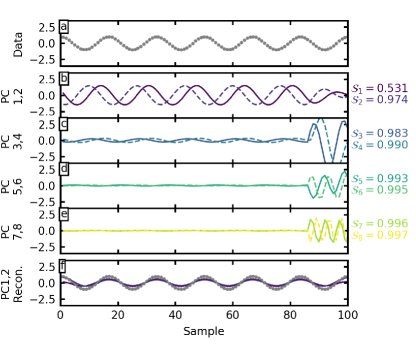
Figure 1: The cosine SSA example with $L=15$. Panel a shows the cosine data. Panels b-e show the first eight PCs, grouped into four pairs. Alongside each panel we list the normalised cumulative sum of the eigenvalues. Panel f shows the reconstruction of the first two PCs (coloured curves) and the sum of the first two PCs (grey) overlaid on the data.

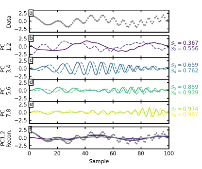
Figure 2: Same as Figure 1, but for the chirp SSA example.

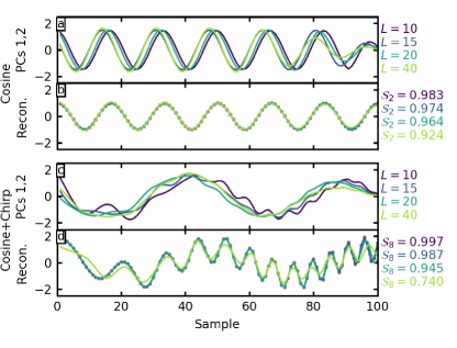
Figure 3: The effect of window sizes in the cosine example (panels a and b) and chirp (panels c and d). Panels a and c show the first two PCs for four different window lengths $L$. Panels b and d show the reconstruction from the first two PCs. The input data is shown in points. The normalised cumulative sum of the first two pp eigenfunctions is listed alongside.

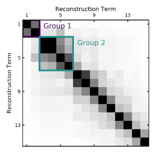
Figure 4: The distance matrix for the $L=15$ cosine + chirp example with low (high) distance represented as black (white). The top 2-by-2 block is the cosine- and sine-like PCs from the pure sinusoid (group 1; outlined in dark blue). The next 4-by-4 block contains the PCs that represent the chirp (group 2; outlined in green). These first 6 PCs contain 94% of the total variance. The k-means algorithm finds three groups, breaking the second 4-by-4 block into two 2-by-2 blocks. All PCs beyond the first 8 are insignificant; we show them here for completeness.

3.2 Separability

While the eigenpairs represent the best decomposition of the lag covariance matrix in the linear-least-squares sense, the eigenpair components are not guaranteed to represent unique dynamical features. In many cases, a single physical mechanism is spread into multiple components. We must group like components together to best elicit the mechanism. We will see an example of this in Section 5.1 when apply this method to our fiducial barred-galaxy simulation.

Our grouping procedure has two parts. First, we truncate the component series by only keeping eigenpairs that contribute significantly. Choosing how many eigenpairs or PCs to keep is a bit ambiguous especially for noisy time series. To be explicit, we define the maximum index $d$: $d=\max\{k:\ \lambda_{k}>\epsilon\}$, where $\epsilon$ is some threshold for the eigenvector to be in the null space. The run of $\log\lambda_{k}$ often has rapid drop off following by slowly decreasing plateau. A common heuristic truncates at the beginning of the plateau. This corresponds to the point of maximum curvature (often called the shoulder point) in the normalised cumulative sum $\mathcal{S}_{K^{\prime}}$ (eq. 18). This shoulder often corresponds to a cumulative normalised variance $\mathcal{S}_{K^{\prime}}>0.8$ and commonly closer to $\mathcal{S}_{K^{\prime}}\approx 0.95$. We have found it useful to characterise the truncation $\epsilon$ by the cumulative fraction of total variance at the truncation index.

Secondly, from the decomposition in equation (17), the grouping procedure partitions the set of indices $\{1,\ldots,d\}$ into $m$ disjoint subsets $I_{1},\ldots,I_{m}$. Define $\mathbf{C}_{I}=\sum_{k\in I}\mathbf{C_{k}}$. Equation (17) leads to the decomposition

$$\mathbf{C}=\mathbf{C}_{I_{1}}+\ldots+\mathbf{C}_{I_{m}}.$$ (22)

The procedure of choosing the sets $I_{1},\ldots,I_{m}$ is called eigenpair grouping. We will describe strategies for grouping below. If $m=d$ and $I_{k}=\{k\}$, $k=1,\ldots,d$, then the corresponding grouping is called elementary. The choice of several leading eigenpairs corresponds to the approximation of the time series in view of the well-known optimal property of the SVD. Grouping for our simple sinusoidal example, of course, is trivial: one pair of elementary matrices that contains all of the information about the signal.

The goal of grouping into sets $\{I_{k}\}$ is the separation of the time series into distinct dynamical components. Distinct time series components can be identified based on their similar temporal properties. For example, if the underlying dynamical signals are periodic, then the PCs will reflect that by producing sine- and cosine-like pairs with distinct frequencies. Thus, graphs of PCs or discrete Fourier transforms can help identify like components. For a real-world application, a quick visual examination of the $d$ PCs will suggest a group partition.

Very helpful information for separation is contained in the so-called $\mathbf{w}$-correlation matrix. This is the matrix consisting of weighted correlations between the reconstructed time series components. The weights reflects the number of entries of the time series terms into its trajectory matrix. Well separated components have small correlation whereas badly separated components have large correlation. Therefore, looking at the $\mathbf{w}$-correlation matrix one can find groups of correlated elementary reconstructed series and use this information to construct groups $\mathbf{C_{k}}$. The goal is to find groups such that uncorrelated reconstructed trajectories belong to different groups.

Mathematically, the elements $\mathbf{w}$-correlation matrix are related to the Euclidean-like matrix norm (also known as the Frobenius norm), defined as

$$||\mathbf{M}||_{F}=\sqrt{\sum_{i=1}^{n}\sum_{j=1}^{m}a_{ij}^{2}}$$ (23)

for an $n\times m$ matrix $\mathbf{M}$ (Golub & Loan, 1996). Specifically, let $\tilde{\mathbf{T}}^{k}$ be the reconstructed trajectory matrix defined in section 3.1.2. Define the normed trajectory matrix $\mathcal{T}^{k}=\tilde{\mathbf{T}}^{k}/||\tilde{\mathbf{T}}^{k}||_{F}$. Then, the elements of the $\mathbf{w}$-correlation matrix are

$$w^{1/2}_{\mu,\nu}=1-\frac{1}{2}||\mathcal{T}^{\mu}-\mathcal{T}^{\nu}||_{F}.$$ (24)

For insight, note that the same construction defines a metric distance

$$d_{\mu,\nu}=1-w^{1/2}_{\mu,\nu}=\frac{1}{2}||\mathcal{T}^{\mu}-\mathcal{T}^{\nu}||_{F}$$ (25)

between the two trajectory matrices. So the $\mathbf{w}$-correlation matrix describes the distance between reconstructed trajectory matrices. Thus, $w_{\mu,\nu}=0$ if the reconstructed series for PCs with indices $\mu$ and $\nu$ are orthogonal and $w_{\mu,\nu}=1$ if they are linearly dependent. The elements $d_{\mu,\nu}$ are a matrix which is the complement of the $\mathbf{w}$-correlation matrix which we will call the distance matrix.

From our experience, grouping is the trickiest and most sensitive part of the method; undergrouping will spread a single process into multiple features. For example, consider time series of coefficients from the basis EOFs from section 2 for some simulation. A single correlated dynamical signal may appear as several signals with very similar but slightly different principal components. For examples considered in section 5, we have grouped by examining the distance matrices to see which elements form obvious blocks. Often these blocks are obvious, and we provide an example in section 3.3. At the very least, for a strong nearly periodic perturbation such as a galaxy bar, nearly all significant eigenpairs come in phase pairs, corresponding to the cosine- and sine-like components of the oscillation. We then examine the reconstructions from eigenpairs by eye with insight from the distance matrices and regroup PCs whose reconstructions give similar time series. We have applied the k-means algorithm (Lloyd, 1982) to the set of normalised trajectory matrices $\{\mathcal{T}^{k}\}$ as an aid to grouping. This is fast and provides an automated first pass at grouping and the resulting closely corresponds to the visual impression of the distance matrices. For work in this paper, we will present distance matrices by rendering the elements $d_{\mu,\nu}$ rather than $w_{\mu,\nu}$ for interpretative consistency with our k-means classifier. (Kalantari & Hassani, 2019) advocated using hierarchical clustering methods which sensible but we have not explored this here. We will refer to groups defined by the distance between reconstructed trajectories for the eigenpairs. A number of authors have suggested Monte-Carlo hypothesis tests (Groth & Ghil, 2015) to provide objective criteria for the statistical significance of the oscillatory behaviour. This and other hypothesis testing will be explored as part of future work.

3.3 Some simple examples in depth

Consider a pedagogical data stream that is six cycles of the cosine function sampled at 100 evenly-spaced points. We then run the SSA machinery with window length $L=15$ to obtain PCs, eigenvalues, and reconstructions. Figure 1 shows the eigenvalues, PCs, and reconstructions for the pure sinusoid. Annotations report the normalised cumulative eigenvalues for the SSA analysis. As expected more than 97% of the power is the first two eigenpairs which represent the oscillation. The remaining eigenpairs are insignificant in the reconstruction. As a case in point, panels b-e show the first six PCs (paired into three groups). The first two represent the oscillation and the remaining PCs conspire to represent the truncation of the signal at the edge of the time series (e.g. PC3-PC8). Panel f shows the reconstruction of the time series for the first group (two PCs) and a comparison of the sum of PC1 and PC2 with the data. The sum of the reconstructions for PC1 and PC2 reproduces the data.

Now consider a time series that combines a low-frequency cosine with two cycles of the cosine function combined with a chirp function whose period increases linearly from three cycles at the beginning of the sample to none cycles at the end of the interval. As before, we create 100 evenly-spaced samples from the series. Figure 2 shows the data, PCs, and reconstruction for the $L=15$. In this case, the short window length mixes the signals together (e.g. PCs 1 and 2 do not form a clean phased pair that resembles either of the input signals).

The SSA algorithm will attempt to create a series of orthogonal functions that span the variation in a window length. For example, if we consider a series sampled from a simple rectangular (“top-hat”) function of some width $s<L$, the algorithm will construct orthogonal functions in the $L$-length interval whose lowest-order function is a triangle function, followed by antisymmetric, sine-like function and so on, each orthogonal to the next, in order to reproduce the input function. If the rectangle function has length $s=1$, the lag-covariance matrix will be the identity, and $L$ equal weight orthogonal functions will each be required to reproduce the series. So, the full scale of the temporal variation must be inside the window scale to be reconstructed. In addition, if the function is close to a continuous orthogonal function in the window, only fewer significant PCs will be needed for its representation. In this way, SSA has many analogous features to Fourier spectral analysis with the added feature of being adaptive to the time series itself.

Figure 3 explores the effect of window length $L$ on the first two PCs in the sinusoid and chirp examples. For the sinusoid example, we only show the first two PCs because the remaining PCs do not represent signal. Each period is sampled 16.7 points on average. We use window lengths that range from 10 to 40 samples, which illustrates the utility of M-SSA in cross-correlation of the lagged data. In all cases the fundamental frequency is well determined. For large window lengths, the PCs are distorted as the window hits the upper boundary of the time series. For example, the last several oscillations for $L=20,40$ are diminished in amplitude. Conversely, the $L=10$ does the best. Heuristically, $L$ needs to be large enough that a signal of interest varies over the window.

For the chirp case, a large window length can nicely separate the low-frequency from the high-frequency chirp, but the small $L$ values mix the signals together. As $L$ increases, the first two PCs approach the input cosine function and the remaining PCs represent the chirp. If the window length is too small to allow the lagged data replicates in the trajectory matrix to correlate over time, nothing will be learned from SSA. Indeed, for a lag of one, the covariance matrix is simply the variance in the signal and there is one PC: the time series itself. Similarly, if the window length is larger than half of the data length, the correlations at large lag will use very little of data for cross correlation and will yield nothing of significance. Therefore, the window length should be set to some value larger than the anticipated variation scale of the physical process and smaller than approximately half of the data length. Also note: a large window length leads to a large rank covariance matrix and large computational expense. So $L\to N/2$ should only be used if necessary.

Figure 4 is a graphical representation of the distance matrix defined by equation (25) that helps decide on PC grouping. Each element of the matrix indicates the degree of correlation between the reconstructed time series for each eigenpair. The maximum distance of 1 obtains for two orthogonal trajectories and the minimum distance of 0 obtains for two linearly dependent trajectories. Orthogonality or lack of any correlation is coded white and perfect correlation or linear dependency is coded as black. The most significant components will be in the upper left and the least significant components will be in the lower right. By examining the normalised sum of the eigenvalues or cumulative variance, we can restrict our attention to the first $K^{\prime}$ rows and columns of the correlation matrix corresponding to our desired significance level. Typically, this matrix divides itself up into blocks of correlated PCs. In some unusual cases, the rows and columns make need to be reordered to recover the natural blocking. By construction, the diagonal elements have distance 0. For our example, the first six eigenvalues represent 0.939 of the total variance, so we only consider the $6\times 6$ upper-left block. This block divides up cleanly into a $2\times 2$ that represents the cosine signal and a $4\times 4$ block that represents the chirp (cf. Figure 2).

For EOFs from section 2 describing an $N$-body simulation, reconstruction leads directly to density, potential and force diagnostics. We can use the $\tilde{a}_{m,i}^{I_{j}}$ to reconstruct the underlying potential or density fields in physical space using equations (7) or (8). We will provide examples in section 5.1.

4 Multichannel SSA (M-SSA)

4.1 SSA practice for multiple channels

We can now generalise the SSA to $M$ time series, here assume to be $M$ particular coefficients from equation (6): the set $\mathcal{M}=\{j_{1},\ldots\,j_{M}\}$. Following the previous section, denote each time series for the coefficient $a_{j}$ as:

$$A_{ji}=(a_{j,i},\ldots,a_{j,i+L-1})^{\top},\quad i=1\ldots,K.$$ (26)

where

$$\mathbf{A}_{j}=[A_{j1}:A_{j2}:\ldots:A_{jK}].$$ (27)

Then, the multichannel trajectory matrix $\mathbb{T}$ may be defined as

$$\mathbb{T}_{M}=\left[\mathbf{A}_{1},\mathbf{A}_{2},\ldots,\mathbf{A}_{M}\right].$$ (28)

The multichannel trajectory matrix has $KL$ columns with length $K=N-L-1$ (rows). The covariance matrix of this multichannel trajectory matrix is

$$\small\mathbf{C}_{M}=\frac{1}{K}\mathbb{T}_{M}^{\top}\cdot\mathbb{T}_{M}=\left(\begin{array}[]{lllll}\mathbf{C}_{1,1}&\mathbf{C}_{1,2}&\mathbf{C}_{1,3}&\ldots&\mathbf{C}_{1,M}\cr\mathbf{C}_{2,1}&\mathbf{C}_{2,2}&\mathbf{C}_{2,3}&\ldots&\mathbf{C}_{2,M}\cr\mathbf{C}_{3,1}&\mathbf{C}_{3,2}&\mathbf{C}_{3,3}&\ldots&\mathbf{C}_{3,M}\cr\vdots&\vdots&\vdots&\ddots&\vdots\cr\mathbf{C}_{M,1}&\mathbf{C}_{L,2}&\mathbf{C}_{L,3}&\ldots&\mathbf{C}_{M,M}\cr\end{array}\right)$$ (29)

where each submatrix is

$$\mathbf{C}_{j,k}=\frac{1}{K}\mathbf{A}_{j}^{\top}\cdot\mathbf{A}_{k}.$$ (30)

Each submatrix $\mathbf{C}_{j,k}$ has dimension $K\times K$ as in the one-dimensional SSA case. The multichannel covariance both auto-correlates individual series (as in SSA) and cross-correlates different time series simultaneously. Thus, the significance of temporal information that is common to multiple time series is reinforced.

The SVD step is the same as in the one-dimensional SSA. However, each eigenvector now has a block of length $K$, one block for each time series. Let us denote this as

$$\mathbf{E}^{k}=\left[\mathbf{E}^{k}_{1}:\mathbf{E}^{k}_{2}:\ldots:\mathbf{E}^{k}_{M}\right].$$

As for standard SSA, we obtain the PCs by projecting the trajectory matrix onto the new basis as follows:

$$P^{k}_{i}=\sum_{m=1}^{M}\sum_{j=1}^{L}a_{m,i+j-1}E^{k}_{m,j}.$$ (31)

The PCs are single orthogonal time series that represent a mixture of all the contributions from the original time series. It is again useful to define the normalised cumulative sum of the sorted $MK$ eigenvalues, where we will use the same notation as in equation (18), but with $M$ times more eigenvalues,

$$\mathcal{S}_{K^{\prime}}\equiv\frac{\sum_{k=1}^{K^{\prime}}\lambda_{k}}{\sum_{k=1}^{MK}\lambda_{k}},$$ (32)

where $K^{\prime}<MK$, to quantify the relative importance of eigenvectors across channels.

Finally, the last step of the process reconstructs the original time series of index $m\in[1,\ldots,M]$ from the PCs as follows:

$$\small\tilde{a}^{k}_{m,j}=\begin{cases}\displaystyle\frac{1}{j}\sum_{n=1}^{j}P^{k}_{n-j+1}E^{k}_{m,n}&\mbox{if}\ 1\leq j<L-1,\\ \displaystyle\frac{1}{L}\sum_{n=1}^{L}P^{k}_{n-j+1}E^{k}_{m,n}&\mbox{if}\ L\leq j\leq N-L+1\\ \displaystyle\frac{1}{N-j+1}\sum_{n=1-N+M}^{N}P^{k}_{n-j+1}E^{k}_{m}&\mbox{if}\ N-L+2\leq j\leq N.\\ \end{cases}$$ (33)

If we sum up all of the individual PCs, no information is lost; that is:

$$a_{m,i}\rightarrow\sum_{k=1}^{d}\tilde{a}^{k}_{m,i}$$ (34)

As described in section 3.2, we often want to sum up the reconstructions for specific groupings:

$$\tilde{a}_{m,i}^{I_{j}}=\sum_{k\in I_{j}}\tilde{a}^{k}_{m,i}$$ (35)

which gives us the parts of of each coefficient $a_{l}(t)$ that correspond to each dynamical component $I_{j}$.

Overall, the M-SSA steps exactly parallel the SSA steps but with more bookkeeping. M-SSA rather than the simpler SSA is necessary for our application to coefficient time series of biorthogonal EOFs. For any particular application in galaxy dynamics, the evolution gravitational field will correlate several basis functions. So one would have incomplete signal if one performed $M$ individual SSAs rather than a single M-SSA. However, the more time series we use, the larger the risk of mixing power between components owing to noise or unsteady behaviour. In several of our examples below, we use both EOFs from the gravitational field and functional representations of the velocity fields. This mixing is most like amplified when series with different units are combined. To combat this, we detrend each time series by subtracting the mean and normalise the time series by the variance. When combining multiple types of data, one may weight one type relative to the other. We have not done this in our work in section 5 but it remains an option.

We may continue to group eigenpairs using the $\mathbf{w}$-correlation or the using k-means clustering and the Frobenius norm. For the applications targeted in this paper, the multiple channels represent spatial features and kinematic signals induced gravitationally by the same mass distribution, so they will be naturally coupled. To aid in grouping, we apply the methods from section 3.2 to each reconstructed channel separately and look for similarities in the block or group structure as a whole. Also, we may consider the $\mathbf{w}$-correlation matrix and k-means classification using the distance defined from the matrix norm of the reconstructed the multichannel trajectory matrix $\tilde{\mathbb{T}}$ for each elementary matrix:

$$\tilde{\mathbb{T}}_{M}^{k}=\left[\mathcal{T}_{1}^{k},\mathcal{T}_{2}^{k},\ldots,\mathcal{T}_{M}^{k}\right].$$ (36)

where each of the $\mathcal{T}^{k}_{j}$ are reconstructed series for the $j^{th}$ channel and the $k^{th}$ eigenpair and

$$||\tilde{\mathbb{T}}_{M}^{k}||_{F}=\sqrt{\sum_{l=1}^{M}\sum_{i=1}^{n}\sum_{j=1}^{m}(\mathcal{T}^{k}_{lij})^{2}.}$$ (37)

This is the naturally generalisation of the development in section 3.2. Although we have not seen this described elsewhere, is seems like a natural extension of the $\mathbf{w}$-correlation concept and is useful in practice. Geometrically, this extended metric is equivalent to considering vectors the space defined by the concatenation of time series for all channels. So this multichannel $\mathbf{w}$-correlation describes total distance between the reconstructed series for each PC for all channels together. If all channels mutually take part in a signal of interest, then combined distance will help discriminate groups by providing more evidence than any channel individually. Conversely, independent channels will form disjoint subspaces and therefore not affect the distance between group members. Noisy channels, however, could degrade separation of groups, so it is up to the practitioner to choose channels wisely. Also, it would be possible to weight the contribution to the total distance by channel based on some prior assignment of channel importance, but this has not been explored here.

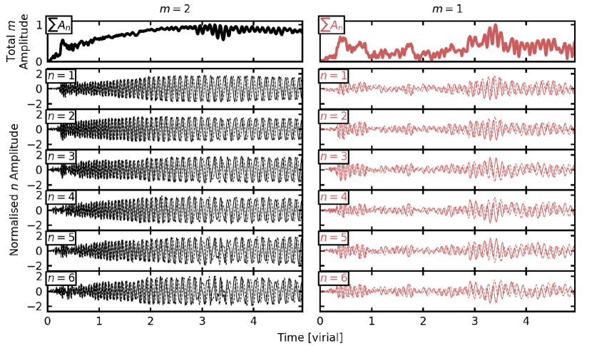
Figure 5: Coefficients of the basis function expansions for harmonic orders $m=2$ (right) and $m=1$ (left) of the fiducial bar simulation. The upper row shows the total modulus for the harmonic orders. The remaining panels show the first $n=6$ radial orders in cosine (solid) and sine (dashed) series.

4.2 Other applications of M-SSA

While our main goal in this paper is the discovery of dynamical mechanism, M-SSA has a number of other applications to simulations. The most obvious one is data compression. In many cases, a small number of eigenpairs relative to the total number $MK$ have the lion’s share of the variance; that is: $S_{K^{\prime}}\approx 1$ for $K^{\prime}\ll MK$ in the notation of equation (32). Therefore, we can reconstruct most of the dynamics with a small number of eigenpairs. This reduces the important information in a simulation to very small manageable summary. For example, the dominant PCs or their reconstructions might provide a framework for classifying the dynamical patterns in a suite of simulations using some distance metric (e.g. the Frobenius norm).

Similarly, we can consider diagnostics of per channel contributions. Although, we have not seen M-SSA used this way, equations (33) and (35) lend themselves to an estimate of the fraction of each coefficient in any particular eigenpair or group. Specifically, let us measure the contribution of the $k$th eigenpair to the $j$th coefficient by:

$$f^{k}_{j}\equiv\frac{||\tilde{\mathbf{a}}^{k}_{j}||_{F}}{||\tilde{\mathbf{a}}_{j}||_{F}},$$ (38)

where the Frobenius norm $||\cdot||_{F}$ described in section 3.2. By definition $0<f^{k}_{j}<1$ and $\sum_{k}f^{k}_{j}=1$. Thus, $f^{k}_{j}$ tells us the fraction of time series $j$ that is in PC $k$. This tells us whether the particular EOF $j$ plays a role in generating the dynamical mechanism. Alternatively, we may compute

$$g^{k}_{j}\equiv\frac{||\tilde{\mathbf{a}}^{k}_{j}||_{F}}{\sum_{j=1}^{M}|\tilde{|\mathbf{a}}^{k}_{j}||_{F}},$$ (39)

which is the fraction of PC in series $j$. Thus, the histogram $g^{k}_{j}$ reflects the partitioning of power in the PC $k$ into the input coefficient channels $j$. So, we can think of this representation as a single matrix, normed on rows in the case of $f$ and normed on columns in the case of $g$. In both cases, the norm over the time series may be restricted to some window smaller than the total time series. We have not used this in section 5, but just like compression, it may be useful in the future for culling degrees of freedom that are informative from those that are noise-dominated.

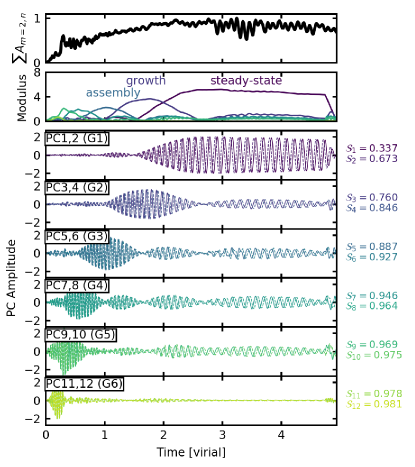
Figure 6: Illustration of M-SSA decomposing the bar simulation into physically-informative PCs. The upper row shows the sum of the $m=2$ moduli across all $n$ orders. The second row shows the modulus of each eigenpair of PCs. The phases of bar evolution from (Petersen, Weinberg & Katz, 2019a) are labelled. The remaining panels show the PC pairs, with cosine-like terms shown as solid lines and sine-like terms shown as dashed lines.

5 Simulation examples

We feature the fiducial model from Petersen, Weinberg & Katz (2019a, b, c, hereafter Paper 1, Paper 2, and Paper3, respectively). This model was chosen to be representative of a current-time Milky-Way-like galaxy. These papers provided a detailed dynamical analysis of the possibly interacting channels of secular evolution using orbit analysis, torques, and harmonic analysis. Specifically, we found evidence for three phases in evolution with unique harmonic signatures. We recovered known results, such as bar slowdown owing to angular momentum transfer, and identified a new steady-state equilibrium configuration and harmonic interaction resulting in harmonic mode locking.

Because some of these dynamical features will be familiar to many dynamicists, they provide a pedagogical benchmark for M-SSA. In the first example (section 5.1), we will show that the simplest application of M-SSA immediately identifies the bar, its secular growth, and its subsequent pattern-speed decay as a function of time. M-SSA effectively compresses the dynamical simulation by many orders of magnitude into a low-dimensional summary of the key dynamical feature: the evolution of the bar as a function of time. In the second example (section 5.2), we apply M-SSA to the both the dipole and quadrupole harmonic disc expansion coefficients simultaneously. In addition to the $m=1$ bar coupling reported in Petersen, Weinberg & Katz (2019b), M-SSA reveals that the bar drives power into the natural $m=1$ mode of the galaxy described in Weinberg (1994). Finally in sections 5.3 and 5.4, we explore an extension of basis-function analysis that combined both our biorthogonal basis functions and a cylindrical expansion of the velocity fields. In the first velocity example, we recover the bar-induced velocities; in the second velocity example, we quantify the velocity signature during a period of horizontal-vertical coupling.

5.1 Simple bar analysis from fiducial simulation

This section is a direct application of the development in section 4 of our three-dimensional cylindrical disc expansion described in section 2 (see the appendix of Paper 1 for more detail). For a quick review, Paper 1 presents a pair of simulations, one with a cuspy halo and one with a cored halo that are designed to rapidly form bars. In the examples considered below, we will study the cuspy halo from Paper 1 and refer to it has the fiducial simulation. An exploratory analysis for an already well-studied simulation makes for a straightforward identification of dynamical features in our new method.

The bar dominates the dynamics of the fiducial simulation. The strongest dynamical feature of the barred galaxy density and potential is a rotating quadrupole. Therefore, a study of the temporal and spatial features in the $m=2$ harmonic subspace by M-SSA is a good first test. Our simulation records the coefficient time series for steps of $h=0.002$ (or approximately every 4 million years in Milky Way units). We excerpt the first 12 coefficient time series for the $m=2$ harmonic of the cylindrical basis described in section 2. These become the $\hat{a}_{j},j=0,\ldots\,11$, the particle-estimated versions of $a_{j}$ in equations (26)–(29). The run of the $m=2$ coefficients is shown in the left panels of Figure 5. The slowing bar pattern speed and time-dependent amplitude envelope are shared by all the series for fixed $m$. Other distinct dynamical features are not obvious from this figure.

We now perform the M-SSA on these series. Computational efficiency motivates pruning the time series and carefully choosing the window length, $L$ in equations (26) and (27). First, and especially for the bar-driven dynamics, we may subsample the time series by striding. For our case, we use a stride of 2, every other time step. Second, we set the window size to $L=200$; this implies that we are sensitive to intervals of at most $\Delta T=0.4$ time units (or approximately 1 Gyr in Milky Way time units). We vary $L$ to check our sensitivity to this choice. Increasing $L$ by a factor of two or four does not substantively change the dominant PCs. Our final matrix has rank $2400\times 2400$. Finally, the PCs corresponding to the eigenpairs, their eigenvalues, and an inspection of reconstruction corresponding to each, M-SSA provides an efficient representation of the dynamics.

For our fiducial bar simulation, approximately 93% of the total power is represented in the first six eigenpairs (out of 2400). Both a by-eye examination of the distance matrix $d_{\mu,\nu}$ for the coefficients that make up the bar using equation (36) and the k-means analysis described in sections 3.2 and 4.1 suggests that the first six clusters are pairs of eigenpairs, which we label as groups 1-6. As described in sections 3–4, a periodic signal results in pairs of eigenpairs with similar eigenvalues. These are analogous to the sine and cosine terms required to represent a periodic signal in a Fourier analysis. SSA does not force any particular PC to have a constant frequency, but an approximate periodicity will result in pairs nonetheless. The dynamics driven by bar formation and evolution is, of course, driven by the strong quasi-periodic non-axisymmetric bar potential, so the dominant eigenpairs come in cosine- and sine-like pairs. The first six PC groups are plotted in Figure 6. The lowest-order group, which dominates the gravitational power, represents the bar after its formation and growth phases (see Petersen, Weinberg & Katz 2019a for more discussion of bar evolution phases). The magnitude of any particular pattern identified by M-SSA will depend on both the strength of the excitation at peak and the duration of the excitation in the time series. In this time series, the simulation spends nearly half of its total time in slow evolution. Panel b of Figure 6 combines the cosine- and sine-like components into a modulus. This panel succinctly summarises the contribution of each PC to the bar feature as a function of time. Also note from Figure 6 that the bar rotation period continues to decrease throughout the evolution. Unlike a traditional Fourier analysis, M-SSA identifies coherent, persistent dynamical patterns which may include multiple and evolution frequencies.

While the first three groups represent 93% of the total variance in $m=2$, there are many other lower-amplitude but significant features revealed by M-SSA. PC5 + PC6 depict early development of the $m=2$ disturbance that will lead to bar formation. PC7 + PC8, in particular, depict transient spiral-arm activity. These are strongest during bar formation but reoccur at different patterns throughout the simulation. The pattern speed of the arms is different than those of the bar, as expected.

Figure 8 illustrates the summary nature of M-SSA by demonstrating a density reconstruction with a small number of $m=2$ coefficient series (see Figure 5) and time-domain PCs. We purposely choose $T=2$ which is during the transition from the secular growth phase to the steady-state phase. In addition, we include the $m=0$ coefficients in the reconstruction of the bar density to give a better sense of the true density rather than the density difference. We have investigated a joint $m=0$ and $m=2$ M-SSA computation and find that the $m=0$ coefficients are primarily captured in a single PC pair. This is expected: changes in the $m=0$ field are on a secular time scale, which is much longer than the bar dynamical time. The upper row in Figure 8 shows that the bar is close to converged after the first four basis functions are coadded. The ‘A1-6’ panel is the final bar density reconstruction. The ‘dimples’ perpendicular to the bar are filled in by higher order harmonics (principally $m=4$) that are not included in this reconstruction. The lower row in Figure 8 is the reconstruction of the bar density from the PCs (see Figure 6). From left-to-right, we add successively more PCs to the reconstruction. Despite selecting a time when the PCs suggest that the bar is in a dynamical transition (between growth and steady-state), the PCs are able to reconstruct the primary features of the bar density with only two PC pairs. If we chose a time in the centre of a phase, the bar would be reconstructed with a single PC pair. This demonstrates the compressive power of M-SSA to reconstruct the bar: two PC pairs are able to accurately represent the bar, even during a dynamical transition, while the coefficients require the full $n\leq 6$ radial functions to represent the bar density.

In summary, the M-SSA approach to dynamical analysis of our fiducial bar simulation in time automatically identified many of the key results from Paper 1. Moreover, subdominant but apparently statistically significant features such as spiral arm activity can be located in time quantified in amplitude. None of these features could be inferred from examining Figure 5 alone, although the information is in these series. That said, M-SSA does not uniquely identify distinct dynamical components. For example, the bar itself is spread over multiple PCs in the analysis here.

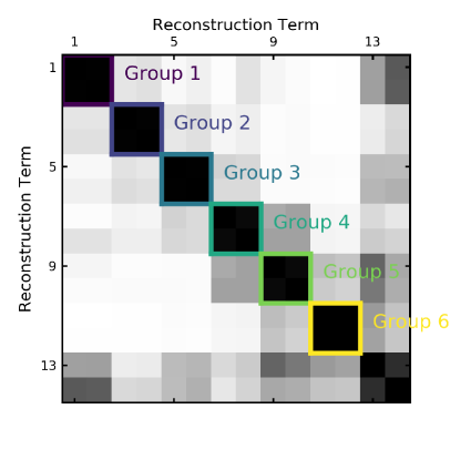
Figure 7: The distance matrix for the $m=2$ case with low (high) distance represented as black (white). The first six groups (all pairs of PCs) are labelled..

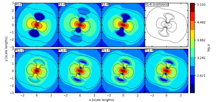
Figure 8: Demonstration of information compression for the $m=2$ example at $T=2.0$ using M-SSA. Upper: the reconstruction of the bar density from the $m=2$ coefficients (see 5) as filled contours for radial basis functions m through n, denoted as Am–n in each panel. Lower: we show the reconstruction of the bar using PCs, adding successively more PCs, denoted similarly (see PCs in Fig. 6). In all panels, we apply the $m=0$ coefficients from the simulation to approximate total density rather than the relative density from only the $m=2$ coefficients. The upper right panel shows only the empty contours from the reconstruction of the bar density from $n\leq 6$, which we then overlay on each other panel for comparison.

5.2 Combined $m=1$ and $m=2$ analysis from fiducial simulation

Paper 2 describes an $m=1$ and $m=2$ non-linear interaction that results when the previously independent pattern speeds become commensurate. Here, we take a temporally global look at the interaction using M-SSA. Specifically, we choose the first six radial components from each of $m=1$ and $m=2$ for $M=24$ total time series in equations (26)–(29). The run of the $m=1$ coefficients is shown in the right panels of Figure 5. The PCs from the $m=1+m=2$ analysis are shown in Figure 9. We grouped the individual eigenpairs by similarity of their PCs and blocks in the distance matrix (Figure 10; section 3.2). For all but one group, these were adjacent pairs of PCs. One particular group had three similar eigenpairs.

Overall, the $m=1$ and $m=2$ coefficient series are mixed into multiple PCs. The dominance of both harmonics vary from time to time in individual PCs but tends to toward a stable split during periods of similar evolution, i.e. the evolutionary phases described in Paper 1. For example, after the bar forms, PCs1–2 are dominated by $m=1$ while PCs3–6 are dominated by bar-like $m=2$ similar to the previous subsection. During the pre-formation, formation and growth phases of the bar evolution, both $m=1$ and $m=2$ coexist. The density evolution of each harmonic seems distinct within each phase. Overall, PCs1–10 describe a joint $m=1$ and $m=2$ modulated interaction with an coherent pattern speed. The block consisting of the first four PCs describe the late-time resonant interaction (Group 1) and the second block (PC5–10) describes an early-time burst of interaction that fades after bar growth (Group 2). As the $m=1$ and $m=2$ patterns become resonant at $T\approx 3$, PC1–4 dominate and the bar appears to slosh from side to side. At the same time, PC11–12 appears with an $m=1$ signature with a very slow retrograde pattern (Group 3). This block is significant with respect to the first two blocks with 4% of the total power. The two-dimensional density profiles for Groups 1 and 3 are shown in Figure 11.

While the patterns in the primary PCs are clear by eye in a density animation from the fiducial simulation, detection of the retrograde pattern required this M-SSA analysis! We did not see this in the animation directly. The existence of weakly damped $m=1$ modes in spherical systems was reported in Weinberg (1994). For a spherical symmetric system, this mode comes in prograde and retrograde pairs. Subsequent work showed that in the presence of a disc, the joint halo and disc mode splits into a very weakly damped retrograde mode and less weakly damped prograde mode. So, in this context, the result found by M-SSA is not a complete surprise. But it was unanticipated and illustrates the power of M-SSA to find dynamical correlations that are not evident by visual inspection.

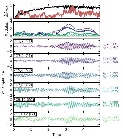
Figure 9: Illustration of M-SSA decomposing the combined $m=1$ and $m=2$ coefficients from bar simulation into physically-informative PCs. The upper row shows the sums of the $m=1$ and $m=2$ moduli across all $n$ radial orders. The second row shows the modulus of each eigenpair of PCs. The remaining panels show the PC pairs, with cosine-like terms shown as solid lines and sine-like terms shown as dashed lines. The group association for each PC pair is listed in the upper left corner of the panel.

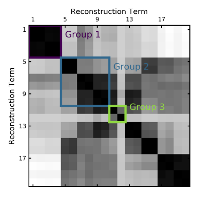
Figure 10: The distance matrix for the $m=1+m=2$ case with low (high) distance represented as black (white). The first three groups are outlined and labeled.

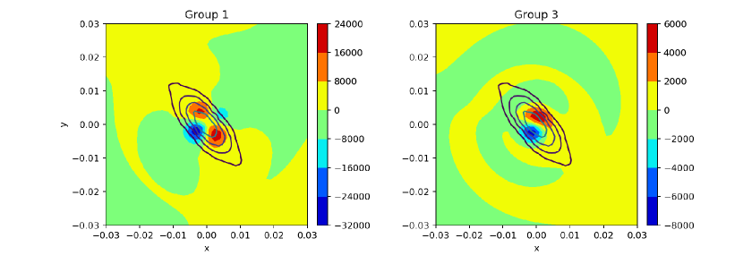
Figure 11: The reconstructed surface density profiles based on the combined $m=1$ and $m=2$ coefficients for the two eigenpair groups described in Figure 9. The first group shows the quadrupole modulated by a dipole; an animation of surface density for the full simulation shows the bar to sloshing from side to side. The left-hand plot shows this as higher intensity in direction of negative x, positive y. The second group shows a retrograde $m=1$ with the very slow oscillation frequency (Group 3). Logarithmically spaced contours in surface density is overlaid in the lower row for reference.

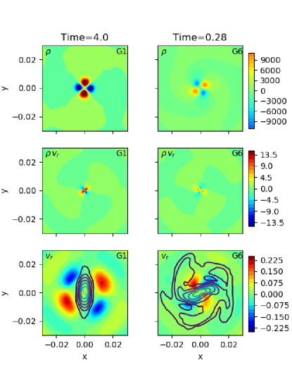
Figure 12: The density (top row), density times velocity (middle row) and velocity field (lower row) for two PC groups (columns) in the fiducial bar simulation. Each column shows the PC group close to its time of peak amplitude (labeled at the top of each column). The initial scale length of the disc is 0.01 virial units and the peak rotation curve is $\approx 1.4$ in virial units. The peak velocity features are 40 km/s when scaled to the Milky Way. Logarithmically spaced contours in surface density is overlaid in the lower row for reference.

5.3 Combined spatial and kinematic signatures from fiducial

Although the phase space for any physical system of interest is a complete description, the history of the density and gravitational field alone is incomplete; we need the flow or momentum information for a complete description. For this reason, the combination of density and kinematic data together powerfully constrains dynamical hypotheses while density alone does not. In addition, density and kinematics are readily compared with observational data. Therefore, a methodology that uses simulations to develop discriminating statistical tests is desirable, and M-SSA offers this possibility. As in sections 5.1–5.2, our strategy is a join of multiple time series of coefficients describing fields of interest. There are two obvious choices for the join: combining a set of biorthogonal coefficients from expansions in the form of equations (6)–(8) combined with radially local orthogonal coefficients or radially global orthogonal coefficients representing the velocity fields. Locally orthogonal coefficients include the standard Fourier set at fixed cylindrical radius $R$, e.g.

$$c_{mj}(R) = \frac{R}{2\pi}\int_{0}^{2\pi}d\phi\,\cos(m\phi)\Sigma(R,\phi)v_{j},$$ (40)

$$s_{mj}(R) = \frac{R}{2\pi}\int_{0}^{2\pi}d\phi\,\cos(m\phi)\Sigma(R,\phi)v_{j},$$ (41)

where $v_{j}$ is some particular component of the velocity in cylindrical coordinates ($v_{R},v_{\phi},v_{z}$). These functions are orthogonal for all $m$ at fixed radius $R$. One might use vector spherical harmonics (e.g. Hill, 1954) to accomplish the same decomposition for spherically extended systems. We choose to expand the product of the surface density and velocity to match the natural weighting from an N-body simulation. Evaluated at the positions of individual particles, $\Sigma(R,\phi)=\sum_{i=1}^{N}m_{i}\delta(R_{i})\delta(\phi_{i})/R_{i}$, equations (40)–(41) become:

$$\hat{c}_{mj}(R) = \frac{1}{2\pi}\sum_{i}^{N}\cos(m\phi_{i})m_{i}v_{ij},$$ (42)

$$\hat{s}_{mj}(R) = \frac{1}{2\pi}\sum_{i}^{N}\sin(m\phi_{i})m_{i}v_{ij}.$$ (43)

We will call this a ring expansion for a two-dimensional cylindrical case and a shell expansion for a three-dimensional spherical case.

This approach works, but strong non-axisymmetric disturbances produce correlated kinematic signatures over a range in radii. In this situation, we find that ring and shell expansions are noisy and inefficient; it spreads the correlated signal over a large number of series. An examination of the flow field in a bar immediately identifies a problem: the $x_{1}$ bar orbits move through the individual rings over very narrow ranges of azimuth. Therefore the ring average of $v_{r}$ or $v_{t}$ is very small. In this way, rings dilute the non-axisymmetric flow. For the fiducial bar model considered in the sections above, the ring analysis only resulted in strong signal during times of strong transient disturbance that occur between evolutionary phases.

To circumvent this bias, we propose using a globally distributed basis in radius. The natural choice for a finite radial range is cylindrical Bessel functions, $J_{n}(\alpha_{mj}R)$, for discs and spherical Bessel functions, $j_{n}(\alpha_{lj}R)$, for spherical distributions, where the constants $\alpha$ are chosen according the standard orthogonality conditions (Watson, 1966). However, it is better to choose a basis whose lowest-order function resembles the disc density. To this end we define a Laguerre basis with functions defined by

$$G_{n}(R;a)=\gamma_{n}(a)e^{-R/a}L_{n}^{\{1\}}(2R/a)$$ (44)

where $g_{n}=[a^{2}(n+1)]^{-1/2}$ is the normalisation and $L_{n}^{\{\alpha\}}(x)$ is the generalised Laguerre polynomial (e.g. Abramowitz & Stegun, 1964). These functions obey the scalar product:

$$\left(G_{j},G_{k}\right)=\int dR\,RG_{j}(R;a)G_{k}(R;a)=\delta_{jk}.$$ (45)

Then, the expansion coefficients for any field component $v(\mathbf{x})$ may be written as:

$$C_{mj}[v(\mathbf{x})] = n_{m}\int_{0}^{\infty}dRRG_{j}(R;a)\int_{0}^{2\pi}\cos(m\phi)\rho(\mathbf{x})v(\mathbf{x}),$$

$$S_{mj}[v(\mathbf{x})] = n_{m}\int_{0}^{\infty}dRRG_{j}(R;a)\int_{0}^{2\pi}\sin(m\phi)\rho(\mathbf{x})v(\mathbf{x}),$$

where $n_{m}=\left[(\delta_{m0}+1)\pi/2\right]^{-1/2}$ is the normalisation for trigonometric functions and $v(\mathbf{x})$ are one of the cylindrical velocity components $v_{r},v_{t},v_{z}$. Analogous to the rings, the particle estimators for equations (LABEL:eq:cosBv) and (LABEL:eq:sinBv) are:

$$\hat{C}_{mj}[v(\mathbf{x})] = n_{m}\sum_{i=1}^{N}m_{i}G_{j}(R_{i};a)\cos(m\phi_{i})v(\mathbf{x}_{i}),$$ (48)

$$\hat{S}_{mj}[(v(\mathbf{x})] = n_{m}\sum_{i=1}^{N}m_{i}G_{j}(R_{i};a)\sin(m\phi_{i})v(\mathbf{x}_{i}).$$ (49)

These coefficients represent the product of the density $\rho(\mathbf{x})$ and field quantity $v(\mathbf{x})$. We represent the product $\rho v$ rather than field alone $v(\mathbf{x})$ to facilitate evaluation of the coefficients $C_{mj},S_{mj}$ from the particle set. In many cases, we would really like $v(\mathbf{x})$ rather than $\rho v$, and this can be evaluated by dividing by an independent estimate of $\rho$ (e.g. a binned surface density from the particles).

As an example, we used the $m=2$ time series from section 5.1 with 8 radial orthogonal functions ($n\leq 4$ in Figure 5) and the Laguerre expansion with 8 functions. There are no obvious new features in the PCs as a result of adding the kinematic time series. This is confirmed by computing the M-SSA analysis for the 8 Laguerre coefficient series alone and recovering nearly the same PCs up to 95% of the total variance. However, we do see that the density and kinematic data together better discriminate the bar-specific and spiral-arm specific patterns. We plot the density, the density times radial velocity, and radial velocity reconstruction for each PC group near its peak amplitude in Figure 12. The velocity fields are computed from the reconstruction of $\rho(\mathbf{x})v_{r}(\mathbf{x})$ divided by the binned surface density.

The bar is present at the time sampled for groups G1-G5. Groups G1-G5 are very similar in morphology but peak at different times as described in section 5.1; therefore, we only show the reconstruction from G1 in Figure 12. The first group (G1) is the first pair of PCs and represents the bar feature at late times in its steady-state phase. Since trapped bar have a prograde circulation with odd parity relative the bar major axis, we expect the line of nodes for $\rho v_{r}$ to align with the bar density $\rho$; this is clearly seen for G1 (Figure 12). The quantity $\rho(\mathbf{x})v_{r}(\mathbf{x})$ depends both on the density of the disc and its velocity field. So each of the three quantities illustrates an aspect of the three interrelated quantities. For example, the most obvious kinematic flow features follow the same trend as orbits inside the bar but large radius near the maximum extent of the trapped bar. These regions have very low orbit occupation, however.

The left-hand column in Figure 12 shows G6 which represents a strong $m=2$ spiral feature before the formation of the bar; this spiral is prominent in the kinematic pattern. PCs in this group represent spiral arm activity at early times (cf. Figure 6), before and during bar formation, and at later times at lower amplitude with pattern speeds that are lower than that of the bar. This suggests that the joint density/potential and kinematic expansion may be more powerful in some cases than density/potential expansion alone. In this case, however, either the density and kinematic fields determine the PCs on their own.

We have repeated this analysis for $\rho v_{t}$ and reproduced the expected phase-shift in the phase with respect to the density line of nodes. This might be expected since $v_{r}$ and $v_{t}$ are correlated for the $x_{1}$ orbits that dominate the bar structure. Similarly, the analysis includes $v_{z}$. Our disc EOFs are either vertically symmetric or antisymmetric with respect to the vertical midplane (see section 2 and Petersen, Weinberg & Katz 2019a). This allows immediate diagnosis of vertical distortions. To check for changing vertical structure, we performed the analysis with the vertically anti-symmetric EOFs together with Laguerre velocity coefficients: power in anti-symmetric EOFs indicates changing vertical structure. Our fiducial simulation does not display any significant vertical features in the bar and M-SSA recovers this result.

5.4 Application to vertical coupling

For a disc of constant surface density, the vertical orbital frequency decreases with increasing scale height. Depending on the disc and halo models, the bar pattern speed may approach commensurability with the vertical orbital frequency as the bar slows. The resulting resonant coupling exchanges horizontal and vertical action (e.g. Sridhar & Touma, 1996; Quillen, 2007) results in an increase of vertical extent for resonant orbits. If the resonant orbits are in phase, the observed signal is a bobbing of the orbits above and below the plane in phase with bar pattern. While the mechanism appears to be more closely related to the levitation described by Sridhar & Touma (1996), our goal here is to illustrate the use of vertical symmetry in both spatial density and velocities to detect and quantify the vertical feature. This mechanism called alternatively called ‘bending’ or ‘buckling’ in the literature (Raha et al., 1991; Debattista et al., 2006; Sellwood & Gerhard, 2020). While asymmetries in the bar with respect the disc mid plane produces a transient vertical asymmetry in some cases, this appears to damp in time (see Petersen & Weinberg 2020).

Our example simulation is very similar to the fiducial model discussed throughout this paper but with a scale height that is two times larger. The square root of the quadrupole power or total amplitude is illustrated in Figure 13 (top). The horizontal-vertical resonance begins to affect the disk at $T\approx 2$ with a rapid rise in vertical power beginning at $T\approx 2.6$ and culminating in a readjustment of the bar support at $T\approx 2.9$. Some additional vertical activity persists and damps away between $T=4$ and 5.

To describe the vertical evolution using M-SSA, we find the principal components for the join of the first 8 Laguerre coefficients from equations (48) and (49) with $v=v_{z}$ and one of (1) the first 6 vertically symmetric BFE coefficients; (2) the first 6 vertically anti-symmetric coefficients; and (3) no BFE coefficients. Let us now compare the results for each of these three cases. The first three PC groups for each analysis, representing more that 50% of the power in each case are shown in Figure 13 (lower panels). Recall from section 3 that the PCs represent a mixture of all time series.

In Case 1, Group 1 represents the long-term evolution the bar after the vertical evolution without any vertical kinematic correlation. Group 2 picks out a combination of in-plane changes and vertical motion associated with the horizontal-vertical resonance that begins at $T\approx 2$ and rapid grows in amplitude $T\approx 2.6$ to $T\approx 2.9$. Group 3 represents the readjustment of the bar that is correlated with decay of the kinematic vertical power. Case 2 tells a similar story. However, the now only the correlations between anti-symmetric vertical density and kinematics are represented. The dominant Group 1 describes the initial coupling between the bar and vertical motion. Groups 2 and 3 represent the longer-term decaying vertical transient. The PCs describing the long-term bar evolution is absent. This implies that the vertical coupling has finite duration. A study of this dynamics suggests that the primary vertical interaction occurs when the 2:1 azimuthal to vertical frequency resonance reaches the end of the bar. This is followed by some transient trapping. However, Case 3 differs significantly from the first two, suggesting that the kinematics alone is insufficient to uniquely determine the temporal patterns between the spatial and kinematic variation. In particular, Case 3 (bottom panel in Fig. 13) puts emphasis on the vertical motion resulting from the resonance for all three PC groups. Higher-order PCs describe the noisy features seen in Figure 13 (top) for $T\lesssim 1.5$. The oscillation in Figure 13 (top) corresponds precisely to the bar pattern; M-SSA finds no independent pattern speed suggesting that there is no separate mode governing bending.

The differences in the temporal structure revealed by the three M-SSA case studies illustrate the influence of series selection. We find that both vertically symmetric and antisymmetric EOFs will detect the vertical interaction, but will highlight different facets of the dynamics. Case 1 teaches us that in-plane dynamics dominates the long-term bar evolution. The analysis reveals lower-amplitude evidence of the horizontal-vertical coupling at the same frequencies as the bar, suggesting that the interaction is strongly bar driven. Case 2 focuses on the vertical structure by correlating the antisymmetric density and potential excitation with vertical streaming. This reveals several stages in the interaction: an initial resonance which couples the planar angular momentum to vertical degrees of freedom followed by a slowly decaying transient in vertical asymmetry. Case 3 considers vertical velocity streaming only; this suggests that significant vertical streaming dominates only between the onset of the resonance but before a structural response. One must carefully select series that contain the relevant information for the dynamical question at hand.

Figure 14 compares the reconstruction of the velocity signal, $\rho(\mathbf{x})v_{z}(\mathbf{x})$ and $v_{z}(\mathbf{x})$, with the vertically anti-symmetric component of disc density $\rho(\mathbf{x})$ from Case 2. Large positive or large negative values of $\rho(\mathbf{x})v_{z}(\mathbf{x})$ (middle panel) and $v_{z}(\mathbf{x})$ (bottom panel) indicate regions dominated by significant upward and downward mean orbital motions, respectively. Consider a bar-supporting orbit in the frame of the bar rotation. Figure 14 tells us that a representative orbit moves upwards as it moves from apocentre to pericentre and downwards from pericentre to apocentre. Figuratively, the orbits follow a saddle-shaped warped surface whose line of nodes aligns with the bar. Comparing all three panels, we see that the vertical $m=2$ feature is characterised by the inner bar moving in the opposite direction vertically as the outer bar. The velocity streaming is dominated by vertical motions in the outer bar. The top panel shows a cut through the $x$–$z$ plane. The multiple sign-changes in the vertical density arises from the in-phase oscillation of orbits near the horizontal–vertical resonance at different radii owing to interaction with the existing transient structure.

M-SSA reveals that the bar is not bending dynamically but stays bent after the initial vertical coupling, slowly settling back to the disc mid plane in time. This pattern is preserved for many bar rotations. By symmetry, orbits that downwards as they move from apocentre to pericentre and upwards from pericentre to apocentre should be equally likely. This suggests that some transient or phase dependence is responsible for the sign of the vertical bobbing. Indeed, the decay of the anti-symmetric power seems to correspond to a homogenisation of these two perpendicular phases. After mixing, the bar has the characteristic boxy or peanut shape. We will use these tools to describe the dynamics of these vertical features in a later paper.

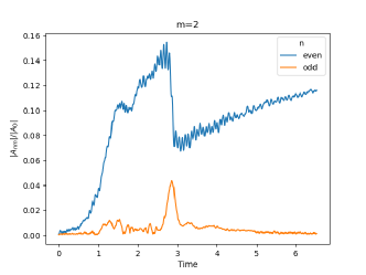
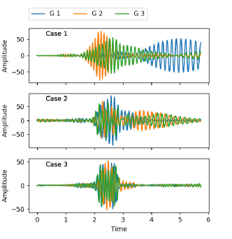
Figure 13: Top panel: total quadrupole ($m=2$) amplitude as a function of time for basis functions symmetric (blue) and anti-symmetric (orange) about the disc midplane. The vertical-horizontal resonance begins at $T\approx 2$ and culminates with jump in anti-symmetric power at $T\approx 2.9$. This is followed by a period of increasing bar amplitude that correlates with trapping orbits into vertical resonance. Finally, the vertically anti-symmetric asymmetry decays as the orbits lose phase coherence. Remaining panels: the first three PC groups in the M-SSA analysis of the first 8 kinematic Laguerre coefficients joined with the first 6 vertically symmetric BFE coefficients (Case 1), joined with the first 6 vertically anti-symmetric BFE coefficients (Case 2) and the Laguerre coefficients alone (Case 2). The first two analyses yield nearly identical PCs. The first two PCs represent 50% of the total power.

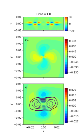
Figure 14: The density reconstruction $\rho$ on the $x$–$z$ plane (top), $\rho v_{z}$ (middle) and velocity $v_{z}$ (bottom) for PC1 at $T=3.0$ in Case 2. This reveals an ensemble of bar orbits that describe a correlated vertical oscillations as they circulate through the bar. PC2 (not shown) describes the same pattern. Logarithmically spaced contours of disc surface density are overlaid in the bottom panel for comparison.

6 Discussion and summary

This paper proposes a general approach for discovering dynamical mechanisms in simulations using a combination of basis-function expansions (BFEs) and multichannel singular spectrum analysis (M-SSA), with the possibility of additional time series describing associated field data such as kinematics, age or chemical data. While our examples are simulations that use the BFE method for solution of the Poisson equation, any set of simulation snapshots may be post processed to generate BFE coefficients.

We applied these ideas several situations that we have already studied in detail as method tests. We were pleasantly surprised that M-SSA not only recovered and reconfirmed our prior results, it provided new discoveries and insights. Our use of M-SSA on BFE time series of coefficients might be considered a form of unsupervised learning. We emphasise that no prior information about the spatial or temporal nature of these dynamics are included in our analysis: the only tuning parameters are the length of the time series, mostly determined by the astronomical scenario itself, and the window length, which is chosen to be less than half of the entire duration and often smaller for computational expediency. M-SSA rediscovered the three epochs from Petersen, Weinberg & Katz (2019b) that were determined by conventional methods.

Simulations of disc galaxies reveal natural $m=1$ or seiche and $m=2$ frequencies in nearly all cases. The seiche excitation is less dramatic than a bar or spiral arms but rather looks like a central offset or lopsided density feature with a pattern slower than most orbital frequencies. When applied to a combination of $m=1$ and $m=2$ coefficients simultaneously, M-SSA revealed the same dynamics discovered by eye: namely that when the bar pattern frequency approaches the natural dipole frequency, the bar and the seiche exchange power. In addition, M-SSA discovered a slow retrograde oscillation of the disc that is excited by the $m=1$ and $m=2$ interaction. The pattern speed is very slow, corresponding to a gigayear period scaled to the Milky Way. Such modes were predicted by Weinberg (1994) but was not obvious in the simulation by eye. While the power in this slow retrograde mode is only 5% of the total, its detection is highly significant.

We show that BFE time series may be augmented by other quantities. Kinematic data, which are easy to compute from simulations and observe directly from spectroscopic surveys, are included here using a Fourier-Laguerre expansion of the cylindrical velocity vector. We show that the spatial and kinematic data reinforce each other as we expect they should given the nature of phase space. Moreover, the vertical velocity field combined with anti-symmetric terms of the disc expansion basis allow clear description of the bar ‘buckling’ phenomenon.

Although we have not explored additional field data besides kinematic here, many codes simulate star formation and track chemical and stellar age data. These fields may be easily added to investigate the coupling between chemical and star formation patterns and specific dynamical mechanisms such as minor mergers, spiral arm or bar formation. Other promising time series include conserved quantities of particular orbit ensembles such as approximate action values or energies in order to test or elicit dynamical mechanisms.

Our implementation of of M-SSA for these tests is standard and other publicly available implementations can be found in several published packages, such as The Singular Spectrum Analysis - MultiTaper Method (SSA-MTM) distributed by the Department of Atmospherical and Oceanographic Sciences at UCLA, commercial packages, among others. Our implementation naturally interfaces with our EXP code (Petersen, Weinberg & Katz, 2019a) and integrated tools will be provided as part of an upcoming public release.

Data availability statement

The simulation data underlying this article will be shared on reasonable request to the corresponding author. All other data underlying this article are available in the article.

References

- Abramowitz & Stegun (1964) Abramowitz M., Stegun I. A., 1964, Handbook of Mathematical Functions. National Bureau of Standards, Washington
- Binney & Tremaine (2008) Binney J., Tremaine S., 2008, Galactic Dynamics: Second Edition. Princeton
- Clutton-Brock (1972) Clutton-Brock M., 1972, Ap&SS, 16, 101
- Clutton-Brock (1973) Clutton-Brock M., 1973, Ap&SS, 23, 55
- Debattista et al. (2006) Debattista V. P., Mayer L., Carollo C. M., Moore B., Wadsley J., Quinn T., 2006, ApJ, 645, 209
- Earn (1996) Earn D. J. D., 1996, ApJ, 465, 91
- Fridman & Polyachenko (1984) Fridman A. M., Polyachenko, 1984, Physics of Gravitating Systems II. Springer-Verlag, New York
- Ghil & Vautard (1991) Ghil M., Vautard R., 1991, Nature, 350, 324
- Golub & Loan (1996) Golub G. H., Loan C. F. V., 1996, Matrix Computations, 3rd edn. The John Hopkins University Press, Baltimore, MD, pp. 56–57
- Golyandina & Zhigljavsky (2013) Golyandina N., Zhigljavsky A., 2013, Singular Spectrum Analysis for Time Series. Springer
- Groth & Ghil (2015) Groth A., Ghil M., 2015, Journal of Climate, 28, 7873–7893
- Gu & Eisenstat (2006) Gu M., Eisenstat S. C., 2006, SIAM J. Matrix Anal. Appl., 16(1), 79–92. (14 pages), 16, 79
- Hernquist & Ostriker (1992) Hernquist L., Ostriker J. P., 1992, ApJ, 386, 375
- Hill (1954) Hill E. L., 1954, Am. J. Phys., 22, 211
- Hohl (1971) Hohl F., 1971, ApJ, 168, 343
- Kalantari & Hassani (2019) Kalantari M., Hassani H., 2019, Forcasting, 1, 189
- Lilley, Sanders & Evans (2018) Lilley E. J., Sanders J. L., Evans N. W., 2018, MNRAS, 478, 1281
- Lilley et al. (2018) Lilley E. J., Sanders J. L., Evans N. W., Erkal D., 2018, MNRAS, 476, 2092
- Lloyd (1982) Lloyd S. P., 1982, IEEE Transactions on Information Theory, 28, 129
- Lorenz (1956) Lorenz E. N., 1956, Empirical orthogonal functions and statistical weather prediction. Tech. rep., M.I.T.
- M. Ghil et al. (2002) M. Ghil M. et al., 2002, Rev. Geophys., 40, 1.1
- Petersen & Weinberg (2020) Petersen M. S., Weinberg M. D., 2020, MNRAS, in preparation
- Petersen, Weinberg & Katz (2019a) Petersen M. S., Weinberg M. D., Katz N., 2019a, arXiv e-prints, arXiv:1902.05081
- Petersen, Weinberg & Katz (2019b) Petersen M. S., Weinberg M. D., Katz N., 2019b, arXiv e-prints, arXiv:1903.08203
- Petersen, Weinberg & Katz (2019c) Petersen M. S., Weinberg M. D., Katz N., 2019c, MNRAS, 490, 3616
- Quillen (2007) Quillen A., 2007, The Astronomical Journal, 124, 722
- Raha et al. (1991) Raha N., Sellwood J. A., James R. A., Kahn F. D., 1991, Nat, 352, 411
- Sellwood & Gerhard (2020) Sellwood J. A., Gerhard O., 2020, MNRAS, 495, 3175
- Sridhar & Touma (1996) Sridhar S., Touma J., 1996, Monthly Notices of the Royal Astronomical Society, 279, 1263
- Watson (1966) Watson G. N., 1966, A Treatise on the Theory of Bessel Functions. Canbridge University Press
- Weinberg (1994) Weinberg M. D., 1994, ApJ, 421, 481
- Weinberg (1998) Weinberg M. D., 1998, MNRAS, 297, 101
- Weinberg (1999) Weinberg M. D., 1999, AJ, 117, 629