Strongly lensed candidates from the HSC transient survey

We present a lensed quasar search based on the variability of lens systems in the Hyper Suprime-Cam (HSC) transient survey. Starting from 101,353 variable objects with i-band photometry in the HSC transient survey, we used a variability-based lens search method measuring the spatial extent in difference images to select potential lensed quasar candidates. We adopted conservative constraints in this variability selection and obtained 83,657 variable objects as possible lens candidates. We then ran Chitah, a lens search algorithm based on the image configuration, on those 83,657 variable objects, and 2,130 variable objects were identified as potential lensed objects. We visually inspected the 2,130 variable objects, and seven of them are our final lensed quasar candidates. Additionally, we found one lensed galaxy candidate as a serendipitous discovery. Among the eight final lensed candidates, one is the only known quadruply lensed quasar in the survey field, HSCJ095921+020638. None of the other seven lensed candidates have been previously classified as a lens nor a lensed candidate. Three of the five final candidates with available Hubble Space Telescope (HST) images, including HSCJ095921+020638, show clues of a lensed feature in the HST images. We show that a tightening of our variability selection criteria might result in the loss of possible lensed quasar candidates, especially the lensed quasars with faint brightness or narrow separation, without efficiently eliminating the non-lensed objects; Chitah is therefore important as an advanced examination to improve the lens search efficiency through the object configuration. The recovery of HSCJ095921+020638 proves the effectiveness of the variability-based lens search method, and this lens search method can be used in other cadenced imaging surveys, such as the upcoming Rubin Observatory Legacy Survey of Space and Time.

1 Introduction

Strong gravitational lensing is a useful tool to study the Universe. Particularly, strong lensing of quasars can be used to study various topics in astrophysics and cosmology, such as the formation and evolution of supermassive black holes (e.g. Fan et al. 2019), quasar host properties (e.g. Peng et al. 2006; Ding et al. 2017), and the substructure of dark matter (e.g. Gilman et al. 2019; Nierenberg et al. 2020). Moreover, combined with the time delays between lensed images, lensed quasars can be used to measure the Hubble constant, $H_{0}$, which is crucial for examining cosmological models and probing dark energy (e.g. Wong et al. 2020; Chen et al. 2019).

Enlarging the sample of lensed quasars is important for further studies, and there have been several systematic searches looking for lensed quasars. The Cosmic Lens All Sky Survey (CLASS; Myers et al. 2003; Browne et al. 2003) is the first systematic lensed quasar search in radio wavelengths. CLASS identified lensed quasars by looking for resolved multiple images in high-resolution radio images of sources that were preselected to have flat spectra. In the optical, a large sample of lensed quasars has been constructed in the SDSS Quasar Lens Search (SQLS; Oguri et al. 2006; Inada et al. 2008, 2010, 2012; More et al. 2016a). Starting with spectroscopic confirmed SDSS quasars, SQLS applied morphological and colour selections to find lens candidates. Nowadays, thanks to multiple large-scale surveys with a higher spatial resolution, larger covering area, and/or increased depth, more and more lensed quasars have been found, and new lens search methods have been developed with the aim to take advantage of those new surveys, such as catalogue exploration techniques (e.g. Agnello et al. 2015; Agnello 2017; Ostrovski et al. 2017; Williams et al. 2017; Rusu et al. 2019), and inspections of the image configurations (e.g. Agnello et al. 2015; Chan et al. 2015). Citizen science is also useful for lensed quasar searches (Marshall et al. 2016; More et al. 2016b; Sonnenfeld et al. 2020).

The Gaia all-sky survey provides new approaches for lensed quasar searches. In combination with other surveys, such as SDSS, PanSTARRS (e.g. Lemon et al. 2017, 2018, 2019; Ostrovski et al. 2018), DES (e.g. Agnello et al. 2018; Agnello & Spiniello 2019), CRTS (e.g. Krone-Martins et al. 2019), one could search for lensed quasars by looking for Gaia multiplets or by comparing their flux and position offsets. One could also apply machine learning techniques to look for lensed quasars within Gaia (Delchambre et al. 2019).

Since quasars are variable sources, it is possible to conduct lensed quasar searches through the exploitation of their variability. A cadenced survey is ideally designed to reveal this variability through difference imaging. Kochanek et al. (2006) first proposed using difference imaging to find lensed quasars: while most of the (non-lensed) variable objects are point-like sources, lensed quasars with a sufficient angular size may appear as extended variable objects in the difference images. Specifically, lensed quasars whose image separations are comparable to the size of the point-spread function (PSF) appear as extended objects. Small quasar-image separations (relative to the PSF) lead to point-like objects, whereas large quasar-image separations lead to multiple point-like objects in the difference image. Therefore, the objects that exhibit an extended feature or have multiple point features in the difference images are potential lenses. As a cadenced survey, the upcoming Rubin Observatory Legacy Survey of Space and Time (LSST) will provide not only a huge pool of thousands of new lensed quasars (Oguri & Marshall 2010, hereafter OM10), but also a great opportunity to apply the time variability for a lens search.

In this work, we conduct a lensed quasar search by applying the variability-based method described in Chao et al. (2020, hereafter C20) to the HSC transient survey (Yasuda et al. 2019). The HSC transient survey is an ongoing cadenced survey of the Subaru Telescope (Miyazaki et al. 2018a), and it has a similar image quality as expected for the LSST. The final candidates of lensed quasars here undergo a three-step process: (1) a variability-based selection (C20) according to their spatial extent in the difference images of the HSC transient survey; (2) classification as potential lenses by Chitah (Chan et al. 2015), a lens search algorithm examining the image configuration through lens modelling; and (3) visual inspection.

The organisation of this paper is as follows. In Sec. 2, we introduce the data from the HSC transient survey used in this work. We describe our lens selection method in Sec. 3. Sec. 4 shows the lens selection results, followed by our conclusions in Sec. 5.

2 The HSC transient survey

The HSC transient survey has observed the COSMOS (Scoville et al. 2007) field as part of the HSC-SSP (Subaru Strategic Program; Aihara et al. 2018; Miyazaki et al. 2018b; Komiyama et al. 2018; Kawanomoto et al. 2018; Furusawa et al. 2018) from November 2016 to June 2017, covering 1.77 $\text{deg}^{2}$ in the UltraDeep layer with a pixel size of 0.168$\arcsec$. There are 8, 9, 13, 14, and 11 epochs (i.e. nights of observations) in the g-, r-, i-, z-, and y- bands, respectively, with median depths of g=26.4 mag, r=26.3 mag, i=26.0 mag, z=25.6 mag, and y=24.6 mag. For the difference imaging, the HSC transient survey uses the methods in Alard & Lupton (1998) and Alard (2000).

Before we proceeded to the lens search with the difference images, we first selected ‘HSC variables’ from the HSC transient survey. An HSC variable is defined in C20 as an object that is detected on the difference images at least twice in the HSC transient survey – the detections could be from two different epochs or two different bands. Following C20, we focussed on the HSC variables that have difference images in the i-band, as the simulation and lens search algorithm have been developed for the i-band in C20. From 2,252,293 sources contained in the COSMOS field (Capak et al. 2007; Ilbert et al. 2009), we picked out 101,353 sources with HSC i-band difference images by requiring at least two detections in the HSC transient survey.

3 Selection method

We selected lensed quasars in three steps. We first performed the variability-based selection among 101,353 HSC variables (Sec. 2) with their i-band difference images, which is described in Sec. 3.1. After the variability-based selection, we ran Chitah (Chan et al. 2015), a lens search method based on the image configuration that is described in Sec. 3.2. Finally, we visually inspected the remaining HSC variables and graded them according to the scheme described in Sec. 3.3. The HSC variables with the highest scores are our final lensed quasar candidates. In this work, we focus on quadruply lensed quasars (quad).

3.1 Variability-based selection

The variability-based lens search method described in C20 quantifies the spatial extent of HSC variables on the i-band difference images, and it selects the HSC variables with a large spatial extent as lensed quasar candidates. Briefly, the steps of this method are as follows:

1. Create the ‘3$\sigma$-mask’ for each HSC variable, $m$, in each epoch, $t$, by defining

   $$I^{m}_{\text{mask},t}(i,j)=\cases{1},&\text{if }|I^{m}_{t}(i,j)|>3\sigma^{m}_{t}(i,j)\\ 0,\text{otherwise}{}$$ (1)

   where $i=1,...,N_{x}$ and $j=1,...,N_{y}$ are the pixel indices in the difference image cutout $I^{m}_{t}(i,j)$ of dimensions $N_{x}\times N_{y}$, and $\sigma^{m}_{t}(i,j)$ are the estimated 1-$\sigma$ uncertainties in the difference image cutout. Pixels $(i,j)$ with $I^{m}_{\text{mask},t}(i,j)=1$ are the pixels in the 3$\sigma$-mask.

2. Define the ‘effective region’, $I^{m}_{\text{eff},t}(i,j)$, and the area of the effective region, $A^{m}_{\text{eff},t}$, for each HSC variable $m$ in each epoch $t$ by

   $$I^{m}_{\text{eff},t}(i,j)=\cases{1},&\text{if }\displaystyle\sum_{i^{\prime}=i-1}^{i+1}\sum_{j^{\prime}=j-1}^{j+1}I^{m}_{\text{mask},t}(i^{\prime},j^{\prime})>2\\ 0,\text{otherwise}{}$$ (2)

   and

   $$A^{m}_{\text{eff},t}=\sum\limits_{i=1}^{N_{x}}\sum\limits_{j=1}^{N_{y}}I^{m}_{\text{eff},t}(i,j).$$ (3)

   where $A^{m}_{\text{eff},t}$ is equivalent to the number of pixels with pixel values equal to one in the effective region ($I^{m}_{\text{eff},t}=1$). While the 3$\sigma$-mask includes many isolated single pixels which are actually noise peaks, the effective region area, $A^{m}_{\text{eff},t}$, is a more accurate quantification of the object’s spatial extent in the difference image.

3. Compute $A_{\text{eff},t}(p_{\text{thrs}}\%)$ as the effective region area for each epoch $t$ such that $p_{\text{thrs}}\%$ of the HSC variables have values $A^{m}_{\text{eff},t}<A_{\text{eff},t}(p_{\text{thrs}}\%)$. If an HSC variable $m^{\prime}$ is not observed in an epoch $t^{\prime}$, $A^{m^{\prime}}_{\text{eff},t^{\prime}}=0$ would be assigned. For such case, we did not include it when we computed $A_{\text{eff},t}(p_{\text{thrs}}\%)$.

4. Set a threshold on the number of epochs, $N_{\text{thrs}}$, such that an HSC variable $m$ is selected as a lensed quasar candidate if it satisfies

   $$A^{m}_{\text{eff},t}>A_{\text{eff},t}(p_{\text{thrs}}\%)$$ (4)

   for more than $N_{\text{thrs}}$ epochs. Table 1 shows the dates and seeings of all the 13 epochs in the i-band.

For the first application of C20, we employed very loose constraints, $p_{\text{thrs}}\%=50\%$ and $N_{\text{thrs}}=0$, to select lensed quasar candidates. Among the 101,353 HSC variables, 83,657 HSC variables were identified as lensed quasar candidates by the variability-based selection. The variability-based selection did not bring down the number of potential lensed quasar candidates substantially due to these loose constraints. However, the variability-based selection is important for finding lensed quasars. Lensed quasars are not only variable, but also multiple point-like or extended if not deblended. These loose constraints already discarded part of the contaminations, such as some single point-like variables and false detections, and shall become more stringent if we attempt to find lensed quasars with the variability-based lens search algorithm in a field that is much larger than COSMOS. By properly tightening the constraints in the variability-based selection, we will be able to improve the lens search efficiency (see the discussion in Sec. 4.4).

Table 1: HSC transient survey observation dates and seeings in the i-band.

Epochs/Observation dates	Seeing (arcsec)
2016-11-25	0.83
2016-11-29	1.16
2016-12-25	1.25
2017-01-02	0.68
2017-01-23	0.70
2017-01-30	0.76
2017-02-02	0.48
2017-02-25	0.72
2017-03-04	0.69
2017-03-23	0.66
2017-03-30	0.98
2017-04-26	1.24
2017-04-27	0.58

3.2 CHITAH

For the 83,657 lensed quasar candidates selected in Sec. 3.1, we ran Chitah on their stacked images from the HSC survey (g-, r-, i-, z-, and y-bands) to reduce the number of lensed quasar candidates. Briefly, Chitah works as follows: (1) picking two image cutouts, one from the bluer bands (g/r) and one from the redder bands (z/y) which have sharper PSFs; (2) matching PSFs in the two selected bands; (3) decomposing the image cutouts into $P$ and $Q$, the former for the lens galaxy and the latter for the lensed images, according to colour information; (4) estimating the lens photo-centre using the light distribution on $P$ and identify the lensed image positions on $Q$ with four PSFs; and (5) using the lensed image positions identified on $Q$ to model the lens mass distribution with a singular isothermal ellipsoid (SIE) model (Kormann et al. 1994).

The outputs of the model are the best-fitting SIE parameters: the Einstein radius ($\theta_{\text{Ein}}$), the axis ratio ($q$), the position angle (PA), and the centre of mass (of the lens). The convergence $\kappa$ of the SIE model is given by

$$\kappa(\theta_{1},\theta_{2})=\frac{\theta_{\text{Ein}}}{2\sqrt{\theta^{2}_{1}+\theta^{2}_{2}/q^{2}}},$$ (5)

where $(\theta_{1},\theta_{2})$ are the coordinates relative to the centre of mass along the semi-major and semi-minor axes of the elliptical mass distribution. We determineed the SIE parameters by minimising the $\chi^{2}_{\text{source}}$ on the source plane, which is defined as

$$\chi^{2}_{\text{source}}=\sum\limits_{n}\frac{|\mathbf{r}_{n}-\mathbf{r}_{\text{model}}|^{2}}{\sigma^{2}_{\text{image}}/\mu_{n}},$$ (6)

where $\mathbf{r}_{n}$ is the respective source position mapped from the position of lensed image $n$ by the SIE lens model, $\mu_{n}$ is the magnification of lensed image $n$ from the SIE lens model, $\sigma_{\text{image}}$ was chosen to be the HSC pixel size (0.168″) as an estimate of the uncertainty, and $\mathbf{r}_{\text{model}}$ is the modelled source position that is evaluated by a weighted mean of $\mathbf{r}_{n}$ (Oguri 2010),

$$\mathbf{r}_{\text{model}}=\frac{\sum\limits_{n}\sqrt{\mu_{n}}\mathbf{r}_{n}}{\sum\limits_{n}\sqrt{\mu_{n}}}.$$ (7)

Here the index $n$ runs from one to four for quads in this work. We also used the lens photo-centre, $\mathbf{x}_{\text{centre}}$, from the light distribution on $P$ as a prior to constrain the centre of mass of the SIE model, $\mathbf{x}_{\text{model}}$ . Therefore, we define

$$\chi^{2}_{\text{centre}}=\frac{|\mathbf{x}_{\text{model}}-\mathbf{x}_{\text{centre}}|^{2}}{\sigma^{2}_{\text{centre}}},$$ (8)

where $\sigma_{\text{centre}}$ was chosen to be the same as $\sigma_{\text{image}}$. We further took into account the residuals of the fit to the lensed quasar image from Chitah. The difference between the lensed image, $Q(i,j)$, and the predicted image formed by four PSFs, $Q^{\text{P}}(i,j)$, is defined as

$$\chi^{2}_{\text{residual}}=\sum\limits_{i,j}\frac{\left[Q(i,j)-Q^{\text{P}}(i,j)\right]^{2}}{var(i,j)},$$ (9)

where $i=1,...,N_{x}$ and $j=1,...,N_{y}$ are the pixel indices in the image cutout of dimensions $N_{x}\times N_{y}$, and $var(i,j)$ is the pixel uncertainty in $Q(i,j)$. In this work, we assume that $var(i,j)$ is constant and thus irrelevant in the minimisation for the point source positions. We note that $Q^{\text{P}}$ was obtained from the four PSFs fitting in order to identify the lensed image positions, which is independent of lens modelling. Therefore, the fitted fluxes of lensed images allow for the presence of image flux anomalies.

The criteria for the classification of lensed quasar candidates are

$$\chi^{2}=\chi^{2}_{\text{source}}+\chi^{2}_{\text{centre}}<1$$ (10)

and

$$\chi^{2}_{\text{residual}}<2.$$ (11)

These two criteria allow CHITAH to extract a manageable number of candidates and a low false-positive rate ($<3\%$, see Figure 1 in Chan et al. (2015)). We note that the second criterion (Eq. 11) is chosen empirically due to the arbitrary scale in the pixel uncertainty. Consequently, this loose constraint discarded only $\approx 2\%$ of the objects while most of the objects ($\approx 95\%$) were eliminated by Eq. 10. The lensed candidates were selected by $0.3\arcsec<\theta_{\text{Ein}}<2\arcsec$ and $q>0.2$. After running Chitah, we reduced the number of the lensed quasar candidates from 83,657 to 2,130.

3.3 Visual inspection

We visually inspected the remaining 2,130 lensed quasar candidates. We first discarded 2,065 lensed quasar candidates that are obviously not lenses. Three of the coauthors then independently graded each of the 65 remaining lensed quasar candidates with the following grading scheme:

• 3: definite lens,

• 2: probable lens,

• 1: likely lens, and

• 0: not a lens.

The visual inspection was mainly conducted with the HSC colour-composite images. Typical aspects taken into consideration in grading are the colour difference between the possible lensed images and the possible lens galaxy, and the positions of the possible lensed images. This grading scheme is the same as the one on the SuGOHI lens sample from the HSC survey (e.g. Sonnenfeld et al. 2018; Wong et al. 2018; Chan et al. 2020; Jaelani et al. 2020). We then took the average score among the three graders for each lensed quasar candidate, and the candidates with average scores higher than 1.5 would be our final lensed quasar candidates. We note that in visual inspection, the gradings are based on general lensed features, which are not specific to lensed quasars. In total, we have eight candidates with an average score higher than 1.5 (listed in Table 2). Further properties of the eight final candidates are listed in Table 3. One of our eight final candidates was found by chance (See Sec. 4.1).

Table 2: Candidates with average scores higher than 1.5 in visual inspection.

Name	RA (deg)	DEC (deg)	Average score	Comment
HSCJ095921+020638	149.84071	2.11068	3.0	Anguita et al. (2009)
HSCJ100050+013251	150.20947	1.54775	2.3	Probable lensed galaxy
HSCJ095921+025700	149.84037	2.95013	2.0	Probable lensed galaxy. No HST image
HSCJ100307+020241	150.78256	2.04484	1.7	No HST image
HSCJ095943+022046	149.93252	2.34623	1.7
HSCJ095744+023835	149.43571	2.64332	1.7
HSCJ100050+031825	150.21200	3.30706	1.7	No HST image
HSCJ100129+024427	150.37457	2.74093	2.0	Lensed galaxy candidate by serendipitous discovery

Table 3: Variability selection and Chitah properties of the candidates listed in Table 2.

Name	Number of	$\chi^{2}_{\text{residual}}$	$\chi^{2}$	$\theta_{\text{Ein}}$	q	$\theta^{\text{s}}_{\text{Ein}}$
	variability epochs			[$\arcsec$]		[″]
HSCJ095921+020638	7	0.000357	0.4	0.7	0.95	0.7
HSCJ100050+013251	6	0.013854	0.7	1.1	0.90	1.0
HSCJ095921+025700	1	0.005372	1.0	1.2	0.64	0.9
HSCJ100307+020241	7	0.001768	1.0	1.1	0.57	0.8
HSCJ095943+022046	8	0.000225	0.3	0.9	0.75	0.8
HSCJ095744+023835	5	0.000332	0.6	1.1	0.88	1.0
HSCJ100050+031825	7	0.002117	0.3	1.0	0.89	0.9
HSCJ100129+024427	0	0.003324	0.7	0.9	0.96	0.9

4 Results and discussion

In this section, we take a further look at the HSC variables that were selected by our approach. We describe the final candidates in Sec. 4.1. In Sec. 4.2, we discuss the objects selected as candidates by both the variability selection and Chitah, but rejected by our visual inspection. The discussion about the objects that meet the variability selection criteria but get rejected by Chitah is in Sec. 4.3.We compare our lens candidates to previously identified candidates from other searches in Sec. 4.4.

4.1 Final candidates

We show the eight final candidates in Fig. 1 and Table 2. The highest scored candidate, HSCJ095921+020638, is a known lensed quasar (Anguita et al. 2009). The recovery of HSCJ095921+020638 demonstrates the effectiveness of our variability-based lens searching method.

HSCJ095921+025700 was picked out by the variability selection due to the loose criteria ($p_{\text{thrs}}\%=50\%$ and $N_{\text{thrs}}=0$). Under these loose criteria, an HSC variable can be selected as long as it has a non-zero effective region in one of a few specific epochs, even if the effective region comes from the accumulation of noise peaks. These objects that were selected due to possible noise peaks and further identified as lens candidates by their image configuration in colour-composite images are more likely to be lensed galaxy candidates, instead of lensed quasar candidates. Although the loose criteria are sensitive to noise peaks, they are still sufficient for the COSMOS field we examine in this work, given the covering area of the COSMOS field. Moreover, the loose criteria allow us to have a more complete sample that includes lensed quasars with a faint brightness or small separation.

Most of the other final candidates have substantial effective region areas satisfying the loose criteria in the variability selection, and also show a possible lens feature such as a colour gradient in the colour-composite images. Thanks to a fortunate mistake, our variability-based method picked up HSCJ100129+024427 in an earlier version of our code. HSCJ100129+024427 has a zero effective region area across all the 13 epochs, and the final variability selection actually did not pick it out. Given its lens-like appearance, we keep this system for further investigation: Chitah identifies the lensing feature of HSCJ100129+024427, followed by an average score of probable lens from the visual inspection. Therefore, HSCJ100129+024427 is more likely a candidate of a lensed galaxy, instead of a candidate of a lensed quasar.

We show archival Hubble Space Telescope (HST) F814W images of HSCJ095921+020638, HSCJ100129+024427, HSCJ095943+022046, and HSCJ095744+023835 (HST proposal id: 9822; PI: Scoville) in Fig. 3 (Koekemoer et al. 2007), and the HST F105W image of HSCJ100050+013251 (HST proposal id: 14808; PI: Suzuki) in Fig. 4. From the HST images, we can clearly see the four multiple images in HSCJ095921+020638 (top-left panel in Fig. 3), and three possible lensed images in HSCJ100129+024427 (top-right panel in Fig. 3). We also see the possible arc feature in HSCJ100050+013251 (Fig. 4), indicating that this system is likely to be a lensed galaxy. On the other hand, the lensed features of HSCJ095943+022046 and HSCJ100050+031825 are hard to see, and these two objects are more likely to be spiral galaxies or galaxies with dust lanes.

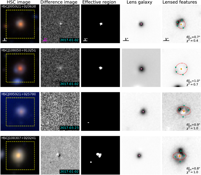
Figure 1: Final candidates, the variable objects identified as lensed quasars by both the variability-based method and Chitah with average scores higher than 1.5 from the visual inspection. The first column shows the gri image of each final candidate. The second column shows their difference images at the epoch at which they met the time variability selection criteria, and the third column shows their corresponding effective region, a quantification of the object’s spatial extent in the difference image. The fourth column shows the lens galaxy predicted by Chitah with the lens centre marked by the magenta cross. The fifth column shows their predicted lensed features by Chitah with their best-fit SIE model. The positions of the fitted lensed images are in green dots, the predicted source position is labelled as the yellow diamond, and the red curves are the critical and caustic curves of their best-fit SIE model. The variability-based selection uses cutouts of 10$\arcsec$ $\times$ 10$\arcsec$ (first three columns), and Chitah uses cutouts of 7$\arcsec$ $\times$ 7$\arcsec$, which is the yellow dashed box in the first column.

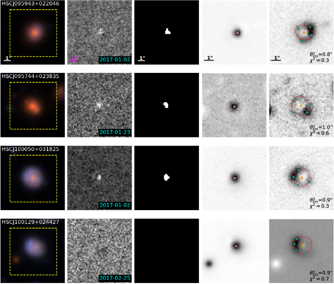
Figure 2: HSCJ100129+024427 is a serendipitous discovery and is more likely to be a candidate of a lensed galaxy due to the zero effective region area across all 13 epochs. See Sec. 4.1 for details.

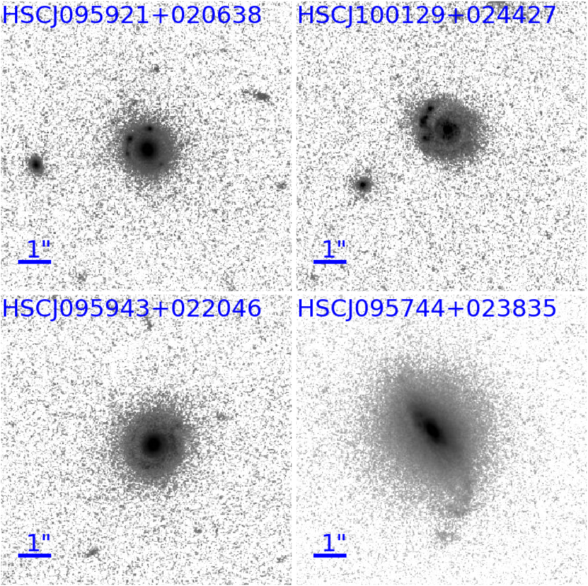
Figure 3: HST F814W images of four final candidates. HSCJ095921+020638 (top left) is the only known quadruply lensed quasar in the COSMOS field.

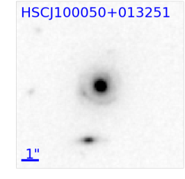
Figure 4: HST F105W image of HSCJ100050+013251, a possible lensed galaxy. The possible arc is clearly visible.

4.2 Chitah false positives

In Fig. 5, we show examples of the objects that get selected by both the variability-based selection and Chitah, but rejected in the visual inspection. Those objects are called Chitah false positives in this work.

These objects are classified as non-lenses based on visual inspection as they do not exhibit typical morphologies of lenses. For example, the system HSCJ100129+020620 does not show lens-like arcs in the colour images, and the system HSCJ100244+015514 is probably a ring galaxy (with the ring being physically associated with the central galaxy) since the morphology of the ring is unlikely to be formed by lensing. Actually, both HSCJ100129+020620 and HSCJ100244+015514 at only one epoch have effective regions larger than $A_{\text{eff},t}(p_{\text{thrs}}\%=50\%)$, and their effective regions are only 1-2 pixels at those epochs (December 25, 2016 and March 30, 2017, respectively). Moreover, the effective region of HSCJ100129+020620 more likely comes from noise peaks. Although Chitah might misidentify kinds of objects such as HSCJ100129+020620 and HSCJ100244+015514, applying stricter criteria in the variability-based selection (higher values for $p_{\text{thrs}}\%$ or $N_{\text{thrs}}$) can avoid such misidentification. However, we might lose the candidates of faint or small-separation lensed quasars by doing so.

Compared to the final candidates and to the other Chitah false positives, HSCJ100226+005858 exhibits a different colour in the gri-composite image, and it has a rather round and compact shape. In fact, HSCJ100226+005858 is classified as a star in the internal HSC transient catalogue (Yasuda et al. 2019). HSCJ100226+005858 is probably a variable star or a star that is too bright for the transient pipeline to subtract the light perfectly since it has substantial amounts of the effective regions across almost all eight epochs at which it has been observed in the i-band (see Sec. 4.3 for detail).

The nearly monotone colour of HSCJ100332+013852 indicates that it is unlikely to be a lensed object. From the gri-composite image, HSCJ100332+013852 is likely a merger of two or more galaxies. Such a merger process might trigger AGN activity that results in effective regions passing our selection criteria.

HSCJ100319+021447 shows a possible tidal feature around the top right, and the possible tidal event could be the reason for the variable brightness given previous studies that indicate mergers could trigger AGN activity and show tidal features (e.g. Ellison et al. 2011, Silverman et al. 2011, Capelo et al. 2015, Comerford et al. 2015, Stemo et al. 2020). Moreover, Chitah identifies the blue trait around this possible tidal feature as the lensed images in HSCJ100319+021447, hence the misidentification of HSCJ100319+021447.

HSCJ095904+014812 is classified as a supernova in the internal HSC transient catalogue, and it exploded during the survey period in Table 1, resulting in the substantial effective region areas. Furthermore, the blue features in HSCJ095904+014812 are likely star-forming regions of a spiral galaxy, and these blue features cause the misidentification from Chitah. HSCJ095949+014141 is also classified as a supernova in the internal HSC transient catalogue. While HSCJ095949+014141 appears to be binary, Chitah misidentifies it as a lens because of the colour gradient in the bottom-right object (so part of the object is mistaken as lensed features) or imperfect PSF matching. Additionally, when checking the difference images and the effective regions of both HSCJ095904+014812 and HSCJ095949+014141, we found three stages: (1) before the exploding epochs, nothing was visible in the difference images and the corresponding effective region areas were also zero; (2) the effective region areas increased suddenly and significantly in an epoch, and continued to increase afterwards; (3) after the effective region areas reached a maximum in an epoch, the effective region areas started to decrease. These three stages are similar to a supernova, indicating that the effective region (Eq. 2) can also be used for the detection of supernovae. The combination of the variability-based selection and Chitah is even possible for the detection of lensed supernovae, though the detection might happen at a much later time after the explosion.

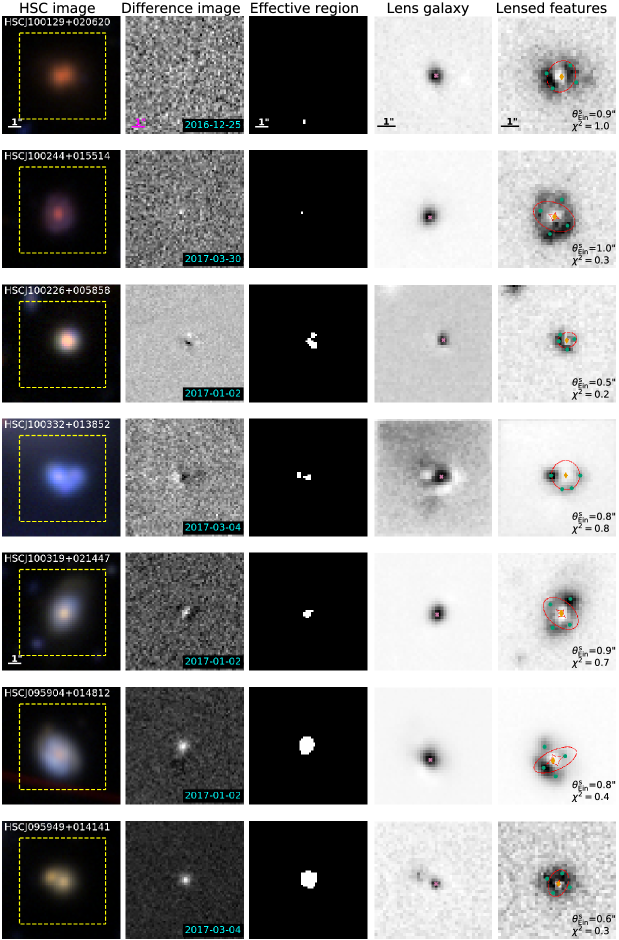
Figure 5: Examples of Chitah false positives, the variable objects identified as lensed quasars by both the variability-based method and Chitah, but rejected by the visual inspection. The five columns are in the same format as in Fig. 1. For details about these Chitah false positives, see Sec. 4.2.

4.3 Variability false positives

Here we examine the objects selected by the variability-based selection but rejected by Chitah, and we call these objects variability false positives in this work. Many of variability false positives have extremely large effective region areas across all the epochs, which are due to artificial effects, as the examples shown in Fig. 6. A misidentification such as the one in Fig. 6 could be prevented by assigning an upper limit to the effective region area. We can discard an HSC variable from the lens candidate selection if its effective region area exceeds the upper limit in a certain number of epochs since an abnormally large area of effective regions over many epochs suggests that heavy artificial effects happen around the HSC variable and that the detection of the HSC variable is not reliable. By doing so, however, we might miss lens candidates that are located close to artefacts.

Many variability false positives that are point-like have effective region areas that are even larger than most of our final candidates and the Chitah false positives, which means that we take the risk of losing promising lensed quasar candidates if we discard these variability false positives by applying stricter constraints on $p_{\text{thrs}}\%$ and $N_{\text{thrs}}$. We show some examples of these point-like variability false positives in Fig. 7. In particular, HSCJ095725+021832, HSCJ100042+022311, and HSCJ095821+020532 have ‘Taiji-like’ dipole patterns – half black and half white in the difference images. The Taiji-like patterns are possibly caused by the object brightnesses. From the simulation work done in C20, we found that an object starts to have the Taiji-like dipole residual in the difference images when it is brighter than $\lesssim$ 21.5 mag, regardless of whether the object is variable. The possible reason is that the transient pipeline no longer performs the image subtraction perfectly and it could not subtract the light correctly when an object is too bright ($\lesssim$21.5 mag). The brighter the object is, the more obvious the Taiji-like pattern is in the difference image. The Taiji-like residuals contribute larger effective region areas, and the variability-based selection would therefore misidentify these point-like objects as lensed quasar candidates. We note that, proper motions and parallaxes can also produce the Taiji-like pattern. While this effect should be negligible in the HSC transient survey, it will start to be visible in the 10-year survey of the LSST. Nonetheless, the Taiji-like pattern associated with proper motions and parallaxes of stars would change over time, and the multiple epochs of difference images in the LSST can help distinguish between proper motions of stars and the difference-image issue associated with bright objects.

In addition to those objects with Taiji-like residuals, some of the variability false positives could also be variable stars or unlensed quasars, such as HSCJ100159+025933 and HSCJ100041+030113. They are classified as a star and a quasar in the internal HSC transient catalogue, respectively. Although not listed in the internal HSC transient catalogue, HSCJ100055+030138 is possibly a variable star or an unlensed quasar as well. We inspected the difference images of 13 epochs, the corresponding effective regions, and the colour-composite images of HSCJ100055+030138 and found that its effective region areas might come from a substantial brightness change, instead of noise peaks or improper image subtraction. Ideally, lensed quasars have larger effective region areas due to their multiple images, and strict thresholds on the effective region areas for the variability selection should largely decrease the number of those point-like false positives, such as variable stars or unlensed quasars, without aggressively losing the lensed quasar candidates. However, in this work, our final candidates of lensed quasars generally have smaller effective regions than the Chitah false positives and the variability false positives. Although the loose constraints on the variability-based selection in this work yield a huge number of non-lensed objects, they seem to be necessary for securing the lensed quasar candidates. Therefore, Chitah is important as the second step in this lens search starting from time variability since it discards the point-like objects with large effective regions and efficiently decreases the number of lensed quasar candidates without missing the promising ones.

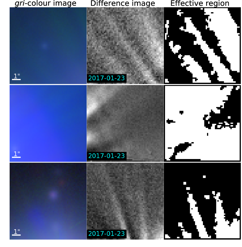
Figure 6: Artificial effects that were selected by the variability-based selection due to the extremely large effective regions.

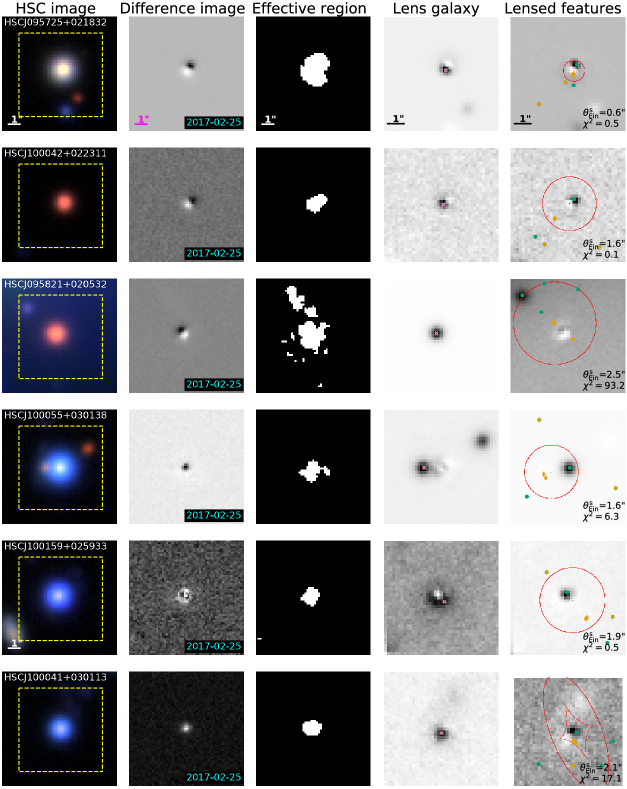
Figure 7: Examples of variability false positives, the variable objects identified as lensed quasars by the variability-based method, but rejected by Chitah. The columns are in the same format as in Fig. 1. See Sec. 4.3 for more details.

4.4 Discussion

We searched the literature to check if any of our final candidates have been found as a lens system. Except for HSCJ095921+020638, none of the other final candidates have been found as a lens. Among the final candidates, HSCJ100050+013251, HSCJ100307+020241, HSCJ095943+022046, and HSCJ095744+023835 are listed in the galaxy catalogue of Capak et al. (2007), and our serendipitous discovery, HSCJ100129+024427, is listed as a bright galaxy in the catalogue of Lilly et al. (2009). We also checked the WISE C75/R90 catalogues from Assef et al. (2018) and the Milliquas catalogue v7.1 (2021) (Flesch 2019). For C75 and R90, none of our final candidates are included. For Milliquas, only the known quad, HSCJ095921+020638, is included.

The recovery of the known lensed quasar, HSCJ095921+020638, and the discovery of the other final candidates can represent the completeness of our lensed quasar search, since we estimate that the number of quad(s) lying in the UltraDeep layer of the COSMOS field within the HSC transient survey (i $\sim$26.0 mag) is about $1\pm 1$ based on the lensing rates in OM10 and the correction in Spiniello et al. (2018). We further found that the strictest criterion for HSCJ095921+020638 to qualify the variability-based selection is $(p_{\text{thrs}}\%,N_{\text{thrs}})=(50\%,6)$. With this last criterion, the variability-based selection would identify 32,127 out of the 101,353 HSC variables as lensed quasar candidates, and 936 out of these 32,127 objects would further be identified as lensed quasar candidates by Chitah. In the end, under the same visual inspection, only four objects in Table 2 remain as final candidates: HSCJ095921+020638, HSCJ095943+022046, HSCJ095744+023835, and HSCJ100050+031825. We note that the COSMOS field is small and HSCJ095921+020638 is faint, so the loose constraints applied in this work to recover HSCJ095921+020638 might not be mandatory for a more general lensed quasar search in a larger field. In fact, C20 has demonstrated that we could find bright lensed quasars with a wide separation at true-positive rate of 90.1% and false-positive rate of 2.3% with $(p_{\text{thrs}}\%,N_{\text{thrs}})=(95\%,9)$. In future applications of this method to larger cadenced image surveys, the selection criteria are adjustable to balance between purity and completeness.

5 Conclusion

In this work, we performed a lensed quasar search within the HSC transient survey through the time variability of lensed quasars. We first used i-band difference images from the HSC transient survey to select objects with the variability-based method in C20 based on their spatial extent in the difference image. We ran Chitah, a lens search algorithm based on the image configuration, on the objects selected by the difference image. Finally, we visually inspected the objects that were both selected by the variability-based method and Chitah and graded them. We summarise the work as follows:

1. Among the 101,353 HSC variables, the variability-based method conservatively selected 83,657 HSC variables as potential lensed quasar candidates with loose criteria. Among the 83,657 HSC variables, Chitah further identified 2,130 as lensed quasar candidates. The visual inspection picked out seven from the 2,130 lensed quasar candidates as final candidates. In addition to the seven final candidates, we serendipitously found one lensed galaxy candidate.

2. As a first application, we used the variability-based method from C20 in a conservative manner. Although C20 method is helpful in selecting potential lensed quasar candidates by picking out objects with a larger spatial extent in the difference image, this work shows that our final candidates generally have a smaller spatial extent than the false positives, indicating that tightened criteria in the variability selection might not be an ideal means to improve the lens search efficiency in COSMOS.

3. Since using the variability-based method alone might not be efficient, Chitah is important as a further examination to remove the false positives from the variability selection through object configurations, especially for discarding those point-like false positives.

4. For future lensed quasar searches in larger sky areas, we could use stricter criteria for the variability-based method to reduce the false-positive rates. The only known lensed quasar in the field we have examined in this work, HSCJ095921+020638, is a special case of faint lensed quasars, and the loose constraints on the variability-based method exploited in this work to recover HSCJ095921+020638 are not indispensable.

As this work has shown, the variability-based lens search method from C20 is workable and could be applied to other cadenced imaging surveys, and a combination with other lens search techniques as an advanced check such as Chitah will improve the lens search efficiency. The upcoming LSST is expected to have a difference imaging process and image quality similar to the HSC transient survey, but covering a much larger sky area. Therefore, we expect to discover new lensed quasars in the LSST through variability-based searches.