GOCor: Bringing Globally Optimized Correspondence Volumes into Your Neural Network

Abstract

The feature correlation layer serves as a key neural network module in numerous computer vision problems that involve dense correspondences between image pairs. It predicts a correspondence volume by evaluating dense scalar products between feature vectors extracted from pairs of locations in two images. However, this point-to-point feature comparison is insufficient when disambiguating multiple similar regions in an image, severely affecting the performance of the end task. We propose GOCor, a fully differentiable dense matching module, acting as a direct replacement to the feature correlation layer. The correspondence volume generated by our module is the result of an internal optimization procedure that explicitly accounts for similar regions in the scene. Moreover, our approach is capable of effectively learning spatial matching priors to resolve further matching ambiguities. We analyze our GOCor module in extensive ablative experiments. When integrated into state-of-the-art networks, our approach significantly outperforms the feature correlation layer for the tasks of geometric matching, optical flow, and dense semantic matching. The code and trained models will be made available at github.com/PruneTruong/GOCor.

1 Introduction

Finding pixel-wise correspondences between pairs of images is a fundamental problem in many computer vision domains, including optical flow [16, 21, 24, 55, 56, 59], geometric matching [15, 39, 45, 46, 59], and disparity estimation [12, 35, 43, 65]. Most recent state-of-the-art approaches rely on feature correlation layers, evaluating dense pair-wise similarities between deep representations of two images. The resulting four-dimensional correspondence volume captures dense matching confidences between every pair of image locations. It serves as a powerful cue in the prediction of, for instance, optical flow. This encapsulation of dense correspondences has further achieved wide success within semantic matching [10, 13, 20, 26, 28, 29, 30, 47, 59], video object segmentation [11, 19, 42, 61], and few-shot segmentation [38, 62]. The feature correlation layer thus serves as a key building block when designing network architectures for a diverse range of important computer vision applications.

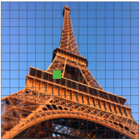
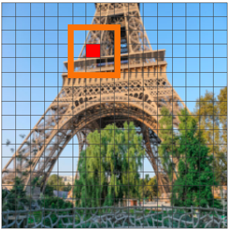
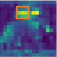
In the feature correlation layer, each confidence value in the correspondence volume is obtained as the scalar product between two feature vectors, extracted from specific locations in the two images, here called the reference and the query images. However, the sole reliance on point-to-point feature comparisons is often insufficient in order to disambiguate multiple similar regions in an image. As illustrated in Fig. 1, in the case of repetitive patterns, the feature correlation layer generates undistinctive and inaccurate matching confidences (Fig. 1d), severely affecting the performance of the end task. This remains the key limitation of feature correlation layers, since repetitive patterns, low-textured regions, and co-occurring similar objects are all pervasive in computer vision applications.

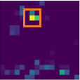
We design a new dense matching module, aiming to address the aforementioned issues by exploring information not exploited by the feature correlation layer. We observe that a confidence value in the correspondence volume generated by the feature correlation layer only depends on the feature vectors extracted at one pair of locations in the reference and query. However, the reference also contains the appearance information of other image locations, that are likely to occur in the query image. This includes the appearance of similar regions in the scene, opening the opportunity to actively identify and account for such similarities when estimating each matching confidence value. Moreover, the feature correlation layer ignores prior knowledge and constraints that can be derived from the query, e.g. the uniqueness and spatial smoothness of correspondences. Our matching module encapsulates the aforementioned information and constraints into a learnable objective function. Our enhanced correspondence volume is obtained by minimizing this objective during the forward-pass of the network. This allows us to predict globally optimised correspondence volumes, effectively accounting for similar image regions and matching constraints, as visualized in Fig. 1e.

Contributions: We introduce GOCor, a differentiable neural network module that generates the correspondence volume between a pair of images, acting as a direct replacement to the feature correlation layer. Our main contributions are as follows. (i) Our module is formulated as an internal optimization procedure that minimizes a customizable matching-objective during inference, thereby providing a general framework for effectively integrating both explicit and learnable matching constraints. (ii) We propose a robust objective that integrates information about similar regions in the scene, allowing our GOCor module to better disambiguate such cases. (iii) We introduce a learnable objective for capturing constraints and prior information about the query frame. (iv) We apply effective unrolled optimization, paired with accurate initialization, ensuring efficient end-to-end training and inference. (v) We perform extensive experiments on the geometric matching and optical flow tasks by integrating our module into state-of-the-art matching network architectures. We additionally show that our GOCor module can generalize to the dense semantic matching task. Our approach outperforms the feature correlation layer in terms of both accuracy and robustness. In particular, our GOCor module demonstrates better domain generalization properties.

(a) Reference image

(b) Query image

(c) Ideal Correlation

(d) Feat. Correlation

(e) GOCor (Ours)

Figure 1: Visualization of the matching confidences (c)-(e) computed between the indicated location (green) in the reference image (a) and all locations of the query image (b). The feature correlation (d) generates undistinctive and inaccurate confidences due to similar regions and repetitive patterns. In contrast, our GOCor (e) predicts a distinct high-confidence value at the correct location.

2 Related work

Enhancing the correlation volume: Since the quality of the correspondence volume is of prime importance, several works focus on improving it using learned post-processing techniques [31, 33, 47, 64]. Notably, Rocco et al. [47] proposed a trainable neighborhood consensus network, NC-Net, applied after the correlation layer to filter out ambiguous matches. Instead, we propose a fundamentally different approach, operating directly on the underlying feature maps, before the correlation operation. Our work is also related to [27, 48], which generate filters dynamically conditioned on an input [27] or features updated with an attentional graph neural network, whose edges are defined within the same or the other image of a pair [48]. Xiao et al. [63] also recently introduced a learnable cost volume that adapts the features to an elliptical inner product space.

Optimization-based meta-learning: Our approach is related to optimization-based meta-learning [4, 5, 6, 32, 60, 67]. In fact, our GOCor module can be seen as an internal learner, which solves the regression problem defined by our objective. In particular, we adopt the steepest descent based optimization strategy shown effective in [5, 6]. From a meta-learning viewpoint, our approach however offers a few interesting additions to the standard setting. Unlike for instance, in few-shot classification [4, 32, 67] and tracking [5, 60], our learner constitutes an internal network module of a larger architecture. This implies that the output of the learner does not correspond to the final network output, and therefore does not receive direct supervision during (meta-)training. Lastly, our learner module actively utilizes the query sample through the introduced trainable objective function.

3 Method

3.1 Feature Correlation Layers

The feature correlation layer has become a key building block in the design of neural network architectures for a variety of computer vision tasks, which either rely on or benefit from the estimation of dense correspondences between two images. To this end, the feature correlation layer computes a dense set of scalar products between localized deep feature vectors extracted from the two images, in the form of a four-dimensional correspondence volume. We consider two deep feature maps $f^{r}=\phi(I^{r})$ and $f^{q}=\phi(I^{q})$ extracted by a deep CNN $\phi$ from the reference image $I^{r}$ and the query image $I^{q}$, respectively. The feature maps $f^{r},f^{q}\in\mathbb{R}^{H\times W\times D}$ have a spatial size of $H\times W$ and dimensionality $D$. We let $f^{r}_{ij}\in\mathbb{R}^{D}$ denote the feature vector at a spatial location $(i,j)$. The feature correlation layer evaluates scalar products $(f^{r}_{ij})^{\text{T}}f^{q}_{kl}$ between the reference and query image representations. There are two common variants of the correlation layer, both relying on the same local scalar product operation, but with some important differences. We define these operations next.

The Global correlation layer evaluates the pairwise similarities between all locations in the reference and query feature maps. This is defined as the operation,

$$\mathbf{C}_{\text{G}}(f^{r},f^{q})_{ijkl}=(f^{r}_{ij})^{\text{T}}f^{q}_{kl}\,,\quad(i,j),(k,l)\in\{1,\ldots,H\}\times\{1,\ldots,W\}\,.$$ (1)

The result is thus a 4D tensor $\mathbf{C}_{\text{G}}(f^{r},f^{q})\in\mathbb{R}^{H\times W\times H\times W}$ capturing the similarities between all pairs of spatial locations. In the Local correlation layer, the scalar products involving $f^{r}_{ij}$ are instead only evaluated in a neighborhood of the location $(i,j)$ in the query feature map $f^{q}$,

$$\mathbf{C}_{\text{L}}(f^{r},f^{q})_{ijkl}=(f^{r}_{ij})^{\text{T}}f^{q}_{i+k,j+l}\,,\;(i,j)\in\{1,\ldots,H\}\!\times\!\{1,\ldots,W\},\;(k,l)\in\{-R,\ldots,R\}^{2}.$$ (2)

$(k,l)$ represents the displacement relative to the reference frame location $(i,j)$, constrained to a value within the search radius $R$. While the limited search region $R$ makes the local correlation practical even for feature maps of a large spatial size $H\times W$, it does not capture similarities beyond $R$.

3.2 Motivation

The main purpose of feature correlation layers is to predict a dense set of matching confidences between the two images $I^{r}$ and $I^{q}$. This is performed in (1)-(2) by applying each reference frame feature vector $f^{r}_{ij}$ to a region in the query $f^{q}$. However, this operation ignores two important sources of valuable information when establishing dense correspondences.

Reference frame information : The matching confidences $\mathbf{C}(f^{r},f^{q})_{ij..}\in\mathbb{R}^{H\times W}$ (in 1-2) for the reference image location $(i,j)$ does not account for the appearance at other locations of the reference image. Instead, it only depends on the feature vector $f^{r}_{ij}$ at the location itself. This is particularly problematic when the reference frame contains multiple locations with similar appearance, such as repetitive patterns or homogeneous regions (see Fig. 1). These regions are also very likely to occur in the query feature map $f^{q}$, since it usually depicts the same scene at a later time instance or from a different viewpoint. This easily results in high correlation values at multiple incorrect locations, often severely affecting the accuracy and robustness of the final network prediction. Unfortunately, patterns of similar appearance are almost ubiquitous in natural scenes. Therefore, the estimation of matching confidences should ideally exploit the known similarities in the reference image itself.

Query frame information : The second source of information not exploited by the feature correlation layer is matching constraints and priors that can be derived from the query $f^{q}$. One such important constraint is that each reference image location $f^{r}_{ij}$ can have at most one matching location $f^{q}_{kl}$ in the query image. Moreover, dense matches across the image pair generally follow spatial smoothness properties, due to the spatio-temporal continuity of the underlying 3D scene. This can serve as a powerful prior when predicting the correspondence volume between the image pair.

Next, we set out to develop a dense matching module capable of effectively utilizing the aforementioned information when predicting the correspondence volume relating $I^{r}$ and $I^{q}$.

3.3 General Formulation

(a) Feature correlation layer

(b) GOCor feature correlation (Ours)

Figure 2: Schematic overview of the the feature correlation layer (a) and our GOCor module (b).

In this section, we formulate GOCor, an end-to-end differentiable neural network module capable of generating more accurate correspondence volumes than feature correlation layers. We start by replacing the reference feature map $f^{r}$ in (1)-(2) with a general tensor $w^{*}$ of the same size, which we refer to as the filter map. Instead of correlating the reference features $f^{r}$ with the query $f^{q}$, we aim to first predict the filter map $w^{*}$, enriched with the global information about the reference $f^{r}$ and query $f^{q}$ described in the previous section. The filter map $w^{*}$ is then applied to the query features $f^{q}$ to obtain the final correspondence volume as $\mathbf{C}(w^{*},f^{q})$. We use $\mathbf{C}$ to denote either global (1) or local (2) correlation. We thus embrace the correlation operation (1)-(2) itself, and aim to enhance its output by enriching its input.

The remaining part of our method description is dedicated to the key question raised by the above generalization, namely how to achieve a suitable filter map $w^{*}$. In general, we can consider it to be the result of a differentiable function $w^{*}=P_{\theta}(f^{r},f^{q})$, which takes the reference and query features as input and has a set of trainable parameters $\theta$. For example, simply letting $P_{\theta}(f^{r},f^{q})=f^{r}$ retrieves the original feature correlation layer $\mathbf{C}(f^{r},f^{q})$. However, designing a neural network module $w^{*}=P_{\theta}(f^{r},f^{q})$ that effectively takes advantage of the information and constraints discussed in Sec. 3.2 is challenging. Moreover, we require our module to robustly generalize to new domains, having image content and motion patterns not seen during training.

We tackle these challenges by formulating an objective function $L$, that explicitly encodes the constraints discussed in Sec. 3.2. The network module $P_{\theta}(f^{r},f^{q})$ is then constructed to output the filter map $w^{*}$ that minimizes this objective,

$$w^{*}=P_{\theta}(f^{r},f^{q})=\operatorname*{arg\,min}_{w}L(w;f^{r},f^{q},\theta)\,.$$ (3)

This formulation allows us to construct the filter predictor module $P_{\theta}$ by designing an objective $L$ along with a suitable optimization algorithm. It gives us a powerful framework to explicitly integrate the constraints discussed in Sec. 3.2, while also benefiting from significant interpretability. In the next sections, we formulate our objective function $L$. We first integrate information about the reference features $f^{r}$ into the objective (3) in Sec. 3.4. In Sec. 3.5, we then extend the objective $L$ with information about the query $f^{q}$. Lastly, we discuss the optimization procedure applied to our objective in Sec. 3.6. An overview of our general matching module is illustrated in Figure 2.

3.4 Reference Frame Objective

Figure 3: Visualization of the filter map $w$ and reference feature map $f^{r}$.

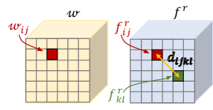
Here, we introduce a flexible objective that exploits global information about the reference features $f^{r}$, as discussed in Sec. 3.2. For convenience, we follow the convention for global correlation (1) by letting subscripts denote absolute spatial locations. When establishing matching confidences for a reference frame location $(i,j)$, the feature correlation layer $\mathbf{C}(f^{r},f^{q})$ only utilizes the encoded appearance $f^{r}_{ij}$ at the location $(i,j)$. However, the reference feature map $f^{r}$ also contains the encoding $f^{r}_{kl}$ of other image regions $(k,l)$, which are likely to also occur in the query $f^{q}$. To exploit this information, we therefore first replace the reference feature map $f^{r}$ with our filter map $w$. The aim is then to find $w$ which enforces high confidences $\mathbf{C}(w,f^{r})_{ijij}=w_{ij}^{\text{T}}f^{r}_{ij}\approx 1$ at the corresponding reference location $(i,j)$, while ensuring low matching confidences $\mathbf{C}(w,f^{r})_{ijkl}=w_{ij}^{\text{T}}f^{r}_{kl}\approx 0$ for other locations $(k,l)\neq(i,j)$ in the reference map $f^{r}$. These constraints aim at designing $w_{ij}$, that explicitly suppresses the corresponding matching confidences in regions $f^{r}_{kl}$ that have similar appearance as $f^{r}_{ij}$, since these regions may also occur in $f^{q}$.

As a first attempt, the aforementioned reference-frame constraints could be realized by minimizing the quadratic objective $\|\mathbf{C}(w,f^{r})-\delta\|^{2}$. Here, $\delta$ represents the desired correlation response, which in case of global correlation (1) is $\delta_{ijkl}=1$ whenever $(i,j)=(k,l)$ and $\delta_{ijkl}=0$ otherwise. The quadratic objective is attractive since it can be tackled with particularly effective optimization methods. On the other hand, the simple quadratic objective is known for its sensitivity to outliers. In our setting, the objective should in fact be largely indifferent to cases when a non-matching pair generates a strong negative correlation output $w_{ij}^{\text{T}}f^{r}_{kl}\ll 0$. This stems from the fact that any zero or negative confidence is enough to indicate a non-match. However, such strong negative predictions receive a disproportionately large impact in the quadratic objective, instead compromising the quality of the correspondence volume in challenging regions with similar appearance. This issue is further amplified by the severe imbalance between examples of matches and non-matches in the objective.

To address these issues, we formulate a robust non-linear least squares objective. For a non-matching location pair ($\delta_{ijkl}=0$), a positive correlation output $\mathbf{C}(w,f^{r})_{ijkl}>0$ corresponds to a similar appearance that should be suppressed, while negative correlation output $\mathbf{C}(w,f^{r})_{ijkl}<0$ is of little importance. We account for this asymmetry by introducing separate penalization weights $v^{\scriptscriptstyle+}_{ijkl}$ and $v^{\scriptscriptstyle-}_{ijkl}$ for positive and negative correlation outputs, respectively. The confidence values are thus mapped by the scalar function $\sigma$ defined as,

$$\sigma(c;v^{\scriptscriptstyle+}\!,v^{\scriptscriptstyle-}) =\begin{dcases}v^{\scriptscriptstyle+}c\,,&c\geq 0\\ v^{\scriptscriptstyle-}c\,,&c<0\end{dcases},\$$ (4a)

$$\sigma_{\eta}(c;v^{\scriptscriptstyle+}\!,v^{\scriptscriptstyle-}) =\frac{v^{\scriptscriptstyle+}\!-v^{\scriptscriptstyle-}\!}{2}\!\left(\!\sqrt{c^{2}+\eta^{2}}-\eta\right)+\frac{v^{\scriptscriptstyle+}\!+v^{\scriptscriptstyle-}\!}{2}c\,.$$ (4b)

We have also defined a smooth approximation $\sigma_{\eta}$, which for $\eta>0$ avoids the discontinuity in the derivative of $\sigma$ at $\mathbf{C}(w,f^{r})=0$. The original function $\sigma=\sigma_{0}$ is retrieved by setting $\eta=0$.

By applying the function (4), the confidence values $\mathbf{C}(w,f^{r})$ can be re-weighted using appropriate values for the weights $v^{\scriptscriptstyle+}$ and $v^{\scriptscriptstyle-}$. To address the question of how to set $v^{\scriptscriptstyle+}$ and $v^{\scriptscriptstyle-}$ in practice, recall that our objective defines a neural network module through the optimization (3). This opens an interesting opportunity of learning $v^{\scriptscriptstyle+}$ and $v^{\scriptscriptstyle-}$ as parameters of the neural network. These can thus be trained along with all other parameters of the network for the end task. Specifically, we parametrize the weights as functions $v^{\scriptscriptstyle+}_{ijkl}=v^{\scriptscriptstyle+}_{\theta}(d_{ijkl})$ and $v^{\scriptscriptstyle-}_{ijkl}=v^{\scriptscriptstyle-}_{\theta}(d_{ijkl})$ of the distance $d_{ijkl}=\sqrt{(i-k)^{2}+(j-l)^{2}}$ between $w_{ij}$ and the example $f^{r}_{kl}$. This strategy allows the network to learn the transition between the correct match $d_{ijij}=0$ and the distant $d_{ijkl}\gg 0$ examples of non-matching features $f^{r}_{kl}$. Our robust and learnable objective function for integrating reference frame information is thus formulated as,

$$L_{\text{r}}(w;f^{r},\theta)=\left\|\sigma_{\eta}\big{(}\mathbf{C}(w,f^{r});\,v^{\scriptscriptstyle+},v^{\scriptscriptstyle-}\big{)}-y\right\|^{2}\,.$$ (5)

Here we have additionally replaced the ideal correlation $\delta$ with a learnable target confidence $y_{ijkl}=y_{\theta}(d_{ijkl})$, to add further flexibility. We parametrize $v^{\scriptscriptstyle+}_{\theta}$, $v^{\scriptscriptstyle-}_{\theta}$, and $y_{\theta}$ using the strategy introduced in [5], as piece-wise linear functions of the distance $d_{ijkl}$, further detailed in the appendix Sec. C.

3.5 Query Frame Objective

In the previous section, we formulated an approach that integrates the reference feature map $f^{r}$ into the objective (3). However, as discussed in Sec. 3.2, there is also rich information to gain from the query frame. Firstly, correspondences between a pair of images must adhere to certain constraints, mainly that each point in the reference image can have at most a single match in the query image. Secondly, neighboring matches follow spatial smoothness priors, largely induced by the spatio-temporal continuity of the underlying 3D-scene. We encapsulate such constraints by defining a regularizing objective on the query frame,

$$L_{\text{q}}(w;\,f^{q},\theta)=\left\|R_{\theta}\ast\mathbf{C}(w,f^{q})\right\|^{2}\,.$$ (6)

Here, $\ast$ denotes the convolution operator and $R_{\theta}\in\mathbb{R}^{K^{4}\times Q}$ is a learnable 4D-kernel of spatial size $K$ and $Q$ number of output channels. A 4D-convolution operator allows us to fully utilize the structure of the 4D correspondence volume. Furthermore, its use is motivated by the translation invariance property induced by the 2D translation invariance of the two input feature maps. $R_{\theta}$ is learnt, along with all other network parameters, by the SGD-based minimization of the final network training loss.

The use of smoothness priors has a long and successful tradition in classic variational formulations for optical flow, developed during the pre-deep learning era [2, 7, 18, 37]. We therefore take inspiration from these ideas. However, our approach offers several interesting conceptual differences. First, our regularization operates directly on the matching confidences generated by the correlation operation, rather than the flow vectors. The correspondence volume provides a much richer description by encapsulating uncertainties in the correspondence assignment. Second, our objective is a function of the underlying filter map $w$, which is the input to the correlation layer. Third, our objective is implicitly minimized inside a deep neural network. Finally, this further allows our regularizer $R_{\theta}$ to be learned in a fully end-to-end and data-driven manner. In contrast, classical methods rely on hand-crafted regularizers and priors. By integrating information from a local 4D-neighborhood, the operator $R_{\theta}$ in (6) can enforce spatial smoothness by, for instance, learning differential operators. Moreover, our formulation lets the network learn the weighting of the query term (6) in relation to the reference frame objective (5), eliminating the need for such hyper-parameter tuning.

3.6 Filter map prediction module $P$

Our objective, employed in (3), is obtained by combining the reference (5) and query (6) terms as,

$$L(w;f^{r},f^{q},\theta)=L_{\text{r}}(w;f^{r},\theta)+L_{\text{q}}(w;\,f^{q},\theta)+\|\lambda_{\theta}w\|^{2}\,.$$ (7)

The last term corresponds to a regularizing prior on $w$, weighted by the learnable scalar $\lambda_{\theta}\in\mathbb{R}$. Note that while the reference frame objective $L_{\text{r}}$ in (5) can be decomposed into independent terms for each location $w_{ij}$, the query term $L_{\text{q}}$ (6) introduces dependencies between all elements in $w$. Efficiently optimizing such a high-dimensional problem during the forward pass of the network in order to implement (3) may seem an impossibility. Next, we demonstrate that this can, in fact, be achieved by a combination of accurate initialization and a simple but powerful iterative procedure. Any neural network architecture employing feature correlation layers can thereby benefit from our module.

Optimizer: While finding the global optima of (7) within a small tolerance is costly, this is not necessary in our case. Instead, we can effectively utilize the information encoded in the objective (7) by optimizing it to a sufficient degree. We therefore derive the filter map $w^{*}=P_{\theta}(f^{r},f^{q})$ by applying an iterative optimization strategy. Specifically, we use the Steepest Descent algorithm, which was found effective in [5]. Given the current iterate $w^{n}$, the steepest descent method [41, 53] finds the step-length $\alpha^{n}$ that minimizes the objective in the gradient direction. This is obtained through a simple closed-form expression by first performing a Gauss-Newton approximation of (5). The filter map is then updated by taking a gradient step with optimal length $\alpha^{n}$,

$$w^{n+1}=w^{n}-\alpha^{n}\nabla L\left(w^{n};f^{r},f^{q},\theta\right)\,,\quad\alpha^{n}=\operatorname*{arg\,min}_{\alpha}L_{\text{GN}}^{n}\big{(}w^{n}-\alpha\nabla L(w^{n};f^{r},f^{q},\theta)\big{)}\,.$$ (8)

Here, $L_{\text{GN}}^{n}$ is the Gauss-Newton approximation of (7) at $w^{n}$. Both the gradient $\nabla L$ and the step length $\alpha^{n}$ are implemented using their closed form expressions with standard neural network modules, as detailed in the appendix Sec. A. Importantly, the operation (8) is fully differentiable w.r.t. $f^{r}$, $f^{q}$, and $\theta$, allowing end-to-end training of all underlying network parameters.

Initializer: To reduce the number of optimization iterations needed in the filter predictor network $P$, we generate an initial filter map $w^{0}$ using an efficient and learnable module. We parametrize $w^{0}_{ij}=a_{ij}f^{r}_{ij}+b_{ij}\bar{f^{r}}$, where $\bar{f^{r}}\in\mathbb{R}^{d}$ is the spatial average reference vector, encoding contextual information. Intuitively, we wish $w^{0}$ to have a high activation $(w^{0}_{ij})^{\text{T}}f^{r}_{ij}=1$ at the matching position and $(w^{0}_{ij})^{\text{T}}\bar{f^{r}}=0$. The scalar coefficients $a_{ij}$ and $b_{ij}$ are then easily found by solving these equations. Details are given in the appendix Sec. B.

4 Experiments

We perform comprehensive experiments for two tasks: geometric correspondences and optical flow. We additionally show that our method can be successfully applied to the task of semantic matching. Both global and local correlation-based versions of our GOCor module are analyzed by integrating them into two recent state-of-the-art networks. Further results, analysis, and visualizations along with more details regarding architectures and datasets are provided in the appendix.

4.1 Geometric matching

We first evaluate our GOCor module for dense geometric matching by integrating it into the recent GLU-Net [59]. GLU-Net is a 4-level pyramidal network, operating at two image resolutions to estimate dense flow fields. It relies on a global correlation at the coarsest level to capture long-range displacements and uses local correlations in the subsequent levels.

Experimental setup: We create GLU-Net-GOCor by replacing global and local feature correlation layers with our global and local GOCor modules, respectively. The global GOCor module employs the full objective (7), while the local variant uses only the reference term (5). We use three steepest descent iterations during training and increase the number during inference. We follow the same self-supervised training procedure and data as in [59], applying synthetic homography transformations to images compiled from different sources to ensure diversity. We refer to this as the Static dataset, since it simulates a static scene. For better compatibility with real 3D scenes and moving objects, we further introduce a Dynamic training dataset, by augmenting the Static data with random independently moving objects from the COCO [36] dataset. In all experiments, we compare the results of GLU-Net and GLU-Net-GOCor trained with the same data, and according to the same procedure.

Evaluation datasets and metrics: We first employ the 59 sequences of the HPatches dataset [3], consisting of planar scenes from different viewpoints. We additionally utilize the multi-view ETH3D dataset [51], depicting indoor and outdoor scenes captured from a moving hand-held camera. We follow the protocol of [59], sampling image pairs at different intervals to analyze varying magnitude of geometric transformations. Finally, because of the difficulty to obtain dense annotations on real imagery with extreme viewpoint and varying imaging condition, we also evaluate our model on sparse correspondences available on the MegaDepth [34] dataset, according to the protocol introduced in [52]. We use the Static training data for the comparison on the HPatches dataset and the Dynamic training data for the ETH3D and MegaDepth datasets. In line with previous works [39, 59], we employ the Average End-Point Error (AEPE) and Percentage of Correct Keypoints at a given pixel threshold $T$ (PCK-$T$) as the evaluation metrics.

Table 1: HPatches homography dataset [3].

	AEPE $\downarrow$	PCK-1 (%) $\uparrow$	PCK-5 (%) $\uparrow$
DGC-Net [39]	33.26	12.00	58.06
GLU-Net	25.05	39.55	78.54
GLU-Net-GOCor (Ours)	20.16	41.55	81.43

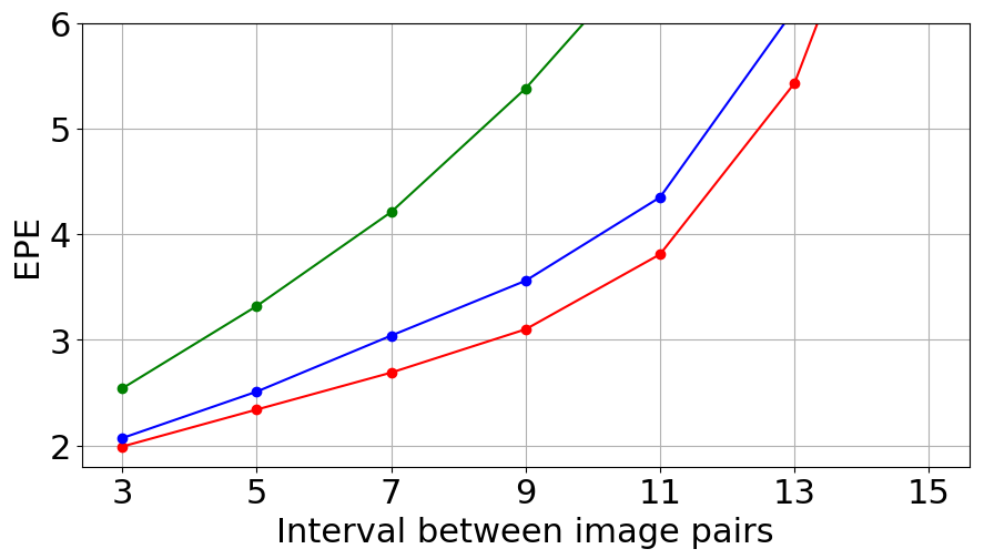
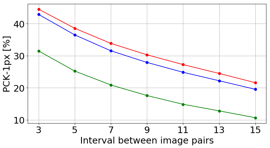
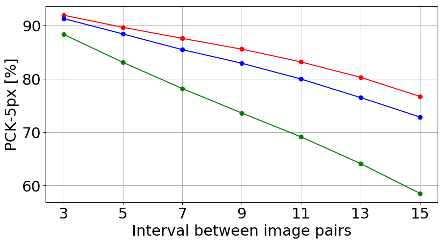
Results: In Table 1, we present results on HPatches. We also report the results of the recent state-of-the-art DGC-Net [39] for reference. Our GLU-Net-GOCor outperforms original GLU-Net by a large margin, achieving both higher accuracy in terms of PCK, and better robustness to large errors as indicated by AEPE. In Figure 4, we plot AEPE, PCK-1 and PCK-5 obtained on the ETH3D images. For all intervals, our approach is consistently better than baseline GLU-Net. We note that the improvement is particularly prominent at larger intra-frame intervals, strongly indicating that our GOCor module better copes with large appearance variations due to large viewpoint changes, compared to the feature correlation layer.

Table 2: Results on sparse correspondences of the MegaDepth dataset [34].

	PCK-1 (%) $\uparrow$	PCK-3 (%) $\uparrow$	PCK-5 (%) $\uparrow$
GLU-Net	21.58	52.18	61.78
GLU-Net-GOCor (Ours)	37.28	61.18	68.08

This is also confirmed by the results on MegaDepth in Table 2. Images depict extreme view-point changes with as little as 10% of co-visible regions. In this case as well, GOCor brings significant improvement, particularly in pixel-accuracy (PCK-1).

Figure 4: Results on geometric matching dataset ETH3D [51]. AEPE (left), PCK-1 (center), and PCK-5 (right) are plotted w.r.t. the inter-frame interval length.

4.2 Optical flow

Next, we evaluate our GOCor module for the task of optical flow estimation, by integrating it into the state-of-the-art PWC-Net [55, 56] and GLU-Net [59] architectures. PWC-Net [55] is based on a 5-level pyramidal network, estimating the dense flow field at each level using a local correlation layer.

Experimental setup: We replace all local correlation layers with our local GOCor module to obtain PWC-Net-GOCor. We finetune PWC-Net-GOCor on 3D-Things [24], using the publicly available PWC-Net weights trained on Flying-Chairs [16] and 3D-Things [24] as initialization. For fair comparison, we also finetune the standard PWC-Net on 3D-Things with the same schedule. Finally, we also finetune PWC-Net-GOCor on the Sintel [8] training dataset according to the schedule introduced in [24, 55]. As described in Sec. 4.1, we train both GLU-Net and GLU-Net-GOCor on the Dynamic training set. For the global and local GOCor modules, we use the same settings as in 4.1.

Datasets and evaluation metrics: For evaluation, we use the established KITTI dataset [17], composed of real road sequences captured by a car-mounted stereo camera rig. We also utilize the Sintel dataset [8], which consists of 3D animated sequences. We use the standard evaluation metrics, namely the AEPE and F1 for KITTI. The latter represents the percentage of optical flow outliers. For Sintel, we employ AEPE together with PCK, i.e. percentage of inliers. In line with [21, 22, 55, 56, 59], we show results on the training splits of these datasets.

Table 3: Results for the optical flow task on the training splits of KITTI [17] and Sintel [8]. A result in parenthesis indicates that the dataset was used for training.

	KITTI-2012		KITTI-2015		Sintel Clean			Sintel Final
	AEPE $\downarrow$	F1 (%) $\downarrow$	AEPE $\downarrow$	F1 (%) $\downarrow$	AEPE $\downarrow$	PCK-1 (%) $\uparrow$	PCK-5 (%) $\uparrow$	AEPE $\downarrow$	PCK-1 (%) $\uparrow$	PCK-5 (%) $\uparrow$
GLU-Net	3.14	19.76	7.49	33.83	4.25	62.08	88.40	5.50	57.85	85.10
GLU-Net-GOCor	2.68	15.43	6.68	27.57	3.80	67.12	90.41	4.90	63.38	87.69
PWC-Net (from paper)	4.14	21.38	10.35	33.67	2.55	-	-	3.93	-	-
PWC-Net (ft 3D-Things)	4.34	20.90	10.81	32.75	2.43	81.28	93.74	3.77	76.53	90.87
PWC-Net-GOCor (ft 3D-Things)	4.12	19.31	10.33	30.53	2.38	82.17	94.13	3.70	77.34	91.20
PWC-Net (ft Sintel)	2.94	12.70	8.15	24.35	(1.70)	-	-	(2.21)	-	-
PWC-Net-GOCor (ft Sintel)	2.60	9.67	7.64	20.93	(1.74)	(87.93)	(95.54)	(2.28)	(84.15)	(93.71)

Results: Results are reported in Tab. 3. First, compared to the GLU-Net baseline, our GOCor module brings significant improvements in both AEPE and F1/PCK on all optical flow datasets. Next we compare the PWC-Net based methods trained on 3D-Things (middle section) and report the official result [55, 56] along with our fine-tuned versions. While our PWC-Net-GOCor obtains a similar AEPE, it achieves substantially better accuracy, with a $3\%$ improvement in F1 metric on KITTI-2015. After finetuning on Sintel images, both PWC-Net and PWC-Net-GOCor achieve similar results on the Sintel training data (in parenthesis). However, the PWC-Net-GOCor version provides superior results on the two KITTI datasets. This clearly demonstrates the superior domain generalization capabilities of our GOCor module. Note that both methods in the bottom section of Tab. 3 are only trained on animated datasets, while KITTI consists of natural road-scenes. Thanks to the effective objective-based adaption performed in our matching module during inference, PWC-Net-GOCor excels even with a sub-optimal feature embedding trained for animated images, and when exposed to previously unseen motion patterns. This is a particularly important property in the context of optical flow and geometric matching, where collection of labelled realistic training data is prohibitively expensive, forcing methods to resort to synthetic and animated datasets.

4.3 Generalization to semantic matching

Table 4: PCK [%] on TSS [58].

	FGD3Car	JODS	PASCAL	All
Semantic-GLU-Net [59]	94.4	75.5	78.3	82.8
GLU-Net	93.2	73.3	71.1	79.2
GLU-Net-GOCor (Ours)	94.6	77.9	77.7	83.4

We additionally compare the performance of GOCor to the feature correlation layer on the task of semantic matching. In Table 4, we evaluate our GLU-Net-GOCor trained on the Static data without any additional finetuning, for dense semantic matching on the TSS dataset [58]. In the semantic correspondence task, images depict different instances of the same object category (e.g. horse). As a result, the value of additional reference frame information (Sec. 3.2 and  3.4) is not as pronounced in semantic matching compared to geometric matching or optical flow. Indeed, our reference frame objective uses its full potential when both the reference and the query images depict similar regions from the same scene. Nevertheless, our GLU-Net-GOCor sets a new state-of-the-art on this dataset, even outperforming Semantic-GLU-Net [59].

4.4 Run-time

Table 5: Run time [ms] averaged over the 194 image pairs of KITTI-2012.

	Run-time [ms]
PWC-Net	118.05
PWC-Net-GOCor	203.02
GLU-Net	154.97
GLU-Net-GOCor	261.90

In Table 5, we compare the run time of our GOCor-based networks to their original versions on the KITTI-2012 dataset. The timings are obtained on the same desktop with an NVIDIA Titan X GPU. While our GOCor module leads to increased computation, the run-time remains within reasonable margins thanks to our dedicated optimization module, described in Sec. 3.6. We can further control the trade of between computation and performance by varying the number of steepest descent iterations in our GOCor module. In Appendix E.1 we provide such a detailed analysis, and propose faster operating points with only minor degradation in performance.

Table 6: Ablation study of key aspects of our approach on three different datasets.

		HPatches		KITTI-2012		KITTI-2015
		AEPE $\downarrow$	PCK-5 (%) $\uparrow$	AEPE $\downarrow$	F1 (%) $\downarrow$	AEPE $\downarrow$	F1 (%) $\downarrow$
(I)	BaseNet	30.94	69.22	4.03	30.49	8.93	48.66
(II)	BaseNet + NC-Net [47]	39.15	63.52	4.41	34.78	9.86	52.78
(III)	BaseNet + Global-GOCor Linear Regression	27.02	68.12	4.31	35.30	8.93	52.64
(IV)	BaseNet + Global-GOCor $L_{\text{r}}$	26.27	71.29	3.91	29.77	8.50	46.24
(V)	BaseNet + Global-GOCor $L_{\text{r}}+L_{\text{q}}$	25.30	71.21	3.74	26.82	7.87	43.08
(VI)	BaseNet + Global-GOCor $L_{\text{r}}+L_{\text{q}}$ + Local-GOCor	23.57	78.30	3.45	25.42	7.10	39.57

Figure 5: Visualization of the matching confidences computed between the indicated location (green) in the reference image and all locations of either the reference image itself or the query image.

4.5 Ablation study

Finally, we analyze key components of our approach. We first design a powerful baseline architecture estimating dense flow fields, called BaseNet. It consists of a three-level pyramidal CNN-network, inspired by [59], employing a global correlation layer followed by two local layers. All methods are trained with the Dynamic data, described in Sec. 4.1. Results on HPatches, KITTI-2012 and KITTI-2015 are reported in Tab. 6. We first analyse the effect of replacing the feature correlation layer with GOCor at the global correlation level. The version denoted (IV) employs our global GOCor using solely the reference-based objective $L_{\text{r}}$ (Sec. 3.4). It leads to significantly better results on all datasets compared to standard BaseNet (I). Instead of our robust reference loss $L_{\text{r}}$, the version (III) employs a standard linear regression objective $\|\mathbf{C}(w,f^{r})-\delta\|^{2}$, leading to substantially worse results. We also compare with adding the post-processing strategy proposed in [47] (II), employing 4D-convolutions and enforcing cyclic consistency. This generally leads to a degradation in performance, likely caused by the inability to cope with the domain gap between training and test data. From (IV) to (V) we integrate our query frame objective $L_{\text{q}}$ (Sec. 3.5), which results in major gains, particularly on the more challenging KITTI datasets. Finally, we replace the local correlation layers with our local GOCor module in (VI). This leads to large improvements on all datasets and metrics.

In Figure 5, we visualize the relevance of our reference loss (Sec. 3.4) qualitatively by plotting the correspondence volume outputted by our global GOCor module, when correlating a particular point (i,j) of the reference image with all locations of either the reference itself or the query image. The predicted correspondence volume gets increasingly distinctive after each iteration in the GOCor layer. Specifically, it is clearly visible that final matching confidences with the query image benefits from optimizing the correlation scores with the reference image itself, using Eq. (5).

5 Conclusion

We propose a neural network module for predicting globally optimized matching confidences between two deep feature maps. It acts as a direct alternative to feature correlation layers. We integrate unexploited information about the reference and query frames by formulating an objective function, which is minimized during inference through an iterative optimization strategy. Our approach thereby explicitly accounts for, e.g., similar image regions. Our resulting GOCor module is thoroughly analysed and evaluated on the tasks of geometric correspondences and optical flow, with an extension to dense semantic matching. When integrated into state-of-the-art networks, it significantly outperforms the feature correlation layer.

Broader Impact

Our feature correspondence matching module can be beneficial in a wide range of applications relying on explicit or implicit matching between images, such as visual localization [50, 57], 3D-reconstruction [1], structure-from-motion [49], action recognition [54] and autonomous driving [25]. On the other hand, any image matching algorithm runs the risk of being used for malevolent tasks, such as malicious image manipulation or image surveillance system. However, our module is only one building block to be integrated in a larger pipeline. On its own, it therefore has little chances of being wrongfully used.

Appendix

In this appendix, we first provide the details of the derivation of the filter map $w^{*}$ within the filter map predictor module $P$ in Section A. We then give the expression for the initial estimate $w^{0}$ in Section B. In Section C, we provide further insights on the architecture of our GOCor module as well as the implementation details. In Section D, we give more details about the evaluation datasets, metrics and networks utilized. We then provide additional quantitative and qualitative results of our approach GOCor compared to the feature correlation layer in Section E. Finally, we further analyse our approach in an extended ablation study in Section F.

Appendix A Derivation of filter map prediction module $P$

Here, we derive the iterative updates employed in our module $P_{\theta}$, which aims to solve $w^{*}=P_{\theta}(f^{r},f^{q})=\operatorname*{arg\,min}_{w}L(w;f^{r},f^{q},\theta)$ (Eq. 3). Our final objective (Eqs. 5-7) is given by,

$$L(w;f^{r},f^{q},\theta) =L_{\text{r}}(w;f^{r},\theta)+L_{\text{q}}(w;f^{q},\theta)+\|\lambda_{\theta}w\|^{2}$$ (9a)

$$L_{\text{r}}(w;f^{r},\theta) =\left\|\sigma_{\eta}\big{(}\mathbf{C}(w,f^{r});\,v^{\scriptscriptstyle+},v^{\scriptscriptstyle-}\big{)}-y\right\|^{2}$$ (9b)

$$L_{\text{q}}(w;f^{q},\theta) =\left\|R_{\theta}\ast\mathbf{C}(w,f^{q})\right\|^{2}\,.$$ (9c)

As discussed in Sec. 3.6, we do not need to attain a global optimum. The goal is to significantly minimize the loss $L$, using only a few iterations for efficiency. To this end we employ the Steepest Descent methodology [41, 53]. In the steepest descent algorithm, we update the parameters by taking steps $w^{n+1}=w^{n}-\alpha^{n}\nabla L\left(w^{n}\right)$ in the gradient direction $\nabla L\left(w^{n}\right)$ with step length $\alpha^{n}$. The aim is to find the step length $\alpha^{n}$ that leads to a maximal decrease in the objective. This is performed by first approximating the loss with a quadratic function at the current estimate $w^{n}$,

$$L(w)\approx L^{n}_{\text{GN}}(w)=\frac{1}{2}\left(w-w^{n}\right)^{\mathrm{T}}Q^{n}\left(w-w^{n}\right)+\left(w-w^{n}\right)^{\mathrm{T}}\nabla L\left(w^{n}\right)+L\left(w^{n}\right)$$ (10)

Here, we see $w^{n}$ as a vector. We set the Hermitian positive definite matrix $Q^{n}$ according to the Gauss-Newton method [41] $Q^{n}=(J^{n})^{\text{T}}J^{n}$, where $J^{n}$ is the Jacobian of the residual at $w^{n}$. To avoid clutter, the dependence on $f^{r},f^{q},\theta$ is made implicit. In the rest of the section, unless otherwise stated, matrices multiplications are element-wise.

The steepest descent method [41, 53] finds the step-length $\alpha^{n}$ that minimizes the loss (10) in the gradient direction. Due to the convexity of (10), this is obtained by solving $\frac{\mathrm{d}}{\mathrm{d}\alpha}L_{\text{GN}}\left(w^{n}-\alpha\nabla L\left(w^{n}\right)\right)=0$, which leads to the expression,

$$\alpha^{n}=\frac{\nabla L\left(w^{n}\right)^{\mathrm{T}}\nabla L\left(w^{n}\right)}{\nabla L\left(w^{n}\right)^{\mathrm{T}}Q^{n}\nabla L\left(w^{n}\right)}=\frac{\left\|\nabla L\left(w^{n}\right)\right\|^{2}}{\left\|J^{n}\nabla L\left(w^{n}\right)\right\|^{2}}$$ (11)

In the next subsections, we derive the expression for $\nabla L$ and subsequently for step-length $\alpha$.

A.1 Closed form expression of $\nabla L$

Here, we derive a closed-form expression for the gradient of the loss (9a). The gradient $\nabla L(w)$ of the loss (9a) with respect to the filters $w$ is then computed as,

$$\nabla L(w)=\nabla L_{\text{r}}(w)+\nabla L_{\text{q}}(w)+2\lambda_{\theta}^{2}w\,.$$ (12)

Expression of $\nabla L_{\text{r}}(w)$: $L_{\text{r}}$ is defined according to (9b) and equation (5) of the main paper, such as $L_{r}=\left\|r_{r}(w,f^{r})\right\|^{2}$. Here, $r_{r}$ designates the residual function, which is formulated as (also Eq. 4),

$$r_{r}(w,f^{r})= \,\sigma_{\eta}\big{(}\mathbf{C}(w,f^{r});\,v^{\scriptscriptstyle+},v^{\scriptscriptstyle-}\big{)}-y$$ (13)

$$\sigma_{\eta}\big{(}\mathbf{C}(w,f^{r});\,v^{\scriptscriptstyle+},v^{\scriptscriptstyle-}\big{)}= \,\frac{v^{\scriptscriptstyle+}-v^{\scriptscriptstyle-}}{2}\!\left(\!\sqrt{\mathbf{C}(w,f^{r})^{2}+\eta^{2}}-\eta\right)+\frac{v^{\scriptscriptstyle+}+v^{\scriptscriptstyle-}}{2}\mathbf{C}(w,f^{r})\,.$$ (14)

The gradient of $\nabla L_{\text{r}}(w)$ of the loss (9b) w.r.t $w$ is given by:

$$\nabla L_{\text{r}}(w)=2\left[\frac{\partial r_{r}(w,f^{r})}{\partial w}\right]^{\text{T}}r_{r}(w,f^{r})$$ (15)

where $J_{r}=\frac{\partial r_{r}(w,f^{r})}{\partial w}$ corresponds to the Jacobian of the residual function (13) with respect to filters w. Using the chain rule we obtain,

$$J_{r}=\frac{\partial r_{r}(w,f^{r})}{\partial w}=\frac{\partial\sigma_{\eta}}{\partial\mathbf{C}(w,f^{r})}\frac{\partial\mathbf{C}(w,f^{r})}{\partial w}\,,$$ (16)

Using (14), the derivative of the error function is obtained as

$$\frac{\partial\sigma_{\eta}}{\partial\mathbf{C}(w,f^{r})}=\left[\frac{v^{\scriptscriptstyle+}-v^{\scriptscriptstyle-}}{2}\left(\frac{\mathbf{C}(w,f^{r})}{\sqrt{\mathbf{C}(w,f^{r})^{2}+\eta^{2}}}\right)+\frac{v^{\scriptscriptstyle+}+v^{\scriptscriptstyle-}}{2}\right]\,.$$ (17)

Integrating (16) into (15) leads to the final formulation of $\nabla L_{\text{r}}(w)$ as

$$\nabla L_{\text{r}}(w)=2\left[\frac{\partial\mathbf{C}(w,f^{r})}{\partial w}\right]^{\text{T}}\left[\left(\frac{v^{\scriptscriptstyle+}-v^{\scriptscriptstyle-}}{2}\left(\frac{\mathbf{C}(w,f^{r})-y}{\sqrt{(\mathbf{C}(w,f^{r})-y)^{2}+\eta^{2}}}\right)+\frac{v^{\scriptscriptstyle+}+v^{\scriptscriptstyle-}}{2}\right)r_{r}(w,f^{r})\right]\,.$$ (18)

The multiplication with the transposed Jacobian $\left[\frac{\partial\mathbf{C}(w,f^{r})}{\partial w}\right]^{\text{T}}$ corresponds to back-propagation through the correlation layer $\mathbf{C}$. This can be efficiently implemented with standard operations.

Expression of $\nabla L_{\text{q}}$: The loss on the query frame $L_{\text{q}}$ is formulated in (9c) and in eq. 6 of the main paper, as $L_{\text{q}}(w)=\left\|r_{q}(w,f^{q})\right\|^{2}$, where the residual $r_{q}$ is defined below:

$$r_{q}(w,f^{q})=R_{\theta}\ast\mathbf{C}(w,f^{q})$$ (19)

Following similar steps than for $L_{\text{r}}$, the gradient $\nabla L_{\text{q}}$ of the loss (9c) w.r.t. the filters $w$ is then computed as,

$$\nabla L_{\text{q}}=2\left[\frac{\partial r_{q}(w,f^{q})}{\partial w}\right]^{\text{T}}r_{q}(w,f^{q})$$ (20)

where $J_{q}=\frac{\partial r_{q}(w,f^{q})}{\partial w}$ corresponds to the Jacobian of the residual function (19) with respect to the filter map $w$.

$$J_{q}=R_{\theta}\ast\frac{\partial\mathbf{C}(w,f^{q})}{\partial w}\,.$$ (21)

This leads to the final formulation of the gradient as,

$$\nabla L_{\text{q}}=2\left[\frac{\partial\mathbf{C}(w,f^{q})}{\partial w}\right]^{\text{T}}\left[R_{\theta}\ast\right]^{\text{T}}r_{q}(w,f^{q})\,.$$ (22)

Here, $\left[R_{\theta}\ast\right]^{\text{T}}$ denotes the transposed convolution with the kernel $R_{\theta}$.

A.2 Calculation of step-length $\alpha^{n}$

In this section, we show the calculation of the denominator of $\alpha^{n}=\frac{\alpha^{n}_{\text{num}}}{\alpha^{n}_{\text{den}}}$. The denominator in equation (11) is given by,

$$\alpha^{n}_{\text{den}}= \left\|J^{n}\nabla L\left(w^{n}\right)\right\|^{2}$$ (23)

$$= \left\|\left.J_{r}(w)\right|_{w^{n}}\nabla L\left(w^{n}\right)\right\|^{2}+\left\|\left.J_{q}(w)\right|_{w^{n}}\nabla L\left(w^{n}\right)\right\|^{2}+\left\|\lambda_{\theta}\nabla L\left(w^{n}\right)\right\|^{2}$$

Using equations (16) and (21), we finally obtain:

$$\alpha^{n}_{\text{den}}= \,\left\|\left.\ \frac{\partial\sigma_{\eta}}{\partial\mathbf{C}(w,f^{r})}\frac{\partial\mathbf{C}(w,f^{r})}{\partial w}\right|_{w^{n}}\nabla L\left(w^{n}\right)\right\|^{2}+\left\|\left.R_{\theta}\ast\frac{\partial\mathbf{C}(w,f^{q})}{\partial w}\right|_{w^{n}}\nabla L\left(w^{n}\right)\right\|^{2}+\left\|\lambda_{\theta}\nabla L\left(w^{n}\right)\right\|^{2}$$

$$= \,\left\|\frac{\partial\sigma_{\eta}}{\partial\mathbf{C}(w,f^{r})}\mathbf{C}(\nabla L\left(w^{n}\right),f^{r})\right\|^{2}+\left\|R_{\theta}\ast\mathbf{C}(\nabla L\left(w^{n}\right),f^{q})\right\|^{2}+\left\|\lambda_{\theta}\nabla L\left(w^{n}\right)\right\|^{2}$$ (24)

The relation $\left.\frac{\partial\mathbf{C}(w,f^{r})}{\partial w}\right|_{w^{n}}\nabla L\left(w^{n}\right)=\mathbf{C}(\nabla L\left(w^{n}\right),f^{r})$ stems from the linearity of $\mathbf{C}$ in the first argument. All operations in (A.2) can thus easily be implemented using standard neural network operations. We summarize the different steps taking place within the filter map predictor module $P$ in algorithm 1.

Algorithm 1 Filter Predictor module $P$.

1:Reference and Query feature maps $f^{r},f^{q}$, iterations $N_{\text{iter}}$

2:$w^{0}\leftarrow\mathtt{ModelInit}(f^{r})$        # Initialize filter map (sec. 3.6 of main paper)

3:for $i=0,\ldots,N_{\text{iter}}-1$ do        # Optimizer module loop

4:     $\nabla L(w^{n})\leftarrow\mathtt{FiltGrad}(w^{n},f^{r},f^{q})$    # Using (18) - (22)

5:     $\alpha^{n}_{\text{num}}\leftarrow\left\|\nabla L\left(w^{n}\right)\right\|^{2}$

6:     $\alpha^{n}_{\text{den}}\leftarrow\left\|J^{n}\nabla L\left(w^{n}\right)\right\|^{2}$             # Apply Jacobian (16) and (21)

7:     $\alpha^{n}\leftarrow\alpha^{n}_{\text{num}}/\alpha^{n}_{\text{den}}$      # Compute step length (11)

8:     $w^{n+1}\leftarrow w^{n}-\alpha^{n}\nabla L(w^{n})$      # Update filter map

9:end for

Appendix B Initial estimate of $w^{0}$

As explained in Section 3.6 of the main paper, to reduce the number of optimization iterations needed in the filter predictor network $P$, we generate an initial filter map $w^{0}$, which is then processed by the optimizer module to provide the final discriminative filter $w^{*}=P(f^{r},f^{q})$.

We wish that $w^{0}$ integrates information about the entire reference feature map $f^{r}$. We thus formulate $w^{0}$ at location $(i,j)$ as a linear combination of $f^{r}_{ij}$ and $\bar{f^{r}}$, where $\bar{f^{r}}\in\mathbb{R}^{D}$ is the spatial average reference vector, encoding contextual information. We obtain $w^{0}$ by solving for the scalar factors $a_{ij},b_{ij}$ that adhere to the following constraints,

$$w^{0}_{ij}=a_{ij}f^{r}_{ij}+b_{ij}\bar{f^{r}}$$ (25a)

$$(w^{0}_{ij})^{\text{T}}f^{r}_{ij}=\beta$$ (25b)

$$(w^{0}_{ij})^{\text{T}}\bar{f^{r}}=\gamma$$ (25c)

In the simplest setting, $\beta$ can be set to one and $\gamma$ to zero. However, we let these values be learnt from data. The scalar coefficients $a_{ij}$ and $b_{ij}$ are then easily found by solving these equations, resulting in the following formulation for $w^{0}$,

$$w^{0}_{ij}=\frac{\left[\beta\left\|\bar{f^{r}}\right\|^{2}-\gamma(f^{r}_{ij})^{\text{T}}\bar{f^{r}}\right]f^{r}_{ij}-\left[\beta(f^{r}_{ij})^{\text{T}}\bar{f^{r}}-\gamma\left\|f^{r}_{ij}\right\|^{2}\right]\bar{f^{r}}}{\left\|\bar{f^{r}}\right\|^{2}\left\|f^{r}_{ij}\right\|^{2}-\left((f^{r}_{ij})^{\text{T}}\bar{f^{r}}\right)^{2}}$$ (26)

As already mentioned, $\beta$ and $\gamma$ are learnable weights. In the simplest case, both are just scalars. We call this version ContextAwareInitializer. To add further flexibility, they can alternatively be vectors of the same dimension $D$ than the reference feature map $f^{r}\in\mathbb{R}^{H\times W\times D}$, such that $\beta,\gamma\in\mathbb{R}^{D}$. We refer to this variant of the initializer as Flexible-ContextAwareInitializer. Both versions explicitly integrate context information about the entire reference feature map.

We additionally define a simpler alternative for $w^{0}$, that we call SimpleInitializer for which it is assumed that $(f^{r}_{ij})^{\text{T}}\bar{f^{r}}=0$. As a result, $w_{ij}$ only depends on the reference feature $f^{r}_{ij}$ at this location, $w^{0}$ can thus be formulated as:

$$w^{0}_{ij}=\beta\frac{f^{r}_{ij}}{\left\|f^{r}_{ij}\right\|}$$ (27)

Here, $\beta$ can also be either a scalar (SimpleInitializer) or a vector of dimension $D$ (Flexible-SimpleInitializer).

In our Global-GOCor module, we use the variant Flexible-ContextAwareInitializer for our initializer module. We defend this choice in our supplementary ablation study Section F. For our Local-GOCor module, we instead use the SimpleInitializer variant of the initializer.

Appendix C Architecture details

Expression for $y,v^{\scriptscriptstyle-},v^{\scriptscriptstyle+}$: Here we discuss the parametrization of $y,v^{\scriptscriptstyle-},v^{\scriptscriptstyle+}$, introduced in the reference loss formulation in Sec. 3.4.

For the implementation, we define $y=v^{\scriptscriptstyle+}y^{\prime}$ and $v^{\scriptscriptstyle-}=v^{\scriptscriptstyle+}m$, with element-wise multiplication. We parametrize $y^{\prime},v^{\scriptscriptstyle+},m$ as functions of the distance $d_{ijkl}=\sqrt{(i-k)^{2}+(j-l)^{2}}$ between $w_{ij}$ and the example $f^{r}_{kl}$, such that $y^{\prime}_{ijkl}=y^{\prime}_{\theta}(d_{ijkl}),\,v^{\scriptscriptstyle+}_{ijkl}=v^{\scriptscriptstyle+}_{\theta}(d_{ijkl}),\,m_{ijkl}=m_{\theta}(d_{ijkl})$.

All three are expressed with triangular basis function, as in [5]. For example, the function $v^{\scriptscriptstyle+}$ at position $(i,j,k,l)$ is given by:

$$v^{\scriptscriptstyle+}_{ijkl}=\sum_{k=0}^{N-1}(v^{\scriptscriptstyle+}_{\theta})^{k}\rho_{k}(d_{ijkl})$$ (28)

with triangular basis functions $\rho_{k}$, expressed as

$$\rho_{k}(d)=\left\{\begin{array}[]{ll}\max\left(0,1-\frac{|d-k\Delta|}{\Delta}\right),&k<N-1\\ \max\left(0,\min\left(1,1+\frac{d-k\Delta}{\Delta}\right)\right),&k=N-1\end{array}\right.$$ (29)

We use $N=10$ basis functions and set the knot displacement to $\Delta=0.5$ in the resolution of the deep feature space. The final case $k=N-1$ represents all locations $(k,l)$ that are far away from $(i,j)$ and thus can be treated identically.

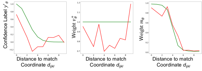
The coefficients $y^{\prime}_{\theta},v^{\scriptscriptstyle+}_{\theta},m_{\theta}$ are learnt from data, as part of the filter predictor module $P$. For $m$, we constrain the values in the interval $\left[0,1\right]$ by passing the output of (28) through a Sigmoid function. We initialize the target confidence $y^{\prime}_{\theta}$ to a Gaussian, with mean equal to 0 and standard deviation equal to 1. The positive weight function $v^{\scriptscriptstyle+}_{\theta}$ is initialized to a constant so that $v^{\scriptscriptstyle+}_{ijkl}=1$ while we initialize the function $m_{\theta}$ with a scaled tanh function.

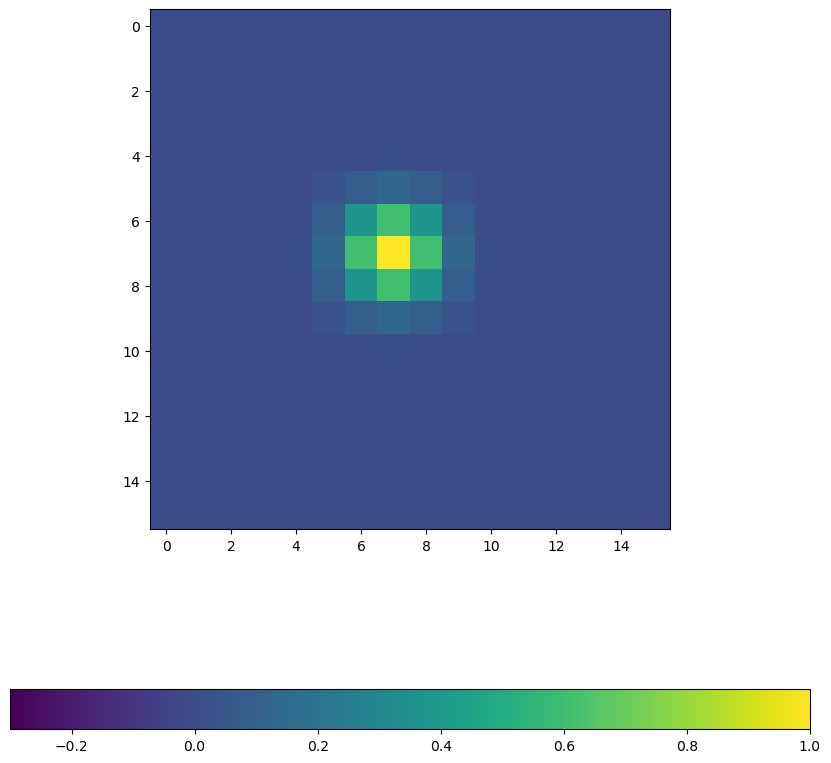
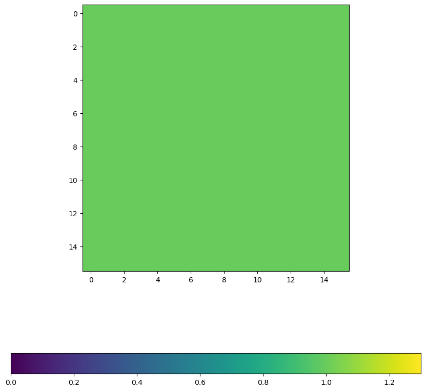
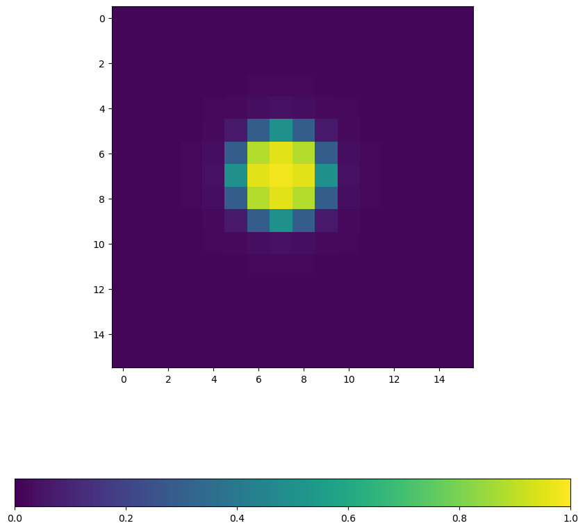
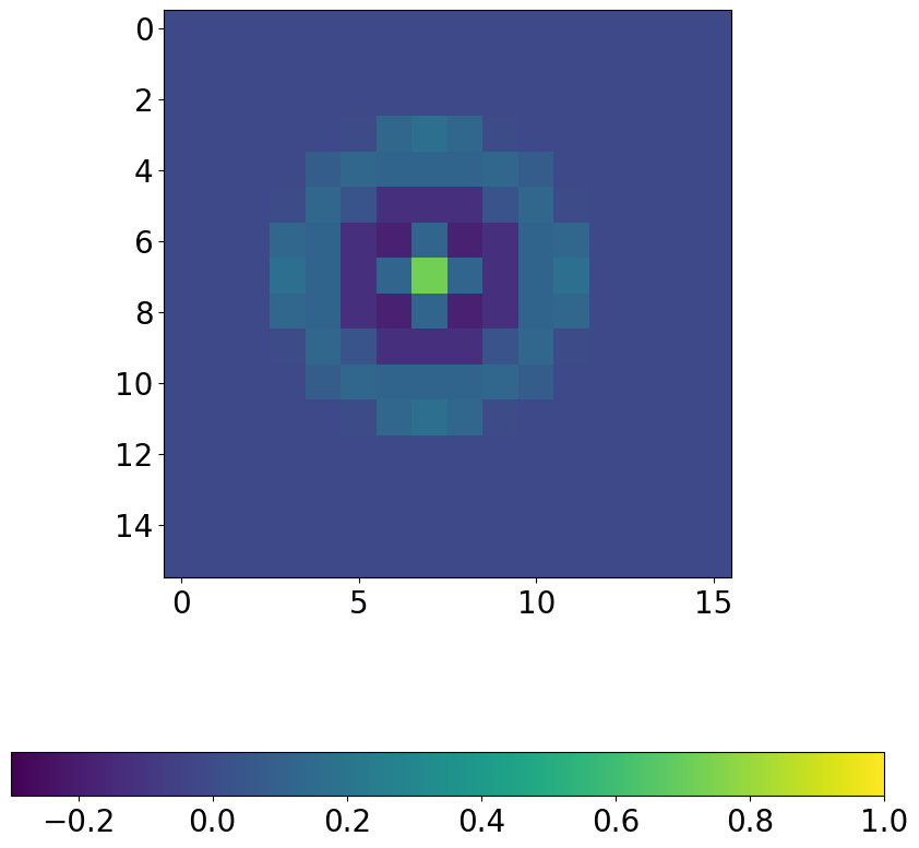
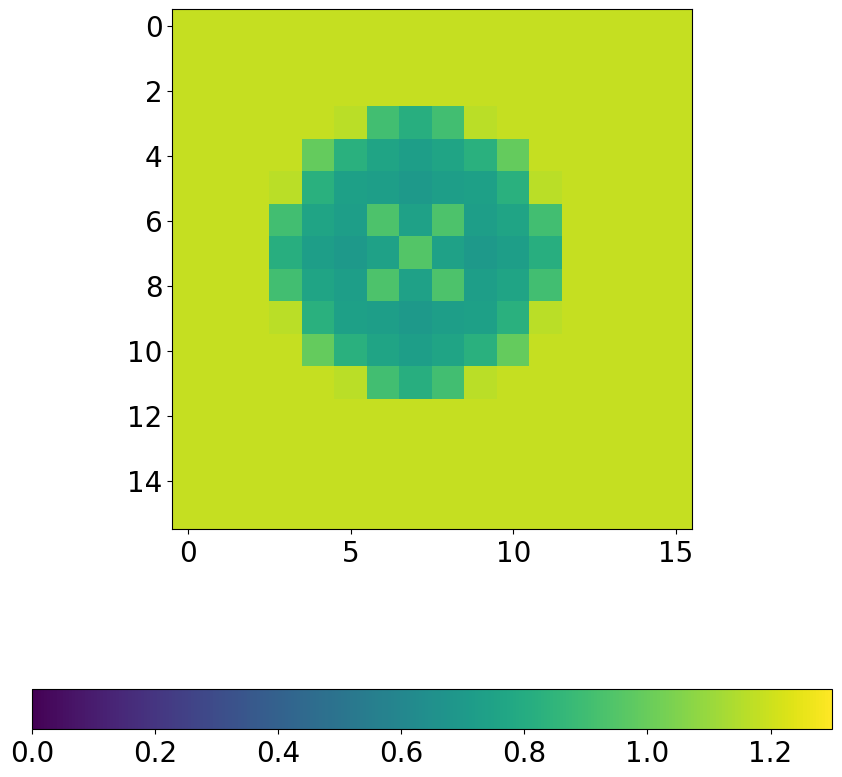
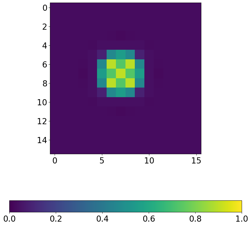
The initial and learnt values for $y^{\prime}_{\theta},v^{\scriptscriptstyle+}_{\theta},m_{\theta}$ of our Global-GOCor module are visualized in Figure 6. They result from the training of GLU-Net-GOCor on the synthetic Dynamic training dataset. We additionally provide the visualization of $y_{ij..},v^{\scriptscriptstyle-}_{ij..},v^{\scriptscriptstyle+}_{ij..}\in\mathbb{R}^{H\times W}$ as heat-maps for a particular location $(i,j)$ in Figure 7.

Figure 6: Plot of the learnt target confidence $y^{\prime}_{\theta}$ and weights $v^{\scriptscriptstyle+}_{\theta},m_{\theta}$. The learnt values are shown in red while the initialization of each function is presented in green.

(a) Initial Label $y_{ij..}$

(b) Initial Weight $v^{\scriptscriptstyle+}_{ij..}$

(c) Initial Weight $v^{\scriptscriptstyle-}_{ij..}$

(d) Learnt Label $y_{ij..}$

(e) Learnt Weight $v^{\scriptscriptstyle+}_{ij..}$

(f) Learnt Weight $v^{\scriptscriptstyle-}_{ij..}$

Figure 7: Visualization of the heat maps corresponding to the learnt target confidence $y$ and weights $v^{\scriptscriptstyle-},v^{\scriptscriptstyle+}$ for a particular location $(i,j)=(7,7)$. (a), (b) and (c) show the initialization of each function while (d), (e) and (f) depict the learnt values.

Smoothness operator $\mathbf{R_{\theta}}$: We now focus on the operator $R_{\theta}$, introduced in the loss formulation on the query image in Sec. 3.5. $R_{\theta}\in\mathbb{R}^{K^{4}\times Q}$ is a learnable 4D-kernel of spatial size $K$ and $Q$ number of output channels. We set $K=3$ and $Q=16$ output channels. For implementation purposes, the 4-D convolution is factorized as two consecutive 2-D convolutional layers, operating over the two first and two latter dimensions respectively. The output dimension of the first 2D-convolution is also set to 16. Note that the kernel $R_{\theta}$ is learnt, along with all other network parameters, by the SGD-based minimization of the same final network training loss used in the GLU-Net and PWC-Net baselines. This is contrary to the filter map $w$ that is optimized using Eq. 5 and 6 at each forward pass of the network.

Appendix D Experimental setup and datasets

In this section, we first provide details about the evaluation metrics and datasets. We then explain the procedure used to create the Dynamic dataset, utilized for training state-of-the-art GLU-Net. Finally, we detail the architecture of our baseline network, used for our ablation study, namely BaseNet.

D.1 Evaluation metrics

AEPE: AEPE is defined as the Euclidean distance between estimated and ground truth flow fields, averaged over all valid pixels of the reference image.

PCK: The Percentage of Correct Keypoints (PCK) is computed as the percentage per image, of correspondences $\mathbf{\tilde{x}}_{j}$ with an Euclidean distance error $\left\|\mathbf{\tilde{x}}_{j}-\mathbf{x}_{j}\right\|\leq T$, w.r.t. to the ground truth $\mathbf{x}_{j}$, that is smaller than a threshold $T$. Note that all PCK percentages presented, except for the ones reported on MegaDepth, are computed per image and then averaged over all image pairs of the dataset. On MegaDepth however, following [52], the PCK are calculated over all valid pixels of the dataset.

F1: F1 designates the percentage of outliers averaged over all valid pixels of the dataset [17]. They are defined as follows, where $F_{gt}$ indicates the ground-truth flow field and $F$ the estimated flow by the network.

$$F1=\frac{\left\|F-F_{gt}\right\|>3\textrm{ and }\frac{\left\|F-F_{gt}\right\|}{\left\|F_{gt}\right\|}>0.05}{\textrm{\#valid pixels}}$$ (30)

D.2 Evaluation datasets

HP: The HPatches dataset [3] is a benchmark for geometric matching correspondence estimation. It depicts planar scenes, with transformations restricted to homographies. We only employ the 59 sequences labelled with v_X, which have viewpoint changes, thus excluding the ones labelled i_X, which only have illumination changes. Each image sequence contains a query image and 5 reference images taken under increasingly larger viewpoints changes, with sizes ranging from $450\times 600$ to $1613\times 1210$.

ETH3D: To validate our approach for real 3D scenes, where image transformations are not constrained to simple homographies, we also employ the Multi-view dataset ETH3D [51]. It contains 10 image sequences at $480\times 752$ or $514\times 955$ resolution, depicting indoor and outdoor scenes and resulting from the movement of a camera completely unconstrained, used for benchmarking 3D reconstruction. The authors additionally provide a set of sparse geometrically consistent image correspondences (generated by [49]) that have been optimized over the entire image sequence using the reprojection error. We sample image pairs from each sequence at different intervals to analyze varying magnitude of geometric transformations, and use the provided points as sparse ground truth correspondences. This results in about 500 image pairs in total for each selected interval. Note that the PCK and AEPE values computed per image are then averaged over all image pairs of each sequence. The final metrics presented are the averages over all sequences.

MegaDepth: To validate our approach on real scenes depicting extreme viewpoint changes, we use images of the MegaDepth dataset. No real ground-truth correspondences are available, so we use the result of SfM reconstructions to obtain sparse ground-truth correspondences. We follow the same procedure and test images than [52]. More precisely, we use 3D points and project them onto pairs of matching images to obtain correspondences and we randomly sample 1600 pairs of images that shared more than 30 points. It results in approximately 367K correspondences. Note that for evaluation, following [52], the PCK metrics are calculated over all valid pixels of the dataset.

KITTI: The KITTI dataset [17] is composed of real road sequences captured by a car-mounted stereo camera rig. The KITTI benchmark is targeted for autonomous driving applications and its semi-dense ground truth is collected using LIDAR. The 2012 set only consists of static scenes while the 2015 set is extended to dynamic scenes via human annotations. The later contains large motion, severe illumination changes, and occlusions.

Sintel: The Sintel benchmark [8] is created using the open source graphics movie “Sintel” with two passes, clean and final. The final pass contains strong atmospheric effects, motion blur, and camera noise.

TSS: The TSS dataset [58] contains 400 image pairs, divided into three groups: FG3DCAR, JODS, and PASCAL, according to the origins of the images. The dense flow fields annotations for the foreground object in each pair is provided along with a segmentation mask. Evaluation is done on 800 pairs, by also exchanging query and reference images.

D.3 Training dataset for GLU-Net based networks

In [59], GLUNet is trained on DPED-ADE-CityScapes, created by applying synthetic affine, TPS and homography transformations to real images of the DPED [23], CityScapes [14] and ADE-20K [66] datasets. Here, we refer to this dataset as the Static training dataset, since it simulates a static scene. While GLU-Net trained on the Static dataset obtains state-of-the-art results on geometric matching and optical flow datasets (see Table 7), the Static dataset does not capture independently moving objects, present in optical flow data. For this reason, we introduce a Dynamic training dataset, created from the original Static dataset with additional random independently moving objects. To do so, these objects are sampled from the COCO dataset [36], and inserted on top of the images of the Static data using their segmentation masks. To generate motion, we randomly sample affine transformation parameters for the foreground objects, which are independent of the background transformations. This can be interpreted as both the camera and the objects moving independently of each other. The Dynamic dataset allows the network to learn the presence of independently moving objects and motion boundaries.

In Table 7, we compare evaluation results of original GLU-Net trained on either the Static or the Dynamic datasets. While training on the Dynamic data leads to worse results on HPatches, it leads to improved performances on all optical flow data, particularly significant on Sintel and KITTI-2015. Only the F1 metric on KITTI-2012 is slightly worse when training on the Dynamic dataset. This is consistent with the fact that the Static training dataset is in line with HPatches, both restricted to homography transformations, while the Dynamic one is better suited for optical flow data, that depict independently moving objects. The Dynamic dataset is especially suitable for KITTI-2015 and Sintel, since both represent dynamic scenes, while KITTI-2012 only experiences static 3D scenes.

Results on HPatches and TSS are computed with GLU-Net and GLU-Net-GOCor trained on the Static dataset while results on MegaDepth, ETH3D and optical flow data KITTI and Sintel use the networks trained on the Dynamic data instead. Here, we emphasize that both GLU-Net and GLU-Net-GOCor are trained with exactly the same procedure, introduced in [59].

Table 7: Evaluation results of GLU-Net when trained on the Static or the Dynamic datasets.

	HP		KITTI-2012		KITTI-2015		Sintel-Cleam		Sintel-Final
	AEPE $\downarrow$	PCK-5 [%] $\uparrow$	AEPE $\downarrow$	F1 [%] $\downarrow$	AEPE $\downarrow$	F1 [%] $\downarrow$	AEPE $\downarrow$	PCK-5 [%] $\uparrow$	AEPE $\downarrow$	PCK-5 [%] $\uparrow$
GLU-Net (Static)	25.05	78.54	3.34	18.93	9.79	37.52	6.03	84.21	7.01	81.92
GLU-Net (Dynamic)	27.01	78.37	3.14	19.76	7.49	33.83	4.25	88.40	5.50	85.10

(a) BaseNet

(b) BaseNet-GOCor

Figure 8: Schematic representation of BaseNet and BaseNet-GOCor, estimating dense flow field w from a pair of reference and query images.

D.4 Architecture and training of BaseNet

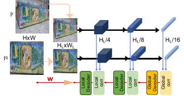
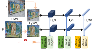
We introduce BaseNet, a simpler version of GLU-Net [59], estimating the dense flow fields relating a pair of images. The network is composed of three pyramid levels and it uses VGG-16 [9] as feature extractor backbone. The coarsest level is based on a global correlation layer, followed by a mapping decoder estimating the correspondence map at this resolution. The two next pyramid levels instead rely on local correlation layers. The dense flow field is then estimated with flow decoders, taking as input the correspondence volumes resulting from the local feature correlation layers. Besides, BaseNet is restricted to a pre-determined input resolution $H_{L}\times W_{L}=256\times 256$ due to its global correlation at the coarsest pyramid level. It estimates a final flow-field at a quarter of the input resolution $H_{L}\times W_{L}$, which needs to be upsampled to original image resolution $H\times W$. The mapping and flow decoders have the same architecture as those used for GLU-Net [59].

To create BaseNet-GOCor, we simply replace the global and local correlation layers by respectively our global and local GOCor modules. In the standard BaseNet, the correspondence volume generated by the global correlation layer is passed through a ReLU non linearity [40] and further L2-normalized in the channel dimension, to enhance high correlation values and to down-weight noise values. While beneficial for the standard feature correlation layer, we found the L2-normalization to be slightly harmful for the performance when using our GOCor module. Indeed, our GOCor module inherently already suppresses correlation values at ambiguous matches while enhancing the correct match. We therefore only pass the correspondence volume through a Leaky-ReLU. The rest of the architecture remains unchanged. Schematic representations of BaseNet and BaseNet-GOCor are presented in Figure 8.

Both networks are trained end-to-end, following the same procedure introduced in [59]. We set the batch size to 40 and the initial learning rate of $10^{-3}$, which is further reduced during training.

Appendix E Additional results

Here, we first look at the impact of the number of Steepest Descent iterations used within the filter predictor module during inference in section E.1. In section E.2, we then give more detailed results for the task of geometric matching. We subsequently provide an extended table of results on optical flow datasets in section E.3 as well as additional results on the ETH3D dataset. We then illustrate the superiority of our approach through multiple qualitative examples in section E.5. Finally, we compare results for different loss parametrization in section E.6.

Note that for GLU-Net and GLU-Net-GOCor, results on HPatches and TSS are computed with the networks trained on the Static dataset while results on MegaDepth, ETH3D and optical flow data KITTI and Sintel use the networks trained on the Dynamic data instead. All presented results of GLU-Net-GOCor and PWC-Net-GOCor use 3 global optimization iterations (when applicable) and 7 local optimization iterations. Only on the TSS dataset, we compute metrics for GLU-Net-GOCor with only 3 local optimization iterations. This is because on semantic data, depicting different instances of the same object, the value of the reference objective is less pronounced compared to geometric and optical flow data, for which image pairs represent the same scene. Therefore, on semantic data, using too many local optimization iterations can be harmful.

(a) HPatches

(b) KITTI-2012

(b) Sintel-clean

Figure 9: Evaluation results of GLU-Net-GOCor and PWC-Net-GOCor when increasing the number of steepest descent iterations in either the global or the local GOCor modules. While increasing the number of global iterations, the number of local iterations is fixed to three, and similarly. Note that GLU-Net-GOCor was trained on the Dynamic dataset and PWC-Net-GOCor was trained on 3D-Things. Both networks were trained with three steepest descent iterations for both the local and global GOCor modules, if applicable.

E.1 Impact of number of inference Steepest Descent iterations

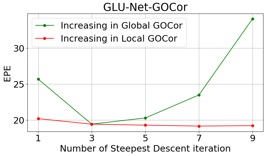
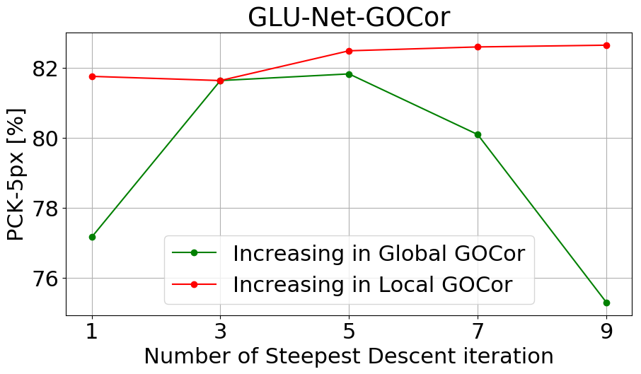
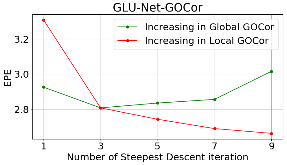
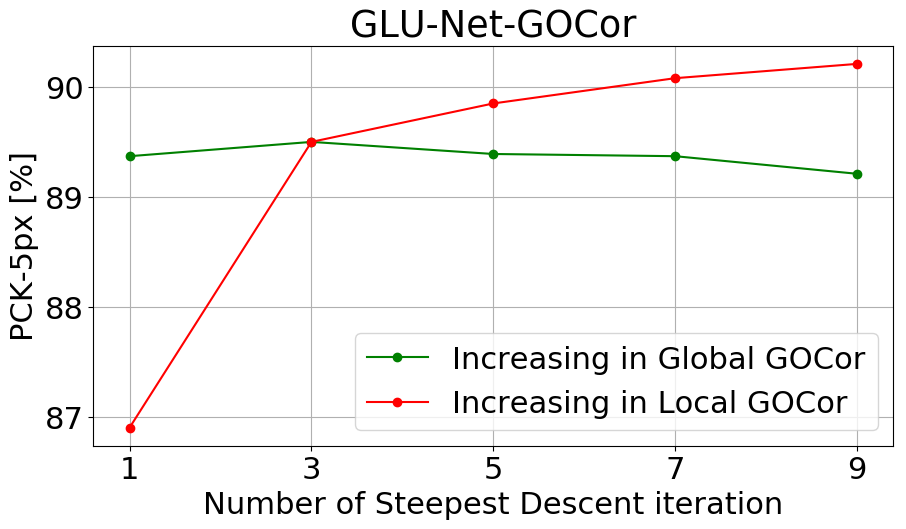
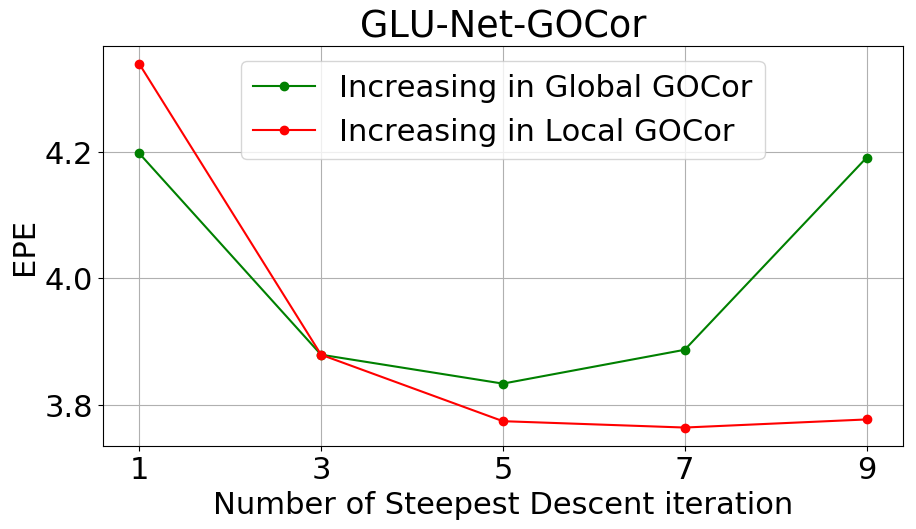
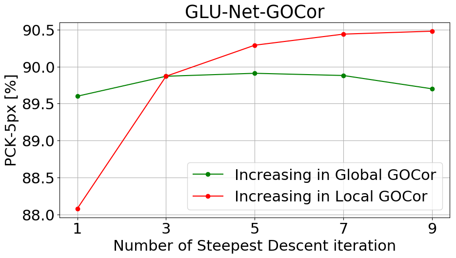
Impact on performance: Here, we analyse the impact of the number of Steepest Descent iterations in the global and local GOCor modules used during inference, on the performance of the corresponding network. We first focus on the global GOCor module. In Figure 9, we plot the AEPE and PCK-5px obtained by GLU-Net-GOCor when increasing the number of global steepest descent iterations during inference. Note that the network was trained with three global iterations. On both HPatches and KITTI-2012, GLU-Net-GOCor with three global iterations, i.e. with the same number of iterations than used during training, leads to the best performance. Increasing or decreasing the number of global iterations leads to a significant drop in performance. This is primarily due to our query frame objective (Sec. 3.5 of the main paper), which learns the optimal regularizer weights for the number of steepest descent iterations used during training.

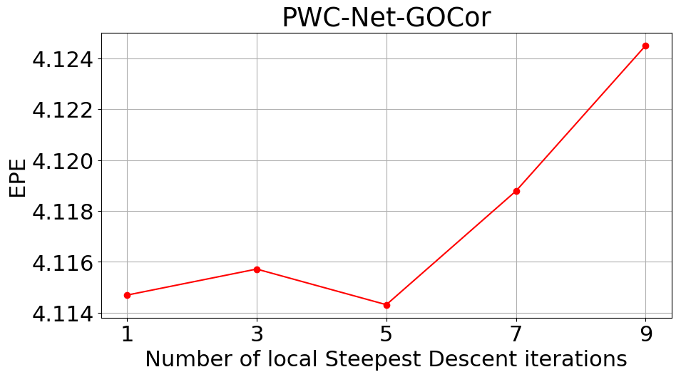
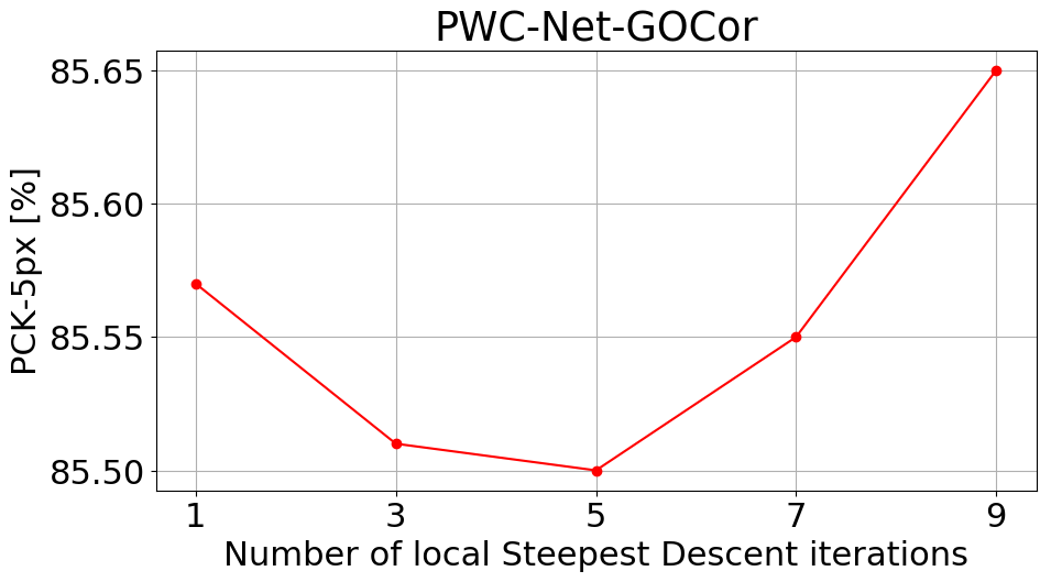
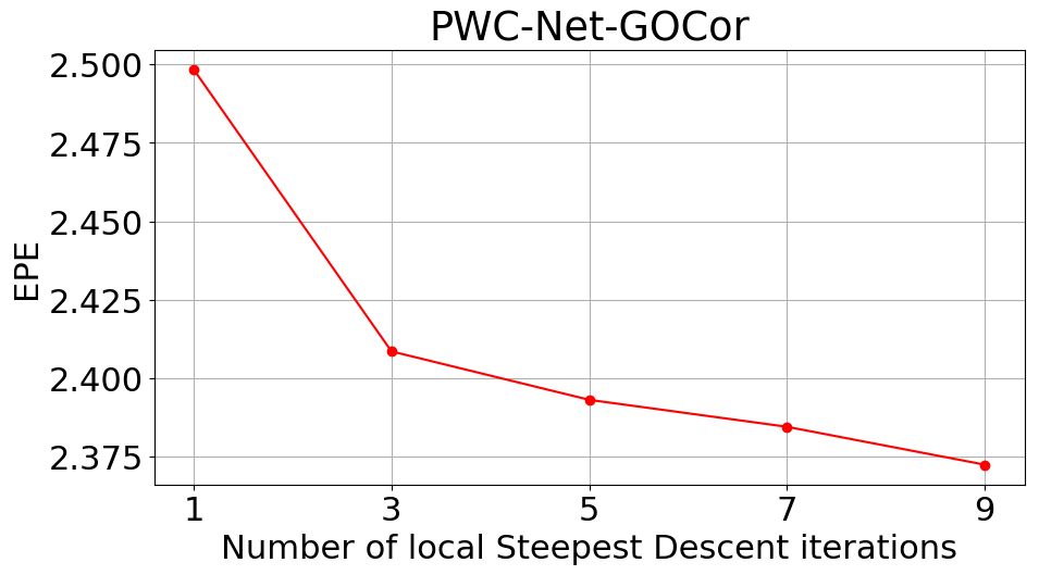
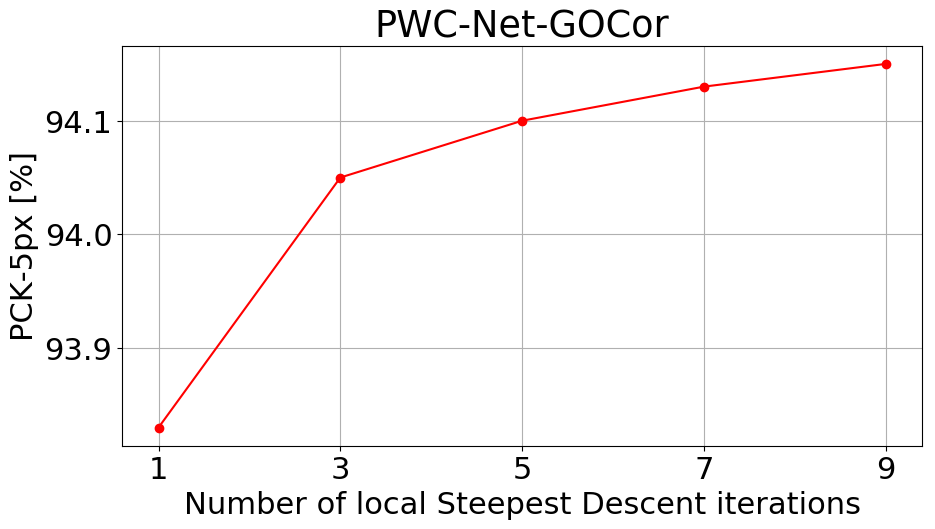
We next look at the impact of the number of steepest descent iterations used in the local GOCor module. In Figure 9, we thus plot the AEPE and PCK-5px of GLU-Net-GOCor and PWC-Net-GOCor for different inference number of local optimization iterations. Both networks were trained with three such iterations. Increasing the number of local steepest descent iterations during inference improves the network performances on all datasets. On KITTI-2012 only, the trend is slightly different, however the difference in performance for different number of iterations is insignificant, in the order of 0.01. It is important to note that in the local GOCor module, we only use our robust loss in the reference frame (Sec. 3.4), ignoring the loss on the query frame (Sec. 3.5). Therefore, increasing the number of iterations during inference will in that case make the predicted filter map $w_{ij}$ at location $(i,j)$ more and more discriminative to reference feature $f^{r}_{ij}$. The final correspondence volume obtained from applying optimized $w^{*}$ to the query feature map will thus be more accurate.

Taking into consideration solely the performance gain, in the global-GOCor, the best alternative during inference is to use the same number of steepest descent iterations than during training (i.e. three iterations here). For the local-GOCor on the other hand, increasing the number of inference steepest descent iterations leads to better resulting network metrics. However, one must take into account that while increasing the number of inference iterations in the local GOCor module leads to improved performances, it also results in increased inference run-time.

Table 8: Run time of our method compared to original versions of PWC-Net and GLU-Net, averaged over the 194 image pairs of KITTI-2012. The number of optimization iterations is indicated for the local-GOCor modules. For GLU-Net-GOCor, we use three steepest descent iterations in the global-GOCor.

	PWC-Net	PWC-Net-GOCor	PWC-Net-GOCor	GLU-Net	GLU-Net-GOCor	GLU-Net-GOCor
		optim-iter = 3	optim-iter = 7		optim-iter = 3	optim-iter = 7
Run-time [ms]	118.05	166.00	203.02	154.97	211.02	261.90

Impact on run-time: We thus compare the run-time of our GOCor-networks for different number of optimization iterations in the local GOCor module. For reference, we additionally compare them to their corresponding original networks GLU-Net and PWC-Net. The run-times computed on all images of the KITTI-2012 images are presented in Table 8. The timings have been obtained on the same desktop with an NVIDIA Titan X GPU. All networks output a flow at a quarter resolution of the input images. We up-scale to the image resolution with bilinear interpolation. This up-scaling operation is included in the estimated time.

Therefore, we found that setting seven steepest descent iterations during inference in the local GOCor was a good compromise between excellent performance and reasonable run-time. All results in the main paper are indicated with this setting. Nevertheless, for time-demanding applications, only using three local optimization iterations (i.e. the same number than during training) results in faster GOCor-networks with still a significant performance gain compared to their original feature correlation layer-based networks.

Figure 10: Visualization of the flow field estimated by GLU-Net and GLU-Net-GOCor for different steepest descent iterations during inference. The image pair is extracted from the clean pass of Sintel. The first number indicates the number of optimization iterations in the global GOCor module while the second refer to the number of steepest descent iterations in the local GOCor module. Both GLU-Net and GLU-Net-GOCor were trained on the Dynamic dataset. GLU-Net-GOCor was trained with three steepest descent iterations for both the local and global GOCor modules.

In Figure 10, we visualize the estimated flow field for a pair of Sintel images, by GLU-Net and GLU-Net-GOCor for different optimization iterations. It is very clear that increasing the number of optimization iterations leads to a more accurate estimated flow field. In particular, the estimated flow field becomes more detailed, with well-defined motion boundaries.

E.2 Additional geometric matching results

Detailed results obtained by GLU-Net and GLU-Net-GOCor on the various view-points of the HP dataset are presented in Table 9. It extends Table 1 of the main paper, that only provides the average over all viewpoint IDs. In addition to the Average End-Point Error (AEPE), we also provide the standard deviation over the End-Point Error per image. It represents the distribution of EPE per image, averaged over all images of each view-point. Note that increasing view-point IDs lead to increasing geometric transformations due to larger changes in viewpoint.

Our approach GLU-Net-GOCor outperforms original GLU-Net for each viewpoint ID. Particularly, GLU-Net-GOCor is significantly more robust for large view-point changes, such as those experienced in Viewpoint V, with an AEPE of 38.41 against 51.47 for original GLU-Net. Besides, GLU-Net-GOCor always obtains a narrower distribution of errors. This implies that our approach enables the network to have a more steady performance over the whole dataset.

Table 9: Details of AEPE and PCK evaluated over each view-point ID of the HPatches dataset. All methods are trained on the Static dataset.

		I	II	III	IV	V	all
	AEPE $\downarrow$	1.55 $\pm$ 1.80	12.66 $\pm$ 10.43	27.54 $\pm$ 16.05	32.04 $\pm$ 20.01	51.47 $\pm$ 94.77	25.05 $\pm$ 16.67
GLU-Net	PCK-1px [%] $\uparrow$	61.72	42.43	40.57	29.47	23.55	39.55
	PCK-5px [%] $\uparrow$	96.15	84.35	79.46	73.80	58.92	78.54
	AEPE $\downarrow$	1.29 $\pm$ 1.31	10.07 $\pm$ 7.44	23.86 $\pm$ 14.01	27.17 $\pm$ 16.84	38.41 $\pm$ 28.52	20.16 $\pm$ 13.63
GLU-Net-GOCor	PCK-1px [%] $\uparrow$	64.93	43.86	42.52	30.68	25.78	41.55
	PCK-5px [%] $\uparrow$	96.95	86.41	82.47	76.17	65.15	81.43

E.3 Additional optical flow results

Extended optical flow results: Table 10 here extends Table 3 in the paper with more results on optical flow datasets. Specifically, we compare our approaches with other state-of-the-art networks applied to the train splits of the KITTI and Sintel datasets. Similarly to PWC-Net, these other methods, such as LiteFlowNet [21], rely on local correlation layers at multiple levels to infer the final flow field relating a pair of images. Our local GOCor module could therefore easily be integrated into any of these networks in place of the local correlation layers.

In Table 10, PWC-Net* refers to the results presented in the original PWC-Net publication [55]. In the middle section, we show the evaluation results of PWC-Net*, as well as PWC-Net-GOCor and PWC-Net both further finetuned on 3D-Things according to the same schedule. In the last section of the table, we focus on the PWC-Net variants finetuned on the Sintel training dataset. For a fair comparison, we here also provide the official PWC-Net* ft Sintel results, as well as the PWC-Net-GOCor and PWC-Net versions that we finetuned on Sintel. Our PWC-Net-GOCor outperforms both PWC-Net* and PWC-Net on the KITTI data by a large margin, while obtaining similar results on the training set of Sintel. As already mentioned in Section 4.2 of the main paper, this highlights the generalization capabilities of our GOCor module.

Table 10: Results for the optical flow task on the training splits of KITTI [17] and Sintel [8]. A result in parenthesis indicates that the dataset was used for training. PWC-Net* indicates the results stated in the original PWC-Net paper [55]. For all methods, the training dataset is indicated in parenthesis next to the method. When not indicated, the method was trained on Flying-Chairs [16] followed by 3D-Things [24].

	KITTI-2012		KITTI-2015		Sintel Clean			Sintel Final
	AEPE $\downarrow$	F1 (%) $\downarrow$	AEPE $\downarrow$	F1 (%) $\downarrow$	AEPE $\downarrow$	PCK-1 (%) $\uparrow$	PCK-5 (%) $\uparrow$	AEPE $\downarrow$	PCK-1 (%) $\uparrow$	PCK-5 (%) $\uparrow$
GLU-Net (Dynamic)	3.14	19.76	7.49	33.83	4.25	62.08	88.40	5.50	57.85	85.10
GLU-Net-GOCor (Dynamic) (Ours)	2.68	15.43	6.68	27.57	3.80	67.12	90.41	4.90	63.38	87.69
FlowNet2.0 [24]	4.09	-	10.06	30.37	2.02	-	-	3.14	-	-
SpyNet [44]	9.12	-	-	-	4.12	-	-	6.69	-	-
LiteFlowNet [21]	4.00	-	10.39	28.50	2.48	-	-	4.04	-	-
LiteFlowNet2 [22]	3.42	-	8.97	25.88	2.24	-	-	3.78	-	-
PWC-Net*	4.14	21.38	10.35	33.67	2.55	-	-	3.93	-	-
PWC-Net (ft 3D-Things)	4.34	20.90	10.81	32.75	2.43	81.28	93.74	3.77	76.53	90.87
PWC-Net-GOCor (ft 3D-Things) (Ours)	4.12	19.31	10.33	30.53	2.38	82.17	94.13	3.70	77.34	91.20
FlowNet2 (ft Sintel)	3.54	-	9.94	28.02	(1.45)	-	-	(2.19)	-	-
PWC-Net* (ft Sintel)	2.94	12.70	8.15	24.35	(1.70)	-	-	(2.21)	-	-
PWC-Net (ft Sintel)	2.87	11.97	8.68	23.82	(1.76)	(87.24)	(95.37)	(2.23)	(83.61)	(93.61)
PWC-Net-GOCor (ft Sintel) (Ours)	2.60	9.67	7.64	20.93	(1.74)	(87.93)	(95.54)	(2.28)	(84.15)	(93.71)

Here, we also present the evaluation results on the test set of the Sintel dataset in Table 11. We compare PWC-Net and PWC-Net-GOCor, both finetuned on the training split of Sintel. For reference and as previously, we also present the official results from the PWC-Net publication [55], denoted as PWC-Net*. PWC-Net-GOCor outperforms both PWC-Net and PWC-Net* on the clean pass. On the final pass, PWC-Net-GOCor obtains better performance than PWC-Net, but slightly worse results than PWC-Net*. The authors of PWC-Net employ special data augmentation strategies and training procedures for fine-tuning, which are not shared as PyTorch code by the authors. The finetuning procedure that we employed for our PWC-Net-GOCor and standard PWC-Net is therefore different from the one used for in the official PWC-Net results (PWC-Net*). However, we finetuned both PWC-Net and PWC-Net-GOCor with the same setting and procedure, enabling fair comparison between the two. PWC-Net-GOCor performs particularly better in regions with large motions and close to the motion boundaries. This is in line with the behavior of the GOCor module observed previously, according to which the GOCor module particularly improves performance on large displacements.

Table 11: Detailed results on the test set of Sintel benchmark for different regions, velocities (s), and distances from motion boundaries (d). All methods are trained on Flying-Chairs [16] followed by 3D-Things [24], and further finetuned on the training split of Sintel.

	Sintel-Clean
	EPE-all	EPE matched	EPE unmatched	d0-10	d10-60	d60-140	s0-10	s10-40	s40+
PWC-Net* (ft-Sintel)	4.386	1.719	26.166	4.282	1.657	0.657	0.606	0.2070	28.783
PWC-Net (ft-Sintel)	4.637	1.951	26.571	4.018	1.626	1.040	0.649	2.070	30.671
PWC-Net-GOCor (ft-Sintel)	4.195	1.660	24.909	3.843	1.448	0.778	0.609	1.914	27.552
	Sintel-Final
	EPE-all	EPE matched	EPE unmatched	d0-10	d10-60	d60-140	s0-10	s10-40	s40+
PWC-Net* (ft-Sintel)	5.042	2.445	26.221	4.636	2.087	1.475	0.799	2.986	31.070
PWC-Net (ft-Sintel)	5.300	2.576	27.528	4.717	2.204	1.580	0.929	2.994	32.584
PWC-Net-GOCor (ft-Sintel)	5.133	2.458	26.945	4.504	2.063	1.603	0.834	2.906	31.858

Table 12: AEPE/F1 [%] on KITTI-2015.

	Not occluded	Occluded	All
GLU-Net	4.67 / 27.83	21.95 / 67.44	7.49 / 33.83
GLU-Net-GOCor	4.22 / 22.03	19.07 / 58.61	6.68 / 27.57
PWC-Net	5.40 / 25.16	34.39 / 78.58	10.81 / 32.75
PWC-Net-GOCor	5.02 / 23.53	34.06 / 77.84	10.33 / 30.53

Performance on occlusion data: Here, we focus specifically on the performance of GOCor in occluded regions. As shown in Tab. 11, in occluded regions (“EPE unmatched”) of the Sintel test set, GOCor provides relative improvements of 6.25% and 2.16% on the clean and final pass respectively. In Tab. 12, we present the details of the metrics on occluded and non-occluded regions of KITTI-2015. GOCor improves the performance of PWC-Net and GLU-Net in occluded regions of a substantial amount as compared to the feature correlation layer.

Figure 11: Quantitative results on ETH3D [51] images. AEPE, PCK-1 and PCK-5 are computed on pairs of images sampled from consecutive images of ETH3D at different intervals. PWC-Net* refers to the official pre-trained weights provided by the authors.

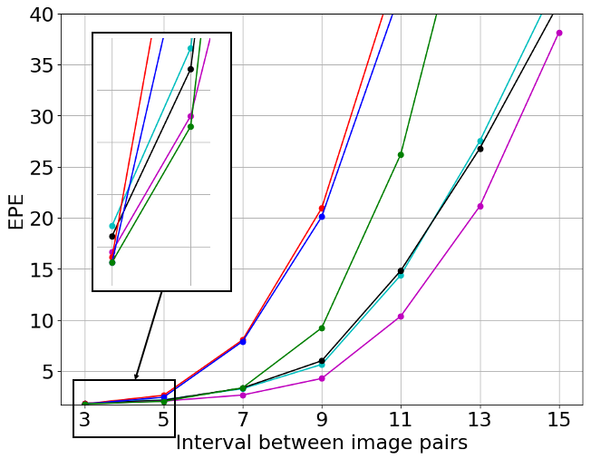
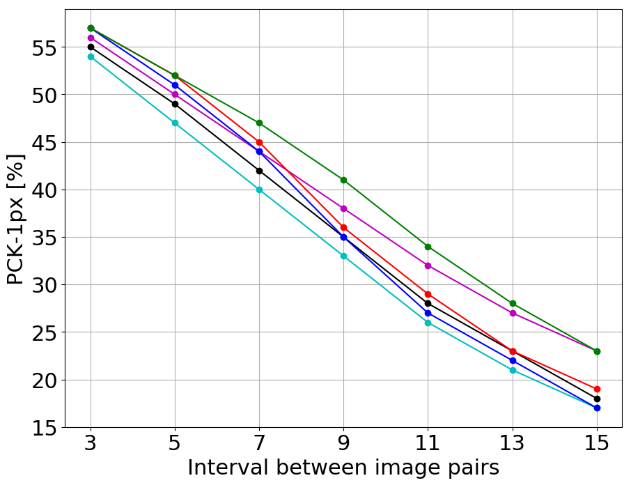
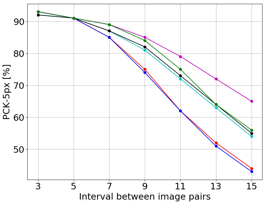
E.4 Additional results on ETH3D

In the main paper, Figure 4, we quantitatively evaluated our approach over pairs of ETH3D images sampled from consecutive frames at different intervals. For completeness, in Figure 11, we also present the evaluation results of PWC-Net and PWC-Net-GOCor applied to the ETH3D images, sampled at increasingly high intervals. Indeed, for small intervals, finding correspondences strongly resembles optical flow task while increasing the interval leads to larger displacements. Optical flow network PWC-Net can thus be very suitable, particularly when estimating the flow at small intervals. In Figure 11, both PWC-Net and PWC-Net-GOCor are finetuned on 3D-Things according to the same schedule. For reference, we additionally provide the results of PWC-Net*, which refers to the official pre-trained weights provided by the authors, after training on Flying-chairs and 3D-Things. We also provide the results of PWC-Net*, PWC-Net and PWC-Net-GOCor further finetuned on Sintel.

For all intervals, and independently of the dataset it was trained on, our approach PWC-Net-GOCor obtains better metrics than both PWC-Net and PWC-Net*. Particularly, the gap in performance broadens with the intervals between the frames, implying that our module is especially better at handling large view-point changes. This is especially obvious for the networks finetuned on Sintel. Indeed, as further evidenced in Tab. 13, PWC-Net and PWC-Net* finetuned on Sintel experience a very large drop in performance on all metrics from a frame interval of 7, as compared to PWC-Net-GOCor finetuned on the same data. This particular robustness to large displacements was similarly observed when our GOCor modules were integrated into GLU-Net (Sec. 4.1). It highlights that the improved performances brought by our GOCor approach compared to the feature correlation layer generalize to different networks.

In Table 13, we give the corresponding detailed evaluation metrics (AEPE and PCK) obtained by geometric matching networks DGC-Net, GLU-Net, GLU-Net-GOCor and optical flow models LiteFlowNet, PWC-Net, PWC-Net* and PWC-Net-GOCor.

Table 13: Metrics evaluated over scenes of ETH3D with different intervals between consecutive pairs of images (taken by the same camera). Note that those results are the average over the different sequences of the ETH3D dataset. Small AEPE and high PCK are better.

(a) Geometric matching methods
DGC-Net GLU-Net GLU-Net GLU-Net-GOCor [39] Static = DPED-CityScape-ADE in [59] Dynamic Dynamic AEPE 2.49 1.98 2.01 1.93 interval = 3 PCK-1px [%] 34.19 50.55 46.27 47.97 PCK-5px [%] 88.50 91.22 91.45 92.08 AEPE 3.28 2.54 2.46 2.28 interval = 5 PCK-1px [%] 27.22 43.08 39.28 41.79 PCK-5px [%] 83.25 87.91 88.57 89.87 AEPE 4.18 3.48 2.98 2.64 interval = 7 PCK-1px [%] 22.45 36.98 34.05 36.81 PCK-5px [%] 78.32 84.23 85.64 87.77 AEPE 5.35 4.23 3.51 3.01 interval = 9 PCK-1px [%] 18.82 32.45 30.11 33.03 PCK-5px [%] 73.74 80.74 83.10 85.88 AEPE 6.78 5.59 4.30 3.62 interval = 11 PCK-1px [%] 15.82 28.45 26.69 29.80 PCK-5px [%] 69.23 76.84 80.12 83.69 AEPE 9.02 7.54 6.11 4.79 interval = 13 PCK-1px [%] 13.49 25.06 23.73 26.93 PCK-5px [%] 64.28 72.35 76.66 81.12 AEPE 12.25 10.75 9.08 7.80 interval = 15 PCK-1px [%] 11.25 21.89 20.85 23.99 PCK-5px [%] 58.66 67.77 73.02 77.90
(b) Optical flow methods
LiteFlowNet PWC-Net* PWC-Net PWC-Net-GOCor PWC-Net PWC-Net-GOCor Chairs-Things Chairs-Things Chairs-Things Chairs-Things ft Sintel ft Sintel AEPE 1.67 1.75 1.73 1.70 1.68 1.67 interval = 3 PCK-1px [%] 61.63 57.54 58.50 58.93 59.93 60.46 PCK-5px [%] 92.79 92.62 92.64 92.81 92.89 92.92 AEPE 2.58 2.10 2.06 1.98 2.35 1.95 interval = 5 PCK-1px [%] 56.55 50.41 52.02 53.10 54.41 55.54 PCK-5px [%] 90.70 90.71 90.82 91.45 91.10 91.59 AEPE 6.05 3.21 3.28 2.58 7.83 3.29 interval = 7 PCK-1px [%] 49.83 42.95 44.86 46.91 46.76 50.37 PCK-5px [%] 86.29 87.04 87.32 88.96 85.21 89.51 AEPE 12.95 5.59 5.95 4.22 20.05 9.16 interval = 9 PCK-1px [%] 42.00 35.23 37.41 40.93 37.24 44.33 PCK-5px [%] 78.50 81.17 81.80 85.53 73.90 84.65 AEPE 29.67 14.35 14.79 10.32 42.17 26.16 interval = 11 PCK-1px [%] 33.14 28.14 30.36 34.58 29.24 36.91 PCK-5px [%] 66.07 71.91 72.95 79.44 61.64 75.49 AEPE 52.41 27.49 26.76 21.10 67.79 56.47 interval = 13 PCK-1px [%] 26.46 22.91 24.75 29.25 23.40 30.27 PCK-5px [%] 55.05 63.19 64.07 72.06 51.31 63.79 AEPE 74.96 43.41 40.99 38.12 94.59 83.18 interval = 15 PCK-1px [%] 21.22 18.34 19.89 24.59 18.72 25.17 PCK-5px [%] 46.29 54.39 55.47 64.92 43.22 55.84

E.5 Qualitative examples

Here, we first present qualitative comparisons of PWC-Net and PWC-Net-GOCor. In Figure 13, we show examples of PWC-Net and PWC-Net-GOCor applied to images of optical flow datasets KITTI-2012 and KITTI-2015. Both networks are trained on 3D-Things. PWC-Net-GOCor shows more defined motion boundaries and generally more accurate estimated flow fields. Similarly, we present examples on the clean pass of the Sintel training set in Figure 14. PWC-Net-GOCor captures more detailed flow fields. This is for instance illustrated in the first example of Figure 14, where PWC-Net-GOCor correctly identified the foot contrary to PWC-Net, which failed to capture it. However, both PWC-Net and PWC-Net-GOCor may fail on small and rapidly moving objects, such as the arm in the last example of Figure 14.

In Figure 15, we additionally present qualitative results on the KITTI images when the networks are finetuned on Sintel. Indeed, in Table 10, we showed that while both PWC-Net and PWC-Net-GOCor obtain very similar results on training data Sintel, PWC-Net-GOCor performs largely better on the KITTI datasets compared to original PWC-Net, especially in terms of F1 metric. PWC-Net-GOCor also obtains visually more accurate flow fields on the KITTI images.

Besides, we show the advantage of our approach as compared to the feature correlation layer when integrated in GLU-Net. In Figure 16, we visually compare GLU-Net and GLU-Net-GOCor when applied to images of the clean pass of the Sintel benchmark and to images of the ETH3D dataset. In the case of the ETH3D images, the pairs of images are taken by two different cameras simultaneously. The camera of the first images has a field-of-view of 54 degrees while the other camera has a field of view of 83 degrees. They capture images at a resolution of $480\times 752$ or $514\times 955$ depending on the scenes and on the camera. The exposure settings of the cameras are set to automatic, allowing the device to adapt to illumination changes. On the Sintel images, GLU-Net-GOCor achieves sharper object boundaries and generally more correct estimated flow fields compared to original GLU-Net. On the ETH3D images, our approach is more robust to illumination changes and light artifacts, leading to better visual outputs.

Finally, we qualitatively compare the output of GLU-Net-GOCor and GLU-Net on example pairs of the MegaDepth dataset in Figure 12. It is obvious that GOCor provides an increased robustness to very large geometric view-point changes, such as large scaling or perspective variations.

Figure 12: Qualitative examples of GLU-Net and GLU-Net-GOCor applied to images of the MegaDepth dataset. Both models are trained on the Dynamic training data.

Figure 13: Qualitative examples of PWC-Net and PWC-Net-GOCor applied to images of KITTI-2012 and KITTI-2015. Both models are trained on Flying-Chairs followed by 3D-Things.

Figure 14: Qualitative examples of PWC-Net and PWC-Net-GOCor applied to images of Sintel-clean. Both models are trained on Flying-Chairs followed by 3D-Things.

Figure 15: Qualitative examples of PWC-Net and PWC-Net-GOCor applied to images of KITTI2012 and 2015. Both models are finetuned on Sintel.

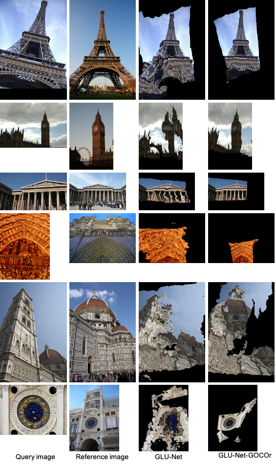
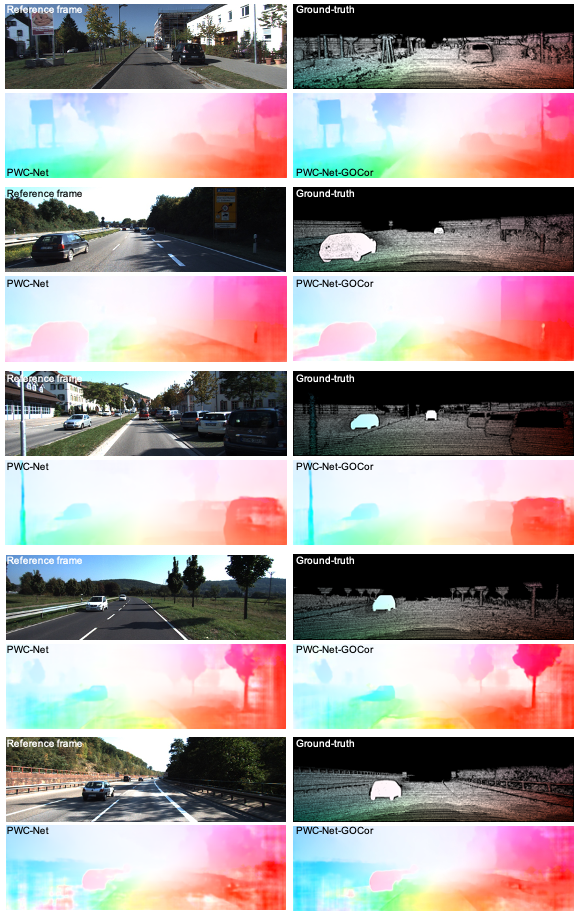
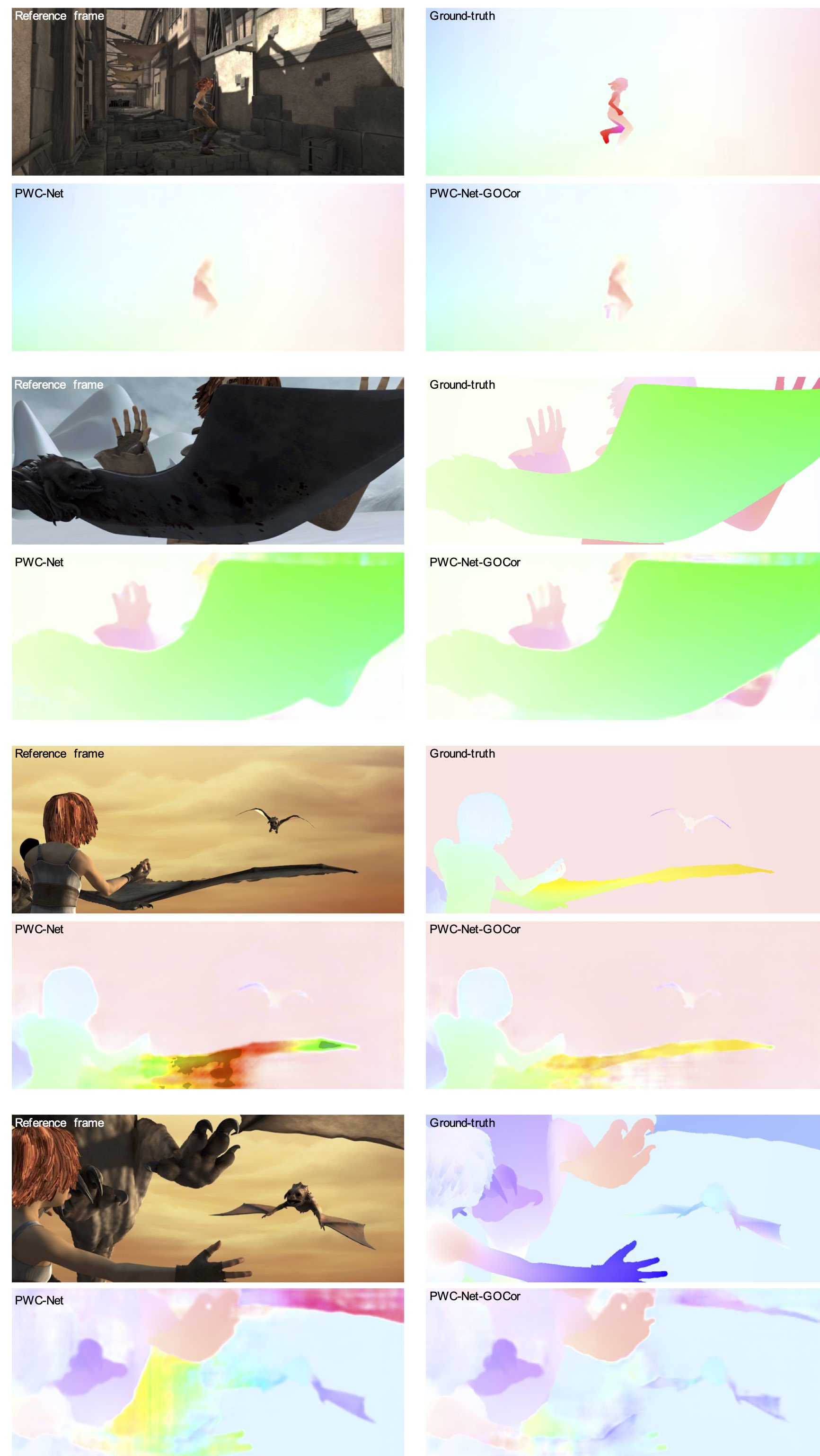
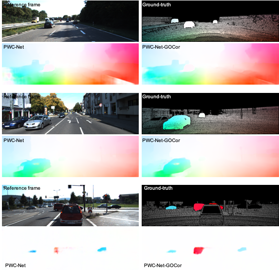
(a) ETH3D images

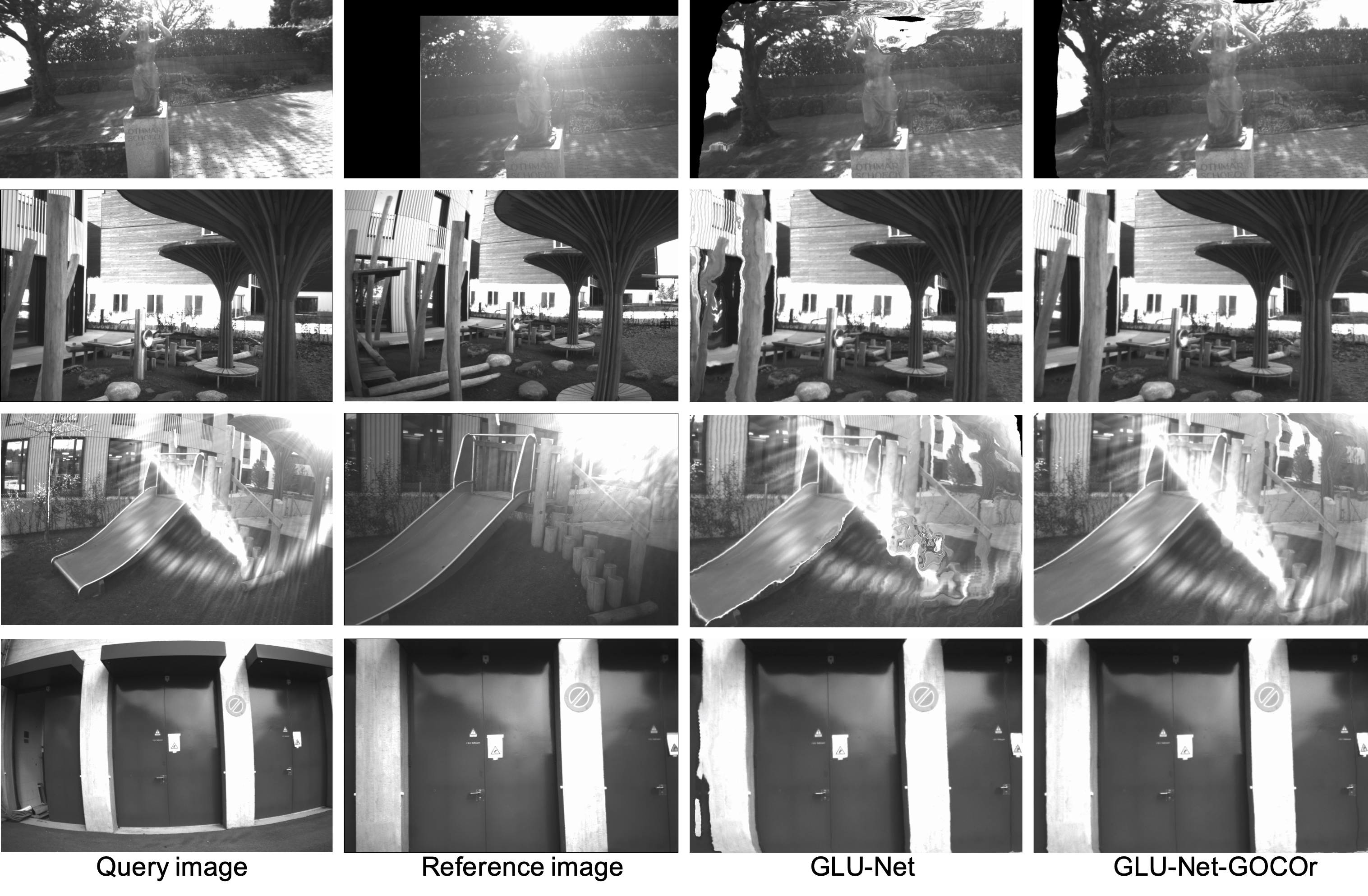
(b) Sintel-clean images

Figure 16: Qualitative examples of GLU-Net and GLU-Net-GOCor applied to images of (a) the ETH3D dataset and (b) the Sintel dataset, Clean pass. Both models are trained on the Dynamic dataset. In the case of the ETH3D images, we visualize the query images warped according to the flow fields estimated by the network. The warped query images should resemble the reference images. In the case of Sintel images, we plot directly the estimated flow field for each image pair.

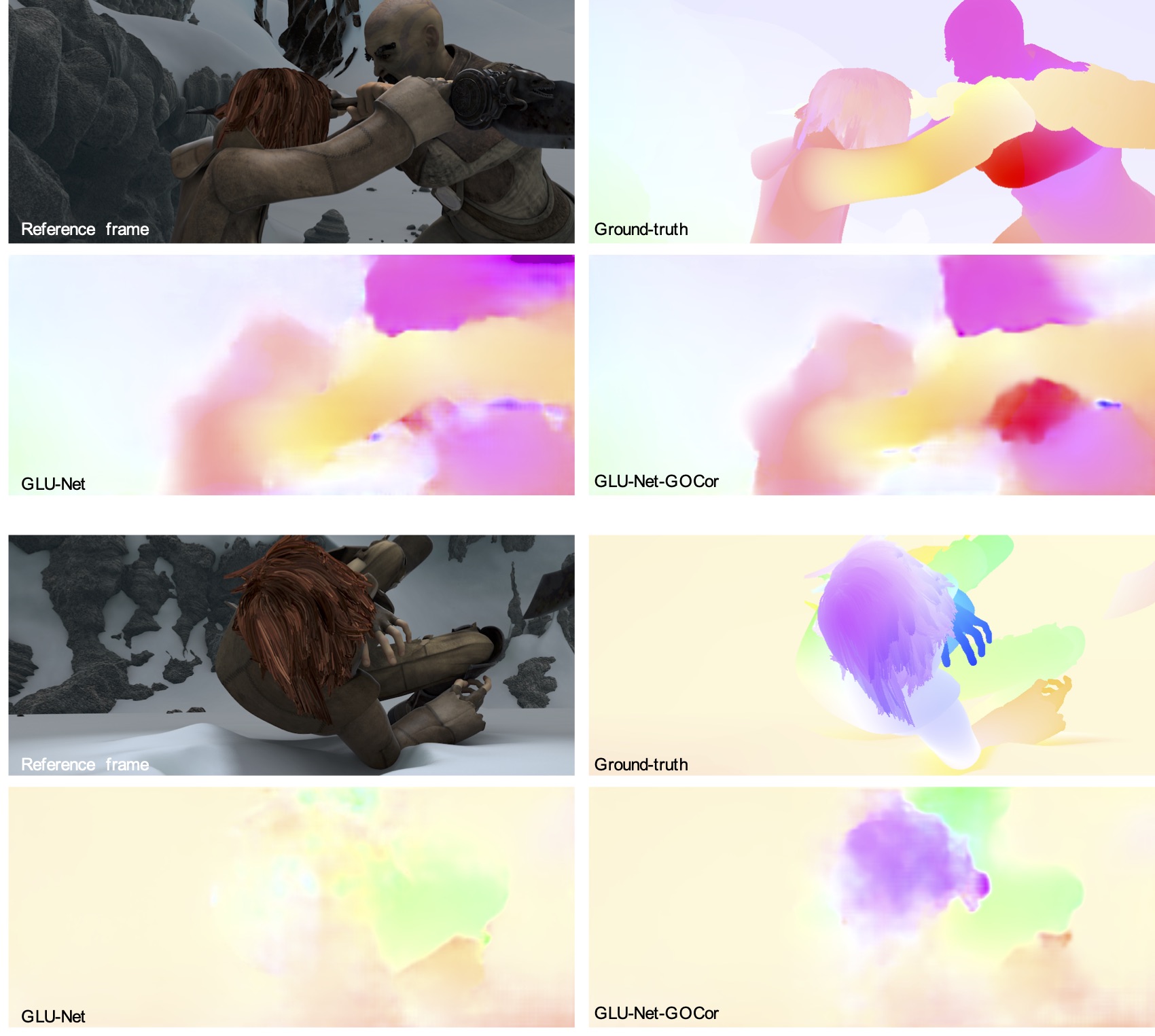
E.6 Results for smooth version of the reference loss

In Section 3.4, we defined our robust and learnable objective function for integrating reference frame information as $L_{\text{r}}(w;f^{r},\theta)=\left\|\sigma_{\eta}\big{(}\mathbf{C}(w,f^{r});\,v^{\scriptscriptstyle+},v^{\scriptscriptstyle-}\big{)}-y\right\|^{2}$ (eq. 4 of main paper), with $\sigma_{\eta}(\mathbf{C}(w,f^{r});v^{\scriptscriptstyle+}\!,v^{\scriptscriptstyle-})=\frac{v^{\scriptscriptstyle+}\!-v^{\scriptscriptstyle-}\!}{2}\!\left(\!\sqrt{\mathbf{C}(w,f^{r})^{2}+\eta^{2}}-\eta\right)+\frac{v^{\scriptscriptstyle+}\!+v^{\scriptscriptstyle-}\!}{2}\mathbf{C}(w,f^{r})$ (eq. 4 of main paper).

Here, setting $\eta>0$ enables to avoid the discontinuity in the derivative of $\sigma$ at $\varepsilon=0$. We analyze two different settings for $\eta$ when integrated in GLU-Net-GOCor. Specifically, in Table 14, we compare the results obtained by GLU-Net-GOCor on optical flow data, when setting $\eta=0$ or $\eta=0.1$. Both values obtain very similar results. Therefore, for simplicity and efficiency, we use $\eta=0$ in all other experiments.

Table 14: Comparison of different parametrisation for our robust loss formulation $L^{r}$. Both GLU-Net-GOCor are trained on the Dynamic dataset with three optimization iterations and evaluated with three and seven iterations for respectively the global-GOCor and the local-GOCor modules.

	KITTI-2012		KITTI-2015		Sintel Clean			Sintel Final
	AEPE $\downarrow$	F1 [%] $\downarrow$	AEPE $\downarrow$	F1 [%] $\downarrow$	AEPE $\downarrow$	PCK-1 [%] $\uparrow$	PCK-5 [%] $\uparrow$	AEPE $\downarrow$	PCK-1 [%] $\uparrow$	PCK-5 [%] $\uparrow$
GLU-Net	3.14	19.76	7.49	33.83	4.25	62.08	88.40	5.50	57.85	85.10
GLU-Net-GOCor, $\eta=0$	2.68	15.43	6.68	27.57	3.80	67.12	90.41	4.90	63.38	87.69
GLU-Net-GOCor, $\eta=0.1$	2.70	15.51	6.92	28.06	3.74	66.72	90.42	4.81	63.04	87.69

(A) 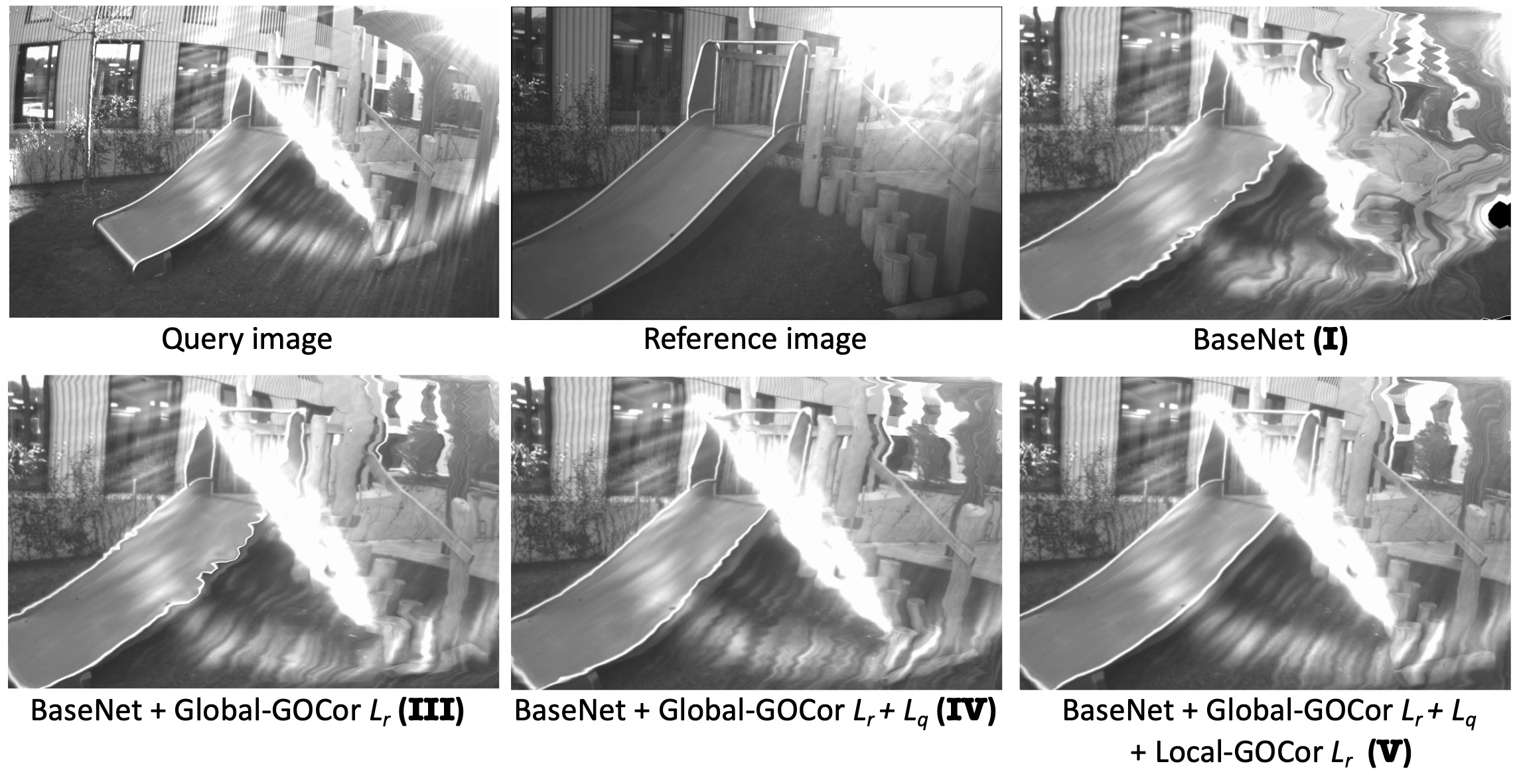(B)

Figure 17: Qualitative analysis of the different components of our approach, when the corresponding networks are applied to images of the ETH3D dataset. All models are trained on the Dynamic dataset. We visualize the query images warped according to the flow fields estimated by the networks. The warped query images should resemble the reference images.

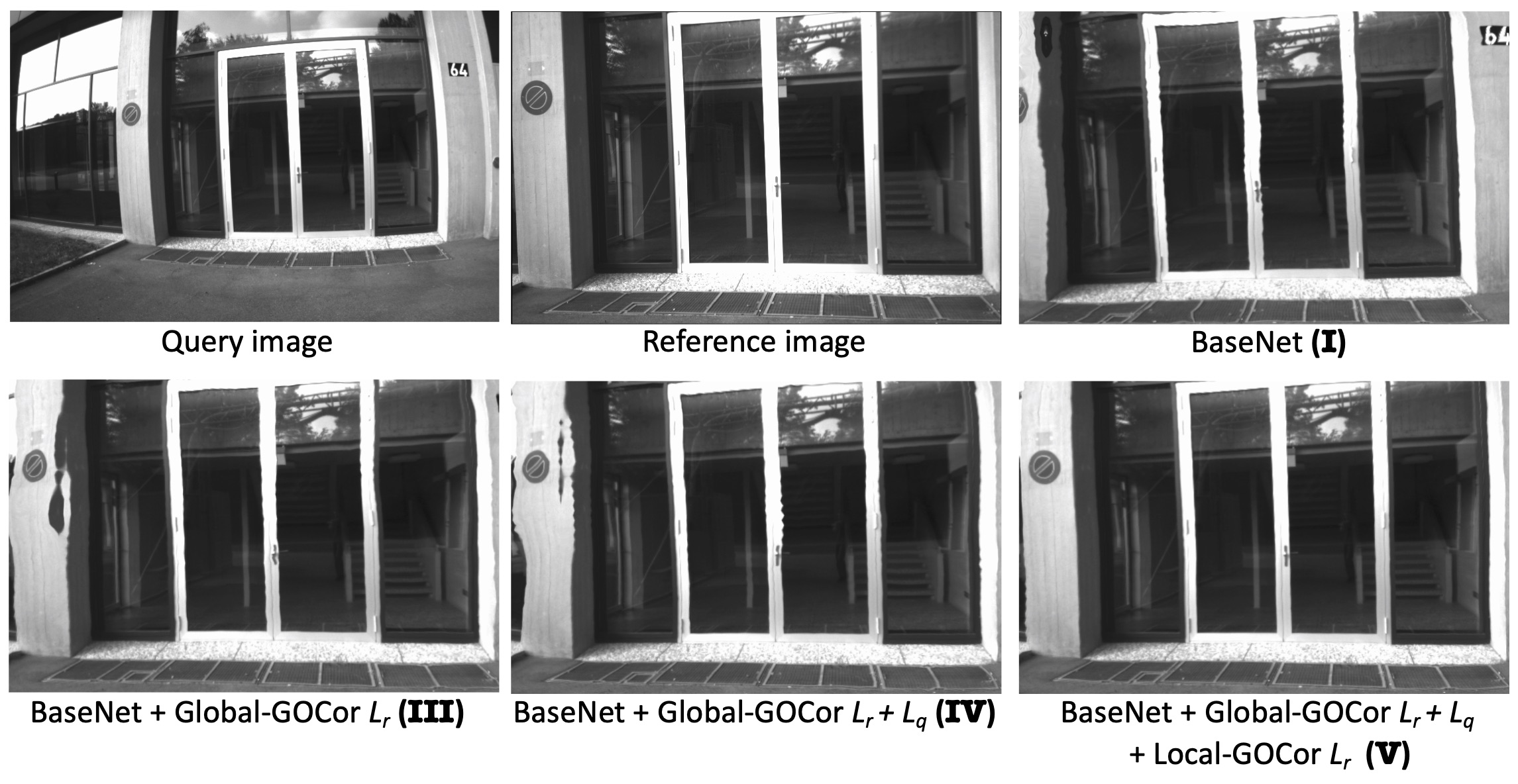
(A) KITTI-2015 (B) Sintel-clean

Figure 18: Qualitative analysis of the different components of our approach, when the corresponding networks are applied to images of the Sintel dataset, clean pass. All models are trained on the Dynamic dataset. We plot directly the estimated flow field for each image pair.

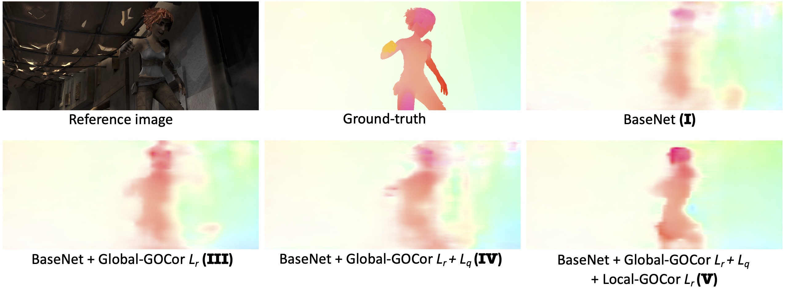
Appendix F Additional ablation study

For completeness, in Table 15, we provide a similar ablation study as that of the main paper, when BaseNet is trained on the Static data, instead of the Dynamic one. The same conclusions apply. We thus perform the additional ablative experiments when training all BaseNet variants on the Static data.

Qualitative ablation study: We visualize the quality of the estimated flow fields outputted by BaseNet (I), BaseNet + Global-GOCor $L_{r}$ (III), BaseNet + Global-GOCor $L_{r}+L_{q}$ (IV) and BaseNet + Global-GOCor $L_{r}+L_{q}$ + Local-GOCor $L_{r}$ (V) when applied to images of the ETH3D dataset and of optical flow datasets Sintel and KITTI in respectively Figures 17 and 18. Example (A) of Figure 17 shows the benefit of our global GOCor module as compared to the global feature correlation layer. Indeed, BaseNet does not manage to correctly capture the geometric transformation between the query and the reference images. On the other hand, thanks to our global GOCor module, BaseNet + Global-GOCor estimates a much more accurate transformation relating the frames. In example (B), we illustrate the gradual improvement from version (III) to (V). While introducing Global-GOCor with only the reference loss $L_{r}$ (version III) makes the estimated flow more stable than BaseNet, especially in the background, the representation of the slide object on the warped image is still shaky. Adding the query loss $L_{q}$ (version IV) smooths the estimated flow, and therefore the warped query image according to this flow. The later looks visually much better because of additional smoothness. Finally, further substituting the local feature correlation layers with our local GOCor module (version V) finishes to polish the result. The slide object in that case looks almost perfect and artifacts in the background are partially removed.

The impact of the query frame objective $L_{q}$ in our global GOCor module is further illustrated in example (A) of Figure 18. Introducing $L_{q}$ enables to smooth the estimated flow field and to remove part of the artifacts. Finally, the advantage of our local GOCor module as opposed to the local feature correlation layer is visualized in both examples of Figure 18. From version (IV) to (V), the local GOCor module can recover sharper motion boundaries and the estimated flow is generally more accurate. Moreover, remaining artifacts in the background are removed.

Comparison with post-processing method NC-Net: Here, we investigate the impact of post-processing method NC-Net [47] and show comparisons to BaseNet and our approach in Table 15. When trained on the Static dataset, including post-processing module NC-Net following the global correlation layer (version II) leads to better results than original version BaseNet (I) on the HPatches and the KITTI-2012 datasets. However, on the KITTI-2015 images, adding NC-Net results in worse performance. This is due to the fact that NC-Net uses correspondences with high confidences to support other uncertain neighboring matches. However, in the case of independently moving objects, neighboring matches can correspond to completely different motions, which breaks the assumption of the neighborhood consensus constraint used in NC-Net. Since it cannot cope with independently moving objects, NC-Net obtains worse results on KITTI-2015, which depicts dynamic scenes. This is contrary to HPatches which present planar scenes with homographies and to KITTI-2012, which is restricted to static scenes. This observation is also emphasized by the ablation study in Table 3 of the main paper, where BaseNet + NC-Net is trained on the Dynamic dataset. In that case, the performance of the resulting network is much worse than original BaseNet on all datasets. This is again due to the inability of NC-Net to handle moving objects, in that case, present in the training dataset. This shows the advantage of our method, which instead of applying 4D convolutions to post-process the correspondence volume, integrates them before the correlation operation itself.

Impact of objective function in the Local GOCor: In Table 15, we analyse the impact of both terms $L_{r},L_{q}$ of our objective function $L$ when used in our Local GOCor module. Comparing versions (V) and (VI), we found that adding the loss on the query frame $L_{\text{q}}$ (Sec 3.5) for Local-GOCor is harmful for its performance, particularly on the KITTI-datasets. Besides, adding the regularizer loss in the local GOCor level leads to longer training and inference run times. We therefore do not include it, our best version of BaseNet-GOCor resulting in (V).

Table 15: Ablation study. All networks are trained on the Static dataset. The GOCor modules are trained and evaluated with 3 steepest descent iterations.

		HP		KITTI-2012		KITTI-2015
		AEPE $\downarrow$	PCK-5 [%] $\uparrow$	AEPE $\downarrow$	F1 [%] $\downarrow$	AEPE $\downarrow$	F1 [%] $\downarrow$
I	BaseNet	26.73	65.30	4.95	42.49	11.52	61.90
II	BaseNet + NC-Net	24.59	66.62	5.00	39.80	12.44	62.96
III	BaseNet + Global-GOCor $L_{r}$	22.80	70.00	4.43	34.81	10.93	55.73
IV	BaseNet + Global-GOCor $L_{r}+L_{q}$	22.16	70.54	4.36	34.15	10.97	55.62
V	BaseNet + Global-GOCor $L_{r}+L_{q}$ + Local-GOCor $L_{r}$	22.00	74.80	4.02	31.24	9.92	50.54
VI	BaseNet + Global-GOCor $L_{r}+L_{q}$ + Local-GOCor $L_{r}+L_{q}$	21.96	75.26	4.24	33.43	10.20	53.53

Impact of number of training optimization iterations: Here, we investigate the influence of the number of training steepest descent iterations. We train multiple BaseNet-GOCor networks, gradually increasing the number of training optimization iterations within the global and the local GOCor modules. All networks are trained on the Static dataset. We evaluate all variants on the HPatches, KITTI and Sintel datasets and present the results in Table 16. We use the same number of optimization iteration during evaluation as during training. We additionally measure the inference run-time of each network, computed as the average over the 194 KITTI-2012 images on an NVIDIA Titan X GPU.

Training and evaluating with more steepest descent iterations consistently leads to better performances on all metrics and all datasets. It is also interesting to note that BaseNet + Global-GOCor without going through the optimizer (0 iteration) already outperforms the original BaseNet. In that case, the improvement is solely due to our powerful initialization $w^{0}$.

Nevertheless, the improvement in performance when increasing the number of optimization iterations comes at the expense of inference and training time. As a result, we trained all our GOCor modules with three iterations which presented a satisfactory trade-off between inference time and accuracy. Besides, it must also be noted that for time-critical applications, using a single optimization iteration for both local and global GOCor modules already leads to significant improvements over the standard feature correlation layer.

Table 16: Analysis of the number of training optimization iterations. Both Local-GOCor and Global-GOCor layers are trained and evaluated with the same number of iterations. All networks are trained on the Static dataset.

	KITTI-2012			HP			Sintel-clean
	Run-time [ms]	AEPE $\downarrow$	F1 [%] $\downarrow$	AEPE $\downarrow$	PCK-1 [%]$\uparrow$	PCK-5 [%] $\uparrow$	AEPE $\downarrow$	PCK-1 [%] $\uparrow$	PCK-5 [%] $\uparrow$
BaseNet	63.20	4.95	42.49	26.73	12.02	65.30	7.78	12.46	74.52
BaseNet-GOCor, optim-iter = 0	66.80	4.87	37.42	26.47	16.40	66.42	6.94	27.63	77.20
BaseNet-GOCor, optim-iter = 1	70.52	4.18	32.95	21.91	20.73	72.82	6.49	31.03	79.87
BaseNet-GOCor, optim-iter = 3	82.42	4.02	31.24	22.00	23.68	74.80	6.32	33.81	80.72
BaseNet-GOCor, optim-iter = 5	94.85	3.83	29.14	20.68	25.99	76.88	6.34	38.10	80.91

Impact of performing global correlation with interchanging query and reference features: We also experimented with interchanging the query and reference frames at the global level, and then fusing the two resulting GOCor correspondence volumes before passing them to the flow estimation decoder. However, we only observed marginal improvements. e.g., on KITTI-2015 it obtains an EPE of 11.07 and an F1 of 54.68% compared to 10.97 EPE and 55.62% F1 for the baseline BaseNet + Global-GOCor $L_{r}+L_{q}$ (IV). Considering that computing the GOCor correspondence volume twice increases the inference time of the model and the limited improvement of performance brought by fusing the two resulting correspondence volumes, we did not include this alternative in the final model.

Impact of filter initializer $w^{0}$: As detailed in Sec. B, we introduced several versions of our filter initializer module. Here, we train BaseNet with standard local feature correlation layers and our Global-GOCor module (using both our loss on the reference and on the query images) integrated in place of the global correlation layer. We experiment with different variants of the initializer and present the corresponding evaluation results in Table 17. The version ZeroInitializer initializes $w^{0}$ to a zero tensor. Compared to all others, this initialization lacks accuracy for the final network, particularly on the optical flow datasets. In the SimpleInitializer versions which do not include global context information, adding more flexibility in the form of a learnt vector does not seem to help. However, in the case where context information is included, compared to ContextAwareInitializer, the Flexible variant significantly gains from increased flexibility. Initializer module Flexible-ContextAwareInitializer appears to be the best alternative for our Global-GOCor module.

Table 17: Analysis of the impact of the initializer for the Global-GOCor. All networks are trained on the Static with three optimization iterations. They are evaluated with the same number of iterations.

	HP			KITTI-2012		Sintel-clean
	AEPE $\downarrow$	PCK-1 [%] $\uparrow$	PCK-5 [%] $\uparrow$	AEPE $\downarrow$	F1 [%] $\downarrow$	AEPE $\downarrow$	PCK-1 [%] $\uparrow$	PCK-5 [%] $\uparrow$
BaseNet + Global-GOCor, ZeroInitializer	23.22	14.05	67.53	4.77	38.67	7.56	14.94	74.96
BaseNet + Global-GOCor, SimpleInitializer	24.69	13.17	66.82	4.81	37.86	7.32	20.31	76.12
BaseNet + Global-GOCor, Flexible-SimpleInitializer	25.53	12.82	66.97	4.83	38.71	7.30	20.48	76.24
BaseNet + Global-GOCor, ContextAwareInitializer	25.13	15.01	67.14	4.87	39.14	7.43	19.19	75.60
BaseNet + Global-GOCor, Flexible-ContextAwareInitializer	22.16	17.03	70.54	4.36	34.15	7.21	20.68	77.09

References

- [1] Sameer Agarwal, Yasutaka Furukawa, Noah Snavely, Ian Simon, Brian Curless, Steven M. Seitz, and Richard Szeliski. Building rome in a day. Commun. ACM, 54(10):105–112, 2011.
- [2] Simon Baker, Daniel Scharstein, J. P. Lewis, Stefan Roth, Michael J. Black, and Richard Szeliski. A database and evaluation methodology for optical flow. International Journal of Computer Vision, 92(1):1–31, 2011.
- [3] Vassileios Balntas, Karel Lenc, Andrea Vedaldi, and Krystian Mikolajczyk. Hpatches: A benchmark and evaluation of handcrafted and learned local descriptors. In 2017 IEEE Conference on Computer Vision and Pattern Recognition, CVPR 2017, Honolulu, HI, USA, July 21-26, 2017, pages 3852–3861, 2017.
- [4] Luca Bertinetto, João F. Henriques, Philip H. S. Torr, and Andrea Vedaldi. Meta-learning with differentiable closed-form solvers. In 7th International Conference on Learning Representations, ICLR 2019, New Orleans, LA, USA, May 6-9, 2019, 2019.
- [5] Goutam Bhat, Martin Danelljan, Luc Van Gool, and Radu Timofte. Learning discriminative model prediction for tracking. In 2019 IEEE/CVF International Conference on Computer Vision, ICCV 2019, Seoul, Korea (South), October 27 - November 2, 2019, pages 6181–6190. IEEE, 2019.
- [6] Goutam Bhat, Felix Järemo Lawin, Martin Danelljan, Andreas Robinson, Michael Felsberg, Luc Van Gool, and Radu Timofte. Learning what to learn for video object segmentation. In European Conference on Computer Vision ECCV, 2020.
- [7] Thomas Brox and Jitendra Malik. Large displacement optical flow: Descriptor matching in variational motion estimation. IEEE Trans. Pattern Anal. Mach. Intell., 33(3):500–513, 2011.
- [8] Daniel J. Butler, Jonas Wulff, Garrett B. Stanley, and Michael J. Black. A naturalistic open source movie for optical flow evaluation. In Computer Vision - ECCV 2012 - 12th European Conference on Computer Vision, Florence, Italy, October 7-13, 2012, Proceedings, Part VI, pages 611–625, 2012.
- [9] K. Chatfield, K. Simonyan, A. Vedaldi, and A. Zisserman. Return of the devil in the details: Delving deep into convolutional nets. In BMVC, 2014.
- [10] Jianchun Chen, Lingjing Wang, Xiang Li, and Yi Fang. Arbicon-net: Arbitrary continuous geometric transformation networks for image registration. In Hanna M. Wallach, Hugo Larochelle, Alina Beygelzimer, Florence d’Alché-Buc, Emily B. Fox, and Roman Garnett, editors, Advances in Neural Information Processing Systems 32: Annual Conference on Neural Information Processing Systems 2019, NeurIPS 2019, 8-14 December 2019, Vancouver, BC, Canada, pages 3410–3420, 2019.
- [11] Yuhua Chen, Jordi Pont-Tuset, Alberto Montes, and Luc Van Gool. Blazingly fast video object segmentation with pixel-wise metric learning. In Proceedings of the IEEE Conference on Computer Vision and Pattern Recognition, pages 1189–1198, 2018.
- [12] Zhuoyuan Chen, Xun Sun, Liang Wang, Yinan Yu, and Chang Huang. A deep visual correspondence embedding model for stereo matching costs. In 2015 IEEE International Conference on Computer Vision, ICCV 2015, Santiago, Chile, December 7-13, 2015, pages 972–980, 2015.
- [13] Christopher Bongsoo Choy, JunYoung Gwak, Silvio Savarese, and Manmohan Krishna Chandraker. Universal correspondence network. In Advances in Neural Information Processing Systems 29: Annual Conference on Neural Information Processing Systems 2016, December 5-10, 2016, Barcelona, Spain, pages 2406–2414, 2016.
- [14] Marius Cordts, Mohamed Omran, Sebastian Ramos, Timo Rehfeld, Markus Enzweiler, Rodrigo Benenson, Uwe Franke, Stefan Roth, and Bernt Schiele. The cityscapes dataset for semantic urban scene understanding. In Proc. of the IEEE Conference on Computer Vision and Pattern Recognition (CVPR), 2016.
- [15] Daniel DeTone, Tomasz Malisiewicz, and Andrew Rabinovich. Deep image homography estimation. CoRR, abs/1606.03798, 2016.
- [16] Alexey Dosovitskiy, Philipp Fischer, Eddy Ilg, Philip Häusser, Caner Hazirbas, Vladimir Golkov, Patrick van der Smagt, Daniel Cremers, and Thomas Brox. Flownet: Learning optical flow with convolutional networks. In 2015 IEEE International Conference on Computer Vision, ICCV 2015, Santiago, Chile, December 7-13, 2015, pages 2758–2766, 2015.
- [17] Andreas Geiger, Philip Lenz, Christoph Stiller, and Raquel Urtasun. Vision meets robotics: The kitti dataset. I. J. Robotic Res., 32(11):1231–1237, 2013.
- [18] Berthold K. P. Horn and Brian G. Schunck. "determining optical flow": A retrospective. Artif. Intell., 59(1-2):81–87, 1993.
- [19] Yuan-Ting Hu, Jia-Bin Huang, and Alexander G Schwing. Videomatch: Matching based video object segmentation. In European Conference on Computer Vision, pages 56–73. Springer, 2018.
- [20] Shuaiyi Huang, Qiuyue Wang, Songyang Zhang, Shipeng Yan, and Xuming He. Dynamic context correspondence network for semantic alignment. In 2019 IEEE/CVF International Conference on Computer Vision, ICCV 2019, Seoul, Korea (South), October 27 - November 2, 2019, pages 2010–2019. IEEE, 2019.
- [21] Tak-Wai Hui, Xiaoou Tang, and Chen Change Loy. Liteflownet: A lightweight convolutional neural network for optical flow estimation. In 2018 IEEE Conference on Computer Vision and Pattern Recognition, CVPR 2018, Salt Lake City, UT, USA, June 18-22, 2018, pages 8981–8989, 2018.
- [22] Tak-Wai Hui, Xiaoou Tang, and Chen Change Loy. A Lightweight Optical Flow CNN - Revisiting Data Fidelity and Regularization. 2020.
- [23] Andrey Ignatov, Nikolay Kobyshev, Radu Timofte, Kenneth Vanhoey, and Luc Van Gool. Dslr-quality photos on mobile devices with deep convolutional networks. In IEEE International Conference on Computer Vision, ICCV 2017, Venice, Italy, October 22-29, 2017, pages 3297–3305, 2017.
- [24] Eddy Ilg, Nikolaus Mayer, Tonmoy Saikia, Margret Keuper, Alexey Dosovitskiy, and Thomas Brox. Flownet 2.0: Evolution of optical flow estimation with deep networks. In 2017 IEEE Conference on Computer Vision and Pattern Recognition, CVPR 2017, Honolulu, HI, USA, July 21-26, 2017, pages 1647–1655. IEEE Computer Society, 2017.
- [25] Joel Janai, Fatma Güney, Aseem Behl, and Andreas Geiger. Computer vision for autonomous vehicles: Problems, datasets and state-of-the-art. CoRR, abs/1704.05519, 2017.
- [26] Sangryul Jeon, Seungryong Kim, Dongbo Min, and Kwanghoon Sohn. PARN: pyramidal affine regression networks for dense semantic correspondence. In Computer Vision - ECCV 2018 - 15th European Conference, Munich, Germany, September 8-14, 2018, Proceedings, Part VI, pages 355–371, 2018.
- [27] Xu Jia, Bert De Brabandere, Tinne Tuytelaars, and Luc Van Gool. Dynamic filter networks. In Advances in Neural Information Processing Systems 29: Annual Conference on Neural Information Processing Systems 2016, December 5-10, 2016, Barcelona, Spain, pages 667–675, 2016.
- [28] Seungryong Kim, Stephen Lin, Sangryul Jeon, Dongbo Min, and Kwanghoon Sohn. Recurrent transformer networks for semantic correspondence. In Advances in Neural Information Processing Systems 31: Annual Conference on Neural Information Processing Systems 2018, NeurIPS 2018, 3-8 December 2018, Montréal, Canada., pages 6129–6139, 2018.
- [29] Seungryong Kim, Dongbo Min, Bumsub Ham, Stephen Lin, and Kwanghoon Sohn. FCSS: fully convolutional self-similarity for dense semantic correspondence. IEEE Trans. Pattern Anal. Mach. Intell., 41(3):581–595, 2019.
- [30] Seungryong Kim, Dongbo Min, Somi Jeong, Sunok Kim, Sangryul Jeon, and Kwanghoon Sohn. Semantic attribute matching networks. In IEEE Conference on Computer Vision and Pattern Recognition, CVPR 2019, Long Beach, CA, USA, June 16-20, 2019, pages 12339–12348, 2019.
- [31] Zakaria Laskar, Iaroslav Melekhov, Hamed R. Tavakoli, Juha Ylioinas, and Juho Kannala. Geometric image correspondence verification by dense pixel matching. CoRR, abs/1904.06882, 2019.
- [32] Kwonjoon Lee, Subhransu Maji, Avinash Ravichandran, and Stefano Soatto. Meta-learning with differentiable convex optimization. In IEEE Conference on Computer Vision and Pattern Recognition, CVPR 2019, Long Beach, CA, USA, June 16-20, 2019, pages 10657–10665, 2019.
- [33] Shuda Li, Kai Han, Theo W. Costain, Henry Howard-Jenkins, and Victor Prisacariu. Correspondence networks with adaptive neighbourhood consensus. CoRR, abs/2003.12059, 2020.
- [34] Zhengqi Li and Noah Snavely. Megadepth: Learning single-view depth prediction from internet photos. In 2018 IEEE Conference on Computer Vision and Pattern Recognition, CVPR 2018, Salt Lake City, UT, USA, June 18-22, 2018, pages 2041–2050, 2018.
- [35] Zhengfa Liang, Yiliu Feng, Yulan Guo, Hengzhu Liu, Wei Chen, Linbo Qiao, Li Zhou, and Jianfeng Zhang. Learning for disparity estimation through feature constancy. In 2018 IEEE Conference on Computer Vision and Pattern Recognition, CVPR 2018, Salt Lake City, UT, USA, June 18-22, 2018, pages 2811–2820, 2018.
- [36] Tsung-Yi Lin, Michael Maire, Serge J. Belongie, Lubomir D. Bourdev, Ross B. Girshick, James Hays, Pietro Perona, Deva Ramanan, Piotr Dollár, and C. Lawrence Zitnick. Microsoft COCO: common objects in context. CoRR, abs/1405.0312, 2014.
- [37] Ce Liu, Jenny Yuen, and Antonio Torralba. SIFT flow: Dense correspondence across scenes and its applications. IEEE Trans. Pattern Anal. Mach. Intell., 33(5):978–994, 2011.
- [38] Jinlu Liu and Yongqiang Qin. Prototype refinement network for few-shot segmentation. CoRR, abs/2002.03579, 2020.
- [39] Iaroslav Melekhov, Aleksei Tiulpin, Torsten Sattler, Marc Pollefeys, Esa Rahtu, and Juho Kannala. DGC-Net: Dense geometric correspondence network. In Proceedings of the IEEE Winter Conference on Applications of Computer Vision (WACV), 2019.
- [40] Vinod Nair and Geoffrey E. Hinton. Rectified linear units improve restricted boltzmann machines. In Proceedings of the 27th International Conference on Machine Learning (ICML-10), June 21-24, 2010, Haifa, Israel, pages 807–814, 2010.
- [41] Jorge Nocedal and Stephen J. Wright. Numerical Optimization. Springer, New York, NY, USA, second edition, 2006.
- [42] Seoung Wug Oh, Joon-Young Lee, Ning Xu, and Seon Joo Kim. Video object segmentation using space-time memory networks. Proceedings of the IEEE International Conference on Computer Vision, 2019.
- [43] Jiahao Pang, Wenxiu Sun, Jimmy S. J. Ren, Chengxi Yang, and Qiong Yan. Cascade residual learning: A two-stage convolutional neural network for stereo matching. CoRR, abs/1708.09204, 2017.
- [44] Anurag Ranjan and Michael J. Black. Optical flow estimation using a spatial pyramid network. In 2017 IEEE Conference on Computer Vision and Pattern Recognition, CVPR 2017, Honolulu, HI, USA, July 21-26, 2017, pages 2720–2729, 2017.
- [45] Ignacio Rocco, Relja Arandjelovic, and Josef Sivic. Convolutional neural network architecture for geometric matching. In 2017 IEEE Conference on Computer Vision and Pattern Recognition, CVPR 2017, Honolulu, HI, USA, July 21-26, 2017, pages 39–48, 2017.
- [46] Ignacio Rocco, Relja Arandjelovic, and Josef Sivic. End-to-end weakly-supervised semantic alignment. In 2018 IEEE Conference on Computer Vision and Pattern Recognition, CVPR 2018, Salt Lake City, UT, USA, June 18-22, 2018, pages 6917–6925, 2018.
- [47] Ignacio Rocco, Mircea Cimpoi, Relja Arandjelovic, Akihiko Torii, Tomás Pajdla, and Josef Sivic. Neighbourhood consensus networks. In Advances in Neural Information Processing Systems 31: Annual Conference on Neural Information Processing Systems 2018, NeurIPS 2018, 3-8 December 2018, Montréal, Canada., pages 1658–1669, 2018.
- [48] Paul-Edouard Sarlin, Daniel DeTone, Tomasz Malisiewicz, and Andrew Rabinovich. Superglue: Learning feature matching with graph neural networks. In 2020 IEEE/CVF Conference on Computer Vision and Pattern Recognition, CVPR 2020, Seattle, WA, USA, June 13-19, 2020, pages 4937–4946, 2020.
- [49] Johannes L. Schönberger and Jan-Michael Frahm. Structure-from-motion revisited. In 2016 IEEE Conference on Computer Vision and Pattern Recognition, CVPR 2016, Las Vegas, NV, USA, June 27-30, 2016, pages 4104–4113, 2016.
- [50] Johannes L. Schönberger, Marc Pollefeys, Andreas Geiger, and Torsten Sattler. Semantic visual localization. In 2018 IEEE Conference on Computer Vision and Pattern Recognition, CVPR 2018, Salt Lake City, UT, USA, June 18-22, 2018, pages 6896–6906. IEEE Computer Society, 2018.
- [51] Thomas Schöps, Johannes L. Schönberger, Silvano Galliani, Torsten Sattler, Konrad Schindler, Marc Pollefeys, and Andreas Geiger. A multi-view stereo benchmark with high-resolution images and multi-camera videos. In 2017 IEEE Conference on Computer Vision and Pattern Recognition, CVPR 2017, Honolulu, HI, USA, July 21-26, 2017, pages 2538–2547, 2017.
- [52] Xi Shen, François Darmon, Alexei A Efros, and Mathieu Aubry. Ransac-flow: generic two-stage image alignment. In 16th European Conference on Computer Vision, 2020.
- [53] Jonathan R Shewchuk. An introduction to the conjugate gradient method without the agonizing pain. Technical report, USA, 1994.
- [54] Karen Simonyan and Andrew Zisserman. Two-stream convolutional networks for action recognition in videos. CoRR, abs/1406.2199, 2014.
- [55] Deqing Sun, Xiaodong Yang, Ming-Yu Liu, and Jan Kautz. Pwc-net: Cnns for optical flow using pyramid, warping, and cost volume. In 2018 IEEE Conference on Computer Vision and Pattern Recognition, CVPR 2018, Salt Lake City, UT, USA, June 18-22, 2018, pages 8934–8943, 2018.
- [56] Deqing Sun, Xiaodong Yang, Ming-Yu Liu, and Jan Kautz. Models matter, so does training: An empirical study of cnns for optical flow estimation. IEEE transactions on pattern analysis and machine intelligence, 2019.
- [57] Hajime Taira, Masatoshi Okutomi, Torsten Sattler, Mircea Cimpoi, Marc Pollefeys, Josef Sivic, Tomás Pajdla, and Akihiko Torii. Inloc: Indoor visual localization with dense matching and view synthesis. In 2018 IEEE Conference on Computer Vision and Pattern Recognition, CVPR 2018, Salt Lake City, UT, USA, June 18-22, 2018, pages 7199–7209. IEEE Computer Society, 2018.
- [58] Tatsunori Taniai, Sudipta N. Sinha, and Yoichi Sato. Joint recovery of dense correspondence and cosegmentation in two images. In 2016 IEEE Conference on Computer Vision and Pattern Recognition, CVPR 2016, Las Vegas, NV, USA, June 27-30, 2016, pages 4246–4255, 2016.
- [59] Prune Truong, Martin Danelljan, and Radu Timofte. GLU-Net: Global-local universal network for dense flow and correspondences. In 2020 IEEE Conference on Computer Vision and Pattern Recognition, CVPR 2020, 2020.
- [60] Jack Valmadre, Luca Bertinetto, João F. Henriques, Andrea Vedaldi, and Philip H. S. Torr. End-to-end representation learning for correlation filter based tracking. In 2017 IEEE Conference on Computer Vision and Pattern Recognition, CVPR 2017, Honolulu, HI, USA, July 21-26, 2017, pages 5000–5008, 2017.
- [61] Paul Voigtlaender and Bastian Leibe. Feelvos: Fast end-to-end embedding learning for video object segmentation. In IEEE Conference on Computer Vision and Pattern Recognition (CVPR), 2019.
- [62] Kaixin Wang, Jun Hao Liew, Yingtian Zou, Daquan Zhou, and Jiashi Feng. Panet: Few-shot image semantic segmentation with prototype alignment. In 2019 IEEE/CVF International Conference on Computer Vision, ICCV 2019, Seoul, Korea (South), October 27 - November 2, 2019, pages 9196–9205, 2019.
- [63] Taihong Xiao, Jinwei Yuan, Deqing Sun, Qifei Wang, Xin-Yu Zhang, Kehan Xu, and Ming-Hsuan Yang. Learnable cost volume using the cayley representation. CoRR, abs/2007.11431, 2020.
- [64] Gengshan Yang and Deva Ramanan. Volumetric correspondence networks for optical flow. In Hanna M. Wallach, Hugo Larochelle, Alina Beygelzimer, Florence d’Alché-Buc, Emily B. Fox, and Roman Garnett, editors, Advances in Neural Information Processing Systems 32: Annual Conference on Neural Information Processing Systems 2019, NeurIPS 2019, 8-14 December 2019, Vancouver, BC, Canada, pages 793–803, 2019.
- [65] Yinda Zhang, Sameh Khamis, Christoph Rhemann, Julien P. C. Valentin, Adarsh Kowdle, Vladimir Tankovich, Michael Schoenberg, Shahram Izadi, Thomas A. Funkhouser, and Sean Ryan Fanello. Activestereonet: End-to-end self-supervised learning for active stereo systems. In Computer Vision - ECCV 2018 - 15th European Conference, Munich, Germany, September 8-14, 2018, Proceedings, Part VIII, pages 802–819, 2018.
- [66] Bolei Zhou, Hang Zhao, Xavier Puig, Tete Xiao, Sanja Fidler, Adela Barriuso, and Antonio Torralba. Semantic understanding of scenes through the ADE20K dataset. Int. J. Comput. Vis., 127(3):302–321, 2019.
- [67] Luisa M. Zintgraf, Kyriacos Shiarlis, Vitaly Kurin, Katja Hofmann, and Shimon Whiteson. Fast context adaptation via meta-learning. In Proceedings of the 36th International Conference on Machine Learning, ICML 2019, 9-15 June 2019, Long Beach, California, USA, pages 7693–7702, 2019.