Convex Calibrated Surrogates for the Multi-Label F-Measure

Abstract

The $F$-measure is a widely used performance measure for multi-label classification, where multiple labels can be active in an instance simultaneously (e.g. in image tagging, multiple tags can be active in any image). In particular, the $F$-measure explicitly balances recall (fraction of active labels predicted to be active) and precision (fraction of labels predicted to be active that are actually so), both of which are important in evaluating the overall performance of a multi-label classifier. As with most discrete prediction problems, however, directly optimizing the $F$-measure is computationally hard. In this paper, we explore the question of designing convex surrogate losses that are calibrated for the $F$-measure – specifically, that have the property that minimizing the surrogate loss yields (in the limit of sufficient data) a Bayes optimal multi-label classifier for the $F$-measure. We show that the $F$-measure for an $s$-label problem, when viewed as a $2^{s}\times 2^{s}$ loss matrix, has rank at most $s^{2}+1$, and apply a result of Ramaswamy et al. (2014) to design a family of convex calibrated surrogates for the $F$-measure. The resulting surrogate risk minimization algorithms can be viewed as decomposing the multi-label $F$-measure learning problem into $s^{2}+1$ binary class probability estimation problems. We also provide a quantitative regret transfer bound for our surrogates, which allows any regret guarantees for the binary problems to be transferred to regret guarantees for the overall $F$-measure problem, and discuss a connection with the algorithm of Dembczynski et al. (2013). Our experiments confirm our theoretical findings.

1 Introduction

The $F_{\beta}$-measure is a widely used performance measure for multi-label classification (MLC) problems. In particular, in an MLC problem, multiple labels can be active in an instance simultaneously; a good example is that of image tagging, where several tags (such as sky, sand, water) can be active in the same image. In such problems, when evaluating the performance of a classifier on a particular instance, it is important to balance the recall of the classifier on the given instance, i.e. the fraction of active labels for that instance that are correctly predicted as such, and the precision of the classifier on the instance, i.e. the fraction of labels predicted to be active for that instance that are actually so. The $F_{\beta}$-measure accomplishes this by taking the (possibly weighted) harmonic mean of these two quantities.

Unfortunately, as with most discrete prediction problems, optimizing the $F_{\beta}$-measure directly during training is computationally hard. Consequently, one generally settles for some form of approximation. One approach is to simply treat the labels as independent, and train a separate binary classifier for each label; this is sometimes referred to as the binary relevance (BR) approach. Of course, this ignores the fact that labels can have correlations among them (e.g. sky and cloud may be more likely to co-occur than sky and computer). Several other approaches have been proposed in recent years (Dembczynski et al., 2013; Koyejo et al., 2015; Wu & Zhou, 2017; Pillai et al., 2017).

In this paper, we turn to the theory of convex calibrated surrogate losses – which has yielded convex risk minimization algorithms for several other discrete prediction problems in recent years (Bartlett et al., 2006; Zhang, 2004b; Tewari & Bartlett, 2007; Steinwart, 2007; Duchi et al., 2010; Gao & Zhou, 2013; Ramaswamy et al., 2014, 2015) – to design principled surrogate risk minimization algorithms for the multi-label $F_{\beta}$-measure. In particular, for an MLC problem with $s$ tags, the total number of possible labelings of an instance is $2^{s}$ (each tag can be active or inactive). Viewing the $F_{\beta}$-measure as (one minus) a $2^{s}\times 2^{s}$ loss matrix, we show that this matrix has rank at most $s^{2}+1$, and apply the results of Ramaswamy et al. (2014) to design an output coding scheme that reduces the $F_{\beta}$ learning problem to a set of $s^{2}+1$ binary class probability estimation (CPE) problems. By using a suitable binary surrogate risk minimization algorithm (such as binary logistic regression) for these binary problems, we effectively construct a $(s^{2}+1)$-dimensional convex calibrated surrogate loss for the $F_{\beta}$-measure. We also give a quantitative regret transfer bound for the constructed surrogate, which allows us to transfer any regret guarantees for the binary subproblems to guarantees on $F_{\beta}$-regret for the overall MLC problem. In particular, this means that using a consistent learner for the binary problems yields a consistent learner for the MLC problem (whose $F_{\beta}$-regret goes to zero as the training sample size increases).

Our algorithm is related to the plug-in algorithm of Dembczynski et al. (2013), which also estimates $s^{2}+1$ statistics of the underlying distribution. Dembczynski et al. (2013) estimate these statistics by reducing the $F_{\beta}$ maximization problem to $s$ multiclass CPE problems, each with at most $s+1$ classes (plus one binary CPE problem); we do so by reducing the problem to $s^{2}+1$ binary CPE problems. As we show, both algorithms effectively estimate the same $s^{2}+1$ statistics, and indeed, both perform similarly in experiments. Interestingly, the algorithm of Dembczynski et al. (2013), while motivated primarily by the plug-in approach, can also be viewed as minimizing a certain convex calibrated surrogate loss (different from ours); conversely, our algorithm, while motivated primarily by the convex calibrated surrogates approach, can also be viewed as a plug-in algorithm. Our study brings out interesting connections between the two approaches; in addition, to the best our knowledge, our analysis is the first to provide a quantitative regret transfer bound for calibrated surrogates for the $F_{\beta}$-measure.

Organization. Section 2 discusses related work. Section 3 gives preliminaries and background. Section 4 gives our convex calibrated surrogates for the $F_{\beta}$-measure; Section 5 provides a regret transfer bound for them. Section 6 discusses the relationship with the plug-in algorithm of Dembczynski et al. (2013). Section 7 summarizes our experiments.

2 Related Work

There has been much work on multi-label learning, learning with the $F_{\beta}$-measure, and convex calibrated surrogates. Below we briefly discuss work that is most related to our study. For detailed surveys on multi-label learning, we refer the reader to Zhang & Zhou (2014) and Pillai et al. (2017).

Bayes optimal multi-label classifiers. In an elegant study, Dembczynski et al. (2011) studied in detail the form of a Bayes optimal multi-label classifier for the $F_{1}$-measure. In particular, they showed that, for an $s$-label MLC problem, given a certain set of $s^{2}+1$ statistics of the true conditional label distribution (distribution over $2^{s}$ labelings), one can compute a Bayes optimal classifier for the $F_{1}$-measure in $O(s^{3})$ time. Their result extends to general $F_{\beta}$-measures. Bayes optimal classifiers have also been studied for other MLC performance measures, such as Hamming loss and subset 0-1 loss (Dembczynski et al., 2010).

Consistent algorithms for multi-label learning. Dembczynski et al. (2013) extended and operationalized the results of Dembczynski et al. (2011) by providing a consistent plug-in MLC algorithm for the $F_{\beta}$-measure. Specifically, they showed that the $s^{2}+1$ statistics of the conditional label distribution needed to compute a Bayes optimal classifier can be estimated via $s$ multiclass CPE problems, each with at most $s+1$ classes, plus one binary CPE problem; the statistics estimated by solving these CPE problems can then be plugged into the $O(s^{3})$-time procedure of Dembczynski et al. (2011) to produce a consistent plug-in algorithm termed the exact F-measure plug-in (EFP) algorithm. Consistent learning algorithms have also been studied for other multi-label performance measures (Gao & Zhou, 2013; Koyejo et al., 2015). The simple approach of learning an independent binary classifier for each of the $s$ labels, known as binary relevance (BR), is known to yield a consistent algorithm for the Hamming loss; it also yields a consistent algorithm for the $F_{\beta}$-measure under the assumption of conditionally independent labels, but can be arbitrarily bad otherwise (Dembczynski et al., 2011).

Large-margin algorithms for multi-label learning. Several studies have considered large-margin algorithms for multi-label learning with the $F_{\beta}$-measure. These include the reverse multi-label (RML) and sub-modular multi-label (SML) algorithms of Petterson & Caetano (2010, 2011), which make use of the StructSVM framework (Tsochantiridis et al., 2005), and more recently, the label-wise and instance-wise margin optimization (LIMO) algorithm due to Wu & Zhou (2017), which aims to simultaneously optimize several different multi-label performance measures. The RML and SML algorithms were proven to be inconsistent for the $F_{\beta}$-measure and shown to be outperformed by the EFP algorithm by Dembczynski et al. (2013). We include a comparison with LIMO in our experiments.

Multivariate $F_{\beta}$-measure for binary classification. The $F_{\beta}$-measure is also used as a multivariate performance measure in binary classification tasks with significant class imbalance. This use of the $F_{\beta}$-measure is related to, but distinct from, the use of the $F_{\beta}$-measure in MLC problems. Several approaches have been proposed that aim to optimize the multivariate $F_{\beta}$-measure in binary classification (Joachims, 2005; Ye et al., 2012; Parambath et al., 2014).

Convex calibrated surrogates. Convex surrogate losses are frequently used in machine learning to design computationally efficient learning algorithms. The notion of calibrated surrogate losses, which ensures that minimizing the surrogate loss can (in the limit of sufficient data) recover a Bayes optimal model for the target discrete loss, was initially studied in the context of binary classification (Bartlett et al., 2006; Zhang, 2004a) and multiclass 0-1 classification (Zhang, 2004b; Tewari & Bartlett, 2007). In recent years, calibrated surrogates have been designed for several more complex learning problems, including general multiclass problems and certain types of subset ranking and multi-label problems (Steinwart, 2007; Duchi et al., 2010; Gao & Zhou, 2013; Ramaswamy et al., 2013, 2014, 2015). In our work, we will make use of a result of Ramaswamy et al. (2014), who designed convex calibrated surrogates based on output coding for multiclass problems with low-rank loss matrices.

3 Preliminaries and Background

3.1 Problem Setup

Multi-label classification (MLC). In an MLC problem, there is an instance space ${\mathcal{X}}$, and a set of $s$ labels or ‘tags’ ${\mathcal{L}}=[s]:=\{1,\ldots,s\}$ that can be associated with each instance in ${\mathcal{X}}$. For example, in image tagging, ${\mathcal{X}}$ is the set of possible images, and ${\mathcal{L}}$ is a set of $s$ pre-defined tags (such as sky, cloud, water etc) that can be associated with each image. The learner is given a training sample $S=\{(x_{1},{\mathbf{y}}_{1}),\ldots,(x_{m},{\mathbf{y}}_{m})\}\in({\mathcal{X}}\times\{0,1\}^{s})^{m}$, where the labeling ${\mathbf{y}}_{i}\in\{0,1\}^{s}$ indicates which of the $s$ tags are active in instance $x_{i}$ (specifically, $y_{ij}=1$ denotes that tag $j$ is active in instance $x_{i}$, and $y_{ij}=0$ denotes it is inactive). The goal is to learn from these examples a multi-label classifier ${\mathbf{h}}:{\mathcal{X}}{\rightarrow}\{0,1\}^{s}$ which, given a new instance $x\in{\mathcal{X}}$, predicts which tags are active or inactive via ${\mathbf{h}}(x)\in\{0,1\}^{s}$.

$F_{\beta}$-measure. For any $\beta>0$, the $F_{\beta}$-measure evaluates the quality of an MLC prediction as follows. Given a true labeling ${\mathbf{y}}\in\{0,1\}^{s}$ and a predicted labeling $\widehat{{\mathbf{y}}}\in\{0,1\}^{s}$, the recall and precision are given by

$$\text{rec}({\mathbf{y}},\widehat{{\mathbf{y}}})=\frac{\sum_{j=1}^{s}y_{j}\widehat{y}_{j}}{\|{\mathbf{y}}\|_{1}}\,; \text{prec}({\mathbf{y}},\widehat{{\mathbf{y}}})=\frac{\sum_{j=1}^{s}y_{j}\widehat{y}_{j}}{\|\widehat{{\mathbf{y}}}\|_{1}}\,.$$

In words, the recall measures the fraction of active tags that are predicted correctly, and the precision measures the fraction of tags predicted as active that are actually so. The $F_{\beta}$-measure balances these two quantities by taking their (weighted) harmonic mean:

$$F_{\beta}({\mathbf{y}},\widehat{{\mathbf{y}}}) = \bigg{(}\Big{(}{\textstyle{\frac{\beta^{2}}{1+\beta^{2}}}}\Big{)}\frac{1}{\text{rec}({\mathbf{y}},\widehat{{\mathbf{y}}})}\,+\Big{(}{\textstyle{\frac{1}{1+\beta^{2}}}}\Big{)}\frac{1}{\text{prec}({\mathbf{y}},\widehat{{\mathbf{y}}})}\bigg{)}^{-1}$$ (1)

$$= \frac{(1+\beta^{2})\sum_{j=1}^{s}y_{j}\widehat{y}_{j}}{\beta^{2}\|{\mathbf{y}}\|_{1}+\|\widehat{{\mathbf{y}}}\|_{1}}\,.$$

Clearly, $0\leq F_{\beta}({\mathbf{y}},\widehat{{\mathbf{y}}})\leq 1$. Higher values of the $F_{\beta}$-measure correspond to better quality predictions. We will take $\frac{0}{0}=1$, so that when ${\mathbf{y}}=\widehat{{\mathbf{y}}}={\mathbf{0}}$, we have $F_{\beta}({\mathbf{0}},{\mathbf{0}})=1$. The most commonly used instantiation is the $F_{1}$-measure, which weighs recall and precision equally; other commonly used variants include the $F_{2}$-measure, which weighs recall more heavily than precision, and the $F_{0.5}$-measure, which weighs precision more heavily than recall.

Learning goal. Assuming that training examples are drawn IID from some underlying probability distribution $D$ on ${\mathcal{X}}\times\{0,1\}^{s}$, it is natural then to measure the quality of a multi-label classifier ${\mathbf{h}}:{\mathcal{X}}{\rightarrow}\{0,1\}^{s}$ by its $F_{\beta}$-generalization accuracy:

$$\textup{{acc}}^{F_{\beta}}_{D}[\,{\mathbf{h}}\,]~{}=~{}{\mathbf{E}}_{(x,{\mathbf{y}})\sim D}[\,F_{\beta}({\mathbf{y}},{\mathbf{h}}(x))\,]\,.\vspace{-2pt}$$

The Bayes $F_{\beta}$-accuracy is then the highest possible value of the $F_{\beta}$-generalization accuracy for $D$:

$$\textup{{acc}}^{F_{\beta},*}_{D}~{}=~{}\sup_{{\mathbf{h}}:{\mathcal{X}}{\rightarrow}\{0,1\}^{s}}\textup{{acc}}^{F_{\beta}}_{D}[\,{\mathbf{h}}\,]\,.\vspace{-2pt}$$

The $F_{\beta}$-regret of a multi-label classifier ${\mathbf{h}}$ is then the difference between the Bayes $F_{\beta}$-accuracy and the $F_{\beta}$-accuracy of ${\mathbf{h}}$:

$$\textup{{regret}}^{F_{\beta}}_{D}[\,{\mathbf{h}}\,]~{}=~{}\textup{{acc}}^{F_{\beta},*}_{D}-\textup{{acc}}^{F_{\beta}}_{D}[\,{\mathbf{h}}\,]\,.\vspace{-2pt}$$

Our goal will be to design consistent algorithms for the $F_{\beta}$-measure, i.e. algorithms whose $F_{\beta}$-regret converges (in probability) to zero as the number of training examples increases. In particular, since we cannot maximize the (discrete) $F_{\beta}$-measure directly, we would like to design consistent algorithms that maximize a concave surrogate performance measure – or equivalently, minimize a convex surrogate loss – instead. For this, we will turn to the theory of convex calibrated surrogates.

3.2 Convex Calibrated Surrogates for Multiclass Problems

Here we review the theory of convex calibrated surrogates for multiclass classification problems, and in particular, the result of Ramaswamy et al. (2014) for low-rank multiclass loss matrices that we will use in our work. We will apply the theory to the multi-label $F_{\beta}$-measure in Section 4.

Multiclass classification. Consider a standard multiclass (not multi-label) learning problem with instance space ${\mathcal{X}}$ and label space ${\mathcal{Y}}=[n]$ (i.e., $n$ classes). Let ${\mathbf{L}}\in{\mathbb{R}}_{+}^{n\times n}$ be a loss matrix whose $(y,\widehat{y})$-th entry $\ell_{y,\widehat{y}}=\ell(y,\widehat{y})$ (for each $y,\widehat{y}\in[n]$) specifies the loss incurred on predicting $\widehat{y}$ when the true label is $y$ (the 0-1 loss ${\mathbf{L}}^{\textup{{0-1}}}$ is a special case with $\ell^{\textup{{0-1}}}_{y,\widehat{y}}={\mathbf{1}}(\widehat{y}\neq y)$). Then, given a training sample $S=((x_{1},y_{1}),\ldots,(x_{m},y_{m}))\in({\mathcal{X}}\times{\mathcal{Y}})^{m}$ with examples drawn IID from some underlying probability distribution $D$ on ${\mathcal{X}}\times{\mathcal{Y}}$, the performance of a classifier $h:{\mathcal{X}}{\rightarrow}{\mathcal{Y}}$ is measured by its ${\mathbf{L}}$-generalization error $\textup{{er}}_{D}^{\mathbf{L}}[h]={\mathbf{E}}_{(x,y)\sim D}[\,\ell_{y,h(x)}\,]$, or its ${\mathbf{L}}$-regret $\textup{{regret}}_{D}^{\mathbf{L}}[h]=\textup{{er}}_{D}^{\mathbf{L}}[h]-\textup{{er}}_{D}^{{\mathbf{L}},*}$, where $\textup{{er}}_{D}^{{\mathbf{L}},*}=\inf_{h:{\mathcal{X}}{\rightarrow}{\mathcal{Y}}}\textup{{er}}_{D}^{\mathbf{L}}[h]$ is the Bayes ${\mathbf{L}}$-error for $D$. A learning algorithm that maps training samples $S$ to classifiers $h_{S}$ is said to be (universally) ${\mathbf{L}}$-consistent if for all $D$ and for $S\sim D^{m}$, $\textup{{regret}}_{D}^{\mathbf{L}}[h_{S}]{\xrightarrow{P}}0$ as $m{\rightarrow}\infty$.

Surrogate risk minimization and calibrated surrogates. Since minimizing the discrete loss ${\mathbf{L}}$ directly is computationally hard, a common algorithmic framework is to minimize a surrogate loss $\psi:[n]\times{\mathbb{R}}^{d}{\rightarrow}{\mathbb{R}}_{+}$ for some suitable $d\in{\mathbb{Z}}_{+}$. In particular, given a multiclass training sample $S$ as above, one learns a $d$-dimensional ‘scoring’ function ${\mathbf{f}}_{S}:{\mathcal{X}}{\rightarrow}{\mathbb{R}}^{d}$ by solving

$$\textstyle{\min_{{\mathbf{f}}}\sum_{i=1}^{m}\psi(y_{i},{\mathbf{f}}(x_{i}))}\vspace{-2pt}$$

over a suitably rich class of functions ${\mathbf{f}}:{\mathcal{X}}{\rightarrow}{\mathbb{R}}^{d}$; and then returns $h_{S}=\textup{{decode}}\circ{\mathbf{f}}_{S}$ for some suitable mapping $\textup{{decode}}:{\mathbb{R}}^{d}{\rightarrow}[n]$. In practice, the surrogate $\psi$ is often chosen to be convex in its second argument to enable efficient minimization. It is known that if the minimization is performed over a universal function class (with suitable regularization), then the resulting algorithm is universally $\psi$-consistent, i.e. that the $\psi$-regret converges to zero: $\textup{{regret}}_{D}^{\psi}[{\mathbf{f}}_{S}]=\textup{{er}}_{D}^{\psi}[{\mathbf{f}}_{S}]-\textup{{er}}_{D}^{\psi,*}{\xrightarrow{P}}0$ as $m{\rightarrow}\infty$ (where $\textup{{er}}_{D}^{\psi}[{\mathbf{f}}]={\mathbf{E}}_{(x,y)\sim D}[\,\psi(y,{\mathbf{f}}(x))\,]$ is the $\psi$-generalization error of ${\mathbf{f}}$ and $\textup{{er}}_{D}^{\psi,*}=\inf_{{\mathbf{f}}:{\mathcal{X}}{\rightarrow}{\mathbb{R}}^{d}}\textup{{er}}_{D}^{\psi}[{\mathbf{f}}]$ is the Bayes $\psi$-error). The surrogate $\psi$, together with the mapping decode, is said to be ${\mathbf{L}}$-calibrated if this also implies ${\mathbf{L}}$-consistency, i.e. if

$$\textup{{regret}}_{D}^{\psi}[{\mathbf{f}}_{S}]{\xrightarrow{P}}0\implies\textup{{regret}}_{D}^{\mathbf{L}}[\textup{{decode}}\circ{\mathbf{f}}_{S}]{\xrightarrow{P}}0\,.\vspace{-1pt}$$

Thus, given a target loss ${\mathbf{L}}$, the task of designing an ${\mathbf{L}}$-consistent algorithm reduces to designing a convex ${\mathbf{L}}$-calibrated surrogate-mapping pair $(\psi,\textup{{decode}})$; the resulting surrogate risk minimization algorithm (implemented in a universal function class with suitable regularization) is then universally ${\mathbf{L}}$-consistent.

Result of Ramaswamy et al. (2014) for low-rank loss matrices. The result of Ramaswamy et al. (2014) effectively decomposes multiclass problems into a set of binary CPE problems; to describe the result, we will need the following definition for binary losses:

Definition 1 (Strictly proper composite binary losses (Reid & Williamson, 2010)).

A binary loss $\phi:\{\pm 1\}\times{\mathbb{R}}{\rightarrow}{\mathbb{R}}_{+}$ is strictly proper composite with underlying (invertible) link function $\gamma:[0,1]{\rightarrow}{\mathbb{R}}$ if for all $q\in[0,1]$ and $u\neq\gamma(q)\in{\mathbb{R}}$:

$${\mathbf{E}}_{y\sim{\text{Bin}}^{\pm 1}(q)}\Big{[}\phi(y,u)-\phi(y,\gamma(q))\Big{]}~{}>~{}0\,,$$

where $y\sim{\text{Bin}}^{\pm 1}(q)$ denotes a $\{\pm 1\}$-valued random variable that takes value $+1$ with probability $q$ and value $-1$ with probability $1-q$.

Intuitively, minimizing a strictly proper composite binary loss allows one to recover accurate class probability estimates for binary CPE problems: the learned real-valued score is simply inverted via $\gamma^{-1}$ (Reid & Williamson, 2010).

We can now state the result of Ramaswamy et al. (2014), which for multiclass loss matrices ${\mathbf{L}}$ of rank $r$, gives a family of $r$-dimensional convex ${\mathbf{L}}$-calibrated surrogates defined in terms of strictly proper composite binary losses as follows (result specialized here to the case of square loss matrices, and stated with a small change in normalization):

Theorem 2 (Ramaswamy et al. (2014)).

Let ${\mathbf{L}}\in{\mathbb{R}}_{+}^{n\times n}$ be a rank-$r$ multiclass loss matrix, with $\ell_{y,\widehat{y}}={\mathbf{a}}_{y}^{\top}{\mathbf{b}}_{\widehat{y}}$ for some ${\mathbf{a}}_{1},\ldots,{\mathbf{a}}_{n},{\mathbf{b}}_{1},\ldots,{\mathbf{b}}_{n}\in{\mathbb{R}}^{r}$. Let $\phi:\{\pm 1\}\times{\mathbb{R}}{\rightarrow}{\mathbb{R}}_{+}$ be any strictly proper composite binary loss, with underlying link function $\gamma:[0,1]{\rightarrow}{\mathbb{R}}$. Define a multiclass surrogate $\psi:[n]\times{\mathbb{R}}^{r}{\rightarrow}{\mathbb{R}}_{+}$ and mapping $\textup{{decode}}:{\mathbb{R}}^{r}{\rightarrow}[n]$ as follows:

$$\psi(y,{\mathbf{u}})~{}=~{}\sum_{j=1}^{r}\Big{(}\widetilde{a}_{yj}\phi(+1,u_{j})+(1-\widetilde{a}_{yj})\phi(-1,u_{j})\Big{)}$$

$$\textup{{decode}}({\mathbf{u}})~{}\in~{}\operatorname*{argmin}_{\widehat{y}\in[n]}\sum_{j=1}^{r}\widetilde{b}_{\widehat{y}j}\gamma^{-1}(u_{j})+c_{\widehat{y}}\,,\vspace{-2pt}$$

where

$$\widetilde{a}_{yj} = {\frac{a_{yj}-a_{\min}}{a_{\max}-a_{\min}}}~{}~{}~{}(\in[0,1])$$

$$\widetilde{b}_{\widehat{y}j} = (a_{\max}-a_{\min})\cdot b_{\widehat{y}j}$$

$$c_{\widehat{y}} = a_{\min}\,\textstyle{\sum_{j=1}^{r}}b_{\widehat{y}j}$$

$$a_{\min} = \min_{y,j}a_{yj}$$

$$a_{\max} = \max_{y,j}a_{yj}\,.$$

Then $(\psi,\textup{{decode}})$ is ${\mathbf{L}}$-calibrated.

The above result effectively decomposes the multiclass problem into $r$ binary CPE problems, where the labels for these CPE problems can themselves be given as probabilities in $[0,1]$ rather than binary values (see Ramaswamy et al. (2014) for details). For our purposes, we will use the standard binary logistic loss for the binary CPE problems, which is known to be strictly proper composite (see Section 4 below for more details).

4 Convex Calibrated Surrogates for $F_{\beta}$

In order to construct convex calibrated surrogates – and corresponding surrogate risk minimization algorithms – for the multi-label $F_{\beta}$-measure, we will start by viewing the multi-label learning problem as a giant multiclass classification problem with $n=2^{s}$ classes (this is only for the purpose of analysis and derivation of the surrogates; as we will see, the actual algorithms we will obtain will require learning only $O(s^{2})$ real-valued score functions). To this end, let us define the $F_{\beta}$-loss matrix ${\mathbf{L}}^{F_{\beta}}\in{\mathbb{R}}_{+}^{\{0,1\}^{s}\times\{0,1\}^{s}}$ as follows:

$$\ell^{F_{\beta}}_{{\mathbf{y}},\widehat{{\mathbf{y}}}}~{}=~{}1-F_{\beta}({\mathbf{y}},\widehat{{\mathbf{y}}})\,.$$

${\mathbf{L}}^{F_{\beta}}$ has low rank. We show here that (a slightly shifted version of) the above loss matrix has rank at most $s^{2}+1$.

Proposition 3.

$\operatorname{rank}({\mathbf{L}}^{F_{\beta}}-1)\leq s^{2}+1$.

Proof.

We have,

$$\ell^{F_{\beta}}_{{\mathbf{y}},\widehat{{\mathbf{y}}}}-1~{}=~{}-F_{\beta}({\mathbf{y}},\widehat{{\mathbf{y}}})~{}=~{}-\frac{(1+\beta^{2})\sum_{j=1}^{s}y_{j}\widehat{y}_{j}}{\beta^{2}\|{\mathbf{y}}\|_{1}+\|\widehat{{\mathbf{y}}}\|_{1}}\,.$$

Stratifying over the $s+1$ different values of $\|{\mathbf{y}}\|_{1}\in\{0,1\ldots,s\}$, we can write this as

$$\ell^{F_{\beta}}_{{\mathbf{y}},\widehat{{\mathbf{y}}}}-1 = -\,{\mathbf{1}}(\|{\mathbf{y}}\|_{1}=0)\cdot{\mathbf{1}}(\|\widehat{{\mathbf{y}}}\|_{1}=0)$$

$$-\,\sum_{k=1}^{s}{\mathbf{1}}(\|{\mathbf{y}}\|_{1}=k)\cdot\frac{(1+\beta^{2})\sum_{j=1}^{s}y_{j}\widehat{y}_{j}}{\beta^{2}k+\|\widehat{{\mathbf{y}}}\|_{1}}$$

$$= a_{{\mathbf{y}},0}\cdot b_{\widehat{{\mathbf{y}}},0}+\sum_{j=1}^{s}\sum_{k=1}^{s}a_{{\mathbf{y}},jk}\cdot b_{\widehat{{\mathbf{y}}},jk}\,,$$

where

$$a_{{\mathbf{y}},0} = {\mathbf{1}}(\|{\mathbf{y}}\|_{1}=0)$$ (2)

$$b_{\widehat{{\mathbf{y}}},0} = -{\mathbf{1}}(\|\widehat{{\mathbf{y}}}\|_{1}=0)$$ (3)

$$a_{{\mathbf{y}},jk} = {\mathbf{1}}(\|{\mathbf{y}}\|_{1}=k)\cdot y_{j}$$ (4)

$$b_{\widehat{{\mathbf{y}}},jk} = -\frac{(1+\beta^{2})\cdot\widehat{y}_{j}}{\beta^{2}k+\|\widehat{{\mathbf{y}}}\|_{1}}\,.$$ (5)

This proves the claim. ∎

${\mathbf{L}}^{F_{\beta}}$-calibrated surrogates. Given the above result, we can now apply Theorem 2 to construct a family of $(s^{2}+1)$-dimensional convex calibrated surrogate losses for ${\mathbf{L}}^{F_{\beta}}$. Specifically, starting with any strictly proper composite binary loss $\phi:\{\pm 1\}\times{\mathbb{R}}{\rightarrow}{\mathbb{R}}_{+}$ with underlying link function $\gamma:[0,1]{\rightarrow}{\mathbb{R}}$, we define a multiclass surrogate $\psi:\{0,1\}^{s}\times{\mathbb{R}}^{s^{2}+1}{\rightarrow}{\mathbb{R}}_{+}$ and mapping $\textup{{decode}}:{\mathbb{R}}^{s^{2}+1}{\rightarrow}\{0,1\}^{s}$ as follows (where we denote ${\mathbf{u}}=\big{(}u_{0},(u_{jk})_{j,k=1}^{s}\big{)}^{\top}\in{\mathbb{R}}^{s^{2}+1}$):

$$\psi({\mathbf{y}},{\mathbf{u}})$$

$$= a_{{\mathbf{y}},0}\cdot\phi(+1,u_{0})+(1-a_{{\mathbf{y}},0})\cdot\phi(-1,u_{0})$$

$$+\sum_{j=1}^{s}\sum_{k=1}^{s}a_{{\mathbf{y}},jk}\cdot\phi(+1,u_{jk})+(1-a_{{\mathbf{y}},jk})\cdot\phi(-1,u_{jk})$$

(6)

$$\textup{{decode}}({\mathbf{u}})$$

$$\in \operatorname*{argmin}_{\widehat{{\mathbf{y}}}\in\{0,1\}^{s}}\,\,b_{\widehat{{\mathbf{y}}},0}\cdot\gamma^{-1}(u_{0})+\sum_{j=1}^{s}\sum_{k=1}^{s}b_{\widehat{{\mathbf{y}}},jk}\cdot\gamma^{-1}(u_{jk})\,,$$

where $a_{{\mathbf{y}},0},a_{{\mathbf{y}},jk},b_{\widehat{{\mathbf{y}}},0},b_{\widehat{{\mathbf{y}}},jk}$ are as defined in Eqs. (2-5). Then, by Theorem 2 and the proof of Proposition 3, it follows that $(\psi,\textup{{decode}})$ is ${\mathbf{L}}^{F_{\beta}}$-calibrated. Therefore, the resulting $(\psi,\textup{{decode}})$-based surrogate risk minimization algorithm, when implemented in a universal function class (with suitable regularization), is consistent for the $F_{\beta}$-measure. The algorithm is summarized in Algorithm 2. Note that since $a_{{\mathbf{y}},0},a_{{\mathbf{y}},jk}\in\{0,1\}$, in this case minimizing the surrogate risk above amounts to solving $s^{2}+1$ binary CPE problems with standard binary (non-probabilistic) labels.

Choice of strictly proper composite binary loss $\phi$. As a specific instantiation, in our experiments, we will make use of the binary logistic loss $\phi_{\log}:\{\pm 1\}\times{\mathbb{R}}{\rightarrow}{\mathbb{R}}_{+}$ given by

$$\phi_{\log}(y,u) = \ln(1+e^{-yu})$$ (8)

as the binary loss above; this is known to be strictly proper composite (Reid & Williamson, 2010), with underlying logit link function $\gamma_{\log}:[0,1]{\rightarrow}{\mathbb{R}}$ given by

$$\gamma_{\log}(p) = \ln\Big{(}\frac{p}{1-p}\Big{)}\,.$$ (9)

Algorithm 1 Surrogate risk minimization algorithm for multi-label $F_{\beta}$-measure

1:  Input: Training sample $S=((x_{1},{\mathbf{y}}_{1}),\ldots,(x_{m},{\mathbf{y}}_{m}))$ $\in({\mathcal{X}}\times\{0,1\}^{s})^{m}$

2:  Parameters: (1) Strictly proper composite binary CPE loss $\phi:\{\pm 1\}\times{\mathbb{R}}{\rightarrow}{\mathbb{R}}_{+}$; (2) Class ${\mathcal{F}}$ of functions ${\mathbf{f}}:{\mathcal{X}}{\rightarrow}{\mathbb{R}}^{s^{2}+1}$

3:  Find ${\mathbf{f}}_{S}\in\operatorname*{argmin}_{{\mathbf{f}}\in{\mathcal{F}}}\sum_{i=1}^{m}\psi({\mathbf{y}}_{i},{\mathbf{f}}(x_{i}))$, where $\psi$ is as defined in Eq. (6)

4:  Output: Multi-label classifier ${\mathbf{h}}_{S}=\textup{{decode}}\circ{\mathbf{f}}_{S}$, where decode is as defined in Eq. (LABEL:eqn:decode) (see Appendix for efficient implementation of decode)

Implementation of ‘decode’ mapping. The mapping $\textup{{decode}}:{\mathbb{R}}^{s^{2}+1}{\rightarrow}\{0,1\}^{s}$ above can be implemented in $O(s^{3})$ time using a procedure due to Dembczynski et al. (2011); details are provided in the Appendix for completeness. In particular, Dembczynski et al. (2011) show that if one knows the true conditional MLC distribution $p({\mathbf{y}}|x)$, then one can use $s^{2}+1$ statistics of this distribution to construct a Bayes optimal classifier for the $F_{\beta}$-measure; they then provide a procedure to perform this computation in $O(s^{3})$ time. As we discuss in greater detail in Section 6, our surrogate loss $\psi$ can be viewed as computing estimates of the same $s^{2}+1$ statistics from the training sample $S$, and therefore our algorithm, which applies the ‘decoding’ procedure of Dembczynski et al. (2011) to these estimated quantities, can be viewed as effectively learning a form of ‘plug-in’ multi-label classifier for the $F_{\beta}$-measure.

5 Regret Transfer Bound

Above, we constructed a family of ${\mathbf{L}}^{F_{\beta}}$-calibrated surrogate-mapping pairs $(\psi,\textup{{decode}})$ (Eqs. (6-LABEL:eqn:decode)), yielding a family of surrogate risk minimization algorithms for the $F_{\beta}$-measure (Algorithm 2). We now give a quantitative regret transfer bound showing that any guarantees on the surrogate $\psi$-regret also translate to guarantees on the target $F_{\beta}$-regret. Specifically, the surrogate loss $\psi$ was defined in terms of a constituent strictly proper composite binary loss $\phi:\{\pm 1\}\times{\mathbb{R}}{\rightarrow}{\mathbb{R}}_{+}$. We show that if the binary loss $\phi$ is strongly proper composite (a relatively mild condition satisfied by several common strictly proper composite binary losses, including the logistic loss), then for all models ${\mathbf{f}}:{\mathcal{X}}{\rightarrow}{\mathbb{R}}^{s^{2}+1}$, we can upper bound $\textup{{regret}}_{D}^{F_{\beta}}[\textup{{decode}}\circ{\mathbf{f}}]$, the target $F_{\beta}$-regret of the multi-label classifier given by ${\mathbf{h}}(x)=\textup{{decode}}({\mathbf{f}}(x))$, in terms of $\textup{{regret}}_{D}^{\psi}[{\mathbf{f}}]$, the surrogate regret of ${\mathbf{f}}$. In order to prove the regret transfer bound, we will need the following definition:

Definition 4 (Strongly proper composite binary losses (Agarwal, 2014)).

Let $\lambda>0$. A binary loss $\phi:\{\pm 1\}\times{\mathbb{R}}{\rightarrow}{\mathbb{R}}_{+}$ is said to be $\lambda$-strongly proper composite with underlying (invertible) link function $\gamma:[0,1]{\rightarrow}{\mathbb{R}}$ if for all $q\in[0,1]$, $u\in{\mathbb{R}}$:

$${\mathbf{E}}_{y\sim{\text{Bin}}^{\pm 1}(q)}\Big{[}\phi(y,u)-\phi(y,\gamma(q))\Big{]}~{}\geq~{}\frac{\lambda}{2}\Big{(}\gamma^{-1}(u)-q\Big{)}^{2}\,.$$

We note that the logistic loss (Eq. (8)) is known to be 4-strongly proper composite with underlying link given by the logit link (Eq. (9)) (Agarwal, 2014).

Additional notation. To prove our regret transfer bound, we will also need some additional notation. In particular, for each ${\mathbf{y}},\widehat{{\mathbf{y}}}\in\{0,1\}^{s}$, we will define the vectors

$${\mathbf{a}}_{\mathbf{y}} = \left(\begin{array}[]{c}a_{{\mathbf{y}},0}\\ a_{{\mathbf{y}},11}\\ \vdots\\ a_{{\mathbf{y}},ss}\end{array}\right)\in\{0,1\}^{s^{2}+1}$$ (14)

$${\mathbf{b}}_{\widehat{{\mathbf{y}}}} = \left(\begin{array}[]{c}b_{\widehat{{\mathbf{y}}},0}\\ b_{\widehat{{\mathbf{y}}},11}\\ \vdots\\ b_{\widehat{{\mathbf{y}}},ss}\end{array}\right)\in{\mathbb{R}}^{s^{2}+1}\,,$$ (19)

where $a_{{\mathbf{y}},0},a_{{\mathbf{y}},jk},b_{\widehat{{\mathbf{y}}},0},b_{\widehat{{\mathbf{y}}},jk}$ are as defined in Eqs. (2-5). Moreover, for each $x\in{\mathcal{X}}$, we will define

$${\mathbf{q}}(x) = {\mathbf{E}}_{{\mathbf{y}}|x}[{\mathbf{a}}_{\mathbf{y}}]=\sum_{{\mathbf{y}}\in\{0,1\}^{s}}p({\mathbf{y}}|x)\cdot{\mathbf{a}}_{\mathbf{y}}~{}\in[0,1]^{s^{2}+1}\,.~{}~{}~{}~{}~{}~{}~{}~{}$$ (20)

Intuitively, the elements $q_{0}(x),(q_{jk}(x))_{j,k=1}^{s}$ of ${\mathbf{q}}(x)$ are the ‘class probability functions’ corresponding to the $s^{2}+1$ binary CPE problems effectively created by the surrogate loss $\psi$ defined in Eq. (6). The function ${\mathbf{f}}_{S}:{\mathcal{X}}{\rightarrow}{\mathbb{R}}^{s^{2}+1}$ learned by minimizing $\psi$ will be such that $\gamma^{-1}({\mathbf{f}}_{S}(x))$ will serve as an estimate of ${\mathbf{q}}(x)$.

Regret transfer bound. We are now ready to state and prove the following regret transfer bound for the family of surrogate losses defined in the previous section:

Theorem 5.

Let $\phi:\{\pm 1\}\times{\mathbb{R}}{\rightarrow}{\mathbb{R}}_{+}$ be a $\lambda$-strongly proper composite binary loss with underlying link function $\gamma:[0,1]{\rightarrow}{\mathbb{R}}$. Let ($\psi,\textup{{decode}}$) be defined as in Eqs. (6-LABEL:eqn:decode). Then for all probability distributions $D$ on ${\mathcal{X}}\times\{0,1\}^{s}$ and all ${\mathbf{f}}:{\mathcal{X}}{\rightarrow}{\mathbb{R}}^{s^{2}+1}$, we have

$$\textup{{regret}}_{D}^{F_{\beta}}[\textup{{decode}}\circ{\mathbf{f}}]~{}\leq~{}\frac{1+\beta^{2}}{\beta}\sqrt{\frac{2(\ln s+1)}{\lambda}\cdot\textup{{regret}}_{D}^{\psi}[{\mathbf{f}}]}\,.$$

Proof.

We have,

$$\textup{{regret}}_{D}^{F_{\beta}}[\textup{{decode}}\circ{\mathbf{f}}]$$ (21)

$$= {\mathbf{E}}_{x}\Big{[}\sum_{{\mathbf{y}}}p({\mathbf{y}}|x)\cdot\Big{(}\ell^{F_{\beta}}_{{\mathbf{y}},\textup{{decode}}({\mathbf{f}}(x))}-\min_{\widehat{{\mathbf{y}}}}\ell^{F_{\beta}}_{{\mathbf{y}},\widehat{{\mathbf{y}}}}\Big{)}\Big{]}$$

$$= {\mathbf{E}}_{x}\Big{[}\sum_{{\mathbf{y}}}p({\mathbf{y}}|x)\cdot\Big{(}{\mathbf{a}}_{\mathbf{y}}^{\top}{\mathbf{b}}_{\textup{{decode}}({\mathbf{f}}(x))}-\min_{\widehat{{\mathbf{y}}}}{\mathbf{a}}_{\mathbf{y}}^{\top}{\mathbf{b}}_{\widehat{{\mathbf{y}}}}\Big{)}\Big{]}$$

$$= {\mathbf{E}}_{x}\Big{[}{\mathbf{q}}(x)^{\top}{\mathbf{b}}_{\textup{{decode}}({\mathbf{f}}(x))}-\min_{\widehat{{\mathbf{y}}}}{\mathbf{q}}(x)^{\top}{\mathbf{b}}_{\widehat{{\mathbf{y}}}}\Big{]}$$

$$= {\mathbf{E}}_{x}\Big{[}\max_{\widehat{{\mathbf{y}}}}\,\,{\mathbf{q}}(x)^{\top}\Big{(}{\mathbf{b}}_{\textup{{decode}}({\mathbf{f}}(x))}-{\mathbf{b}}_{\widehat{{\mathbf{y}}}}\Big{)}\Big{]}$$

$$\leq {\mathbf{E}}_{x}\Big{[}\max_{\widehat{{\mathbf{y}}}}\,\,\Big{(}{\mathbf{q}}(x)-\gamma^{-1}({\mathbf{f}}(x))\Big{)}^{\top}\Big{(}{\mathbf{b}}_{\textup{{decode}}({\mathbf{f}}(x))}-{\mathbf{b}}_{\widehat{{\mathbf{y}}}}\Big{)}\Big{]}$$

(since by the definition of decode,

$$-\gamma^{-1}({\mathbf{f}}(x))^{\top}\Big{(}{\mathbf{b}}_{\textup{{decode}}({\mathbf{f}}(x))}-{\mathbf{b}}_{\widehat{{\mathbf{y}}}}\Big{)}\geq 0~{}~{}\forall~{}\widehat{{\mathbf{y}}}$$)

$$\leq {\mathbf{E}}_{x}\Big{[}\big{\|}{\mathbf{q}}(x)-\gamma^{-1}({\mathbf{f}}(x))\big{\|}_{2}\cdot\max_{\widehat{{\mathbf{y}}}}\,\big{\|}{\mathbf{b}}_{\textup{{decode}}({\mathbf{f}}(x))}-{\mathbf{b}}_{\widehat{{\mathbf{y}}}}\big{\|}_{2}\Big{]}$$

(by the Cauchy-Schwarz inequality)

$$\leq 2\max_{\widehat{{\mathbf{y}}}}\,\big{\|}{\mathbf{b}}_{\widehat{{\mathbf{y}}}}\big{\|}_{2}\cdot{\mathbf{E}}_{x}\Big{[}\big{\|}{\mathbf{q}}(x)-\gamma^{-1}({\mathbf{f}}(x))\big{\|}_{2}\Big{]}\,.$$

Now, since $\phi$ is $\lambda$-strongly proper composite with link function $\gamma$, we have

$${\mathbf{E}}_{x}\Big{[}\big{\|}{\mathbf{q}}(x)-\gamma^{-1}({\mathbf{f}}(x))\big{\|}_{2}^{2}\Big{]}$$ (22)

$$= {\mathbf{E}}_{x}\Big{[}\Big{(}q_{0}(x)-\gamma^{-1}(f_{0}(x))\Big{)}^{2}+$$

$$~{}~{}~{}~{}~{}~{}~{}~{}\sum_{j=1}^{s}\sum_{k=1}^{s}\Big{(}q_{jk}(x)-\gamma^{-1}(f_{jk}(x))\Big{)}^{2}\Big{]}$$

$$\leq \frac{2}{\lambda}{\mathbf{E}}_{x}\Big{[}{\mathbf{E}}_{y\sim\text{Bin}^{\pm 1}(q_{0}(x))}\Big{[}\phi(y,f_{0}(x))-\phi(y,\gamma(q_{0}(x))\Big{]}+$$

$$\sum_{j=1}^{s}\sum_{k=1}^{s}{\mathbf{E}}_{y\sim\text{Bin}^{\pm 1}(q_{jk}(x))}\Big{[}\phi(y,f_{jk}(x))-\phi(y,\gamma(q_{jk}(x))\Big{]}\Big{]}$$

(by $$\lambda \phi$$-strong proper compositeness of )

$$= \frac{2}{\lambda}{\mathbf{E}}_{x}\Big{[}{\mathbf{E}}_{{\mathbf{y}}|x}\Big{[}\psi({\mathbf{y}},{\mathbf{f}}(x))-\inf_{{\mathbf{u}}\in{\mathbb{R}}^{s^{2}+1}}\psi({\mathbf{y}},{\mathbf{u}})\Big{]}\Big{]}$$

$$= \frac{2}{\lambda}\textup{{regret}}_{D}^{\psi}[{\mathbf{f}}]\,.~{}~{}~{}~{}~{}$$

Moreover, we have

$$\|{\mathbf{b}}_{\mathbf{0}}\|=1\,,$$

and for $\widehat{{\mathbf{y}}}\neq{\mathbf{0}}$, we have

$$\|{\mathbf{b}}_{\widehat{{\mathbf{y}}}}\|_{2}^{2} = (1+\beta^{2})^{2}\sum_{k=1}^{s}g_{k}(\|\widehat{{\mathbf{y}}}\|_{1})\,,$$

where

$$g_{k}(t)=\frac{t}{(\beta^{2}k+t)^{2}}\,.$$

It can be verified that $g_{k}(t)$ is maximized at $t^{*}=\beta^{2}k$, yielding for each $\widehat{{\mathbf{y}}}\neq{\mathbf{0}}$,

$$\|{\mathbf{b}}_{\widehat{{\mathbf{y}}}}\|_{2}^{2} \leq (1+\beta^{2})^{2}\sum_{k=1}^{s}g_{k}(\beta^{2}k)$$

$$= (1+\beta^{2})^{2}\sum_{k=1}^{s}\frac{1}{4\beta^{2}k}$$

$$\leq \frac{(1+\beta^{2})^{2}}{4\beta^{2}}(\ln s+1)$$

$$~{}~{}~{}~{}~{}~{}~{}~{}~{}\textrm{(since $\textstyle{\sum_{k=1}^{s}}\frac{1}{k}\leq\ln s+1$)}\,.$$

This gives

$$\max_{\widehat{{\mathbf{y}}}}\|{\mathbf{b}}_{\widehat{{\mathbf{y}}}}\|_{2} \leq \frac{(1+\beta^{2})}{2\beta}\sqrt{\ln s+1}\,.$$

Combining Eqs. (21-LABEL:eqn:proof-3) and applying Jensen’s inequality (to the convex function $g(z)=z^{2}$) proves the claim. ∎

Remark. We note that Theorem 5 gives a self-contained proof that the surrogate-mapping pair $(\psi,\textup{{decode}})$ defined in Eqs. (6-LABEL:eqn:decode) is ${\mathbf{L}}^{F_{\beta}}$-calibrated, since the result implies that for any sequence of models ${\mathbf{f}}_{S}$ learned from training samples $S\sim D^{m}$ of increasing size $m$,

$$\textup{{regret}}_{D}^{\psi}[{\mathbf{f}}_{S}]{\xrightarrow{P}}0\implies\textup{{regret}}_{D}^{F_{\beta}}[\textup{{decode}}\circ{\mathbf{f}}_{S}]{\xrightarrow{P}}0\,.\vspace{-4pt}$$

Nevertheless, since the design of our surrogate-mapping pair $(\psi,\textup{{decode}})$ was based on the work of Ramaswamy et al. (2014), we chose to present their calibration result (Theorem 2) first. We also note that, while we have stated the above regret transfer bound for the $F_{\beta}$-measure, a similar bound also applies more generally to all multiclass problems with low-rank matrices as considered in Theorem 2, thus yielding a stronger (quantitative) result than Theorem 2 (Ramaswamy, 2015).

6 Relationship with Plug-in Algorithm of Dembczynski et al. (2013)

The plug-in algorithm of Dembczynski et al. (2013), termed exact $F$-measure plug-in (EFP), estimates the following statistics of the conditional label distribution $p({\mathbf{y}}|x)$:

$${\mathbf{P}}(\|{\mathbf{y}}\|_{1}=0\,|\,x)$$

$${\mathbf{P}}(\|{\mathbf{y}}\|_{1}=k,y_{j}=1\,|\,x)\,,~{}{\mathbf{P}}(y_{j}=0\,|\,x)\,,~{}~{}j,k\in[s]\,.$$

It formulates estimation of the first statistic above as a binary CPE problem (solved via binary logistic regression), and estimation of the remaining statistics as $s$ multiclass CPE problems (one for each $j\in[s]$), each with $s+1$ classes (solved via multiclass logistic regression). In practice, since the label vectors ${\mathbf{y}}$ are typically sparse (only a small subset of the $s$ labels are active in any instance), the effective number of classes for each of the $s$ problems is much smaller than $s+1$, and Dembczynski et al. (2013) exploit this fact by considering the statistics ${\mathbf{P}}(\|{\mathbf{y}}\|_{1}=k,y_{j}=1\,|\,x)$ only for small $k$ (based on the maximum number of active labels in the training instances).

As the proof of Theorem 5 makes clear, our algorithm can be viewed as estimating the vector ${\mathbf{q}}(x)\in[0,1]^{s^{2}+1}$, with estimation of each component formulated as a binary CPE problem; in particular, having learned a score vector ${\mathbf{f}}_{S}:{\mathcal{X}}{\rightarrow}{\mathbb{R}}^{s^{2}+1}$, our algorithm yields $\gamma^{-1}({\mathbf{f}}_{S}(x))\in[0,1]^{s^{2}+1}$ as an estimate for ${\mathbf{q}}(x)$. A closer look reveals that ${\mathbf{q}}(x)$ captures essentially the same $s^{2}+1$ statistics as above:

$$q_{0}(x) = {\mathbf{E}}_{{\mathbf{y}}|x}[a_{{\mathbf{y}},0}]~{}\,={\mathbf{P}}(\|{\mathbf{y}}\|_{1}=0\,|\,x)$$

$$q_{jk}(x) = {\mathbf{E}}_{{\mathbf{y}}|x}[a_{{\mathbf{y}},jk}]={\mathbf{P}}(\|{\mathbf{y}}\|_{1}=k,y_{j}=1\,|\,x)\,,~{}~{}j,k\in[s]\,.$$

Thus, both algorithms effectively estimate the same statistics of the conditional label distribution $p({\mathbf{y}}|x)$; indeed, these are precisely the statistics needed to compute a Bayes optimal multi-label classifier for the $F_{\beta}$-measure (Dembczynski et al., 2011). In practice, as with the EFP algorithm, our algorithm can also be implemented to estimate $q_{jk}(x)$ only for small values of $k$ (i.e. values of $k$ for which labelings ${\mathbf{y}}$ with $\|{\mathbf{y}}\|_{1}=k$ are actually seen in the training data).

7 Experiments

We conducted two sets of experiments to evaluate our algorithm. In the first experiment, we generated synthetic data from a known distribution for which the Bayes optimal $F_{1}$-accuracy could be estimated, and tested the convergence of our algorithm to this optimal $F_{1}$ performance. In the second set of experiments, we compared the performance of our algorithm to that of other algorithms on various benchmark data sets. We summarize both sets of experiments below.

7.1 Synthetic Data: Convergence to Bayes Optimal $F_{1}$

In the first experiment, we tested the consistency behavior of our algorithm on a synthetic data set from a known distribution for which the Bayes optimal $F_{1}$ performance could be estimated. Specifically, we generated a multi-label data set with instances ${\mathbf{x}}$ in ${\mathcal{X}}={\mathbb{R}}^{100}$ and $s=6$ labels/tags (i.e., labelings ${\mathbf{y}}$ in $\{0,1\}^{6}$), such that the vector ${\mathbf{q}}({\mathbf{x}})\in[0,1]^{37}$ containing the $s^{2}+1=37$ statistics of the conditional label distribution $p({\mathbf{y}}|x)$ needed to compute a Bayes optimal multi-label classifier for $F_{1}$ (see Eq. (20)) could be obtained from a linear function of ${\mathbf{x}}$. More precisely, we fixed a matrix ${\mathbf{W}}\in[0,1]^{37\times 100}$ with entries drawn uniformly at random from $[0,1]$; we checked that ${\mathbf{W}}$ has full row rank. We also fixed a vector ${\boldsymbol{\alpha}}\in[0.1,1]^{64}$ with entries drawn uniformly from $[0.1,1]$. To generate a data point $({\mathbf{x}},{\mathbf{y}})$, we then did the following: we first sampled ${\mathbf{p}}\in\Delta_{64}\equiv\Delta_{\{0,1\}^{6}}$ from $\textrm{Dirichlet}({\boldsymbol{\alpha}})$. We set ${\mathbf{q}}={\mathbf{E}}_{{\mathbf{y}}\sim{\mathbf{p}}}[{\mathbf{a}}_{\mathbf{y}}]\in[0,1]^{37}$, where ${\mathbf{a}}_{\mathbf{y}}\in\{0,1\}^{37}$ is as defined in Eq. (14). We then took ${\mathbf{x}}={\mathbf{W}}^{\dagger}\gamma_{\log}({\mathbf{q}})$, and drew ${\mathbf{y}}\sim{\mathbf{p}}$ (here ${\mathbf{W}}^{\dagger}$ denotes the pseudo-inverse of ${\mathbf{W}}$). It can be verified that this gives ${\mathbf{q}}({\mathbf{x}})={\mathbf{q}}=\gamma_{\log}^{-1}({\mathbf{W}}{\mathbf{x}})$, and therefore, taking the function class ${\mathcal{F}}$ in our algorithm to be the class of linear functions (i.e., functions of the form ${\mathbf{x}}\mapsto{\mathbf{V}}{\mathbf{x}}$ for ${\mathbf{V}}\in{\mathbb{R}}^{37\times 100}$) suffices to learn a Bayes optimal multi-label classifier.

With the above settings, we used our algorithm (with logistic binary loss $\phi_{\log}$ and linear function class) to learn a multi-label classifier from increasingly large training samples drawn according to the above distribution, and measured the $F_{1}$ performance on a large test set of $15,000$ data points drawn from the same distribution. The results are shown in Figure 1. As can be seen, our algorithm indeed converges to a Bayes optimal classifier for $F_{1}$.

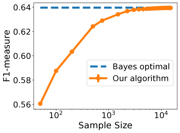
Figure 1: Convergence of our algorithm to Bayes optimal $F_{1}$ performance on synthetic multi-label data (see Section 7.1).

7.2 Real Data: Comparison with Other Algorithms

In the second set of experiments, we evaluated the performance of our algorithm on various benchmark multi-label data sets drawn from the Mulan repository. Details of the data sets are provided in Table 1. All the data sets come with prescribed train/test splits. After training our models on the training set, we measure the instance-averaged $F_{1}$ performance on the test set (i.e., we compute the multi-label $F_{1}$-measure on each test example and take the average).

We compared with the following algorithms: EFP (Dembczynski et al., 2013), LIMO (label-wise version recommended for instance-averaged $F_{1}$) (Wu & Zhou, 2017), and BR (which treats the $s$ labels as conditionally independent and trains $s$ binary logistic regression classifiers, one for each label). All algorithms were trained to learn linear models. Regularization parameters (for regularized logistic regression in our algorithm, EFP, and BR; and for the margin-based objective in LIMO) were chosen by 5-fold cross-validation on the training set from $\{10^{-4},\ldots,10^{3}\}$ (for all algorithms, the parameter value maximizing average $F_{1}$-measure across the 5 folds was selected). For our algorithm and EFP, as discussed in Section 6, we generally implemented the algorithms to estimate only a small subset of the $s^{2}+1$ statistics in ${\mathbf{q}}(x)$ (only those corresponding to numbers of active labels seen in the training data); for the Birds data set, this resulted in poor performance for both algorithms, and so for this data set we trained both algorithms to perform a full estimation of all $s^{2}+1$ statistics.

The results are shown in Table 2 (the asterisks in the results for the Birds data set denote the full estimation of $s^{2}+1$ statistics for this data set, as discussed above). As expected, the performance of our algorithm is similar to that of EFP. BR, as expected, is generally a relatively weak baseline. LIMO is sometimes competitive, but since it aims to simultaneously optimize several multi-label performance measures, we do not expect it to outperform algorithms designed for a specific performance measure, and indeed this is borne out in our experiments.

Table 1: Multi-label data sets used in experiments in Section 7.2.

Data set	# train	# test	# labels	# features
Scene	1211	1196	6	294
Yeast	1500	917	14	103
Birds	322	323	19	260
Medical	333	645	45	1449
Enron	1123	579	53	1001
Mediamill	30993	12914	101	120

Table 2: Comparison of $F_{1}$ performance of our algorithm with other MLC algorithms on various Mulan multi-label data sets. Higher values are better. See Section 7.2 for details and for an explanation of the asterisks for the Birds data set.

Data set	Our algorithm	EFP	LIMO	BR
Scene	0.7445	0.7426	0.6325	0.6009
Yeast	0.6571	0.6558	0.4914	0.6065
Birds	*0.5836	*0.5293	0.5463	0.5510
Medical	0.7557	0.7685	0.7237	0.6507
Enron	0.5868	0.6204	0.5764	0.5455
Mediamill	0.5642	0.5600	0.5135	0.5229

8 Conclusion

We have provided a family of convex calibrated surrogate losses for the multi-label $F_{\beta}$-measure, together with a quantitative regret transfer bound. Our surrogates effectively decompose the $F_{\beta}$ learning problem over $s$ labels into (at most) $s^{2}+1$ binary class probability estimation (CPE) problems. The regret transfer bound allows us to transfer any regret guarantees on the binary CPE learners to regret guarantees on the overall $F_{\beta}$ learner. Although motivated from a different viewpoint, like the EFP algorithm of Dembczynski et al. (2013), our algorithm can also be viewed as a type of ‘plug-in’ algorithm for the $F_{\beta}$-measure. While we have described the algorithm in the context of multi-label classification, the algorithm can also be used for binary sequence labeling tasks where the $F_{\beta}$-measure is useful.

Implementation of ‘decode’

In order to solve the combinatorial optimization problem involved in the mapping $\textup{{decode}}:{\mathbb{R}}^{s^{2}+1}{\rightarrow}\{0,1\}^{s}$ as defined in Eq. (LABEL:eqn:decode) efficiently, we make use of an $O(s^{3})$-time procedure due to Dembczynski et al. (2011). Specifically, Dembczynski et al. (2011) gave a procedure that, given a certain set of $s^{2}+1$ statistics of the true conditional distribution $p({\mathbf{y}}|x)$ at a point $x\in{\mathcal{X}}$, computes in $O(s^{3})$ time a Bayes optimal multi-label prediction $h^{*}(x)\in\{0,1\}^{s}$ at that point with respect to the $F_{1}$-measure by solving a similar combinatorial optimization problem (the approach generalizes easily to the $F_{\beta}$-measure for general $\beta$). Our algorithm (Algorithm 2) can be viewed as effectively estimating the same $s^{2}+1$ statistics from the training sample $S$; in particular, once a scoring function ${\mathbf{f}}_{S}:{\mathcal{X}}{\rightarrow}{\mathbb{R}}^{s^{2}+1}$ is learned by minimizing our surrogate loss $\psi$, the estimated statistics at a point $x\in{\mathcal{X}}$ are given by $\gamma^{-1}({\mathbf{f}}_{S}(x))$ (where $\gamma^{-1}$ is the inverse of the link function $\gamma:[0,1]{\rightarrow}{\mathbb{R}}$ associated with the strictly proper composite binary loss $\phi$ used in our surrogate, and is applied element-wise to ${\mathbf{f}}_{S}(x)$). Our ‘decode’ mapping effectively corresponds to estimating a Bayes optimal prediction at $x$ using these estimated statistics; we can therefore apply the procedure of Dembczynski et al. (2011) to these estimated statistics.

The implementation below is described for a general input vector ${\mathbf{u}}\in{\mathbb{R}}^{s^{2}+1}$ (see Eq. (LABEL:eqn:decode)); in our $F_{\beta}$ learning algorithm, to make a prediction at $x\in{\mathcal{X}}$, it would be applied to ${\mathbf{u}}={\mathbf{f}}_{S}(x)$. The overall idea is that the combinatorial search over $\widehat{{\mathbf{y}}}\in\{0,1\}^{s}$ is stratified over the $s+1$ sets $\widehat{{\mathcal{Y}}}_{l}=\{\widehat{{\mathbf{y}}}\in\{0,1\}^{s}:\|\widehat{{\mathbf{y}}}\|_{1}=l\}$, $l\in\{0,1,\ldots,s\}$; to find an optimal element $\widehat{{\mathbf{y}}}^{l,*}$ within each set $\widehat{{\mathcal{Y}}}_{l}$, one need only solve a problem of the form $\widehat{{\mathbf{y}}}^{l,*}\in\operatorname*{argmin}_{\widehat{{\mathbf{y}}}\in\widehat{{\mathcal{Y}}}_{l}}\sum_{j=1}^{s}\widehat{y}_{j}T_{jl}$ for certain numbers $T_{jl}$, which can be done simply by finding the smallest $l$ numbers among $\{T_{jl}:j\in[s]\}$ and setting the corresponding $l$ entries of $\widehat{{\mathbf{y}}}^{l,*}$ to 1 (and remaining entries to 0). Solving these $s+1$ subproblems and picking the best solution among them takes a total of $O(s^{2}\ln(s))$ time; computing the $s^{2}$ numbers $T_{jl}$ involves a matrix multiplication that takes a total of $O(s^{3})$ time.

Algorithm 2 Decode

1:  Input: Vector ${\mathbf{u}}=(u_{0},(u_{jk})_{j,k=1}^{s}))^{\top}\in{\mathbb{R}}^{s^{2}+1}$

2:  Parameters: Link function $\gamma:[0,1]{\rightarrow}{\mathbb{R}}$

3:  Define matrices ${\mathbf{Q}}\in[0,1]^{s\times s}$ and ${\mathbf{V}}\in{\mathbb{R}}^{s\times s}$ as follows:

$$Q_{jk} = \gamma^{-1}(u_{jk})$$

$$V_{kl} = \frac{-(1+\beta)^{2}}{\beta^{2}k+l}$$

4:  Compute ${\mathbf{T}}={\mathbf{Q}}{\mathbf{V}}$    // matrix multiplication, $O(s^{3})$ time

5:  For $l=1\ldots s$:                                 // for loop takes total $O(s^{2}\ln(s))$ time

6:    Find the $l$ smallest numbers among $\{T_{jl}:j\in[s]\}$; call the corresponding indices $j_{1}^{l},\ldots,j_{l}^{l}$

7:    Define $\widehat{{\mathbf{y}}}^{l,*}\in\{0,1\}^{s}$ as follows:

$$\widehat{y}^{l,*}_{j} = \left\{\begin{array}[]{ll}1&\text{if $j\in\{j_{1}^{l},\ldots,j_{l}^{l}\}$}\\ 0&\text{otherwise.}\end{array}\right.~{}~{}~{}{\color[rgb]{1,0,0}\text{// this solves $\widehat{{\mathbf{y}}}^{l,*}\in\textstyle{\operatorname*{argmin}_{\widehat{{\mathbf{y}}}\in\widehat{{\mathcal{Y}}}_{l}}\sum_{j=1}^{s}\widehat{y}_{j}T_{jl}}$}}$$

8:    Set $z^{*}_{l}=\sum_{j=1}^{s}\widehat{y}^{l,*}_{j}T_{jl}$

9:  End for

10:  Pick $\widehat{{\mathbf{y}}}^{*}\in\{0,1\}^{s}$ as follows:

$$\widehat{{\mathbf{y}}}^{*}\in\operatorname*{argmin}_{\widehat{{\mathbf{y}}}\in\{{\mathbf{0}},\,\widehat{{\mathbf{y}}}^{1,*},\ldots,\,\widehat{{\mathbf{y}}}^{s,*}\}}~{}-{\mathbf{1}}(\widehat{{\mathbf{y}}}={\mathbf{0}})\cdot\gamma^{-1}(u_{0})+{\mathbf{1}}(\widehat{{\mathbf{y}}}\neq{\mathbf{0}})\cdot z^{*}_{\|\widehat{{\mathbf{y}}}\|_{1}}$$

11:  Output: $\widehat{{\mathbf{y}}}^{*}\in\{0,1\}^{s}$

References

- Agarwal (2014) Agarwal, S. Surrogate regret bounds for bipartite ranking via strongly proper losses. Journal of Machine Learning Research, 15:1653–1674, 2014.
- Bartlett et al. (2006) Bartlett, P. L., Jordan, M., and McAuliffe, J. Convexity, classification and risk bounds. Journal of the American Statistical Association, 101(473):138–156, 2006.
- Dembczynski et al. (2010) Dembczynski, K., Cheng, W., and Hüllermeier, E. Bayes optimal multilabel classification via probabilistic classifier chains. In Proceedings of the 27th International Conference on Machine Learning (ICML), pp. 279–286, 2010.
- Dembczynski et al. (2011) Dembczynski, K., Waegeman, W., Cheng, W., and Hüllermeier, E. An exact algorithm for F-measure maximization. In Advances in Neural Information Processing Systems 24, pp. 1404–1412, 2011.
- Dembczynski et al. (2013) Dembczynski, K., Jachnik, A., Kotlowski, W., Waegeman, W., and Hüllermeier, E. Optimizing the F-measure in multi-label classification: Plug-in rule approach versus structured loss minimization. In Proceedings of the 30th International Conference on Machine Learning (ICML), pp. 1130–1138, 2013.
- Duchi et al. (2010) Duchi, J., Mackey, L., and Jordan, M. On the consistency of ranking algorithms. In Proceedings of the International Conference on Machine Learning (ICML), 2010.
- Gao & Zhou (2013) Gao, W. and Zhou, Z. On the consistency of multi-label learning. Artificial Intelligence, 199-200:22–44, 2013.
- Joachims (2005) Joachims, T. A support vector method for multivariate performance measures. In Raedt, L. D. and Wrobel, S. (eds.), Proceedings of the 22nd International Conference on Machine Learning (ICML), pp. 377–384, 2005.
- Koyejo et al. (2015) Koyejo, O., Natarajan, N., Ravikumar, P., and Dhillon, I. S. Consistent multilabel classification. In Advances in Neural Information Processing Systems 28, pp. 3321–3329, 2015.
- Parambath et al. (2014) Parambath, S. P., Usunier, N., and Grandvalet, Y. Optimizing F-measures by cost-sensitive classification. In Advances in Neural Information Processing Systems 27, pp. 2123–2131, 2014.
- Petterson & Caetano (2010) Petterson, J. and Caetano, T. S. Reverse multi-label learning. In Advances in Neural Information Processing Systems 23, pp. 1912–1920. 2010.
- Petterson & Caetano (2011) Petterson, J. and Caetano, T. S. Submodular multi-label learning. In Advances in Neural Information Processing Systems 24, pp. 1512–1520. 2011.
- Pillai et al. (2017) Pillai, I., Fumera, G., and Roli, F. Designing multi-label classifiers that maximize F measures: State of the art. Pattern Recognition, 61:394–404, 2017.
- Ramaswamy (2015) Ramaswamy, H. G. Design and Analysis of Consistent Algorithms for Multiclass Learning Problems. PhD thesis, Indian Institute of Science, 2015.
- Ramaswamy et al. (2013) Ramaswamy, H. G., Agarwal, S., and Tewari, A. Convex calibrated surrogates for low-rank loss matrices with applications to subset ranking losses. In Advances in Neural Information Processing Systems, 2013.
- Ramaswamy et al. (2014) Ramaswamy, H. G., Babu, B. S., Agarwal, S., and Williamson, R. C. On the consistency of output code based learning algorithms for multiclass learning problems. In Proceedings of the 27th Conference on Learning Theory (COLT), pp. 885–902, 2014.
- Ramaswamy et al. (2015) Ramaswamy, H. G., Tewari, A., and Agarwal, S. Convex calibrated surrogates for hierarchical classification. In Proceedings of the 32nd International Conference on Machine Learning (ICML), pp. 1852–1860, 2015.
- Reid & Williamson (2010) Reid, M. D. and Williamson, R. C. Composite binary losses. Journal of Machine Learning Research, 11:2387–2422, 2010.
- Steinwart (2007) Steinwart, I. How to compare different loss functions and their risks. Constructive Approximation, 26:225–287, 2007.
- Tewari & Bartlett (2007) Tewari, A. and Bartlett, P. L. On the consistency of multiclass classification methods. Journal of Machine Learning Research, 8:1007–1025, 2007.
- Tsochantiridis et al. (2005) Tsochantiridis, I., Joachims, T., Hoffman, T., and Altun, Y. Large margin methods for structured and interdependent output variables. Journal of Machine Learning Research, 6:1453–1484, 2005.
- Wu & Zhou (2017) Wu, X. and Zhou, Z. A unified view of multi-label performance measures. In Proceedings of the 34th International Conference on Machine Learning (ICML), pp. 3780–3788, 2017.
- Ye et al. (2012) Ye, N., Chai, K. M. A., Lee, W. S., and Chieu, H. L. Optimizing F-measure: A tale of two approaches. In Proceedings of the 29th International Conference on Machine Learning (ICML), 2012.
- Zhang & Zhou (2014) Zhang, M. and Zhou, Z. A review on multi-label learning algorithms. IEEE Transactions on Knowledge and Data Engineering, 26(8):1819–1837, 2014.
- Zhang (2004a) Zhang, T. Statistical behavior and consistency of classification methods based on convex risk minimization. Annals of Statistics, 32(1):56–134, 2004a.
- Zhang (2004b) Zhang, T. Statistical analysis of some multi-category large margin classification methods. Journal of Machine Learning Research, 5:1225–1251, 2004b.