On Symmetric Rectilinear Matrix Partitioning

Abstract

Even distribution of irregular workload to processing units is crucial for efficient parallelization in many applications. In this work, we are concerned with a spatial partitioning called rectilinear partitioning (also known as generalized block distribution) of sparse matrices. More specifically, in this work, we address the problem of symmetric rectilinear partitioning of a square matrix. By symmetric, we mean the rows and columns of the matrix are identically partitioned yielding a tiling where the diagonal tiles (blocks) will be squares. We first show that the optimal solution to this problem is NP-hard, and we propose four heuristics to solve two different variants of this problem. We present a thorough analysis of the computational complexities of those proposed heuristics. To make the proposed techniques more applicable in real life application scenarios, we further reduce their computational complexities by utilizing effective sparsification strategies together with an efficient sparse prefix-sum data structure. We experimentally show the proposed algorithms are efficient and effective on more than six hundred test matrices. With sparsification, our methods take less than $3$ seconds in the Twitter graph on a modern $24$ core system and output a solution whose load imbalance is no worse than $1\%$.

siscxxxxxxxx–x

05C70, 05C85, 68R10, 68W05

1 Introduction

After advances in social networks and the rise of web interactions, we are witnessing an enormous growth in the volume of generated data. A large portion of this data remains sparse and irregular and is stored as graphs or sparse matrices. However, analyzing data stored in those kinds of data structures is challenging, especially for traditional architectures due to the growing size and irregular data access pattern of these problems. High-performance processing of this data is an important and a pervasive research problem. There have been many studies developing parallel sparse matrix [11], linear-algebra [1, 3, 21, 2] and graph algorithms [29, 35, 38, 7, 16] for shared and distributed memory systems as well as GPUs and hybrid systems [15, 6, 22, 37]. In such platforms, the balanced distribution of the computation and data to the processors is crucial for achieving better efficiency.

In the literature, balanced partitioning techniques can be broadly divided into two categories: connectivity-based (e.g., [25, 8, 19, 9]) and spatial/geometric (e.g., [4, 30, 39, 33, 36]). Connectivity-based methods model the load balancing problem through a graph or a hypergraph. In general, computation volumes are weighted on the nodes and communication volumes are weighted on the edges or hyperedges. Connectivity-based techniques explicitly model the computation, and the communication, hence, they are generally computationally more expensive. This paper tackles the lightweight spatial (i.e., geometric) partitioning problem of two-dimensional sparse matrices, which mainly focuses on load-balancing, and communication is only implicitly minimized by localizing the data and neighbors that need the data.

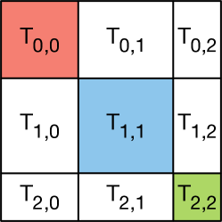
(a) An example partition

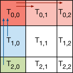
(b) Gather/Scatter data

Figure 1: Symmetric rectilinear matrix partitioning.

A large class of work uses two-dimensional sparse matrices in their design [20, 23, 5, 26]. For these applications, spatial partitioning methods focus on dividing the load using geometric properties of the workload. However, finding the optimal load distribution among the partitions and also minimizing the imposed communication (such as, the communication among neighboring parts) is a difficult problem. For instance, uniform partitioning is useful to regularize and limit the communication, but it ends up with highly imbalanced partitions. Some of the most commonly used spatial partitioning techniques like, Recursive Coordinate Bisection (RCB) [4], jagged (or $m$-way jagged) partitioning [39, 36] are useful to output balanced partitioning but may yield highly irregular communication patterns. Rectilinear partitioning (i.e., generalized block distribution) [30, 17] tries to address these issues by aligning two different partition vectors to rows and columns, respectively. In rectilinear partitioning, the tiles are arranged in an orthogonal, but unevenly spaced grid. This partitioning has three advantages; first, it limits the number of neighbors to 4 (or 8). Second, if communication along the logical rows and columns are needed, they will also be bounded to a smaller number of processors (e.g., for $P=p\times p$ processor system, it will be limited to $p$, i.e., $\sqrt{P}$). Third, more balanced blocks (in comparison to uniform partitioning) can be generated. Thus, the rectilinear partitioning gives a simple and well-structured communication pattern if the problem has a local communication structure.

In many applications where the internal data is square matrices, such as graph problems and iterative linear solvers for symmetric and non-symmetric square systems, the sparse matrix (the adjacency matrix in graph algorithms), represents the dependency of input elements to output elements. In many cases, the next iteration’s input elements are simply computed via linear operations on previous input’s output elements. For example, in graph algorithms, the inputs and outputs are simply the same entity, vertices of the graph. Hence, gathering information along the rows and then distributing the result along the columns is an essential step, and generic rectilinear partitioning would require additional communication for converting outputs of the previous iteration to inputs of next iteration. One natural way to address these issues is to use a conformal partitioning where diagonal tiles are squares. This is a restricted case of rectilinear partitioning in which a partition vector is aligned to rows and columns. We call this problem as Symmetric Rectilinear Partitioning Problem, which is also known as, the symmetric generalized block distribution [17].

This paper tackles the the Symmetric Rectilinear Partitioning Problem, finding an optimal rectilinear partitioning where diagonal tiles are squares (see Figure 1a). Here, we assume that the given matrix is square and we partition that matrix into $p\times p$ tiles such that by definition diagonal blocks will be squares. In this type of partitioning diagonal tiles are the owners of matching input and output elements. Hence, under this partitioning scheme distributing/gathering information along the rows/columns becomes very convenient (see Figure 1b). Also, in the context of graphs, each tile can be visualized as sub-graphs where diagonal tiles are the owners of the vertex meta-data and any other tile represents the edges between two sub-graphs. This type of partitioning becomes highly useful to reason about graph algorithms. For instance, in a concurrent work, we have leveraged the symmetric rectilinear partitioning for developing a block-based triangle counting formulation [40] that reduces data movement, during both sequential and parallel execution, and is also naturally suitable for heterogeneous architectures.

The optimal rectilinear partitioning problem was shown to be NP-hard by Grigni and Manne [17]. Symmetric rectilinear matrix partitioning is also a challenging problem even though it appeared to be simpler than the rectilinear matrix partitioning, yet until our work its complexity was unknown. In this work we show that the optimal symmetric rectilinear partitioning problem is also NP-hard. Here, we also define two variants of the symmetric rectilinear partitioning problem and we propose refinement-based and probe-based partitioning heuristics to solve these problems. Refinement-based heuristics [32, 30] apply a dimension reduction technique to map the two-dimensional problem into one dimension and compute a partition vector on one-dimensional data by running an optimal partitioning algorithm [32, 34]. Probe-based algorithms compute the partitioning vector by seeking for the best cut for each point. We combine lightweight spatial partitioning techniques with simple heuristics. Contributions of this work are as follows:

• Presenting two formulations for the symmetric rectilinear matrix partitioning problem; minLoadImbal (mLI), minNumCuts (mNC), which are dual problems of one another (Section 2).

• Proving that optimal symmetric rectilinear partitioning is NP-hard (Section 4).

• Proposing efficient and effective heuristics for the symmetric rectilinear partitioning problem (Section 5).

• Implementing an efficient sparse prefix-sum data structure to reduce the computational complexity of the algorithms (Section 6).

• Evaluating the effectiveness of sparsification techniques on the proposed algorithms (Section 7).

• Extensively evaluating the performance of proposed algorithms in different settings on more than six hundred real-world matrices (Section 9).

Our experimental results show that our proposed algorithms can very efficiently find good symmetric rectilinear partitions and output nearly the optimal solution on about $80$% of the $375$ small graphs and do not produce worse than $1.9$ times the optimal load imbalance. We have also run our algorithms on more than 600 matrices and hence experimentally validate the effectiveness of our proposed algorithms, as well as our proposed sparsification techniques and efficient sparse prefix-sum data structures. Our algorithms take less than $10$ seconds in the Twitter graph that has approximately $1.46$ billion edges on a modern $2\times 12$ core system. With sparsification, our algorithms can process Twitter graph in less than $3$ seconds and output a solution whose load imbalance is no worse than $1\%$.

2 Problem Definition and Notations

In this work, we are concerned with partitioning sparse matrices. Let $A$ be a two-dimensional square matrix of size $n\times n$ that has $m$ nonnegative nonzeros, representing the weights for spatial loads. In the context of this work, we are also interested in partitioning the adjacency matrix representation of graphs. A weighted directed graph $G=(V,E,w)$, consists of a set of vertices $V$, a set of edges $E$, and a function mapping edges to weights, $w:E\to\mathbb{R}^{+}$. A directed edge $e$ is referred to by $e=(u,v)\in E$, where $u,v\in V$, and $u$ is called the source of the edge, $v$ is called the destination. The neighbor list of a vertex $u\in V$ is defined as $N(u)=\{v\in V\mid(u,v)\in E\}$. We use $n$ and $m$ for the number of vertices and edges, respectively, i.e., $n=|V|$ and $m=|E|$. Let $A_{G}$ be the adjacency matrix representation of the graph $G$, that is, $A_{G}$ is an $n\times n$ matrix, where $\forall(u,v)\in E$, $A_{G}(u,v)=w(u,v)$, and everything else will be 0. Without loss of generality, we will assume source vertices are represented as rows, and destination vertices are represented as columns. In other words, elements of $N(u)$ will correspond to column indices of nonzero elements in row $u$. We will also simply refer to matrix $A_{G}$ as $A$ when $G$ is clear in the context. Table 1 lists the notation used in this paper.

Table 1: Notation used in this paper.

Symbol	Description
$G=(V,E,w)$	A weighted directed graph $G$ with a vertex set, $V$, a edge
	set, $E$, and a nonnegative real-value weight function $w$
$n=|V|$	number of vertices
$m=|E|$	number of edges
$A_{G}$	$n\times n$ adjacency matrix of $G$, or simplified as $A$
$A(i,j)$	the value at $i$th row and $j$th column in matrix $A$
$N(u)$	Neighbor list of vertex $u$
$\left[a\,..\,b\right]$	Integer interval, all integers between $a$ and $b$ included
$C$	A partition vector; $C=\left\langle c_{0},c_{1},\dots,c_{|C|-1}\right\rangle$, $c_{0}<\dots<c_{|C|-1}$
$C(i)$	The $i$th lowest element in partition vector $C$, i.e., $c_{i}$.
$C_{r}$, $C_{c}$	Row and column partition vectors
$T_{i,j}$	Tile $i,j$
$\phi(T_{i,j})$	Load of $T_{i,j}$, i.e., sum of the nonzeros in $T_{i,j}$
$L_{max}(A,C_{r},C_{c})$	Maximum load among all tiles
$L_{avg}(A,C_{r},C_{c})$	Average load of all tiles
$\lambda(A,C_{r},C_{c})$	Load imbalance for partition vectors, or simplified as $\lambda$
$\lambda(A,C_{r},C_{c},k)$	Load imbalance among $T_{i,j}$ st. $i,j\leq k$
$s$	Sparsification factor where $s\in[0,1]$
$\epsilon$	Error tolerance for automatic sparsification factor selection

Given an integer $p$, $1\leq p\leq n$, let $C=\left\langle c_{0},c_{1},\dots,c_{p}\right\rangle$ be a partition vector that consists of sequence of $p+1$ integers such that $0=c_{0}<c_{1}<\dots<c_{p}=n$. Then $C$ defines a partition of $\left[0\,..\,n-1\right]$ into $p$ integer intervals $\left[c_{i}\,..\,c_{i+1}-1\right]$ for $0\leq i\leq p-1$.

Definition 2.1.

Rectilinear Partitioning. Given $A$, and two integers, $p$ and $q$, a rectilinear partitioning consists of a partition of $\left[0\,..\,n-1\right]$ into $p$ intervals ($C_{r}$, for rows) and into $q$ intervals ($C_{c}$, for columns) such that $A$ is partitioned into non-overlapping $p\times q$ contiguous tiles.

In rectilinear partitioning, a row partition vector, $C_{r}$, and a column partition vector, $C_{c}$, together generate $p\times q$ tiles. For $i\in[0..p-1]$ and $j\in[0..q-1]$, we denote $(i,j)$-th tile by $T_{i,j}$. $\phi(T_{i,j})$ denotes the load of $T_{i,j}$, i.e., the sum of nonzero values in $T_{i,j}$. Given partition vectors, quality of partitioning can be defined using load imbalance, $\lambda$, among the tiles, which is computed as

$$\lambda(A,C_{r},C_{c})=\frac{L_{max}(A,C_{r},C_{c})}{L_{avg}(A,C_{r},C_{c})}$$

where

$$L_{max}(A,C_{r},C_{c})=\max_{i,j}\phi(T_{i,j})$$

and

$$L_{avg}(A,C_{r},C_{c})=\frac{\sum_{i,j}\phi(T_{i,j})}{p\times q}.$$

A solution which is perfectly balanced achieves a load imbalance, $\lambda$, of $1$. Figure 2a presents a toy example for rectilinear partitioning where $C_{r}=\left\langle 0,1,4,6\right\rangle$, $C_{c}=\left\langle 0,3,5,6\right\rangle$ and $\lambda(A,C_{r},C_{c})=\frac{3}{(14/9)}\approx 1.9$ when we assume that all nonzeros are equal to $1$.

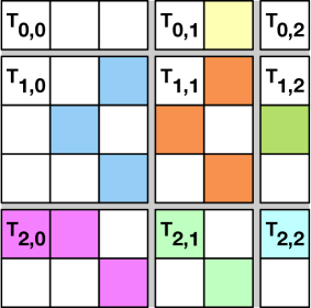
(a) Non-Symmetric: $C_{r}=\{0,1,4,6\}$, $C_{c}=\{0,3,5,6\}$

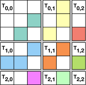
(b) Symmetric: $C=\{0,3,5,6\}$

Figure 2: $3\times 3$ Non-Symmetric/Symmetric rectilinear partitioning examples on the adjacency matrix representation of the toy graph in Figure 4a.

Definition 2.2.

Symmetric Rectilinear Partitioning. Given $A$ and $p$, symmetric rectilinear partitioning can be defined as partitioning $\left[0\,..\,n-1\right]$ into $p$ intervals, applying which to both rows and columns, such that $A$ partitions into $p\times p$ non-overlapping contiguous tiles where diagonal tiles are squares.

In symmetric rectilinear partitioning, the same partition vector, $C_{c}=C=C_{r}$, is used for row and column partitioning. Figure 2b presents a toy example for the symmetric rectilinear partitioning where $C=\left\langle 0,3,5,6\right\rangle$ and $\lambda(A,C,C)=\frac{3}{(14/9)}\approx 1.9$.

In the context of this work, we consider two symmetric rectilinear partitioning problems; minLoadImbal and minNumCuts. These two problems are the dual of each other.

Definition 2.3.

minLoadImbal (mLI ​) Problem. Given a matrix $A$ and an integer $p$, the mLI problem consists in finding the optimal partition vector, $C$, of size $p$ that minimizes the load imbalance:

$$\text{\sc mLI}(A,p) =\min_{C}\lambda(A,C,C)$$

Definition 2.4.

minNumCuts (mNC ​) Problem. Given a matrix $A$ and a maximum load limit $Z$, the mNC problem consists of finding the minimum number of intervals $p$ that will partition the matrix $A$ so that the sum of nonzeros in all tiles are bounded by $Z$.

$$\text{\sc mNC}(A,Z)=\min_{C}|C|,$$

$$\text{ s.t. }L_{max}(A,C,C)\leq Z$$

3 Related Work

Two-dimensional matrix distributions have been widely used in dense linear algebra [20, 28]. Cartesian [20] distributions (see Figure 3a) where the same partitioning vector is used to partition rows and columns are widely used. This is due to the partitioned matrix naturally mapping onto a two-dimensional mesh of processors. This kind of partitioning becomes highly useful to limit the total number of messages on distributed settings. Dense matrices or well structured sparse matrices can be easily partitioned with cartesian partitioning. However, for sparse and irregular problems finding a good vector that can be aligned with both dimensions is a hard problem. Therefore, many non-cartesian two-dimensional matrix partitioning methods have been proposed [4, 31, 32, 30, 39, 36] for sparse and irregular problems. As a class of shapes, rectangles implicitly minimize communication, allow many potential allocations, and can be implemented efficiently with simple operations and data structures. For these reasons, they are the main preferred shape. For instance, recursive coordinate bisection (RCB) [4] is a widely used technique that rely on a recursive decomposition of the domain (see Figure 3c). Another widely used technique is called jagged partitioning [39, 36] which can be simply achieved by first partitioning the matrix into one-dimensional (1D) row-wise or column-wise partitioning, then independently partitioning in each part (see Figure 3d).

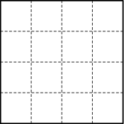
(a) Cartesian

(b) Rectilinear

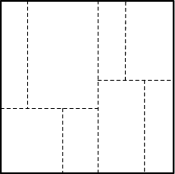
(c) RCB

(d) Jagged

Figure 3: Spatial partitioning examples.

One way to overcome the hardness of proposing one partition vector for rows and columns is to propose different partition vectors for rows and columns. This problem is named as rectilinear partitioning [32] (or generalized block distribution [30]). Independently, Nicol [32] and Manne and Sørevik [30] proposed an algorithm to solve this problem that is based on iteratively improving a given solution by alternating between row and column partitioning. These algorithms transform two-dimensional (2D) rectilinear partitioning problem into 1D partitioning problem using a heuristic and iteratively improves the solution, in which the load of a interval is calculated as the maximum of loads in columns/rows in the interval of rows/columns. This refinement technique is presented in Algorithm 1. Here, optimal1DPartition($P$) [32] is a function that returns the optimal partition on rows of $P$. Hence, Algorithm 1 returns the optimal 1D row partition for the given column partition $C_{c}$.

 $\triangleright$ $P$ is a $n\times p$ matrix to store interval sums for each row

1 $P(i,j)\leftarrow 0$, for $i\in\left[0\,..\,n\right]$ and $j\in\left[0\,..\,p-1\right]$

2

 $\triangleright$ for each row

3 for $i=0$ to $n-1$ do

4       for each $j$, where $A(i,j)\neq 0$ do

             $k\leftarrow 0$

             $\triangleright$ Interval index

5             while $j\geq C_{c}(k+1)$ do

                   $k\leftarrow k+1$

                   $\triangleright$ Find the interval

6                  

7            $P(i+1,k)\leftarrow P(i+1,k)+A(i+1,j)$

8            

9      

10

 $\triangleright$ Compute $p$ prefix sums for each interval

11 for $j=0$ to $p-1$ do

12       for $i=1$ to $n$ do

13             $P(i,j)\leftarrow P(i,j)+P(i-1,j)$

14            

15      

16

 $\triangleright$ Return the optimal partitioning on rows of $P$

17 return optimal1DPartition($P$)

Algorithm 1 refinement($A,C_{c},p$)

The optimal solution of the rectilinear partitioning was shown to be NP-hard by Grigni and Manne [17]. In fact, their proof shows that the problem is NP-hard to approximate within any factor less than $2$. Khanna et al. [27] have shown the problem to be constant-factor approximable.

Rectilinear partitioning may still cause high load-imbalance due to generalization. Jagged partitions [39] (also called Semi Generalized Block Distribution [17]) tries to overcome this problem by distinguishing between the main dimension and the auxiliary dimension (see Figure 3d). The main dimension is split into $p$ intervals and each of these intervals partition into $q$ rectangles in the auxiliary dimension. Each rectangle of the solution must have its main dimension matching one of these intervals. The auxiliary dimension of each rectangle is arbitrary. We refer readers to Saule et al. [36] which presents multiple variants and generalization of jagged partitioning, and also detailed comparisons of various 2D partitioning techniques.

Most of the algorithms we present require querying the load in a rectangular tile and this problem is known as the dominance counting problem in the literature [24]. Given a set of $d$-dimensional points $S$ and a $d$-dimensional query point $x=\left\langle x_{1},\ldots,x_{d}\right\rangle$, dominance counting problem returns the number of points $y=\left\langle y_{1},\ldots,y_{d}\right\rangle$, such that $y\in S$, and $y_{i}\leq x_{i},\forall i\in\left[1\,..\,d\right]$. [24] presents an efficient data structure that can answer such queries in $O\left(\frac{\log|S|}{\log\log|S|}\right)$ time with $O(|S|)$ space usage. However, this data structure is very complex and hard to implement. Hence we propose another data structure that we are going to cover in Section 6.

4 Symmetric Rectilinear Partitioning is NP-hard

We first define the decision problem of the symmetric rectilinear partitioning for the proof.

Definition 4.1.

Decision Problem of the Symmetric Rectilinear Partitioning. Given a matrix $A$, the number of intervals $p$, and a value $Z$, decision problem of the symmetric rectilinear partitioning (SRP) seeks whether there is a partition vector of size $p+1$ such that the sum of the nonzero values in each tiles are bounded by $Z$.

It’s clear SRP is in NP. We show that it is NP-complete by reducing a well-known NP-complete problem, vertex cover problem(VC), to SRP.

Definition 4.2.

Vertex Cover Problem (VC). Given an undirected graph $G=(V,E)$ and an integer $K$, VC is to decide whether there exist a subset $V^{\prime}$ of the vertices of size $K$ such that at least one end point of every edge is in $V^{\prime}$, i.e., $\forall(u,v)\in E$, either $u\in V^{\prime}$ or $v\in V^{\prime}$.

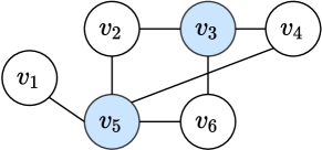
(a) Graph

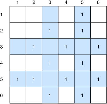
(b) Adjacency matrix

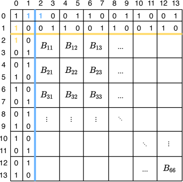
(c) Transformation

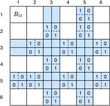
(d) Tile matrix

Figure 4: A toy example for VC $(K=2)$ and its equivalent SRP instance $(Z=1,p=10)$

Figure 4a illustrates a toy example for VC. In this example the graph consists of $6$ vertices and $7$ edges. For $K=2$, $V^{\prime}=\{v_{3},v_{5}\}$ is a solution.

We extend Grigni and Manne’s [17] input reduction technique to reduce VC to SRP. Given a graph $G=(V,E)$, $V=\{v_{1},v_{2},\dots,v_{n}\}$, its adjacency matrix $A$ (see Figure 4b), and an integer $K$ we apply six transformation steps. First, we create a new square binary matrix, $A^{\prime}$, of size $(2n+2)\times(2n+2)$, initialized with zeros (see Figure 4c). Second, we limit the sum of nonzeros in each result tile to be at most one ($Z=1$). This limitation allows us to enforce cuts by placing nonzeros at adjacent positions in the matrix. For instance, in Figure 4c, consequent nonzeros at $A^{\prime}(0,1)$ and $A^{\prime}(0,2)$ enforce a cut between the column $1$ and the column $2$. Two sample cuts are highlighted in Figure 4c. As the third step, we initialize the first two rows and two columns as follows: we set $A^{\prime}(0,0)=1$, then in first row and column we put two $1$s followed by two $0$s, until the end of row or column. Similarly, starting $A^{\prime}(1,1)$ position in second row and column, we now first put two $0$s followed by two $1$s. Fourth, the rest of the $A^{\prime}$ matrix is tiled as $n\times n$ tiles of sizes $2\times 2$ (see Figure 4c). Here, let $B_{i,j}$ represent the $2\times 2$ tile located at position $A^{\prime}(2i,2j)$ in the matrix, where $i,j\in\left[1\,..\,n\right]$. Fifth, we initialize each $B_{i,j}$ with an identity matrix of size two ($I_{2}$) if $A(i,j)=1$ (see Figure 4d). Since we limit the number of nonzero elements in each result tile to be at most one, an identity matrix has to be cut by at least one horizontal or vertical cut. Last, we set the number of intervals, $p$, as $n+2+K$, thus, $n+3+K$ cuts will be sought. With the enforced $n+1$ cuts from the third step and the $2$ cuts at the beginning and the end, possible cuts left are only in between of each row (and column) of the $2\times 2$ tiles and there are only $n$ of them. Thus the problem becomes, choosing $K$ rows (columns) of $2\times 2$ tiles to be cut, among $n$ possible cuts, s.t., all $2\times 2$ identity matrices are covered.

The equivalence between the constructed SRP instance and the VC comes from both about choosing rows and columns to cover the nonzero elements. They only differ in choosing elements, the former is a $2\times 2$ matrix, and the latter is $1\times 1$ matrix, as shown with the example in Figure 4d and Figure 4b. The formal proof shows there is a solution for one instance if and only if there is for the other, as follows.

Proof 4.3.

NP-Completeness Proof of SRP. Let $C$ denote the partition vector. Let a set $S_{0}$ contains the trivial cuts in $C$, i.e., $\left\langle 0,2n+2\right\rangle$, set $S_{1}$ contains the forced cuts, i.e., $\{1\}\cup\{2i\mid i\in[1,n]\}$, and $S_{2}$ contains the remainder cuts in $C$.

$\Rightarrow$ Suppose $V^{\prime}$ is a solution to the VC instance. Then, let $S_{2}=\{2i+1|v_{i}\in V^{\prime}\}$. Since $|S_{0}\cup S_{1}|=3+n$, and $|S_{2}|=K$, we have $|C|=n+3+K=p+1$.

The tiles in first two rows and columns all have a load of at most 1 after the forced cuts. For the rest of the $2\times 2$ nonzero tiles $B_{i,j}$, we have the following:

$$B_{i,j}\text{ is an identity matrix} \implies A(i,j)\neq 0$$

$$\implies v_{i}\in V^{\prime}\text{~{}or~{}}v_{j}\in V^{\prime}$$

$$\implies 2i+1\in S_{2}\text{~{}or~{}}2j+1\in S_{2}$$

All nonzero $B_{i,j}$ are cut by $S_{2}$ such that the load is at most 1 for tiles, showing $C$ is valid.

$\Leftarrow$ a similar logic can be applied in the reverse order to complete the proof. We are omitting for the sake of brevity.

4.1 A mathematical model for the SRP problem

To the best of our knowledge, this is the first work that tackles the symmetric rectilinear partitioning problem. Symmetric rectilinear partitioning is a restricted problem, therefore comparing our algorithms with more relaxed partitioning algorithms (such as jagged, rectilinear etc.) does not provide enough information about the quality of the found partition vectors. Hence, we implemented a mathematical model that finds the optimal solution and run this model on small matrices to compare optimal solutions with the output of our algorithms.

minimize $$\quad{L_{\text{max}}}$$

subject to

(1) $$C =\left\langle 0=c_{0}<c_{1}\dots c_{p-1}<c_{p}=n\right\rangle$$

(2) $$I(i,j) =1\iff c_{i}\leq j \scriptstyle(i=0,\dots,p)(j=0,\dots,n-1)$$

(3) $$X(i,j,u,v) =1\iff 2=I(c_{i},u)-I(c_{i+1},u) \scriptstyle(i,j=0,1,\dots,p-1)$$

$$\qquad\qquad+I(c_{j},v)-I(c_{j+1},v) \scriptstyle(u,v=0,\dots,n-1)$$

(4) $$\phi(i,j) =\sum_{u,v=0,\dots,n-1}X(i,j,u,v)\times A(u,v) \scriptstyle(i,j=0,1,\dots,p-1)$$

(5) $$L_{\text{max}} \geq\phi(i,j) \scriptstyle(i,j=0,1,\dots,p-1)$$

In the above model, the $C$ vector (Equation 1) represents the monotonic cut vector where each cut is an integer; $C\in\mathbb{Z}^{(p+1)}$. $I$ denotes a $(p+1)\times n$ binary matrix, i.e., $I\in\{0,1\}^{(p+1)\times n}$, where $I(i,j)=1$ if and only if the $i^{th}$ cut is to the left of $j^{th}$ column. The $I$ matrix allows us to identify in which partition a row/column appears, for example $I(c_{i},j)-I(c_{i+1},j)=1$ if and only if $j$th row/column is in the $i$th partition. $X$ is a binary $p\times p\times n\times n$ matrix. $X(i,j,u,v)=1$ if and only if $A(u,v)$ is in tile $T_{i,j}$. As shown in Equation 3 $X$ can be constructed using $I$. Then, using $X$, we can represent tile loads as presented in Equation 4. Finally, we define a variable, $L_{\text{max}}$ that stores the load of a maximum loaded tile and the goal of the above model is to minimize $L_{\text{max}}$.

5 Algorithms for Symmetric Rectilinear Partitioning

We propose two algorithms for the mLI problem (Definition. 2.3) and two algorithms for the mNC problem (Definition. 2.4). At a high level, those algorithms can be classified as refinement-based and probe-based. In this section, we explain how these algorithms are designed.

5.1 minLoadImbal (mLI) problem

We propose two algorithms for the mLI problem. One of those algorithms, Refine a cut (RaC) adopts previously defined refinement technique (see Algorithm 1) into the symmetric rectilinear partitioning problem. Note that the RaC algorithm has no convergence guarantee. The second algorithm, Bound a cut (Bull. astr. Inst. Czechosl.), implements a generic algorithm that takes an algorithm which solves the mNC problem as input and solves the mLI problem.

5.1.1 Refine a cut (RaC)

RaC algorithm first applies the refinement on rows, and then on columns independently. Then it computes the load imbalances for the generated partition vectors. The RaC algorithm chooses the direction (row or column) that gives a better load imbalance. Then, iteratively applies the refinement algorithm only in this direction until it reaches the iteration limit ($\tau$). This procedure is presented in the Algorithm 2.

 $\triangleright$ Current ($C$) and previous ($C^{\prime}$) partition vectors

1 $C(0)\leftarrow 0$; $C(j)\leftarrow n$, for $1\leq j\leq p$

2

 $\triangleright$ Apply 1D partitioning refinement

$C_{r}\leftarrow$ refinement($A,C,p$)

  $\triangleright$ Row based

$C_{c}\leftarrow$ refinement($A^{T},C,p$)

  $\triangleright$ Column based

3

 $\triangleright$ Aligning same partition vector for rows and columns

$L_{r}\leftarrow\lambda(A,C_{r},C_{r})$

  $\triangleright$ Row based imbalance

$L_{c}\leftarrow\lambda(A,C_{c},C_{c})$

  $\triangleright$ Column based imbalance

4 if  $L_{r}<L_{c}$  then

5       $C\leftarrow C_{r}$

6      

7else

8       $C\leftarrow C_{c}$

9       $A\leftarrow A^{T}$

10      

11

12$i\leftarrow 0$

13 while  $i<\tau$  do

14       $C\leftarrow$ refinement($A,C,p$)

15       $i\leftarrow i+1$

16      

17

return $C$

Algorithm 2 RaC($A,p$)

The primary advantage of this algorithm is its simplicity. This algorithm can be easily parallelized as shown in [30, 32]. However, choosing a direction at the beginning may result in a missed opportunity to converge to a better partition vector using the other direction.

5.1.2 Bound a cut (Bull. astr. Inst. Czechosl.)

Bull. astr. Inst. Czechosl.algorithm solves the mLI problem given an algorithm that solves the mNC problem. Given a matrix $A$ and an integer $p$, the Bull. astr. Inst. Czechosl.algorithm seeks for the minimal load size, $B$, such that mNC algorithm returns a partition vector of size $p+1$. In this approach, the Bull. astr. Inst. Czechosl.algorithm does a binary search over the range starting from $0$ to the sum of nonzeros. In each iteration of the binary search, it runs mNC algorithm with the middle target load between lower and upper bounds, and halves the search space. This procedure is presented in the Algorithm 3. Note that binary searching on the exponent first and then on the fraction can enable efficient float value binary search in order to deal with the machine precision of real values.

 $\triangleright$ Initialize temporary partition vector

1 $C(0)\leftarrow 0$; $C(j)\leftarrow n$, for $1\leq j\leq p+1$

2

3$l\leftarrow 0$

4 $r\leftarrow\sum_{0\leq u,v<n}A(u,v)$

5

 $\triangleright$ Probe in binary search fashion

6 while $l<r$ do

7       $B\leftarrow(l+r)/2$

8       $C\leftarrow$ mNC ($A,B$)

9       if $|C|\leq p+1$ then

10             $r\leftarrow B$

11            

12      else

13             $l\leftarrow B+1$

14            

15      

16

return mNC ($A,l$)

Algorithm 3 Bull. astr. Inst. Czechosl.($A,p$)

5.2 minNumCuts (mNC) problem

Given a matrix, $A$, and an integer, $Z$, the mNC problem aims to output a partition vector, $C$, with the minimum number of intervals, $p$, where the maximum load of a tile in the corresponding partitioning is less than $Z$, i.e., $\max_{0\leq i,j\leq p}\phi(T_{i,j})\leq Z$.

1

 $\triangleright$ Initially we do not know partition vector’s size

2 $C(0)\leftarrow 0$

3 $i\leftarrow 1$

4 while $C(i-1)\neq n$ do

5       $C(i)\leftarrow\beta(A,C,i,Z)$

6       $i\leftarrow i+1$

7      

8

9return $C$

Algorithm 4 PaL($A,Z$)

5.2.1 Probe a load (PaL)

Compared to our refinement based algorithm (RaC) which does not have any convergence guarantee, the PaL algorithm guarantees outputting a partition vector at the local optimal in the sense that removal or moving forward of any of the cuts will increase the maximum load. That’s why the PaL algorithm is more stable and usually performs better than the RaC algorithm. PaL is illustrated in Algorithm 4. The elements of $C$ are found through binary search, $\beta$, on the matrix. In this algorithm, $\beta(A,C,i,Z)$, searches $A$ in the $\left[C[i-1]\,..\,n\right]$ to compute the largest $i^{th}$ cut point such that $\max_{0\leq j,k\leq t}\{\phi(T_{j,k})\}\leq Z$. Note that the PaL algorithm considers more cases in a two-dimensional fashion.

5.2.2 Ordered probe a load (oPaL)

The oPaL algorithm tries to reduce computational complexity of the PaL algorithm by applying a coordinate transformation technique to the input matrix, presented in Algorithm 5. In Algorithm 5, $A^{\prime}$ is a three-dimensional matrix where $A^{\prime}(\max(i,j),\min(i,j),i>j)=v$, if $A(i,j)=v$. To construct $A^{\prime}$, for each nonzero, $A(i,j)\neq 0$, in the $A$ matrix, if $i>j$, we assign $A^{\prime}(i,j,$ True$)=v$, and otherwise $A^{\prime}(i,j,$ False$)=v$. Note that, we visit each nonzero in $A$ following the row-major order and update $A^{\prime}$ accordingly. To avoid dynamic or dense memory allocations, we first, pre-calculate size of each row, i.e., $A^{\prime}(i,:,:)$, then allocate and insert nonzeros.

1

 $\triangleright$ Initialize the three-dimensional matrix

2 $A^{\prime}(i,j,b)\leftarrow 0$, for $0\leq i,j\leq n-1$ and $b\in$ {True, False}

3

4for each $i=0$ to $n-1$ do

5       for each $j=0$ to $n-1$ do

6             if $A(i,j)\neq 0$ then

7                   $A^{\prime}(\max(i,j),\min(i,j),i>j)\leftarrow A(i,j)$

8                  

9            

10      

11

12return $A^{\prime}$

Algorithm 5 Transform($A$)

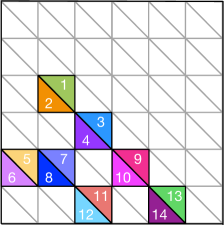
(a) Transformed matrix, $A^{\prime}$

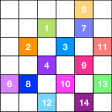
(b) Order of nonzeros

Figure 5: An example transformation for the toy graph in Figure 4a. Figure 5a $A^{\prime}(\max(i,j),\min(i,j),i>j)=A(i,j)$. In Figure 5a, upper triangles represent $(i\leq j)$ and lower triangles represent $(i>j)$ for the third dimension in each cell. Figure 5b illustrates the adjacency matrix where the order of each nonzero written in the corresponding cell when $A^{\prime}$ is accessed in row-major order.

After the transformation, going over the transformed matrix in row-major order becomes equivalent to going over the original matrix in the diagonal-major order (see Figure 5b). Hence, we can make a single pass over the whole matrix to compute the same partition vector as the PaL algorithm.

oPaL is presented in Algorithm 6. When we are going over the transformed matrix in row-major order, we are trying to find the furthest point from the previous cut so that if we put the next cut at that point, none of the newly created tiles will exceed the load bound $Z$. When processing a single nonzero, we first find which of the newly created tiles it will fall into and increment its load by the weight of the nonzero. Then we update the maximum load of the newly created tiles, $l_{\text{max}}$. We stop when $l_{\text{max}}$ exceeds $Z$ and add the index of the row we are currently processing to the partition vector $C$. The algorithm terminates either when all the nonzeros have been processed or when two of the same cuts are present in $C$ indicating infeasibility of partitioning with a load bound of $Z$. Note that the PaL and the oPaL algorithms outputs the same partition vector. Our goal to propose the oPaL algorithm is to decrease the computational complexity of the PaL algorithm. The PaL algorithm is pleasingly parallel, hence the execution time can be decreased significantly on a multi-core machine. However, on sequential execution the PaL algorithm’s complexity is worse than the oPaL algorithm. Hence, the oPaL algorithm is highly beneficial for the sequential execution and the PaL algorithm is better to use on parallel settings.

1

2$A^{\prime}\leftarrow$ Transform($A$)

$C(0)\leftarrow 0$

  $\triangleright$ Initially we do not know partition vector’s size

$c\leftarrow 1$

  $\triangleright$ Track cut indices

3 $i\leftarrow 0$

4 while $i<n$ do

       $L_{1}(c)\leftarrow 0$, for $0\leq c\leq|C|-1$

        $\triangleright$ Lower triangle and diagonal loads

       $L_{2}(c)\leftarrow 0$, for $0\leq c\leq|C|-1$

        $\triangleright$ Upper triangle loads

5       $l_{\text{max}}\leftarrow 0$

6       while $i<n$ do $\triangleright$ To find the next cut

7             for each $j=0$ to $n-1$ and $b\in\{$ True, False $\}$ do

8                   if $A^{\prime}(i,j,b)\neq 0$  then

9                         $v\leftarrow A^{\prime}(i,j,b)$

10                         $t\leftarrow\max_{t}\{t\mid C(t)\leq j\}$

11                         if  $b=$True or $t=|C|-1$ then $\triangleright$ A lower or a diagonal tile

12                               $L_{1}(t)\leftarrow L_{1}(t)+v$

13                               $l_{\text{max}}\leftarrow\max(l_{\text{max}},L_{1}(t))$

14                              

15                        else

16                               $L_{2}(t)\leftarrow L_{2}(t)+v$

17                               $l_{\text{max}}\leftarrow\max(l_{\text{max}},L_{2}(t))$

18                              

19                        if $l_{\text{max}}>Z$ then

20                               break

21                              

22                        

23                  

24            if $l_{\text{max}}>Z$ then

25                   break

26                  

27            $i\leftarrow i+1$

28            

29      if $C(c-1)=i$ then

             break

              $\triangleright$ Infeasible $Z$

30            

31      

      $C(c)\leftarrow i$

        $\triangleright$ Append new cut to the partition vector

       $c\leftarrow c+1$

        $\triangleright$ Increment index

32      

33

34return $C$

Algorithm 6 oPaL($A,Z$)

5.2.3 Bound a load (BaL)

One can solve the mNC problem using any algorithm that is proposed for solving the mLI problem, using binary searches over the possible number of cuts. We call this procedure as bounding a load (BaL), displayed in Algorithm 7. This approach can be improved in certain cases by bounding the search space of the candidate number of cuts to decrease the number of iterations. For instance, when the given matrix is binary, the search space can be initialized as $[1,\lceil\frac{n}{\lceil\sqrt{Z}\rceil}\rceil]$, where the upper bound is derived by considering the dimension $\lceil\sqrt{Z}\rceil$ of the smallest matrix that can contain $Z$ nonzeros.

1

 $\triangleright$ $l$ and $u$ are the upper and lower bounds

$l\leftarrow 1$

 $\triangleright$ At least 1 cut

$u\leftarrow n$

 $\triangleright$ Number of rows

2

3while $l<u$ do

4       $p\leftarrow(l+u)/2$

5       $C\leftarrow$ mLI ($A,p$)

6       $Z^{\prime}\leftarrow L_{max}(A,C,C)$

7       if $Z^{\prime}<Z$ then

8             $u\leftarrow p$

9            

10      else

11             $l\leftarrow p+1$

12            

13      

14

return mLI ($A,l$)

Algorithm 7 BaL($A,Z$)

6 Sparse Prefix Sum data structure and Computational Complexity

Given the partition vectors, querying numbers of nonzeros in each tile is one of the computationally heavy steps of our proposed algorithms; a naive approach requires iterating over all edges. We address this issue by proposing a data structure to reduce the complexity of this query and thus reduce the complexity of our algorithms.

 $\triangleright$ Assuming that 1-based indexing is used for matrix $A$ and $A\geq 0$

1

 $\triangleright$ Initialize a zero $n\times n$ sparse matrix

2 $S(i,j)\leftarrow 0$ for $1\leq i,j\leq n$

3

4for each $i=1$ to $n$ do

5       for each $j=1$ to $n$ do

6             if $A(i,j)\neq 0$ then

7                   $v\leftarrow A(i,j)$

8                   $t\leftarrow j$

9                   while $t\leq n$ do

10                         $S(i,t)\leftarrow v+\max_{k\leq i}S(k,t)$

                        

                         $\triangleright$ Increment $t$ by adding its least significant bit to itself.

11                         $t\leftarrow t+$ LSB$(t)$

12                        

13                  

14            

15      

16

return $S$

Algorithm 8 SPSConstruction($A$)

6.1 Sparse prefix sum data structure

One can query number nonzeros within a rectangle using a two-dimensional cumulative sum matrix in constant time. However, such a matrix requires $\Theta(n^{2})$ space, which is infeasible for large problem instances. Here, we propose an elastic sparse prefix sum data structure which can query the load of a rectangle in $O(\log^{2}n)$ time and requires $O(m\log n)$ memory space. The data structure is essentially a persistent Binary Indexed Tree (BIT) [14]. We use fat node approach to transform BIT into a persistent data structure as described in [13]. BIT is a data structure to query and maintain prefix sums in a one-dimensional array of length $n$ using $O(n)$ space and $O(\log n)$ time. Persistent data structures are dynamic data structures that let you query from a previous version of it. The column indices of the nonzeros are inserted into the BIT in a row major order with version number being the row index of the nonzeros. Algorithm 8 presents the high-level algorithm and Figure 6 illustrates an example representation of our data structure for the toy graph presented in Figure 4a. In Figure 6 tree on the left is used to construct the data structure (see line 8 in Algorithm 8). For instance, based on that example $A(i=1,j=5)\neq 0$, hence $i=1$ is the version number and we update $5^{\text{th}}$ and $6^{\text{th}}$ indices (see tree for insertions in Figure 6) of the first version. Also, $A(i=2,j=5)\neq 0$ hence $i=2$ is the version number and again we need to update $5^{\text{th}}$ and $6^{\text{th}}$ indices of the second version. Since we use the fat node approach to provide persistence; in the second version we fetch the values of $5^{\text{th}}$ and $6^{\text{th}}$ indices from the closest previous version and then update the second version (see line 8 in Algorithm 8) by setting the values of those indices as $2$.

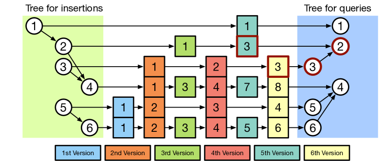
Figure 6: An illustration of our sparse prefix sum data structure on the toy graph presented in Figure 4a. Sum of the highlighted cells gives us the result a query for the $3^{rd}$ index from version $6$ which is the load of the rectangle from $(1,1)$ to $(6,3)$ that is equal to 6.

 $\triangleright$ Assuming that $i,j$ are 1-based indices and $S\leftarrow$ SPSConstruction(A)

1 $r\leftarrow 0$

2 while $j>0$ do

3       $r\leftarrow r+\max_{k\leq i}S(k,j)$

      

       $\triangleright$ Decrement $j$ by clearing its least significant bit.

4       $j\leftarrow j-$ LSB$(j)$

5      

6

7return $r$

Algorithm 9 SPSQuery($S,i,j$)

When we finish the construction of the data structure, the number of nonzeros for a rectangle with corners $(1,1)$ and $(i,j)$ is found by making a query for the $j$th index from the BIT with the version $i$. Algorithm 9 presents the high-level query algorithm. Similar to initialization process (Algorithm 8) in Algorithm 9 while loop (line 9) operates like a tree for queries. In Figure 6 we illustrate an example query tree (right side) for the toy graph. For instance, to compute the load of the rectangle from $(1,1)$ to $(6,3)$ we have to query the $6^{\text{th}}$ version and sum the values of the $3^{\text{rd}}$ and $2^{\text{nd}}$ indices (see line 9 in Algorithm 9). The $3^{\text{rd}}$ index of the $6^{\text{th}}$ version is $3$ and for the $2^{\text{nd}}$ index $6^{\text{th}}$ version is empty hence we find the closest previous version to the $6^{\text{th}}$ version (see line 9 in Algorithm 9) in which $2^{\text{nd}}$ index is not empty, which is the $5^{\text{th}}$ version whose value is $3$. Therefore the load of the rectangle from $(1,1)$ to $(6,3)$ is $6$.

A query on a BIT takes $O(\log n)$ time, searching for the correct version for each entry also takes $O(\log n)$ time. Thus, a single query to the persistent BIT data structure takes $O(\log^{2}n)$ time. When updating a BIT, each update changes $1/2\cdot\log n$ entries on average. In order to have persistence, each changed field has to be stored. Thus, the construction time and space requirement of our data structure is $O(n+m\log n)$, where the number of columns is $n$ and number of nonzeros is $m$.

Note that, to make the implementation more efficient and avoid multiple memory allocations, number of versions that each entry of the BIT is going to have is precomputed. Finally, Compressed Sparse Column (CSC) format is used to build and store the final persistent BIT which is effectively a sparse matrix. For simplification and visualization purposes we do not use CSC like representation in our example Figure 6.

6.2 Complexity analysis

In addition to our proposed algorithms, we implemented Nicol’s [32] two-dimensional rectilinear partitioning algorithm (Nic in short). Note that Nic does not output symmetric partitions hence, we also use uniform partitioning (Uni in short) as a baseline. The Uni algorithm is the simplest checkerboard partitioning, where each tile has an equal number of rows and columns. The Uni algorithm runs in constant time. Table 2 summarizes the high-level characteristics of the algorithms that are covered in this work and Table 3 displays the computational complexities of those algorithms.

Table 2: Algorithms covered in this work. Problem: the problem that an algorithm tackles with. Approach: the approach used by an algorithm. Symmetric: is the output partitioning is symmetric.

Algorithm	Problem	Approach	Symmetric
Uniform (Uni)	N/A	N/A	✓
Nicol’s 2D (Nic)	Rectilinear - mLI	Refinement	✗
Refine a cut (RaC)	Rectilinear - mLI	Refinement	✓
Bound a cut (Bull. astr. Inst. Czechosl.)	Rectilinear - mLI	Generalized	✓
Probe a load (PaL)	Rectilinear - mNC	Probe	✓
Ordered probe a load (oPaL)	Rectilinear - mNC	Probe	✓
Bound a load (BaL)	Rectilinear - mNC	Generalized	✓

Table 3: Worst case complexities of algorithms with and without sparse-prefix-sum data structure.

Algorithm	Without BIT	With BIT
Nic	$O(\tau(m+n+p^{3}\log^{2}\frac{n}{p}))$	$O(\tau p^{2}\log\frac{n}{p}\log^{2}n)$
RaC	$O(m+n+\tau p^{3}\log^{2}\frac{n}{p})$	$O(p^{2}\log^{2}n+\tau p^{3}\log^{2}\frac{n}{p})$
Bull. astr. Inst. Czechosl.(PaL)	$O(pm\log m\log n\log p)$	$O(p^{2}\log m\log^{3}n)$
PaL	$O(pm\log n\log p)$	$O(p^{2}\log^{3}n)$
Bull. astr. Inst. Czechosl.(oPaL)	$O(m\log p\log m)$	$O(p^{2}\log m\log^{3}n)$
oPaL	$O(m\log p)$	$O(p^{2}\log^{3}n)$
BaL (RaC)	$O(\log n(m+n+\tau p^{3}\log^{2}\frac{n}{p}))$	$O(p^{2}\log n(\log^{2}n+\tau p\log^{2}\frac{n}{p}))$

Nic’s refinement algorithm [30, 32] (Algorithm 1) has a worst-case complexity of $O(m+n+qp^{2}\log^{2}\frac{n}{p}+pq^{2}\log^{2}\frac{n}{q})$ [36] for non-symmetric rectilinear partitioning. The Algorithm is guaranteed to converge with at most $n^{2}$ iterations when the matrix is square. However, as noted in those earlier work, in our experiments, we observed that algorithm converges very quickly, and hence for the sake of fairness we have decided to use the same limit on the number of iterations, $\tau$. For the symmetric case, where $p=q$, refinement algorithm runs in $O(m+n+p^{3}\log^{2}\frac{n}{p})$, and this what we displayed in Table 3.

RaC algorithm first runs Algorithm 1 and then computes the load imbalance. These operations can be computed in $O(p^{3}\log^{2}\frac{n}{p})$ and in $O(m+n)$ respectively. In the worst-case, Algorithm 1 is called $\tau$ times. Hence, RaC algorithm runs in $O(m+n+\tau p^{3}(\log\frac{n}{p})^{2})$. Note that this is the naive computational complexity of the RaC algorithm. Using our sparse prefix sum data structure we can compute load imbalance in $O(p^{2}\log^{2}(n))$ time. Hence using our data structure computational complexity of the RaC algorithm can be defined as $O(p^{2}\log^{2}n+\tau p^{3}\log^{2}\frac{n}{p})$.

The Bull. astr. Inst. Czechosl.algorithm in the worst-case calls $O(\log(m))$ times a given mNC algorithm (such as PaL). So, the Bull. astr. Inst. Czechosl.algorithm runs in $O(pm\log m\log n\log p)$ when PaL is used as the secondary algorithm. Using sparse prefix sum data structure we can further improve this computational complexity to $O(p^{2}\log m\log^{3}n)$.

The PaL algorithm (Algorithm 4) does $O(m\log n)$ computations in the worst-case to find a cut point; $O(\log n)$ searches and $O(m\log p)$ for load imbalance computation. Since there are going to be $O(p)$ cut points the PaL algorithm runs in $O(pm\log n\log p)$. We reduce this computational complexity to $O(p^{2}\log^{3}n)$ using our sparse prefix sum data structure.

The oPaL algorithm (Algorithm 6) transforms a matrix in $O(m+n)$ time and then passes over the matrix to find the cut points. For each nonzero, a $O(\log p)$ binary search is done to determine which tile the nonzero is in. In the same way as PaL, this complexity reduces to $O(p^{2}\log^{3}n)$ using our sparse prefix sum data structure.

The BaL algorithm in the worst-case calls $O(\log m)$ times a given mLI algorithm (such as RaC). So, the BaL algorithm runs in $O(\log m(m+n+\tau p^{3}\log^{2}\frac{n}{p}))$ when RaC is used as the secondary algorithm.

7 Matrix Sparsification

When there are many nonzeros in a matrix, we can use a fraction of the nonzeros to approximately determine the load imbalance for a given partition vector. We can sample the nonzeros by flipping a coin for each nonzero with a keeping probability of $s$, which we will call sparsification factor.

(a) $s=1$

(b) $s=0.1$

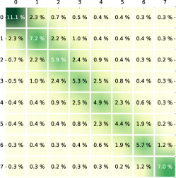
(c) $s=0.01$

Figure 7: Sparsification example using the Amazon-0312 graph.

Figure 7 illustrates the affect of the sparsification on the Amazon-0312 graph ($\sim$0.4 million vertices and $\sim$3 million directed edges). In this figure we plot the heat map of the Amazon-0312 graph when it is partitioned into $8\times 8$ uniform tiles for three cases; without sparsification, sparsification factor of $s=0.1$ (i.e., keeping $10\%$ of the nonzeros) and sparsification factor of $s=0.01$ (i.e., keeping $1\%$ of the nonzeros). We observe that when we only keep $10\%$ of the edges, nonzero distribution of the matrix is almost the same and there are slight changes when we keep only $1\%$ of the edges.

We can control expected relative error by automatically adjusting sparsification. For a given partitioned matrix, if there are $Z$ nonzeros in a tile, then the expected value is $Zs$, for the number of nonzeros after flipping, $Z^{\prime}$. $Z^{\prime}$ follows the binomial distribution, $Z^{\prime}\sim B(Z,s)$. The variance of the distribution of the number of nonzeros in a tile is $Zs(1-s)$. Thus, the expected relative error of the estimation of the nonzeros in the tile will be on the order of:

$$1-\epsilon \leq\frac{Z^{\prime}}{Zs}\leq 1+\epsilon,$$

$$\text{where}\;\epsilon \approx\frac{\sqrt{Zs(1-s)}}{Zs}=\sqrt{\frac{1-s}{Zs}}.$$

The above inequality implies that if a matrix has $m$ nonzeros, then under any given partition vector that divides the matrix into $p^{2}$ tiles, the maximum loaded tile will have at least $\frac{m}{p^{2}}$ nonzeros. Then, the relative error will be on the order of $\sqrt{(1-s)p^{2}/(ms)}$. For instance, if a matrix has $m=11\times 10^{6}$ nonzeros, the maximum loaded tile will have not less than $\frac{11\times 10^{6}}{64}\approx 1.7\times 10^{5}$ nonzeros under any $8\times 8$ ($p=8$) partitioning. If the probability $k$ we define for flipping coins is $0.1$, then the relative error will be around $0.007$. Hence, all the algorithms in this paper can be run on the sparsified matrix without significant change in the quality. Let $A^{\prime}$ be a sparsified version of the given matrix $A$ and $C$ be a partition vector. The related load imbalance formula can be defined as:

$$\lambda(A,C,C)= \frac{L_{max}\{A,C,C\}}{L_{avg}\{A,C,C\}}\text{ and }1-\epsilon\leq\frac{L_{max}\{A^{\prime},C,C\}}{L_{max}\{A,C,C\}\times s}\leq 1+\epsilon$$

$$\implies \frac{L_{max}\{A,C,C\}}{L_{avg}\{A,C,C\}}(1-\epsilon)\leq\frac{L_{max}\{A^{\prime},C,C\}}{L_{avg}\{A,C,C\}\times s}\leq\frac{L_{max}\{A,C,C\}}{L_{avg}\{A,C,C\}}(1+\epsilon)$$

$$\implies \lambda(A,C,C)(1-\epsilon)\leq\frac{L_{max}\{A^{\prime},C,C\}}{L_{avg}\{A,C,C\}\times s}\leq\lambda(A,C,C)(1+\epsilon)$$

Meaning that the load imbalance will be off on the order of $\epsilon$. From now on, we will call $\epsilon$ as error tolerance for automatic sparsification factor selection.

8 Implementation Details

We implemented our algorithms using C++ standard $17$ and compile our code-base with GCC version $9.2$. We have collected all of our implementations in a library we named SpatiAl Rectilinear Matrix pArtitioning (SARMA). Source code of SARMA is publicly available at http://github.com/GT-TDAlab/SARMA via a BSD-license. C++ added support for parallel algorithms to the standard library by integrating Intel’s TBB library starting from the standard $17$. Note that, in this work our goal is not parallelizing the partitioning framework, to provide better performance with the minimal work, in our code-base we simply enabled parallel execution policy of the standard library functions and parallelized pleasingly parallel loops wherever it is possible.

Figure 8 presents strong scaling speedup of Nic and PaL algorithms on $687$ graphs on an Intel architecture that have $24$ cores and no hyper-threading. In the plot, graphs are sorted based on their number of nonzeros on the x-axis. Adjacency matrices of graphs are partitioned into $32\times 32$ tiles. Achieved speedup is provided on the y-axis for each graph on different cores. In this experiment, we ran each algorithm $10$ times on $1$, $3$, $6$, $12$ and $24$ cores and report the median of the runs. As expected, we observe that achieved speedup increases with the graph size. The Nic algorithm achieves up-to $15$ times and PaL algorithm achieves up-to $17$ times speedup on $24$ cores. With small graphs we observe very limited speedups because these graphs can fit into the cache in the sequential case and parallelization does not compensate poor cache utilization.

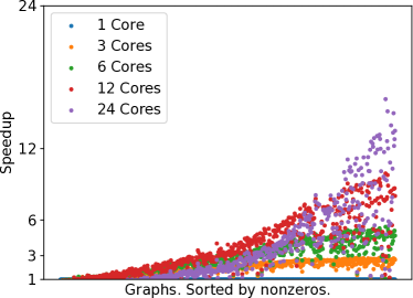
(a) Nicol’s algorithm.

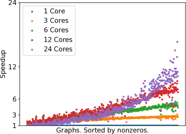
(b) PaL algorithm.

Figure 8: Strong scalability experiments on Nic and PaL algorithms. Graphs are sorted based on their nonzeros on the x-axis and partitioned as $32\times 32$. Number of cores: $\{1$, $3$, $6$, $12$, $24\}$

9 Experimental Evaluation

We ran our experiments on a $416$-node cluster owned by the Partnership for an Advanced Computing Environment (PACE) of Georgia Institute of Technology equipped with $2\times 12$ cores $2.7$ GHz Intel Xeon $6226$ CPUs, $192$ GB of RAM and at least $512$ GB of local storage. We ran each algorithm for $4$ different cuts, $p=\{4,8,16,32\}$ or $4$ different target loads, $Z=\{m/4,m/9,m/16,m/25\}$, and without sparsification and with $\epsilon=0.01$. We used the Moab scheduler along with the Torque resource manager that runs every partitioning algorithm one-by-one on a matrix on one of the available nodes.

We evaluated our algorithms on real-world and synthetic graphs from the SuiteSparse Matrix Collection [10]. We excluded non-square matrices and matrices that have less than $1$ million or more than $2$ billion nonzeros. There were $687$ matrices satisfying these properties (there were a total of $2,856$ matrices at the time of this experimentation). We also chose a subset of $16$ graphs from those graphs. Table 4 lists those graphs that we used in some of our experiments along with the graph name, origin/source of the graph, number of rows ($n$), number of nonzeros ($m$) and average number of nonzeros per row ($m/n$).

Table 4: Properties of the subset of our dataset along with their name, origin, number of rows ($n$), number of nonzeros ($m$) and average number of nonzeros per row ($m/n$).

Matrix Name	Matrix Origin	$\boldsymbol{n}$	$\boldsymbol{m}$	$\boldsymbol{m/n}$
wb-edu	Web	$9,845,725$	$57,156,537$	$5.8$
road_usa	Road	$23,947$,347	$57,708,624$	$2.4$
circuit5M	Simulation	$5,558,326$	$59,524,291$	$10.7$
soc-LiveJournal1	Social	$4,847,571$	$68,993,773$	$14.2$
kron_g500-logn20	Kronecker	$1,048,576$	$89,239,674$	$85.1$
dielFilterV3real	Electromagnetics	$1,102,824$	$89,306,020$	$81.0$
europe_osm	Road	$50,912,018$	$108,109,320$	$2.1$
hollywood-2009	Movie/Actor	$1,139,905$	$113,891,327$	$99.9$
Cube_Coup_dt6	Structural	$2,164,760$	$124,406,070$	$57.5$
kron_g500-logn21	Kronecker	$2,097,152$	$182,082,942$	$86.8$
nlpkkt160	Optimization	$8,345,600$	$225,422,112$	$27.0$
com-Orkut	Social	$3,072,441$	$234,370,166$	$76.3$
uk-2005	Web	$18,520,486$	$298,113,762$	$16.1$
stokes	Semiconductor	$11,449,533$	$349,321,980$	$30.5$
kmer_A2a	Biological	$170,728$,175	$360,585,172$	$2.1$
twitter	Social	$41,652,230$	$1,468,365,182$	$35.3$

We present some of our results using performance profiles [12]. In a performance profile plot, we show how bad a specific algorithm performs within a factor $\theta$ of the best algorithm that can be obtained by any of the compared algorithms in the experiment. Hence, the higher and closer a plot is to the y-axis, the better the method is.

9.1 Comparison with the optimal solution

To the best of our knowledge, this is the first work that tackles the symmetric rectilinear partitioning problem. Hence, we do not have a fair baseline. To understand the quality of the partitioning algorithms, in this experiment we compare Bull. astr. Inst. Czechosl.(PaL) algorithm’s load imbalance with the optimal solution. We implemented our mathematical model (as shown in Section 4.1) using Gurobi [18]. Since finding the optimal solution is computationally expensive, in addition to our dataset, we downloaded $375$ small graphs from SuiteSparse matrix collection [10] that have less than $9,000$ nonzeros. We partition those graphs into $8\times 8$ ($p=8$) tiles. Figure 9 illustrates the performance profile for the load-imbalance between the optimal solution and the Bull. astr. Inst. Czechosl.(PaL) algorithm. We observe that Bull. astr. Inst. Czechosl.(PaL) algorithm achieves the optimal solution on $67\%$ of the test instances and give nearly the optimal solution on $80\%$ of the test instances. At the worst case, the Bull. astr. Inst. Czechosl.(PaL) algorithm outputs at most $1.9$ times worse results than the optimal case.

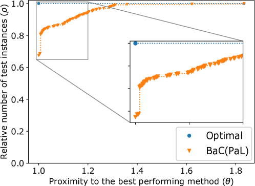
Figure 9: Comparison with the optimal solutions using a performance profile.

9.2 Experiments on the sample dataset

In the following experiments, we show raw load-imbalance and execution time results of different algorithms on chosen $16$ graphs under various settings. Later, we evaluate the effect of the sparsification on the load imbalance and the execution time. In those experiments, we consider Uni, Nic, RaC and Bull. astr. Inst. Czechosl.(PaL) algorithms for the mLI problem. For Uni, RaC, and Bull. astr. Inst. Czechosl.(PaL) algorithms, we choose $p=32$ and for the Nic algorithm, we choose $p=q=32$. Hence, every graph is partitioned into $32\times 32$ tiles. We ran experiments without sparsification, with $s=1\%$, $s=0.1\%$ and $\epsilon=0.01$. Note that $s$ is the sparsification factor and $\epsilon$ is the error tolerance for automatic sparsification factor selection.

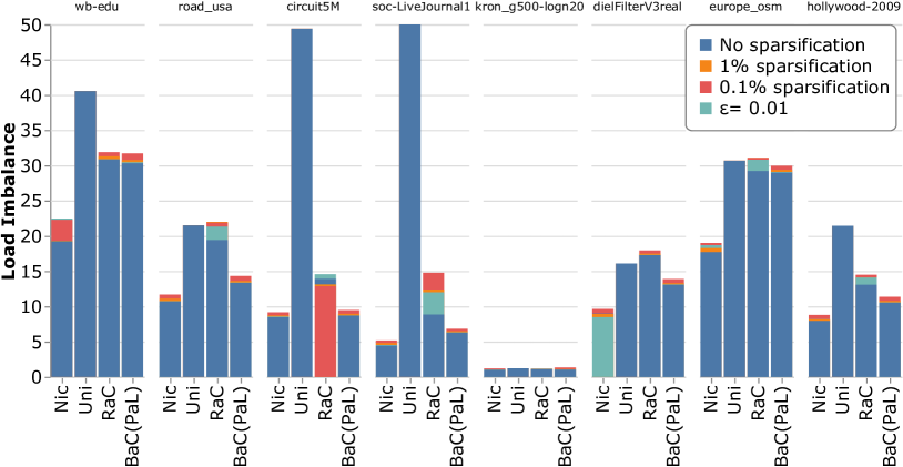
(a)

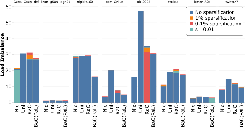
(b)

Figure 10: Load imbalance comparison on sample dataset.

9.2.1 Effect of sparsification on the load imbalance

Figure 10 reports load imbalances of four different algorithms; Uni, Nic, RaC, and Bull. astr. Inst. Czechosl.(PaL) on our selected $16$ graphs. In Figure 10, each bar presents the load imbalance for a graph instance. Blue bars represent the load imbalance when sparsification is off and others represent when sparsification is on. As expected, on majority of the cases, the Nic algorithm gives the best load imbalance. Because, symmetric rectilinear matrix partitioning is a very restricted problem and, being able to align different partition vectors to rows and columns gives a big flexibility to the Nic algorithm. Even with the restrictive nature, best of our symmetric partitioning algorithm gives no worse load imbalance than $1.7\times$ with-respect-to the Nic algorithm. Bull. astr. Inst. Czechosl.(PaL) algorithm gives the best performance among three symmetric partitioning algorithms on $15$ out of $16$ cases. Since rmat graphs have a well distributed matrix structure, we see that all algorithms give nearly optimal load imbalance on kronecker graphs. In the worst case, the RaC algorithm gives $\approx 1.8$ times worse load imbalance than the Bull. astr. Inst. Czechosl.(PaL) algorithm. As expected, the Uni algorithm performs poor on the majority of the matrices. Especially on the matrices that have skewed distributions such as soc-LiveJournal1 and uk-2005. Enabling sparsification mostly affects the RaC algorithm due to mapping of the problem from two-dimensional case to one-dimensional case and also applying the refinement on the same direction continuously. We observe almost negligible errors on the other algorithms (less than $0.005$). Note that, even for the RaC algorithm, error of the load imbalance is less than $0.01$ in the majority of graphs ($11$ out of $16$).

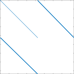
(a)

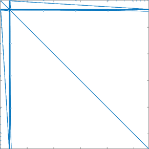
(b)

Figure 11: Sparsity patterns of nlpkkt160 and circuit5M matrices.

The sparsity pattern of a matrix may play a role on the final load imbalance. We observe that on our sample dataset the Uni partitioning gives better load imbalance than the RaC partitioning on dielFilterV3real and nlpkkt160 matrices when there is no sparsification. Besides, on stokes and kmer_A2a matrices the RaC algorithm only gives slightly better load imbalance than the Uni partitioning. Sparsity patterns of those matrices are the primary factor. To visualize, Figure 11 plots sparsity patterns of the nlpkkt160 (Figure 11a) and the circuit5M (Figure 11b) matrices. On the nlpkkt160 matrix the Uni algorithm, the Nic algorithm and the RaC algorithm outputs similar load imbalances. As illustrated in Figure 11a, the nlpkkt160 graph is really sparse and the pattern is three regular lines. Hence, refinement algorithm outputs poor partition vectors for both Nic and RaC. Since the pattern is regular Uni gives good load imbalance and Bull. astr. Inst. Czechosl.(PaL) algorithm outperforms the other algorithm by considering more possibilities on two-dimensional case. On the other hand, on the circuit5M matrix the Uni algorithm gives really poor load imbalance because that matrix have regular dense regions on the first set of beginning rows and columns as illustrated in Figure 11b. Due to this dense structure on that graph Bull. astr. Inst. Czechosl.(PaL) and Nic algorithms gives similar results because refinement algorithm tries to put more cuts to the beginning of the partition vectors.

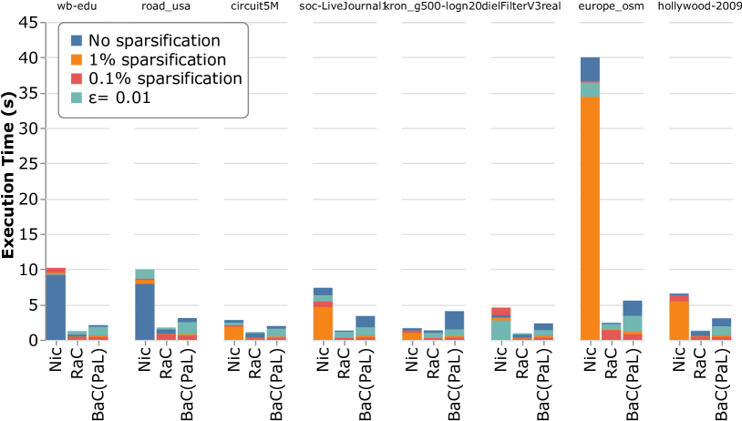
(a)

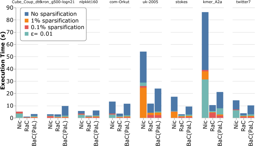
(b)

Figure 12: Execution time comparison on sample dataset.

9.2.2 Effect of sparsification on execution time

Figure 12 reports execution times of three different algorithms; Nic, RaC and Bull. astr. Inst. Czechosl.(PaL) on our selected $16$ graphs. We discard the Uni algorithm from this experiment since it can be computed in constant time. For the Bull. astr. Inst. Czechosl.(PaL) algorithm, the execution time includes the generation of the sparse-prefix-sum data structure. In Figure 12, each bar represents the execution time for a graph instance. Blue bar represents execution time when sparsification is off and the others represent when sparsification is on. As expected, on the majority of the test instances, the RaC algorithm gives the best execution time, because of its lighter computational complexity. The Nic algorithm is slower than Bull. astr. Inst. Czechosl.(PaL) and RaC algorithms up to $3.5\times$ and $7\times$ respectively. We observe that, sparsification decreases the Bull. astr. Inst. Czechosl.(PaL) algorithm’s execution time more than $2$ times (up to $12$ times) on majority of the test instances. The Bull. astr. Inst. Czechosl.(PaL) algorithm’s execution time is dominated by the set-up time of the sparse-prefix-sum data-structure. However, with sparsification, creation cost of sparse-prefix-sum data-structure decreases significantly. Since the complexity of Nic and RaC algorithms mostly depends on the number of rows ($n$) and number of cuts ($p$), the affect of the sparsification on those algorithms are less significant. With sparsification, we observe decreases in their execution time from $1.2\times$ to $2.5\times$.

Experiments above show that without loss of quality, sparsification significantly improves partitioning algorithms performance.

9.3 Evaluation of the load imbalance

In this section, we evaluate the quality of the partition vectors that our proposed algorithms output in terms of load imbalance on our complete dataset. We run RaC and Bull. astr. Inst. Czechosl.(PaL) algorithms where $p=\{4,8,16,32\}$ and we run PaL and BaL (RaC) algorithms where $Z=\{m/4,m/9,m/16,m/25\}$. In the following experiments, we also include Uni and BaL (Uni) algorithms as baselines.

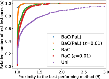
(a) $4\times 4$

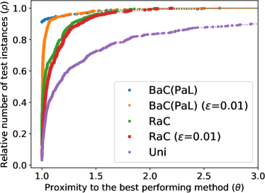
(b) $8\times 8$

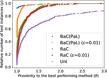
(c) $16\times 16$

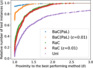
(d) $32\times 32$

Figure 13: Load imbalance comparison using performance profiles (mLI problem).

9.3.1 Load imbalance on the mLI problem

We evaluate relative load imbalance performances of RaC, Bull. astr. Inst. Czechosl.(PaL) and Uni algorithms. The aim is to illustrate the efficiency of the proposed algorithms with respect to the Uni algorithm. In this experiment, we choose $p=\{4,8,16,32\}$ and we report results without sparsification and with sparsification where the error tolerance for automatic sparsification factor selection is set to; $\epsilon=0.01$. Figure 13 illustrates the performance profiles of the algorithms for different $p$ values. Note that, in the performance profiles, we plot how bad a specific algorithm performs within a factor $\theta$ of the best algorithm. We observe that in all test instances (Figures 13a and 13d) Bull. astr. Inst. Czechosl.(PaL) algorithm gives the best performance. RaC algorithm is the second-best algorithm and in the worst case, it outputs a partition vector that gives less than $3$ times worse load-imbalance when $p=32$ with respect to the best algorithm. We observe that number of test instances where sparsification does not change the Bull. astr. Inst. Czechosl.(PaL) algorithm’s output increases for larger $p$ values. For instance, when $p=32$, in $\approx 70\%$ of the test instances that run on sparsified instances gives the same load imbalance as non-sparsified instances. This ratio is $\approx 35\%$ when $p=4$. On the other hand, with sparsification when $\epsilon$ is set to $0.01$, we observe that RaC algorithm performs slightly worse. This was expected because the RaC algorithm maps two-dimensional problem into one dimension hence it is more error prone.

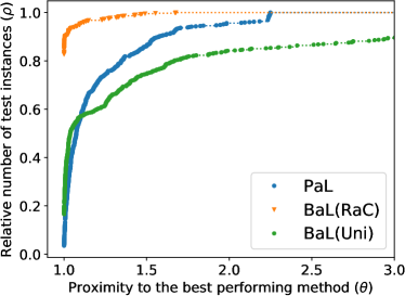
(a) $Z=m/4$

(b) $Z=m/9$

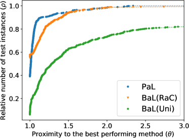
(c) $Z=m/16$

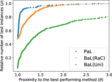
(d) $Z=m/25$

Figure 14: Load imbalance comparison using performance profiles (mNC problem).

9.3.2 Load imbalance on the mNC problem

We evaluate relative load imbalance performances of PaL, BaL (RaC) and BaL (Uni) algorithms. The aim is to illustrate the efficiency of the proposed algorithms with respect to the BaL (Uni) algorithm. In this experiment, we choose $Z=\{m/4,m/9,m/16,m/25\}$ and we report results without sparsification because sparsification may cause bigger errors in the mNC problem. Figure 14 illustrates the performance profiles of the algorithms for different $Z$ values. We observe that when $Z$ is larger (see Figures 14a and 14b) The BaL (RaC) algorithm performs slightly better than PaL algorithm. The PaL algorithm outperforms for smaller $Z$ values (see Figure 14c).

9.4 Evaluation of the partitioning time

In this section we evaluate the execution times of the algorithms that we proposed for mLI and mNC problems on our complete dataset. Reported execution times include sparsification time, sparse-prefix-sum data-structure construction time, and partitioning time. We run RaC and Bull. astr. Inst. Czechosl.(PaL) algorithms where $p=\{4,8,16,32\}$ and we run PaL and BaL (RaC) algorithms where $Z=\{m/4,m/9,m/16\}$. In the following experiments we also include Uni and BaL (Uni) algorithms as baselines. In the following experiments we report the median of $10$ runs for each test instance.

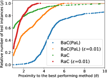
(a) $4\times 4$

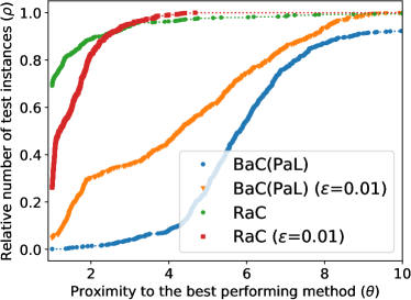
(b) $8\times 8$

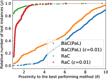
(c) $16\times 16$

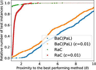
(d) $32\times 32$

Figure 15: Execution time comparison using performance profiles (mLI problem).

9.4.1 Partitioning time on the mLI problem

We evaluate relative executions times of RaC and Bull. astr. Inst. Czechosl.(PaL) algorithms. In this experiment, we choose $p=\{4,8,16,32\}$ and we report results without sparsification and with sparsification where the load imbalance error is set to be off on the order of one percent; $\epsilon=0.01$. Figure 13 illustrates the performance profiles of the algorithms for different $p$ values. We observe that in all cases (Figures 15a and 15d) as expected, RaC algorithm gives the best execution time, because of its lighter computational complexity. The Bull. astr. Inst. Czechosl.(PaL) algorithm’s execution time is decreases significantly when the sparsification is on. In overall, sparsification slightly improves the RaC algorithms execution time because the gain in the partitioning time do not compensate the sparsification time for smaller graphs .

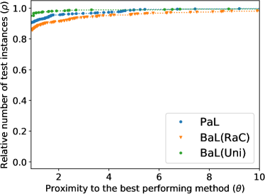
(a) $Z=m/4$

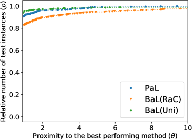
(b) $Z=m/9$

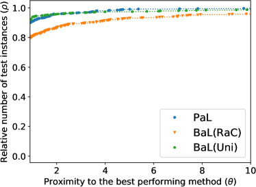
(c) $Z=m/16$

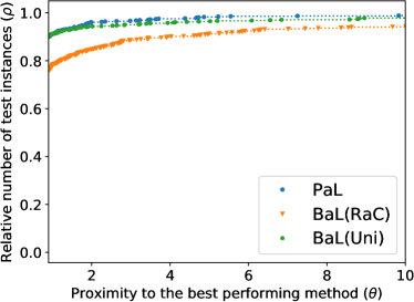
(d) $Z=m/25$

Figure 16: Execution time comparison using performance profiles (mNC problem).

9.4.2 Partitioning time on the mNC problem

We evaluate relative execution time performances of PaL, BaL (RaC), and BaL (Uni) algorithms. The aim is to illustrate the efficiency of the proposed algorithms with respect to the Uni algorithm. In this experiment, we choose $Z=\{m/4,m/9,m/16\}$ and we report results without sparsification because sparsification may cause bigger errors in the mNC problem. Figure 16 illustrates the performance profiles of the algorithms for different $Z$ values. We observe that, in all instances the PaL algorithm outperforms the other algorithms. Because, both BaL (RaC) and BaL (Uni) algorithms do many tests for different target cuts and load lookups. Hence, their computational complexities are higher than the PaL algorithm.

10 Conclusion

In this paper, we show that the optimal solution to the symmetric rectilinear partitioning is NP-Hard, and we propose refinement-based and probe-based heuristic algorithms to two variants of this problem. After providing complexity analysis of the algorithms, we implement a data-structure and sparsification strategies to reduce the complexities. Our experimental evaluation shows that our proposed algorithms are very efficient to find good-quality solutions, such that we achieve a nearly optimal solution on $80\%$ instances of 375 small graphs. We also open source our code at http://github.com/GT-TDAlab/SARMA for public usage and future development.

As future work, we are working on decreasing the space requirements of our sparse prefix sum data structure. In addition, we will also investigate approximation techniques, and parallelization of the proposed algorithms.

References

- [1] S. Balay, W. D. Gropp, L. C. McInnes, and B. F. Smith, Efficient management of parallelism in object oriented numerical software libraries, in Modern Software Tools in Scientific Computing, E. Arge, A. M. Bruaset, and H. P. Langtangen, eds., Birkhäuser Press, 1997, pp. 163–202.
- [2] N. Bell and M. Garland, Implementing sparse matrix-vector multiplication on throughput-oriented processors, in Proceedings of the conference on high performance computing networking, storage and analysis, 2009, pp. 1–11.
- [3] M. Benzi, Preconditioning techniques for large linear systems: a survey, Journal of computational Physics, 182 (2002), pp. 418–477.
- [4] M. J. Berger and S. H. Bokhari, A partitioning strategy for nonuniform problems on multiprocessors, IEEE Transactions on Computers, (1987), pp. 570–580.
- [5] E. G. Boman, K. D. Devine, and S. Rajamanickam, Scalable matrix computations on large scale-free graphs using 2d graph partitioning, in SC’13: Proceedings of the International Conference on High Performance Computing, Networking, Storage and Analysis, 2013, pp. 1–12.
- [6] L. Buatois, G. Caumon, and B. Levy, Concurrent number cruncher: a gpu implementation of a general sparse linear solver, International Journal of Parallel, Emergent and Distributed Systems, 24 (2009), pp. 205–223.
- [7] E. Cáceres, F. Dehne, A. Ferreira, P. Flocchini, I. Rieping, A. Roncato, N. Santoro, and S. W. Song, Efficient parallel graph algorithms for coarse grained multicomputers and bsp, in International Colloquium on Automata, Languages, and Programming, Springer, 1997, pp. 390–400.
- [8] Ü. V. Çatalyürek and C. Aykanat, Hypergraph-partitioning based decomposition for parallel sparse-matrix vector multiplication, IEEE Transactions on Parallel and Distributed Systems, 10 (1999), pp. 673–693.
- [9] Ü. V. Çatalyürek, C. Aykanat, and B. Uçar, On two-dimensional sparse matrix partitioning: Models, methods, and a recipe, SIAM Journal on Scientific Computing (SISC), 32 (2010), pp. 656–683.
- [10] T. A. Davis and Y. Hu, The University of Florida sparse matrix collection, ACM Transactions on Mathematical Software (TOMS), (2011), p. 1.
- [11] T. A. Davis, S. Rajamanickam, and W. M. Sid-Lakhdar, A survey of direct methods for sparse linear systems, Acta Numerica, 25 (2016), pp. 383–566.
- [12] E. D. Dolan and J. J. Moré, Benchmarking optimization software with performance profiles, Mathematical programming, 91 (2002), pp. 201–213.
- [13] J. R. Driscoll, N. Sarnak, D. D. Sleator, and R. E. Tarjan, Making data structures persistent, in Proceedings of the eighteenth annual ACM symposium on Theory of computing, 1986, pp. 109–121.
- [14] P. M. Fenwick, A new data structure for cumulative frequency tables, Software: Practice and Experience, 24 (1994), pp. 327–336.
- [15] M. Garland, Sparse matrix computations on manycore gpu’s, in Proceedings of the 45th annual Design Automation Conference, 2008, pp. 2–6.
- [16] A. George, J. R. Gilbert, and J. W. Liu, Graph theory and sparse matrix computation, vol. 56, Springer Science & Business Media, 2012.
- [17] M. Grigni and F. Manne, On the complexity of the generalized block distribution, in International Workshop on Parallel Algorithms for Irregularly Structured Problems, 1996, pp. 319–326.
- [18] L. Gurobi Optimization, Gurobi optimizer reference manual, 2020, http://www.gurobi.com.
- [19] B. Hendrickson and T. G. Kolda, Graph partitioning models for parallel computing, Parallel computing, 26 (2000), pp. 1519–1534.
- [20] B. Hendrickson, R. Leland, and S. Plimpton, An efficient parallel algorithm for matrix-vector multiplication, International Journal of High Speed Computing, 7 (1995), pp. 73–88.
- [21] M. A. Heroux, R. A. Bartlett, V. E. Howle, R. J. Hoekstra, J. J. Hu, T. G. Kolda, R. B. Lehoucq, K. R. Long, R. P. Pawlowski, E. T. Phipps, et al., An overview of the trilinos project, ACM Transactions on Mathematical Software (TOMS), 31 (2005), pp. 397–423.
- [22] S. Hong, T. Oguntebi, and K. Olukotun, Efficient parallel graph exploration on multi-core cpu and gpu, in 2011 International Conference on Parallel Architectures and Compilation Techniques, IEEE, 2011, pp. 78–88.
- [23] E.-J. Im, K. Yelick, and R. Vuduc, Sparsity: Optimization framework for sparse matrix kernels, The International Journal of High Performance Computing Applications, 18 (2004), pp. 135–158.
- [24] J. JaJa, C. W. Mortensen, and Q. Shi, Space-efficient and fast algorithms for multidimensional dominance reporting and counting, in Algorithms and Computation, Springer Berlin Heidelberg, 2005, pp. 558–568.
- [25] G. Karypis and V. Kumar, A fast and high quality multilevel scheme for partitioning irregular graphs, SIAM Journal on scientific Computing, 20 (1998), pp. 359–392.
- [26] J. Kepner, P. Aaltonen, D. Bader, A. Buluç, F. Franchetti, J. Gilbert, D. Hutchison, M. Kumar, A. Lumsdaine, H. Meyerhenke, et al., Mathematical foundations of the graphblas, in 2016 IEEE High Performance Extreme Computing Conference (HPEC), IEEE, 2016, pp. 1–9.
- [27] S. Khanna, S. Muthukrishnan, and S. Skiena, Efficient array partitioning, in International Colloquium on Automata, Languages, and Programming, 1997, pp. 616–626.
- [28] J. G. Lewis, D. G. Payne, and R. A. van de Geijn, Matrix-vector multiplication and conjugate gradient algorithms on distributed memory computers, in Proceedings of IEEE Scalable High Performance Computing Conference, IEEE, 1994, pp. 542–550.
- [29] Y. Lu, J. Cheng, D. Yan, and H. Wu, Large-scale distributed graph computing systems: An experimental evaluation, Proceedings of the VLDB Endowment, 8 (2014), pp. 281–292.
- [30] F. Manne and T. Sørevik, Partitioning an array onto a mesh of processors, in International Workshop on Applied Parallel Computing, 1996, pp. 467–477.
- [31] D. Meagher, Geometric modeling using octree encoding, Computer graphics and image processing, 19 (1982), pp. 129–147.
- [32] D. M. Nicol, Rectilinear partitioning of irregular data parallel computations, Journal of Parallel and Distributed Computing, 23 (1994), pp. 119–134.
- [33] J. R. Pilkington and S. B. Baden, Dynamic partitioning of non-uniform structured workloads with spacefilling curves, IEEE Transactions on Parallel and Distributed Systems, 7 (1996), pp. 288–300.
- [34] A. Pınar and C. Aykanat, Fast optimal load balancing algorithms for 1D partitioning, Journal of Parallel and Distributed Computing, 64 (2004), pp. 974–996.
- [35] M. J. Quinn and N. Deo, Parallel graph algorithms, ACM Computing Surveys (CSUR), 16 (1984), pp. 319–348.
- [36] E. Saule, E. O. Bas, and Ü. V. Çatalyürek, Load-balancing spatially located computations using rectangular partitions, Journal of Parallel and Distributed Computing, 72 (2012), pp. 1201–1214.
- [37] X. Shi, Z. Zheng, Y. Zhou, H. Jin, L. He, B. Liu, and Q.-S. Hua, Graph processing on gpus: A survey, ACM Computing Surveys (CSUR), 50 (2018), pp. 1–35.
- [38] R. E. Tarjan and U. Vishkin, An efficient parallel biconnectivity algorithm, SIAM Journal on Computing, 14 (1985), pp. 862–874.
- [39] M. Ujaldon, S. D. Sharma, E. L. Zapata, and J. Saltz, Experimental evaluation of efficient sparse matrix distributions, in International Conference on Supercomputing, 1996, pp. 78–85.
- [40] A. Yaşar, S. Rajamanickam, J. W. Berry, M. M. Wolf, J. Young, and Ü. V. Çatalyürek, Linear algebra-based triangle counting via fine-grained tasking on heterogeneous environments, in IEEE High Performance Extreme Computing Conference (HPEC), 2019.