Rotation by shape change, autonomous molecular motors
and effective timecrystalline dynamics

Abstract

A deformable body can rotate even with no angular momentum, simply by changing its shape. A good example is a falling cat, how it maneuvers in air to land on its feet. Here a first principles molecular level example of the phenomenon is presented. For this the thermal vibrations of individual atoms in an isolated cyclopropane molecule are simulated in vacuum and at ultralow internal temperature values, and the ensuing molecular motion is followed stroboscopically. It is observed that in the limit of long stroboscopic time steps the vibrations combine into an apparent uniform rotation of the entire molecule even in the absence of angular momentum. This large time scale rotational motion is then modeled in an effective theory approach, in terms of timecrystalline Hamiltonian dynamics. The phenomenon is a temperature sensitive measurable. As such it has potential applications that range from models of autonomous molecular motors to development of molecular level detector, sensor and control technologies.

I Introduction

Geometric mechanics states that in the case of a deformable body, the vibrational and rotational motions are not separable Guichardet-1984 ; Shapere-1989a ; Shapere-1989b ; Littlejohn-1997 ; Marsden-1997 ; Katz-2019 ; Dai-2020b . Even with no angular momentum, local vibrations in parts of the body can become self-organized into an emergent, global rotation of the entire body. This effect is already used for a variety of control purposes, for example the attitude of satellites is often controlled by periodic motions of parts of a satellite such as spinning rotors Marsden-1997 .

Here the first molecular level realization of such an effective rotational motion is presented. The example describes how a molecule employs thermal (or quantum) fluctuations of its individual atoms to rotate akin a molecular motor, even when the molecule does no carry any angular momentum. For this kind of an effective rotational motion to emerge, the molecule needs to have at least three movable components Guichardet-1984 . A good example that is described here, is a single cyclopropane (C₃H₆) molecule. It is a ring molecule that is made of three methylenes (CH₂) at the corners of an equilateral triangle. As such, cyclopropane is the simplest example of an organic ring molecule. It is being studied widely, as a building block of organic synthesis. In medicine cyclopropane is also used extensively as an anesthetics Schneider-2014 ; Kulinkovich-2015 .

Other examples of simple triangular molecules that can be analyzed similarly include aziridine, oxirane and 1,2 dimethylcyclopropane Reddy-2018 .

II Theory

To understand the geometric provenance of deformation induced rotation Guichardet-1984 , consider the (time) $t$-evolution of three equal mass pointlike objects, at the corners $\mathbf{r}_{i}$ ($i=1,2,3$) of a triangle. There are no external forces, thus the center of mass is stationary at all times

$$\mathbf{r}_{1}(t)+\mathbf{r}_{2}(t)+\mathbf{r}_{3}(t)=0$$ (1)

The total angular momentum also vanishes

$$\mathbf{L}\ =\ \mathbf{r}_{1}\wedge\dot{\mathbf{r}}_{1}+\mathbf{r}_{2}\wedge\dot{\mathbf{r}}_{2}+\mathbf{r}_{3}\wedge\dot{\mathbf{r}}_{3}\ =\ 0$$ (2)

Nevertheless the triangle can rotate, by shape changes. To describe this rotation, the triangle is oriented to always lie on the $z=0$ plane; two triangles have the same shape when they only differ by a rigid rotation on the plane, around the $z$-axis. The shape is described by assigning internal shape coordinates $\mathbf{s}_{i}(t)$ to the three corners. These coordinates describe all possible triangular shapes in an unambiguous fashion when one demands that $\mathbf{s}_{1}(t)$ always coincides with the positive $x$-axis so that $s_{1x}(t)>0$ and $s_{1y}(t)=0$, and one sets $s_{2y}(t)>0$. The components of $\mathbf{s}_{3}(t)$ are determined as in (1),

$$\mathbf{s}_{3}(t)=-\mathbf{s}_{1}(t)-\mathbf{s}_{2}(t)$$

Now let the $\mathbf{s}_{i}(t)$ evolve arbitrarily, but in a $T$-periodic manner

$$\mathbf{s}_{i}(t+T)=\mathbf{s}_{i}(t)$$

The triangular shape then traces a closed loop $\Gamma$ in the space of all possible triangular shapes. At each time the shape coordinates $\mathbf{s}_{i}(t)$ relate to the space coordinates $\mathbf{r}_{i}(t)$ by a spatial rotation on the $z=0$ plane,

$$\left(\begin{array}[]{c}r_{ix}(t)\\ r_{iy}(t)\end{array}\right)=\left(\begin{array}[]{cc}\cos\theta(t)&-\sin\theta(t)\\ \sin\theta(t)&\ \cos\theta(t)\end{array}\right)\left(\begin{array}[]{c}s_{ix}(t)\\ s_{iy}(t)\end{array}\right)$$ (3)

Initially $\theta(0)=0$ so that whenever $\theta(\mathrm{T})\not=0$ the triangle has rotated. This rotation angle is evaluated by substituting (3) into (2):

$$\theta(\mathrm{T})\ =\ \int\limits_{0}^{\mathrm{T}}\!dt\,\,\frac{\sum\limits_{i=1}^{3}\left\{s_{iy}\dot{s}_{ix}-s_{ix}\dot{s}_{iy}\right\}}{\sum\limits_{i=1}^{3}\mathbf{s}^{2}_{i}}\ \equiv\ \int_{\Gamma}d{\mathbf{l}}\cdot{\mathbf{A}}$$ (4)

Whenever (4) does not vanish the triangle returns to its initial shape but with a net rotation by $\theta(\mathrm{T})\not=0$ around the axis through its center of mass. Since there is no angular momentum the rotation is emergent, it is entirely due to shape changes.

In (4) the angle has also been expressed as a line integral of a connection one-form $\mathbf{A}$ Guichardet-1984 ; Shapere-1989a ; Shapere-1989b ; Littlejohn-1997 ; Marsden-1997 ; Katz-2019 ; Dai-2020b . To identify it, start from Jacobi coordinates

$$\begin{array}[]{ccc}\mathbf{s}_{1}&=&\frac{1}{\sqrt{2}}\mathbf{u}-\frac{1}{\sqrt{6}}\mathbf{v}\\ \mathbf{s}_{2}&=&\sqrt{\frac{2}{3}}\mathbf{v}\\ \mathbf{s}_{3}&=&-\frac{1}{\sqrt{2}}\mathbf{u}-\frac{1}{\sqrt{6}}\mathbf{v}\end{array}$$

With

$$\left(\begin{matrix}u_{1}\\ u_{2}\end{matrix}\right)=r\cos\frac{\vartheta}{2}\left(\begin{matrix}\cos\phi_{1}\\ \sin\phi_{1}\end{matrix}\right)\ \ \ \&\ \ \ \left(\begin{matrix}v_{1}\\ v_{2}\end{matrix}\right)=r\sin\frac{\vartheta}{2}\left(\begin{matrix}\cos\phi_{2}\\ \sin\phi_{2}\end{matrix}\right)$$

and with

$$\phi_{\pm}=\phi_{1}\pm\phi_{2}$$

the connection one-form $\mathbf{A}$ becomes

$$\mathbf{A}=-\frac{1}{2}\cos\vartheta d\phi_{-}-\frac{1}{2}d\phi_{+}=\frac{1}{2}\frac{\ xdy-ydx}{r(r+z)}-\frac{1}{2}d(\phi_{+}+\phi_{-})$$ (5)

Remarkably $\mathbf{A}$ is akin the connection one-form of a Dirac monopole at the origin $r=0$ of $\mathbb{R}^{3}$ with the Dirac string placed along the negative $z$-axis. Thus (4) evaluates the flux of the monopole through a surface with boundary $\Gamma$ in the space of triangular shapes. Such a flux is generically nonvanishing so that $\theta(\mathrm{T})\not=0$ generically.

Notably, the Dirac string concurs with a shape where two corners overlap, and at the location of the monopole all three corners of the triangle coincide.

III Simulation results

In the case of a cyclopropane molecule the angle of rotation (4) can be evaluated numerically, using state-of-the-art all-atom classical molecular dynamics. This is a methodology that is designed for a realistic, accurate description of a molecular system at a semiclassical level. The simulation results presented here are obtained using the GROMACS package gromacs with CHARMM36m force field charmm36m in combination with CGenFF Vanommeslaeghe-2010 ; Vanommeslaeghe-2012 for parameter generation (simulation details are described in Appendix). The boundary conditions are free and both Coulomb and Van der Waals interactions extend over all atom pairs in the molecule, with no cut-off approximation. The initial cyclopropane structure is taken from the PubChem web-site PubChem . It has $\mathrm{D}_{3h}$ molecular symmetry, with atomic coordinates that are specified with $10^{-14}\ m$ precision. This approximates the minimum of the CHARMM36m potential energy with a precision that even exceeds its intended accuracy.

A set of 50 “random” initial configurations for the production runs is first constructed, by energy drift gromacs using single precision floating point format. Each initial configuration has a different internal molecular temperature value $T$ below $1.0$K that is determined by the equipartition theorem. The pool of initial configurations is designed to minimize the mechanical CHARMM36m free energy at the given internal temperature value $T$, with single precision floating point format. In particular, the angular momentum of each initial configuration vanishes with comparable numerical accuracy.

In the production runs double precision floating point format is used in combination with $\Delta\tau=1.0f$s time steps, which is quite standard in high precision all-atom simulations: This is sufficient to stabilize the internal molecular temperature so that $T$ remains essentially constant during each of the production runs, with vanishingly small energy drift. Each of the 50 production run trajectories simulate 10$\mu$s in silico and a single trajectory takes about 90 hours of wall clock time with the available processors.

It is verified that the angular momentum remains vanishingly small during all of the production runs. For this, the instantaneous positions and velocities of all the individual C and H atoms are recorded at every femtosecond time step $n$ of all production run trajectories. The instantaneous values $L_{z}(n)$ of angular momentum component that is normal to the plane of the three carbon atoms is evaluated for the entire molecule, together with the corresponding instantaneous moment of inertia values $I(n)$. This yields the instantaneous angular velocity values

$$\omega(n)=L_{z}(n)/I(n)$$

These instantaneous values $\omega(n)$ are summed up, to compute the accumulated “rigid body” rotation angle, that is due to angular momentum:

$$\vartheta(n)=\omega(n)\Delta\tau+\vartheta(n-1)\ =\ \sum\limits_{i=1}^{n}\frac{L_{z}(i)}{I(i)}\Delta\tau$$ (6)

In full compliance with the condition (2), in all the production run simulations the values of (6) always remain less than $\sim 10^{-6}$ radians, for all time steps $n$ and Figure 1 shows a typical example: In the production simulations there is no observable rotation of the cyclopropane molecule, due to angular momentum. Accordingly any systematic rotational motion that exceeds $\sim 10^{-6}$ radians during a production run must be emergent, and entirely due to shape deformations.

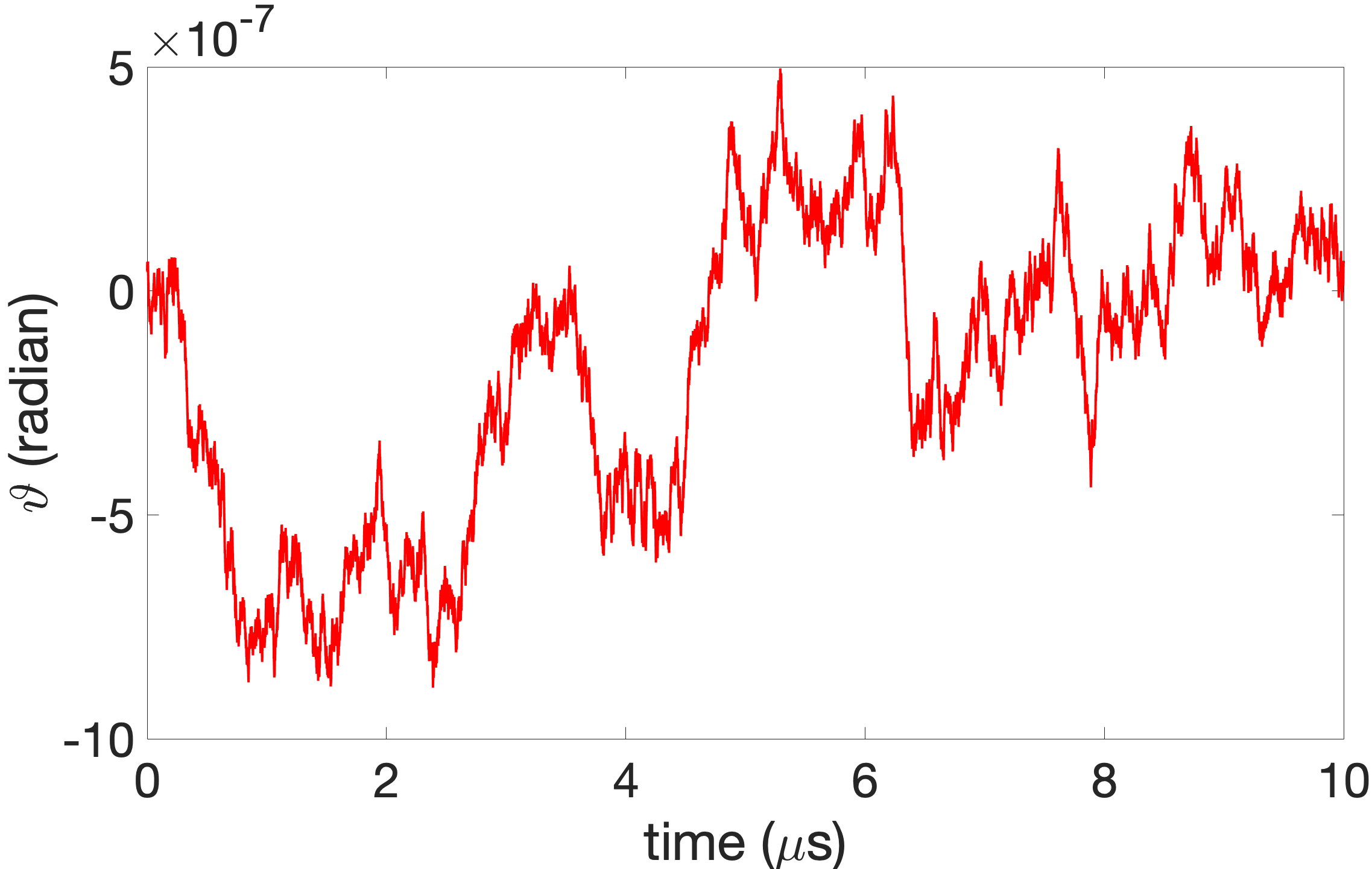
Figure 1: Generic time evolution of the angle $\vartheta(n)$ in equation (6) in the production runs: There is no observable net rotation due to angular momentum. In this example the internal temperature is $T=0.065$K and the same trajectory is analyzed in Figures 3.

To observe such a systematic rotational motion the orientation of the cyclopropane structure is monitored stroboscopically, using time steps that are large in comparison to the frequency of a typical covalent bond oscillation. It is found that the cyclopropane molecule always rotates, and the rotation is always around the center of mass axis that is normal to the plane of the three carbon atoms. Moreover, the angular velocity of the effective rotational motion is very sensitive to the value $T$ of internal molecular temperature.

In Figures 2 three different, generic examples of production run trajectories are presented; movies of these trajectories are available as Supplementary Material. In each trajectory, the molecule is observed with 100$p$s stroboscopic time steps.

In Figure 2 a) the internal molecular temperature has the value $T=0.066$K. The molecule rotates in a uniform fashion clockwise i.e. with increasing $\theta(t)$ at a constant rate of $\sim$10 rad/$\mu$s around the axis that is normal to the plane of the carbon. In Figure 2 b) $T=0.0087$K. Now the rotational motion is ratcheting, with a drift towards decreasing values of $\theta(t)$ at around $\sim$0.07 rad/$\mu$s. Such a combination of ratcheting and drifting motion is quite commonly observed, at low $T$-values and with those relatively short stroboscopic time steps that are attainable in the simulations. The drift implies that with larger stroboscopic time steps, in excess of 10$\mu$s which is the length of a production trajectory, the rotation becomes increasingly uniform; this will be exemplified in Figures 3. Finally, in Figure 2 c) $T=0.94$K which is close to the upper bound of $T$-values accessible in the present simulations, while maintaining a good numerical stability. Now the molecule rotates in the counterclockwise direction at a rate around $\sim$15 rad/$\mu$s during the 10$\mu$s simulation. The rotation remains slightly erratic at the stroboscopic time scale. Presumably, an increase in the stroboscopic time scale in combination with a longer MD trajectory produces a uniform rotation also in this case.

Unfortunately, with the available computers it is not feasible to try and produce trajectories that are much longer than 10$\mu$s, with a high level of numerical stability. Such trajectories would be needed, to analyze in detail higher $T$-values. The present simulation results propose that there is a critical value $T_{c}$ probably around a few Kelvin, above which uniform stroboscopic rotation can no longer be observed. This could be a consequence of simulation artifacts that are due to issues such as energy drift gromacs .

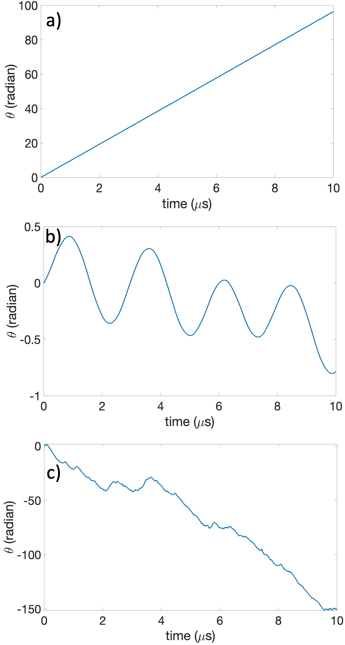
Figure 2: Evolution of rotation angle (4) in cyclopropane, at different internal $T$-values and stroboscopic time step $\Delta t=10^{-10}$s. In Figure a) $T=0.066$K, in Figure b) $T=0.0087$K, in Figure c) $T=0.94$K. See Supplementary material.

In Figures 3 the trajectory shown in Figure 1 is analyzed in more detail; the internal temperature value $T=0.065$K in this Figure is very close to the $T$-value of the trajectory in Figure 2 a).

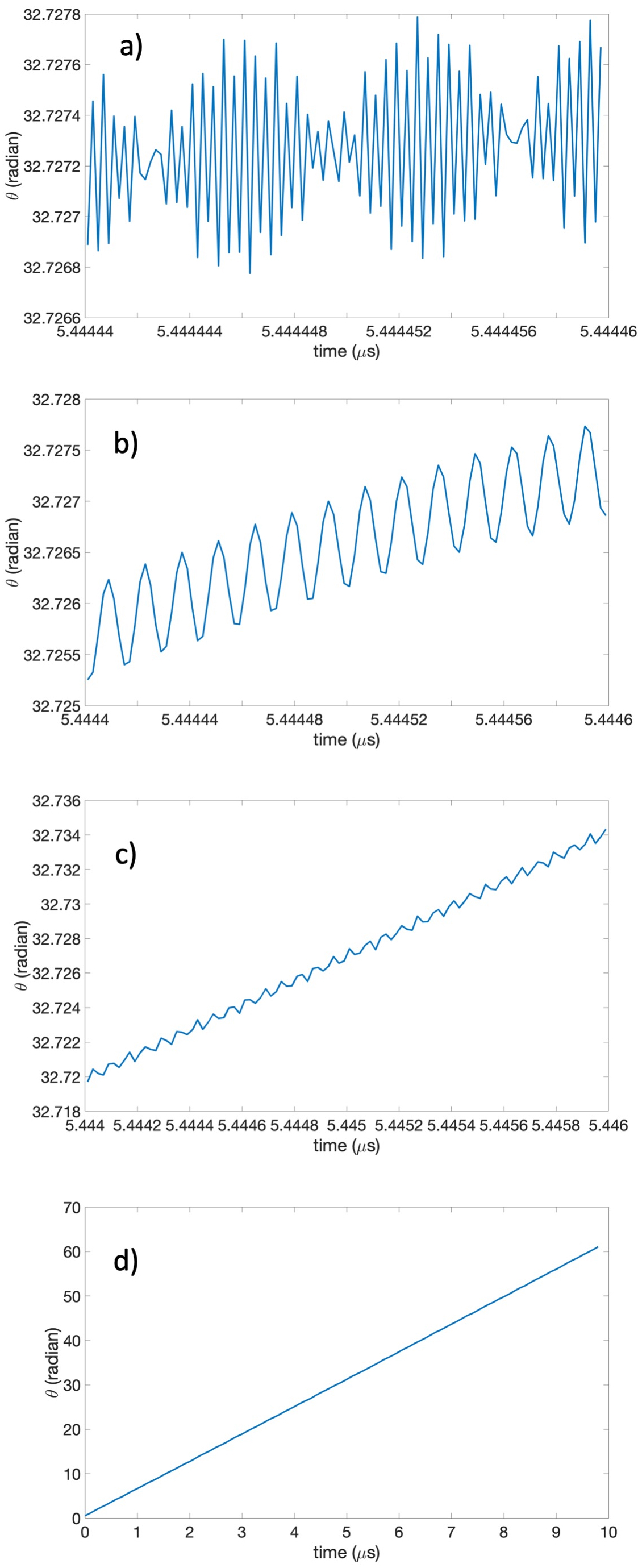
Figure 3: Time evolution of rotation angle $\theta(t)$ along a $T=0.065$K trajectory sampled different stroboscopic time steps $\Delta t$. In Figure a) $\Delta t=10^{-13}$ s, in Figure b) $\Delta t=10^{-12}$s, in Figure c) $\Delta t=10^{-11}$s and in Figure d) $\Delta t=10^{-7}$s.

In Figure 3 a) $\theta(t)$ is sampled with very short stroboscopic time steps $\Delta t=200$$f$s. Oscillatory rotational motion is observed, with an amplitude that also oscillates but at much lower frequency. In Figures 3 b) and 3 c) the time steps are increased to $\Delta t=2.0$$p$s and $\Delta t=20$$p$s, respectively. Now an increasingly regular ratcheting motion is observed, with apparent clockwise rotation, and with a decreasing relative amplitude; see also Figure 2 b). Finally, in Figure 3 d) where $\Delta t=100n$s the cyclopropane structure apparently rotates and in a uniform manner, akin the rotational motion shown in Figure 2 a). Despite a very small difference in $T$-values, the angular velocity is now clearly slower. Indeed, a peak of angular velocity that is centered at $T\approx 0.066$K is very narrow. Thus the rotational motion is a very sensitive measurable.

IV Effective theory analysis

The Figures 3 demonstrate how an emergent separation of scales leads to a dynamical self-organization as the stroboscopic time steps increase. In the final Figure 3 d) the cyclopropane rotates like an equilateral triangle, in a uniform fashion at constant angular velocity, around the symmetry axis that is normal to the plane of the three methylenes. This emergent uniform rotation has all the characteristics of energy conserving, Hamiltonian dynamics. As such, it can be described by an effective Hamiltonian theory in terms of a reduced set of variables, appropriate to govern the molecule in the limit of large stroboscopic time steps. It is apparent that this effective theory must coincide with the timecrystalline Hamiltonian model analyzed in Dai-2019 ; Alekseev-2020 ; Dai-2020b . This is an effective theory that describes the time evolution of three point-like interaction centers $\mathbf{x}_{1},\mathbf{x}_{2}$ and $\mathbf{x}_{3}$ in terms of the three link vectors

$$\mathbf{n}_{i}=\mathbf{x}_{i+1}-\mathbf{x}_{i}$$

with $\mathbf{x}_{4}=\mathbf{x}_{1}$ that are subject to the Lie-Poisson brackets

$$\{n^{a}_{i},n^{b}_{j}\}=\pm\delta_{ij}\epsilon^{abc}n^{c}_{i}$$

where the two signs are related by parity. Hamilton’s equation is

$$\frac{\partial\mathbf{n}_{i}}{\partial t}\ =\ \{\mathbf{n}_{i},H(\mathbf{n})\}\ =\ \mp\mathbf{n}_{i}\times\frac{\partial H}{\partial\mathbf{n}_{i}}$$ (7)

Since

$$\{n^{a}_{i},\mathbf{n}_{j}\cdot\mathbf{n}_{j}\}=0$$

for all $i,j$ the bracket preserves the length of $\mathbf{n}_{i}$ independently of the Hamiltonian; for clarity all $|\mathbf{x}_{i+1}-\mathbf{x}_{i}|$ are then chosen equal so that the structure is an equilateral triangle. Indeed, the bracket is designed to generate any kind of dynamics of the vertices $\mathbf{x}_{i}$ except for stretching and shrinking of the links. With Hamiltonian

$$H\ =\ \mathbf{n}_{2}\cdot(\mathbf{n}_{1}\times\mathbf{n}_{3})$$

Hamilton’s equation (7) describes uniform rotation of the triangle, with constant angular velocity around the symmetry axis that is normal to the triangle. This is exactly what is encountered in the case of a cyclopropane, at large stroboscopic time steps as shown in Figures 2 a) and 3 d). It follows from Dai-2019 ; Alekseev-2020 ; Dai-2020b that cyclopropane is a realization of the time crystal phenomenon Wilczek-2012 ; Shapere-2012 ; else-2016 ; Yao-2017 ; zhang-2017 ; choi-2017 ; Sacha-2018 ; Nayak-2019 ; Shapere-2019 ; Yao-2020 .

The two rotation directions around the equilateral symmetry axis of the cyclopropane are related by parity. In the present simulations the direction becomes selected randomly, essentially by floating point round-up errors, while in the effective Hamiltonian theory the direction changes with the sign in the Lie-Poisson bracket. In the case of actual cyclopropane, the molecule is quantum mechanical and it displays anomalous energetic and magnetic behaviors that are suggestive of a ring current Dewar-1984 ; Fowler-2007 ; Sundholm-2016 . More generally, the ability to sustain a diamagnetic (diaptropic) ring current in the presence of an external magnetic field is often considered as a defining characteristics of aromatic ring molecules Schleyer-1996 ; Gomes-2001 . Ring current is a quantum manifestation of an effective electron current flow that appears in a semiclassical treatment of the molecule, and all-atom molecular dynamics captures this current flow as an effective counter-rotational motion of the nuclear backbone. In the absence of a magnetic field, the two directions of electron current flow specify two degenerate quantum mechanical states. The ground state is a positive superposition of the two, and it is separated by a small energy gap from the negative superposition. An applied external magnetic field selects an energetically preferred direction for the current to flow. This is the essence of spontaneous symmetry breakdown.

Summary and outlook

In summary, the article describes results from state-of-art all-atom molecular dynamics simulations that model the ground state properties of a single cyclopropane molecule in vacuum, at ultralow internal molecular temperature values. Even when there is no angular momentum, an emergent ratcheting rotational motion is commonly observed. This effective rotational motion is due to a collective self-organization of individual atom thermal vibrations, it takes place at characteristic time scales that are large in comparison to the frequency scale of covalent bond oscillations. When the molecule is followed with sufficiently long stroboscopic time steps the emergent rotation appears uniform, in a manner that can be reproduced by an effective theory timecrystalline Hamiltonian dynamics. The angular velocity of the rotation is found to be very sensitive to the internal molecular temperature. In the case of a single cyclopropane molecule studied here, the ability to produce uniform rotational motion without angular momentum appears to be limited to ultralow internal molecular temperature values. But in the case of a larger molecular system the pertinent temperature scale for rotation should increase with increase in the molecular size.

The emergent timecrystalline rotation could be commonplace in the case of aromatic ring molecules. As a manifestation of aromatic ring current it could even serve as their defining characteristic. More generally, vibration induced rotational motion could conceivably fuel molecular motors. Its apparent high temperature sensitivity proposes that the phenomenon could be employed for a variety of detection, sensor and control purposes, in situations where extremely high precision is desirable. The phenomenon could even govern the in vivo working of biological macromolecules.

Appendix

The all-atom molecular simulations are performed with the GROMACS package gromacs . The force field is CHARMM36m charmm36m and parameters are generated using CGenFF Vanommeslaeghe-2010 ; Vanommeslaeghe-2012 . A single cyclopropane molecule is simulated in vacuum under NVE conditions: There is no ambient temperature or pressure coupling in the simulations. The boundary conditions are free. Both Coulomb and Van der Waals interactions extend over all atom pairs in the molecule with no cut-off approximation. The initial cyclopropane structure is taken from the PubChem web-site PubChem where it is specified with $10^{-14}\,m$ precision in both the C and H atomic coordinates.

The simulation process starts with refined search of minimum energy configuration of the potential energy contribution in CHARMM36m free energy. For this the initial PubChem configuration is subjected to dissipation with 100 consecutive GROMACS simulations. Each of the dissipation simulations use the final coordinates of the atoms obtained in the previous simulation as its initial configuration, but with all velocities of all atoms set to zero. Each of the 100 trajectories has a length of 1.0 picoseconds ($p$s), and the time step is 0.01 femtoseconds ($f$s). Double precision floating point format is used in all these simulations. At the end of the 100^th simulation the atoms are static, the structure is fully $\mathrm{D}_{3h}$ symmetric and in particular there is no kinetic energy left, with double precision accuracy. The configuration is then even further refined, using the L-BFGS optimization algorithm Byrd-1995 until the maximal force becomes less than $10^{-12}$ kJ/mol/nm. Finally, it is confirmed that the structure is indeed a locally stable potential energy minimum, by performing a 10$\mu$s double precision simulation with 1.0$f$s time step and vanishing initial velocities. During this entire simulation the total energy is conserved, there is no movement of the atoms observed. This confirms that the configuration is a static $\mathrm{D}_{3h}$ symmetric local minimum energy of the potential energy, with double precision accuracy.

The final configuration specifies all the atomic positions with better than $\Delta x=10^{-24}\,m$ double precision accuracy. Similarly, all the atomic velocities vanish with better than $\Delta v=10^{-11}\,m$s accuracy. Thus, both in the case of hydrogen and carbon atoms $\Delta x\Delta p<<\hbar$ and as such the structure is specified much more precisely than should be reasonable, by quantum mechanical considerations. To alleviate this, and in order to reach sufficiently long molecular dynamics trajectories, the investigation proceeds with single precision floating point format; even with single precision accuracy the atomic positions are determined with a precision that is better than e.g. the proton radius. A single precision simulation is initiated from the double precision minimum energy configuration, using a 1.0$f$s time step. It is observed that during the first few time steps, the single precision potential energy slightly decreases from its initial value. At the same time, all the covalent bond lengths start to oscillate. It is concluded that this instability of the initial double precision minimum energy configuration is due to accumulation of round-up errors. It is caused by an incompatibility of the single precision and double precision floating point formats in combination with CHARMM36m parameter values, in the present case. After the first few initial steps during which the potential energy decreases, the total energy starts increasing but at a very slow rate: The single precision simulation is subject to a very slow energy drift, a phenomenon that is quite common in all-atom MD simulations. See GROMACS manual for detailed description gromacs .

When the covalent bonds oscillate and the atoms are in motion, equipartition theorem is used to assign the entire molecule an internal temperature. A GROMACS routine is used to estimate the temperature. This energy drift of the single precision simulation is employed, to prepare the cyclopropane molecule at a desired value of internal temperature $T$. For this the single precision simulation is extended, until a desired internal temperature value has been reached. From that point on, the simulations are continue with double precision, for the production runs that extend a full 10$\mu$s of in silico time, with 1.0$f$s time step. During these simulations only insignificant energy drift is observed, the internal temperature is very stable. For example, in the case of the $T=0.065K$ simulation described in Figures 3 of main text the energy difference between the final state, and the initial double precision ground state, is $\Delta E=1.244\times 10^{-4}\,$eV; with $\Delta t=10^{-15}$ time steps this gives $\Delta E\Delta t<<\hbar$.

We note that for a proper analysis a full all-atom quantum molecular dynamics should be performed. Unfortunately, such a simulation is out of reach for presently available computers.

Supplementary material

The supplementary material consists of three movies, corresponding to the three panels of Figure 2 in main text. Each 33 second movie describes the entire 10 microsecond simulation trajectory.

$\bullet~{}$ Movie 1 is trajectory with $T=0.066$K
$\bullet~{}$ Movie 2 is trajectory with $T=0.0087$K
$\bullet~{}$ Movie 3 is trajectory with $T=0.94$K