Better Model Selection with a new Definition of Feature Importance

Abstract

Feature importance aims at measuring how crucial each input feature is for model prediction. It is widely used in feature engineering, model selection and explainable artificial intelligence (XAI). In this paper, we propose a new tree-model explanation approach for model selection. Our novel concept leverages the Coefficient of Variation of a feature weight (measured in terms of the contribution of the feature to the prediction) to capture the dispersion of importance over samples. Extensive experimental results show that our novel feature explanation performs better than general cross validation method in model selection both in terms of time efficiency and accuracy performance.

Introduction

Model selection is the task of selecting a statistical model from a set of candidate models for given data. Cross validation is arguably the most used technique used to estimate the risk of an estimator or to perform model selection (Arlot, Celisse et al. 2010). But cross validation through data splitting provides little additional information during the evaluation of the model and, importantly, costs a long time in retraining the model (Kozak and Kozak 2003). Variable importance (a.k.a., feature importance) represents the statistical significance of the impact of each variable in the data on the generated machine learning models (Strobl et al. 2008). Variable importance also related to models’ explanation. For example, it can be used to measure the increase of model prediction error after replacing the object features and, in turns, breaking the relationship between the features and the real results (Breiman 2001). Tree models are divided into black tree models (hard to explain to humans) like RandomForestTree and white box model tree models (easy to explain) like DecisionTree (Rudin 2019). Compared to other complex black box models, such as neural networks, it is relatively easy to understand (and explain) the contributions that each variable makes to the decision of tree models (Molnar 2019). Furthermore, “features” are the core hyper-parameters in all tree models, which means it is important to combine “features” with model selection and/or model explanation in tree models.

Related work on Explainable artificial intelligence (XAI) explains machine learning models from features’ statistic and visualization like Partial Dependence Plot (Friedman 2001), Individual Conditional Expectation (Goldstein et al. 2015) and Accumulated Local Effects (Apley and Zhu 2016). As from above, the importance of the features is measured by the increase of the prediction error of the calculated model after arranging the features. If shuffling the values of a feature increases model error, the feature is “important” (Fisher, Rudin, and Dominici 2019). This method gives feature importance an interpretation that it is the increase in model error when the feature’s information is destroyed (Molnar 2020). Related research in model selection usually involves appropriate criteria, usually based on an estimate of the generalization error, such as $k$-fold cross validation (McLachlan, Do, and Ambroise 2005). Other complex model selection methods, like model selection using combinatorial optimization and genetic algorithms have also been proposed (Bies et al. 2006). Our approach in the area is brand new in that it focuses on applying feature explanation in model selection, combining the comprehension (and more widely the explainability) of the models with their selection. We here initiate this research by looking at tree models.

This paper aims at proposing a new tree-model explanation approach and apply it to model selection. Specifically, we design a new explanation estimation of tree-structure models (including DecisionTree, RandomForest, ExtraTree, GradientBoostingTree and XgboostTree) considering weighted contribution of features, the performance of contribution and feature quantity (i.e., the number of the features). This novel conceptual contribution connects common feature weighting techniques with the so-called Coefficient of Variation (Brown 2012), a statistical measure defined as the ratio of the standard deviation to the mean. We use this notion to define a new pipeline for model selection. We compare our new method with $k$-fold cross validation in model selection in five standard data sets. The results show that our method captures the dispersion of importance over samples and performs better than general cross validation method in model selection considering time efficiency and accuracy performance. The highlight is that we can generally maintain (and often improve) the performance of cross validation (in terms of test accuracy) whilst reducing computation time by at least a third.

Related Work

A large body of recent research has been devoted to the estimation of the performance of a machine learning model, including (i) estimating the generalization performance of models on future data; and, (ii) selecting the best performing model from a given hypothesis space  (Raschka 2018). Basic selection/evaluation methods like Resubstitution validation, Stratified resampling and Holdout validation were proposed to be effective in selecting “good” models. With the development of machine learning, a large numbers of settings (hyperparameters) need to be specified. Hyperparameter tuning allows to find the balance between bias and variance when optimizing the performance of these models. Cross validation is a great improvement based on holdout method in evaluating hyperparameters (Kohavi et al. 1995). Cross validation was proposed to help to select models with a better (average) generalization than just relying on the training score (Schaffer 1993). In particular, in $k$-fold cross validation (aka, repeated hold-out method) the data is split in $k$ chunks and each chunk is used for testing the model trained on the remaining $k-1$ folds. Models selected by this method generally get results that are less biased and less optimistic than other methods.

As the core definition in machine learning research, “features” refer to an multi-dimensional vector representing the (numerical) characteristics of an object. They are core to many fields of machine learning research including dimension reduction, relevance research, automation and model explanations (Zheng and Casari 2018). In Explainable AI (XAI), features are a medium for humans to understand the machine learning models that are hard to explain (commonly known as “Black box models”) (Rai 2020). Feature interaction is a method to explain models by understanding whether features affect each other and to what extent they interact. Variable Interaction Networks are a tool proposed to decompose the prediction function into main effects and feature interactions and then visualize those as a network (Hooker 2004). Partial dependence based feature interaction is applied in measuring the feature importance by calculating the variance of the partial dependence function (Greenwell, Boehmke, and McCarthy 2018), which illustrates and explains interaction among features in machine learning models. But feature interaction is computationally expensive, and if we do not use all of the data points, the estimate has a non-negligible variance.

Permutation feature importance (PFI) is a concept to explain models by calculating the increase of model prediction error after the feature values are permuted. The PFI method was introduced by Breiman (2001) for random forest first. Based on idea of PFI, a model-agnostic version of the feature importance was proposed (called model reliance) (Fisher, Rudin, and Dominici 2019). The PFI method considers both the influence of the main feature effect and the interaction effects on the performance of the model. But this approach has obvious drawbacks. Notably, if the features are related, the ranking of the importance of the features may be biased by unrealistic data instances. Moreover, the importance of the associated feature might be decreased by adding a correlated feature.

Recently, a new interpretability of tree-based models is proposed. Lundberg et al. (2020) proposed to improve the explanation of tree along three dimensions: polynomial time algorithm for optimal interpretation of time based on game theory, direct interpretation of local feature interactions and understanding global model structure based on the combination of many local descriptions of each prediction. This research improves interpretability of tree-based machine learning models.

Explanation of Tree-Based Models

Variable importance describes the contribution of covariates to the prediction and model accuracy (Fisher, Rudin, and Dominici 2019). While this works well in linear models, tree models have different variable importance calculation. Linear models’ variable importance and explanation use loss functions which map the value of one or more event/variables to a real number that intuitively represents the “cost” associated with the event to optimize the original linear models. Tree-structure models have specific realization, which separates “nodes” and “edges”. Moreover, the splitting process will continue until no further revenue can be obtained or the preset rules are met (Friedman, Hastie, and Tibshirani 2001).

The variable importance of tree-structure models is calculated by Mean Decrease in Impurity (MDI) (Louppe et al. 2013) of the node, and the probability of the impurity reaching the node is obtained. The node probability can be calculated by dividing the number of samples arriving at the node by the total number of samples. The higher the value, the more important the node. A normal method is to arrange the value of each feature one by one and check how it changes the performance of the model or calculates the amount of “impurities”. But experience tells us explanation through this method it is hard to understand and link decisions with insights into actual data. Alternative method is to iterate through all the splits that use this element, and measure the degree to which the variance or Gini coefficient is reduced compared to the parent node. The sum of all importance is scaled to 100. This means that each importance can be explained as part of the overall model importance (Molnar 2019).

Researchers also consider using decision paths to explain tree-structure models, which consist of each decision path from the root of the tree to the leaf. Every decision path contributes to the final prediction (Guidotti et al. 2018). This decision function returns a value at the correct leaf of the tree, but it ignores the operational aspect of the decision tree, namely the path through the decision node and the information available there. Since each decision path is determined by features, and the decision will be added or subtracted from the value given in the parent node, the prediction can be defined as the sum of feature contributions plus ”bias” covering the entire training set area. As defined in Tree-Interpreter library in Python, the prediction function can be defined as

$$f(x)=c_{full}+\sum_{k=1}^{K}contrib(x,k)$$ (1)

where $K$ is the number of features, $c_{full}$ is the value at the root node calculated according to information gain and $contrib(x,k)$ is the contribution from the $k$-th feature in the feature vector $x$. In tree-structure models, contribution of each feature depends on the rest of the feature vector, which determines the decision path of traversing the decision tree, thereby determining the protection/contribution passed along.

We build upon (1) as follows. The specific feature $f(x,k)$ can be defined

$$f(x,k)=c_{full}+contrib(x,k)$$ (2)

Tree-structure models use some hyper-parameters like “depth” and “max leaf” to control the complexity of tree models, given data set with features. To some extent, these parameters help tree models realize dimension reduction of decision rules to improve accuracy of the classifier, which is feature selection (Khalid, Khalil, and Nasreen 2014). Meanwhile, the quantity of features affects the explanation of machine learning models. We assume that good explanation combined with characteristics of features may lead to improvement of tree-structure models performance. In other words, we must combine the performance of feature performance with complexity of features (quantity) when we apply explanation in tree-structure models. We define the weight (contribution) of feature $k$ in the model as

$$weight(x,k)=\frac{f(x,k)}{f(x)}$$

We then consider using Coefficient of Variation (Brown 2012) as explanation of model $f$ with feature $k$, and obtain

$$Explain_{cv}(f)=\frac{\sum_{k=1}^{K}(weight(x,k)-\overline{weight})^{2}}{K*\overline{weight}},$$

where $\overline{weight}$ is the mean of weights from 1 to K, i.e., $\overline{weight}=\frac{1}{K}\sum_{k=1}^{K}weight(x,k)$. From the definition of $weight(x,k)$, we know that

$$\sum_{k=1}^{K}weight(x,k)=1.$$

We then get

$$Explain_{cv}(f)=\sum_{k=1}^{K}\left(\frac{f(x,k)}{f(x)}-\frac{1}{K}\right)^{2}.$$ (3)

Eq 3 is defined as feature explanation of tree-structure model $f$. In this equation, $\frac{f(x,k)}{f(x)}$ is the weight (contribution) of specific feature $k$ in the construction of tree-structure models; $K$ is the quantity of features used in the model. Eq 3 is derived from coefficient of variation of feature weights’ contribution to the entire tree model. From the theoretical analysis, Coefficient of Variation measures the dispersion of data point around the mean (Brown 2012). When we apply the Coefficient of Variation to the weight of features, we weigh contribution of features, the performance of contribution and quantity. Our hypothesis is that the original explanation combined with the coefficient of variation has better performance in explaining models considering various features.

Considering the characteristics of feature explanation we defined, we design the workflow in model training (depicted in Figure 1). In particular, when compared to the state of the art, we substitute cross-validation with feature explanation. Cross validation costs a lot of time because the validation mechanism needs to train data set in a loop, which is computationally expensive. More importantly, feature explanation has the function of choosing best parameters considering the training accuracy, features’ contribution and feature complexity (quantity).

Figure 2 describes the comparison between cross validation and feature explanation. We use $k$-fold cross validation as an example. Considering the cross validation has $k$ fold iterations and each iteration has an evaluation accuracy $E_{i}$, the final cross validation result is $E=\frac{1}{k}\sum_{i=1}^{k}E_{i}$. Each iteration needs a new training for original model. Meanwhile feature explanation splits data based on features. This method does not need a retrain of model we have trained before. We considered using feature explanation in Eq 3 to evaluate (even explain) models from training accuracy, features contribution and model complexity (quantity of features).

Figure 1: Workflow in training data using feature explanation

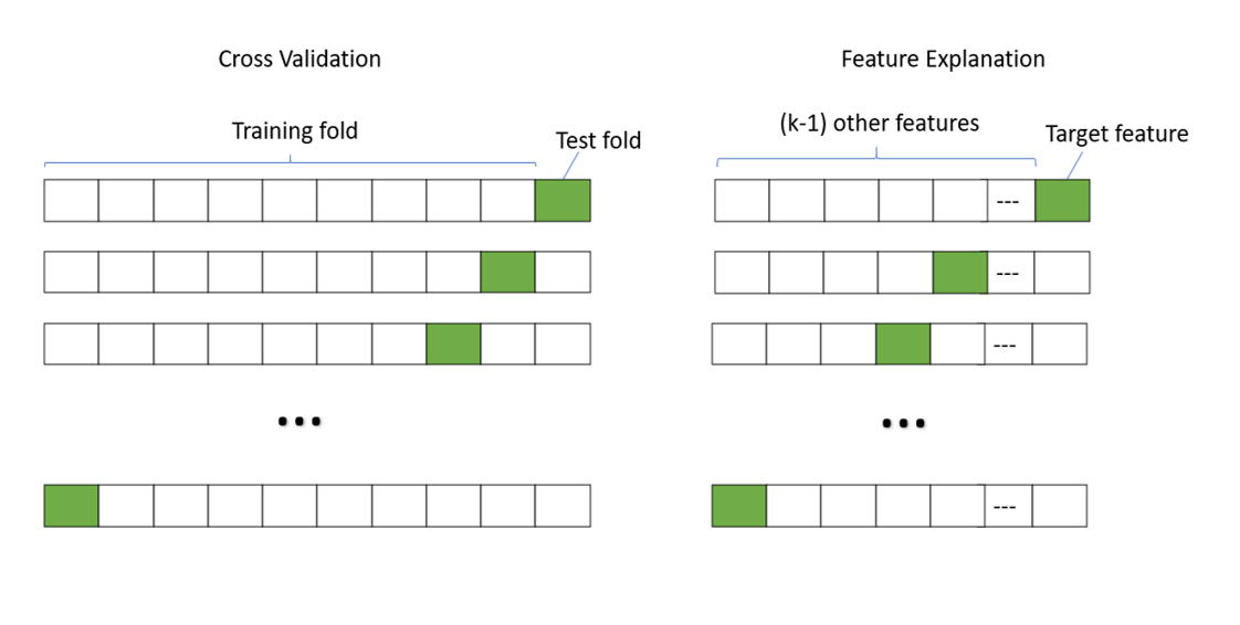
Figure 2: Comparison between cross validation and feature explanation

Experimental Study

We evaluate the performance of our feature explanation method using tree-structure models with standard data sets. In the test process, we simulate the workflow in Figure 1. Our results are evaluated by test accuracy and time efficiency according to the models we selected. We considered $k$-fold as a benchmark cross validation method compared to feature explanation method.

Experiment Subjects

“Features” are the core hyperparameter of all tree models, which means that it is important to combine ”features” with model selection and/or model interpretation in tree models. Considering characteristics of hyper-parameters in tree-structure models, we designed explanation based on feature selection for tree-structure models. Specifically, we select Decision Tree, Random Forest, Extra Trees, Gradient Boosting and XGBClassifier for simulation. Hyper-parameters used in these models are through parameter tuning (Lavesson and Davidsson 2006) with available parameters in models. To tree-structure models, important features as “max depth”, “min sample leaf” and “criterion” are included; “max features” is limited by quantity of features.

Table 1: This table shows the property of data sets used in experimental study. The #Classes, #Instances, #Features and #Attribute present the number of classes, instances, features and attribute characteristics, respectively.

	#Classes	#Instances	#Features	#Attribute
Breast Cancer	2	286	9	Real
Indian Diabetes	2	768	8	Integer, Real
Iris	3	150	4	Real
Bank loan	2	5000	10	Real
Wine	3	178	13	Integer, Real

Datasets

We list details of data sets we have used in the experiment (cf. Table 1) for both binary and multi-object classification. We choose some classification datasets encompassing different areas, complexities and data size. The standard data sets contains Breast Cancer Wisconsin Dataset (Street, Wolberg, and Mangasarian 1993), Pima Indians Diabetes Database (Smith et al. 1988), Iris Data Set (Fisher 1936), Universal Bank Loan Data Set (from Kaggle), Wine Data Set (Forina et al. 1991). The dataset will be split into training dataset and test dataset (0.7/0.3) when using feature explanation as a method. When using cross validation, we will further split 20% of training dataset for validation.

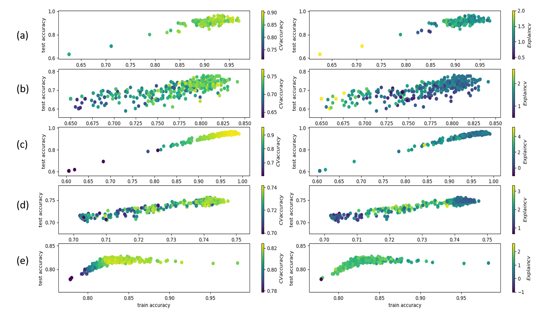
Figure 3: relationship between feature explanation and accuracy matrix for the following tasks/models: (a) Breast Cancer dataset and DecisionTree, (b) Indian Diabetes dataset and DecisionTree, (c) Spam dataset (Cranor and LaMacchia 1998) and XgboostTree, (d) Bank loan dataset and DecisionTree, (e) Credit Card dataset (Yeh and Lien 2009) and XgboostTree model.

Table 2: This table compares performance of 10-fold cross validation method (referred to as CV) and feature explanation method (FE), using test accuracy as evaluation criteria.

		DecisionTree	RandomForest	ExtraTree	GradientBoostingTree	XgboostTree
Breast Cancer	test Acc (CV/FE)	92.78% / 93.18%	96.88%/96.30%	95.13%/95.13%	96.68%/96.49%	95.03%/95.78%
	exec time (s)	19.459 / 3.288	2071 / 153	584 / 62	105 / 19	74 / 1.897
Indian Diabetes	test Acc (CV/FE)	73.30% / 72.58%	74.17%/74.75%	76.76%/75.76%	75.18%/75.04%	75.32%/75.90%
	exec time (s)	34.668 / 5.543	2200 / 174	990 / 102	237 / 33	117 / 2.194
Iris	test Acc (CV/FE)	100%/100%	100%/100%	100%/100%	100%/100%	100%/100%
	exec time (s)	3.976 / 1.666	2419 / 133	664 / 51	467 / 51	77 / 0.965
Bank loan	test Acc (CV/FE)	74.67%/74.93%	73.82%/73.78%	75.26%/75.26%	71.56%/71.56%	73.86%/73.47%
	exec time (s)	63.922 / 10.183	4393 / 959	1826 / 227	606 / 103	324 / 6.312
Wine	test Acc (CV/FE)	93.21%/93.83%	98.76%/99.38%	98.76%/100%	93.82%/92.59%	98.48%/98.41%
	exec time (s)	13.793 / 5.656	2334 / 142	558 / 56	660 / 76	114 / 1.268

Evaluation Criteria

In this research, we focus on using feature explanation in model selection. When we compare performance of cross validation based selection and model selection by feature explanation, time efficiency and accuracy (ACC) performance are two factors we consider. Similar to normal model selection process, after we trained the tree models using parameter tuning with training datasets, we will use test datasets to evaluate the accuracy performance of selecting models according to accuracy matrix.

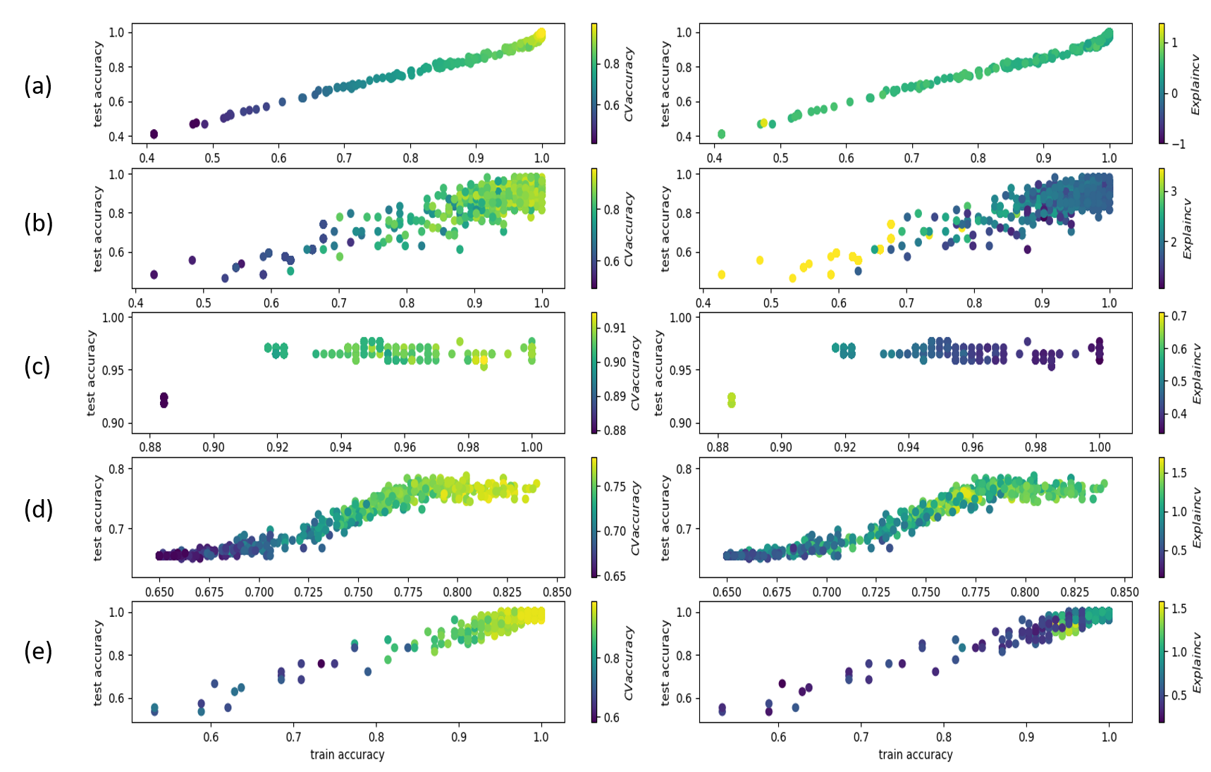
Figure 4: relationship between feature explanation and accuracy matrix for the following tasks/models: (a) Avila dataset (from UCI) and XgboostTree, (b) Wine dataset and DecisionTree, (c) Breast Cancer dataset and RandomForest, (d) Indian Diabetes dataset and DecisionTree, (e) Wine dataset and Extratree model.

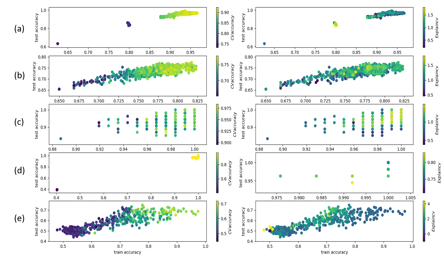
Figure 5: relationship between feature explanation and accuracy matrix for the following tasks/models: (a) Breast Cancer dataset and GradientBoostingTree, (b) Indian Diabetes dataset and GradientBoostingTree, (c) Wine dataset and GradientBoostingTree, (d) Wine dataset and RandomForest, (e) Gametes1 (from OpenML) dataset and XgboostTree model.

Research Questions

To evaluate our method and compare it to cross validation in model selection, we explore the following research questions (RQs, for short):

RQ1.

What is the relationship between feature explanation and accuracy matrix in model selection? How can we apply feature explanation method to select tree models?

We know that feature explanation evaluates tree models from training accuracy, features contribution and model complexity. We need to experimentally evaluate what is the relationship between explanation and (test) accuracy. Depending on the empirical findings about the relationship, we could apply feature explanation method in tree models selection.

RQ2.

What is the effect to apply our feature explanation method in model selection compared to $k$-fold cross validation?

Applying the results from RQ1 about selecting tree models using feature explanation, we need to experimentally compare the performance of our method with $k$-fold cross validation. The evaluation will look at accuracy performance and computational cost (time).

Experimental Results

In this section, we present the results of the experimental study, and interpret the research questions sequentially and separately to explain why the proposed approach is better than traditional cross-validation in model selection.

RQ1: Relationship between feature explanations and accuracy matrix

As discussed above, feature explanation explain tree models from training accuracy, features contribution and model complexity. When we apply feature explanation in model selection, we experiment the relationship between feature explanations and accuracy matrix using classification datasets. We have listed five of the results of relationship between feature explanations and accuracy matrix in Figure 3 from experiments of Decision tree model and Xgboost tree model. Each point in the relationship figure refers to a model evaluation based on hyperparameter tuning. In each experiment we present two figures, plotting the relationship between train accuracy and test accuracy. The experiment uses cross validation accuracy (CVaccuracy in figure) and $Explain_{cv}$ value (we defined in Eq 3) as control group. When we perform model selection, the results of cross-validation accuracy is the core evaluation to select “good” model after training the model under most cases. The left part of this figure shows that cross validation cannot always select models with higher test accuracy. The right part of figure shows that when the value of feature explanation is smaller, the model is likely to achieve a higher test accuracy. It is worth noting that the distribution of models’ test accuracy under cross validation and feature explanation is very similar. From Figure 3, cases (a) and (b) reflect cases in which it is hard to select models with best test accuracy by cross validation or feature explanation method, as shown by the sparse plots in test accuracy. The other three experiments – (c), (d), (e) – perform effectively. When the training accuracy is high and applying feature explanation method, smaller feature explanation values can lead to higher test accuracy. From the point distribution level, cross validation and feature explanation appear to aggregate when selecting models with high test accuracy, which might because cross validation and feature explanation have similar learning effects of features’ characteristics. Figure 4 and Figure 5 are provided for completeness; the plots show more results for the relationship between features and accuracy matrix. In most cases, we find that low values of feature explanation lead to higher test accuracy (which means “better” models have been found). Some cases do not have clear distinction between accuracy of cross validation and feature explanation (e.g., cases (c) and (d) in Figure 5), which might be caused by model overfitting and datasets that are too simple for the task at hand.

The results show that compared to cross validation, in the majority of cases, the value of feature explanation in tree models show an inverse relationship with test accuracy. When we have a high test accuracy, feature explanation method and normal cross validation method have dense distribution. This means, feature explanation allows to find models with high test accuracy when the model’s feature explanation value is low.

RQ2: Feature Explanation in Model Selection

To evaluate the performance of feature explanation in model selection compared to cross validation method, we simulate the basic model selection on five datasets (cf. Table 2). “Test Acc” means the average test accuracy from the best three models selected from cross validation method (CV) and feature explanation method (FE). The results show that feature explanation method could select same or better models than cross validation method. In general, half of experiments show that FE achieve higher test accuracy of best three selected models than cross validation methods. In some cases (for example cases in GradientBoostingTree), FE achieves slightly worse test accuracy (no more than 1%). “Exec time” refers to the execution time when applying CV and FE method in model selection respectively (including the whole process of model selection, cf. Figure 1). The results show that FE method saves at least 300% of execution time when selecting models in tree-structure models. Time efficiency of feature explanation is because the comparison of mechanism between CV and FE (cf. Figure 2). In model selection, the program needs to retrain and evaluate the model up to ten times (in 10-fold cross validation), which costs too much time. In feature explanation method instead, models that have been trained will be analysed by features contribution according to models’ formation and features’ contribution.

The results show that feature explanation performs at least as well as general cross validation method ($k$-fold) in tree-structure model selection while feature explanation method has a notable advantages in time efficiency. It means that we can safely replace general cross validation with feature explanation method in tree-structure model selection in the vast majority of cases.

Threats to Validity

The feature explanation method in this research is based on a novel notion in tree models (containing training accuracy, features contribution and model complexity). So this method is very sensitive to input features. Consider the noise of features (we consider the “noise” as repeated or inappropriate features in datasets); selecting bias of features in datasets might impact the practical efficacy of our method. For example, in cases in which there is no benchmark feature collections (like financial market price prediction), the same model works better on datasets including more reasonable features than datasets with unreasonable ones. It means, the application of our method might take more time on feature selection in the data processing phase.

Another threat we must point out is about the settings of hyperparemeters in models. In our experimental study, hyperparemeters are selected from a reasonable search space. But we cannot cover all possible hyperparemeters in the experiments. In this research, we select most hyperparemeters that work for classification purpose.

The stochastic characteristics of model evaluation is also a threat. We are trying to mitigate this threat by running 20 times each of the experiments and choosing 5 different tree models to increase the diversity domain of all aspects.

Conclusions

In this paper, we propose a new tree-model explanation approach for the model selection. According to our experiments, the results show that, in the vast majority of the cases, feature explanation allows to select models with high test accuracy when the model’s feature explanation value is low. Compared to general cross validation method ($k$-fold), our method performs better or similar in model selection performance while our method has a large efficiency improvement in model selection execution time. At the same time, we noticed that feature explanation based model selection would be impacted by features selection (eliminate noise generated by useless features).

Possible future research directions might be the optimization of this explanation method and its application to other machine learning models.

References

- Apley and Zhu (2016) Apley, D. W.; and Zhu, J. 2016. Visualizing the effects of predictor variables in black box supervised learning models. arXiv preprint arXiv:1612.08468 .
- Arlot, Celisse et al. (2010) Arlot, S.; Celisse, A.; et al. 2010. A survey of cross-validation procedures for model selection. Statistics surveys 4: 40–79.
- Bies et al. (2006) Bies, R. R.; Muldoon, M. F.; Pollock, B. G.; Manuck, S.; Smith, G.; and Sale, M. E. 2006. A genetic algorithm-based, hybrid machine learning approach to model selection. Journal of pharmacokinetics and pharmacodynamics 33(2): 195–221.
- Breiman (2001) Breiman, L. 2001. Random forests. Machine learning 45(1): 5–32.
- Brown (2012) Brown, C. E. 2012. Applied multivariate statistics in geohydrology and related sciences. Springer Science & Business Media.
- Cranor and LaMacchia (1998) Cranor, L. F.; and LaMacchia, B. A. 1998. Spam! Communications of the ACM 41(8): 74–83.
- Fisher, Rudin, and Dominici (2019) Fisher, A.; Rudin, C.; and Dominici, F. 2019. All Models are Wrong, but Many are Useful: Learning a Variable’s Importance by Studying an Entire Class of Prediction Models Simultaneously. Journal of Machine Learning Research 20(177): 1–81.
- Fisher (1936) Fisher, R. A. 1936. The use of multiple measurements in taxonomic problems. Annals of eugenics 7(2): 179–188.
- Forina et al. (1991) Forina, M.; Lanteri, S.; Armanino, C.; et al. 1991. Parvus-an extendible package for data exploration, classification and correlation, institute of pharmaceutical and food analysis and technologies, via brigata salerno, 16147 genoa, italy (1988). Av. Loss Av. O set Av. Hit-Rate .
- Friedman, Hastie, and Tibshirani (2001) Friedman, J.; Hastie, T.; and Tibshirani, R. 2001. The elements of statistical learning, volume 1. Springer series in statistics New York.
- Friedman (2001) Friedman, J. H. 2001. Greedy function approximation: a gradient boosting machine. Annals of statistics 1189–1232.
- Goldstein et al. (2015) Goldstein, A.; Kapelner, A.; Bleich, J.; and Pitkin, E. 2015. Peeking inside the black box: Visualizing statistical learning with plots of individual conditional expectation. Journal of Computational and Graphical Statistics 24(1): 44–65.
- Greenwell, Boehmke, and McCarthy (2018) Greenwell, B. M.; Boehmke, B. C.; and McCarthy, A. J. 2018. A simple and effective model-based variable importance measure. arXiv preprint arXiv:1805.04755 .
- Guidotti et al. (2018) Guidotti, R.; Monreale, A.; Ruggieri, S.; Turini, F.; Giannotti, F.; and Pedreschi, D. 2018. A survey of methods for explaining black box models. ACM computing surveys (CSUR) 51(5): 1–42.
- Hooker (2004) Hooker, G. 2004. Discovering additive structure in black box functions. In Proceedings of the tenth ACM SIGKDD international conference on Knowledge discovery and data mining, 575–580.
- Khalid, Khalil, and Nasreen (2014) Khalid, S.; Khalil, T.; and Nasreen, S. 2014. A survey of feature selection and feature extraction techniques in machine learning. In 2014 Science and Information Conference, 372–378. IEEE.
- Kohavi et al. (1995) Kohavi, R.; et al. 1995. A study of cross-validation and bootstrap for accuracy estimation and model selection. In Ijcai, volume 14, 1137–1145. Montreal, Canada.
- Kozak and Kozak (2003) Kozak, A.; and Kozak, R. 2003. Does cross validation provide additional information in the evaluation of regression models? Canadian Journal of Forest Research 33(6): 976–987.
- Lavesson and Davidsson (2006) Lavesson, N.; and Davidsson, P. 2006. Quantifying the impact of learning algorithm parameter tuning. In AAAI, volume 6, 395–400.
- Louppe et al. (2013) Louppe, G.; Wehenkel, L.; Sutera, A.; and Geurts, P. 2013. Understanding variable importances in forests of randomized trees. In Advances in neural information processing systems, 431–439.
- Lundberg et al. (2020) Lundberg, S. M.; Erion, G.; Chen, H.; DeGrave, A.; Prutkin, J. M.; Nair, B.; Katz, R.; Himmelfarb, J.; Bansal, N.; and Lee, S.-I. 2020. From local explanations to global understanding with explainable AI for trees. Nature machine intelligence 2(1): 2522–5839.
- McLachlan, Do, and Ambroise (2005) McLachlan, G. J.; Do, K.-A.; and Ambroise, C. 2005. Analyzing microarray gene expression data, volume 422. John Wiley & Sons.
- Molnar (2019) Molnar, C. 2019. Interpretable Machine Learning: A Guide for Making Black Box Models Explainable.(2019). URL https://christophm. github. io/interpretable-ml-book .
- Molnar (2020) Molnar, C. 2020. Interpretable Machine Learning. Lulu. com.
- Rai (2020) Rai, A. 2020. Explainable AI: From black box to glass box. Journal of the Academy of Marketing Science 48(1): 137–141.
- Raschka (2018) Raschka, S. 2018. Model evaluation, model selection, and algorithm selection in machine learning. arXiv preprint arXiv:1811.12808 .
- Rudin (2019) Rudin, C. 2019. Stop explaining black box machine learning models for high stakes decisions and use interpretable models instead. Nature Machine Intelligence 1(5): 206–215.
- Schaffer (1993) Schaffer, C. 1993. Selecting a classification method by cross-validation. Machine Learning 13(1): 135–143.
- Smith et al. (1988) Smith, J. W.; Everhart, J.; Dickson, W.; Knowler, W.; and Johannes, R. 1988. Using the ADAP learning algorithm to forecast the onset of diabetes mellitus. In Proceedings of the Annual Symposium on Computer Application in Medical Care, 261. American Medical Informatics Association.
- Street, Wolberg, and Mangasarian (1993) Street, W. N.; Wolberg, W. H.; and Mangasarian, O. L. 1993. Nuclear feature extraction for breast tumor diagnosis. In Biomedical image processing and biomedical visualization, volume 1905, 861–870. International Society for Optics and Photonics.
- Strobl et al. (2008) Strobl, C.; Boulesteix, A.-L.; Kneib, T.; Augustin, T.; and Zeileis, A. 2008. Conditional variable importance for random forests. BMC bioinformatics 9(1): 307.
- Yeh and Lien (2009) Yeh, I.-C.; and Lien, C.-h. 2009. The comparisons of data mining techniques for the predictive accuracy of probability of default of credit card clients. Expert Systems with Applications 36(2): 2473–2480.
- Zheng and Casari (2018) Zheng, A.; and Casari, A. 2018. Feature engineering for machine learning: principles and techniques for data scientists. ” O’Reilly Media, Inc.”.