A new full 3D model of cosmogenic tritium 3H production in the atmosphere (CRAC:3H)
Abstract
A new model of cosmogenic tritium (3H) production in the atmosphere is presented. The model belongs to the CRAC (Cosmic-Ray Atmospheric Cascade) family and is named as CRAC:3H. It is based on a full Monte-Carlo simulation of the cosmic-ray induced atmospheric cascade using the Geant4 toolkit. The CRAC:3H model is able, for the first time, to compute tritium production at any location and time, for any given energy spectrum of the primary incident cosmic ray particles, explicitly treating, also for the first time, particles heavier than protons. This model provides a useful tool for the use of 3H as a tracer of atmospheric and hydrological circulation. A numerical recipe for practical use of the model is appended.
JGR: Atmospheres
Sodankylä Geophysical Observatory, University of Oulu, Finland Space Physics and Astronomy Research Unit, University of Oulu, Finland Ioffe Physical-Technical Institute, St. Petersburg, Russia
Stepan Poluianovstepan.poluianov@oulu.fi
A new CRAC:3H model of cosmogenic tritium (3H) production in the atmosphere is presented.
For the first time, it provides 3D production, also explicitly treating particles heavier than protons.
This model provides a useful tool for the use of 3H as a tracer of atmospheric and hydrological circulation.
1 Introduction
Tritium (3H) is a radioactive isotope of hydrogen with the half-life time of approximately 12.3 years. As an isotope of hydrogen, it is involved in the global water cycle and forms a very useful tracer of atmospheric moisture (e.g., Sykora \BBA Froehlich, \APACyear2010; Juhlke \BOthers., \APACyear2020) or hydrological cycles (Michel, \APACyear2005). In the natural environment, tritium is mostly produced by galactic cosmic rays (GCR) in the atmosphere, as a sub-product of the induced nucleonic cascade, and is thus a cosmogenic radionuclide. On the other hand, tritium is also produced artificially in thermonuclear bomb tests. Before the nuclear-test ban became in force, a huge amount of tritium had been produced artificially and realised into the atmosphere, leading to an increase of the global reservoir inventory of tritium by two orders of magnitude above the natural level (e.g., Sykora \BBA Froehlich, \APACyear2010; Cauquoin \BOthers., \APACyear2016). Thus, the cosmogenic production of tritium was typically neglected as being too small against anthropogenic one. However, as nearly 60 years have passed since the nuclear tests, its global content has reduced to the natural pre-bomb level (Palcsu \BOthers., \APACyear2018) and presently is mostly defined by the cosmogenic production. Accordingly, natural variability of the isotope production can be again used in atmospheric tracing, water vapour transport, dynamics of the stratosphere-troposphere exchanges over Antarctica (Cauquoin \BOthers., \APACyear2015; Fourré \BOthers., \APACyear2018; Palcsu \BOthers., \APACyear2018; Juhlke \BOthers., \APACyear2020; László \BOthers., \APACyear2020). Moreover, a combination of the 3H data with other tracers like atmospheric 10Be, which is also produced by cosmic-ray spallation reactions, but whose transport is different, can be a very powerful research tool. For this purpose, a reliable production model is needed, which is able to provide a full 3D and time variable production of tritium in the atmosphere.
Some models of tritium production by cosmic rays (CR) in the atmosphere were developed earlier. First models (Fireman, \APACyear1953; Craig \BBA Lal, \APACyear1961; Nir \BOthers., \APACyear1966; Lal \BBA Peters, \APACyear1967; O’Brien, \APACyear1979) were based on simplified numerical or semi-empirical methods of modelling the cosmic-ray induced atmospheric cascade. Later, a full Monte-Carlo simulation of the cosmogenic isotope production in the atmospheric cascade had been developed (Masarik \BBA Beer, \APACyear1999) leading to higher accuracy of the results. However, that model had some significant limitations: (1) were considered only GCR protons (heavier GCR species were treated as scaled protons); (2) the energy spectrum of GCR was prescribed; (3) only global and latitudinal zonal mean productions were presented, implying no spatial resolution. That model was slightly revisited by Masarik \BBA Beer (\APACyear2009), but the methodological approach remained the same. A more recent tritium production model developed by Webber \BOthers. (\APACyear2007) is also based on a full Monte-Carlo simulation of the atmospheric cascade and was built upon the yield-function approach which allows dealing with any kind of the cosmic-ray spectrum. However, only columnar (for the entire atmospheric column) production was provided by those authors, making it impossible to model the height distribution of isotope production. Moreover, that model was dealing with CR protons only, while the contribution of heavier species to cosmogenic isotope production can be as large as 40% (see section 3).
Here we present a new model of cosmogenic tritium production in the atmosphere, that is based on a full simulation of the cosmic-ray induced atmospheric cascade. This model belongs to the CRAC (Cosmic-Ray Atmospheric Cascade) family and is named as CRAC:3H. The CRAC:3H model is able, for the first time, to compute tritium production at any location and time, for any given energy spectrum of the primary incident CR particles, explicitly treating, also for the first time, particles heavier than protons. This model provides a useful tool for the use of 3H as a tracer of atmospheric and hydrological circulation.
2 Production model
The local production rate of a cosmogenic isotope, in atoms per second per gram of air, at a given location with the geomagnetic rigidity cutoff and the atmospheric depth can be written as
| (1) |
where is the intensity of incident cosmic-ray particles of the -th type (characterized by the charge and atomic mass numbers) in units of particles per (s sr cm2 GeV), is the isotope yield function in units of (atoms sr cm2 g-1, — see section 2.1 for details), is the kinetic energy of the incident particle in GeV, is the atmospheric depth in units of (g/cm2), is the energy corresponding to the local geomagnetic cutoff rigidity for a particle of type , and the summation is over the particle types. GeV is the proton’s rest mass. The geomagnetic rigidity cutoff quantifies the shielding effect of the geomagnetic field and can be roughly interpreted as a rigidity/energy threshold of primary incident charged particles required to imping on the atmosphere (see formalism in Elsasser, \APACyear1956; Smart \BOthers., \APACyear2000).
2.1 Production function
Here we computed the tritium production function in a way similar to our previous works in the framework of the CRAC-family models (e.g., Usoskin \BBA Kovaltsov, \APACyear2008; Kovaltsov \BBA Usoskin, \APACyear2010; Kovaltsov \BOthers., \APACyear2012; Poluianov \BOthers., \APACyear2016), viz. by applying a full Monte-Carlo simulation of the cosmic-ray induced atmospheric cascade, as briefly described below. Full description of the nomenclature and numerical approach is available in Poluianov \BOthers. (\APACyear2016).
The yield function (see equation 1) of a nuclide of interest provides the number of atoms produced in the unit (1 g/cm2) atmospheric layer by incident particles of type (e.g., cosmic ray protons, -particles, heavier species) with the fixed energy and the unit intensity (1 particle per cm2 per steradian). The yield function should not be confused with the so-called production function , which is defined as the number of nuclide atoms produced in the unit atmospheric layer per one incident particle with the energy . In a case of the isotropic particle distribution, these quantities are related as
| (2) |
where is the conversion factor between the particle intensity in space and the particle flux at the top of the atmosphere (see, e.g., chapter 1.6.2 in Grieder, \APACyear2001).
The production function in units (atoms cm2/g) can be calculated, for the isotropic flux of primary CR particles of type , as
| (3) |
where summation is over types of secondary particles of the cascade (can be protons, neutrons, -particles), is the ‘aggregate’ cross-section (see below) in units (cm2/g), and are concentration and velocity of the secondary particles of type with energy at depth . The aggregate cross-section is defined as
| (4) |
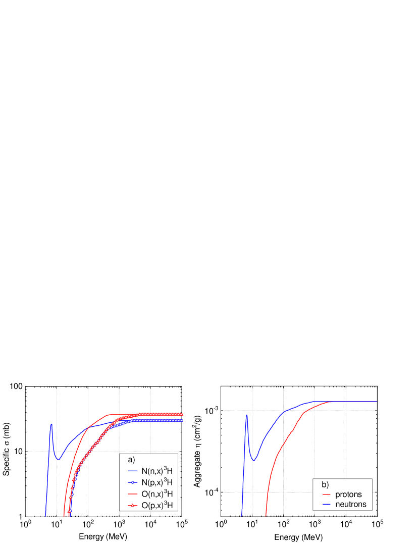
where indicates the type of a target nucleus in the air (nitrogen and oxygen for tritium), is the number of the target nuclei of type in one gram of air, is the total cross-section of nuclear reactions between the -th atmospheric cascade particle and the -th target nucleus yielding the nuclide of interest. Atmospheric tritium is produced by spallation of target nuclei of nitrogen and oxygen, which have the values of g-1 and g-1, respectively. The reactions yielding tritium are caused mainly by the cascade neutrons and protons and include: N(n,x)3H; N(p,x)3H; O(n,x)3H; O(p,x)3H. The cross-sections used here were adopted from Nir \BOthers. (\APACyear1966) and Coste \BOthers. (\APACyear2012), as shown in Figure 1a. We assumed that cross-sections of the neutron-induced reactions are similar to those for protons above the energy of 2 GeV. For reactions caused by -particles, N(,x)3H and O(,x)3H, the cross-sections were assessed from proton ones according to Tatischeff \BOthers. (\APACyear2006). These reactions are induced mostly by -particles from the primary CRs and are, hence, important only in the upper atmospheric layers.
The tritium aggregate cross-sections (equation 4) are shown in Figure 1b. Although production efficiencies of protons and neutrons are similar at high energies, they differ significantly in the 500 MeV range. Because of the lower energy threshold and higher cross-sections for neutrons in this energy range, comparing to protons, tritium production is dominated by neutrons in a region where the cascade is fully-developed, viz., in the lower part of the atmosphere.
The quantity describing the cascade particles (equation 3) was computed using a full Monte Carlo simulation of the cascade induced in the atmosphere by energetic cosmic-ray particles. The general computation scheme was similar to that applied by Poluianov \BOthers. (\APACyear2016). The simulation code was based on the Geant4 toolkit v.10.0 (Agostinelli \BOthers., \APACyear2003; Allison \BOthers., \APACyear2006). In particular, we used the physics list QGSP_BIC_HP (Quark-Gluon String model for high-energy interactions; Geant4 Binary Cascade model; High-Precision neutron package) (Geant4 collaboration, \APACyear2013), which was shown to describe the cosmic ray cascade with sufficient accuracy (e.g., Mesick \BOthers., \APACyear2018). We simulated a real-scale spherical atmosphere with the inner radius of 6371 km, height of 100 km and thickness of 1050 g/cm2. The atmosphere was divided into homogeneous spherical layers with the thickness ranging from 1 g/cm2 (at the top) to 10 g/cm2 near the ground. The atmospheric composition and density profiles were taken according to the atmospheric model NRLMSISE-00 (Picone \BOthers., \APACyear2002). Cosmic rays were simulated as isotropic fluxes of mono-energetic protons and -particles, while heavier species were considered as scaled particles (see section 2.2). The simulations were performed with a logarithmic grid of energies between 20 MeV/nuc and 100 GeV/nuc. The number of simulated incident particles was set so that the statistical accuracy of the isotope production should be better than 1% in any location. This number varied from 1000 incident particles for particles with the energy of 100 GeV/nucleon to simulations for 20-MeV protons. The results were extrapolated to higher energies, up to 1000 GeV/nuc, by applying a power law. The yield of the secondary particles (protons, neutrons and -particles) at the top of each atmospheric layer was recorded as histograms with the spectral (logarithmic) resolution of 20 bins per one order of magnitude in the range of the secondary particle’s energy between 1 keV and 100 GeV. The primary CR particles were also recorded in the same way.
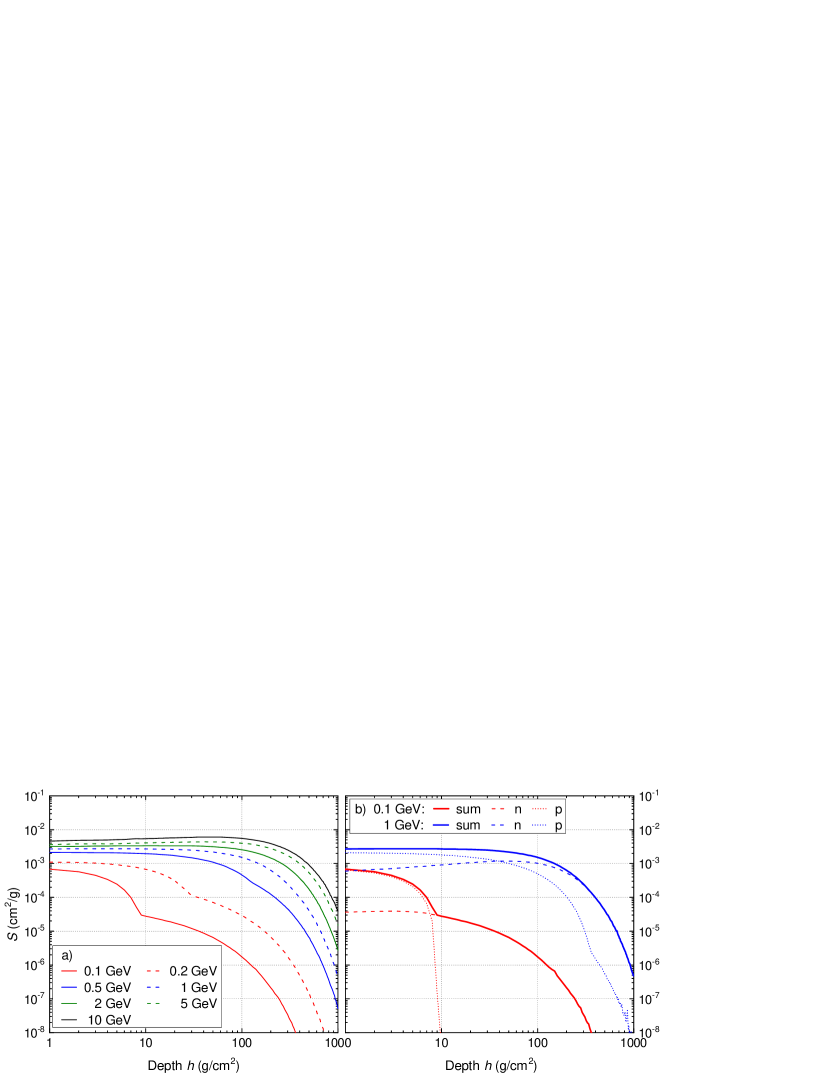
The production functions were subsequently calculated from the simulation results, using equation (3), for a prescribed grid of energies and atmospheric depths and are tabulated in the Supporting Information. Some examples of the tritium production function are shown in Figure 2 for primary CR protons. One can see in Figure 2a that the efficiency of tritium atom production grows with the energy of the incident particles because of larger atmospheric cascades induced. Contributions of different components to the total production are shown in Figure 2b for low (0.1 GeV) and medium (1 GeV) energies of the primary proton. The red curve for the 0.1 GeV incident protons depicts a double-bump structure: the bump in the upper atmospheric layers (10 g/cm2) is caused by spallation reactions caused mostly by the primary protons (as indicated by the red dotted curve), while the smooth curve at higher depths is due to secondary neutrons (red dashed curve). Overall, production of tritium at depths greater than 10 g/cm2 is very small for the low-energy primary protons. On the other hand, higher-energy (1 GeV, blue curves in Figure 2b) protons effectively form a cascade reaching the ground, where the contribution of secondary neutrons dominates below g/cm2 depths.
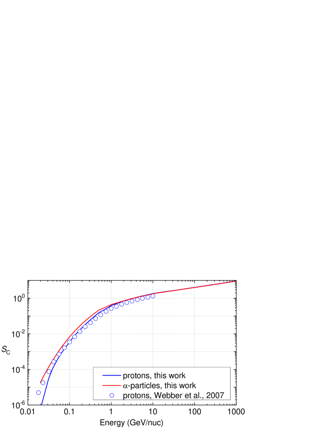
This type of the depth/altitude profiles or the tritium production function was not studied in earlier works, where only columnar functions, viz. integrated over the full atmospheric column, were presented (Webber \BOthers., \APACyear2007). Therefore, in order to compare our results with the earlier published ones, we also calculated the columnar production function
| (5) |
where g/cm2 is the atmospheric depth at the mean sea level or the thickness of the entire atmospheric column. The columnar production function is tabulated in the Supporting Information and depicted in Figure 3 along with the earlier results published by Webber \BOthers. (\APACyear2007) for incident protons. No results for incident -particles have been published earlier, and the production function of cosmogenic tritium by cosmic-ray -particles is presented here for the first time. One can see that, while the production functions for incident protons generally agree between our work and the results by Webber \BOthers. (\APACyear2007), there are some small but systematic differences. In particular, our result is lower than that of Webber \BOthers. (\APACyear2007) in the low-energy range below 100 MeV. It should be noted that the contribution of this energy region to the total production of tritium is negligible because of the geomagnetic shielding in such a way that low-energy incident particles can impinge on the atmosphere only in spatially small polar regions. In the energy range above 200 MeV, the tritium production function computed here is higher than that from Webber \BOthers. (\APACyear2007). The difference is not large, %, but systematic and can be related to the uncertainties in the cross-sections or details of the cascade simulation (FLUKA vs. Geant4). Overall, our model predicts slightly higher production of tritium than the one by Webber \BOthers. (\APACyear2007), for the same cosmic-ray flux.
2.2 Cosmic-ray spectrum
The first term in equation (1) refers to the spectrum of differential intensity of the incident cosmic-ray particles. A standard way to model the GCR spectrum for practical applications is based on the so-called force-field approximation (Gleeson \BBA Axford, \APACyear1967; Caballero-Lopez \BBA Moraal, \APACyear2004; Usoskin \BOthers., \APACyear2005), which parameterizes the spectrum with reasonable accuracy even during disturbed periods, as validated by direct in-space measurements (Usoskin \BOthers., \APACyear2015). In this approximation, the differential energy spectrum of the -th component of GCR near Earth (outside of the Earth’s magnetosphere and atmosphere) is parameterized in the following form:
| (6) |
where is the differential intensity of GCR particles in the local interstellar medium, often called the local interstellar spectrum (LIS), is the particle’s kinetic energy per nucleon, is the rest energy of a proton (0.938 GeV), and is the modulation parameter defined by the modulation potential as well as the charge () and atomic () numbers of the particle of type , respectively. The spectrum at any moment of time is fully determined by a single time-variable parameter , which has the dimension of potential (typically given in MV or GV) and is called the modulation potential. The absolute value of makes no physical sense and depends on the exact shape of LIS (see discussion in Usoskin \BOthers., \APACyear2005; Herbst \BOthers., \APACyear2010, \APACyear2017; Asvestari \BOthers., \APACyear2017).
In this work, we made use of a recent parameterization of the proton LIS (Vos \BBA Potgieter, \APACyear2015), which is partly based on direct in situ measurements of GCR:
| (7) |
where is the differential intensity of GCR protons in the local interstellar medium in units of particles per (s sr cm2 GeV), and are the particle’s kinetic energy (in GeV) and the velocity-to-speed-of-light ratio, respectively. Following a recent work (Koldobskiy \BOthers., \APACyear2019) based on a joint analysis of data from the space-borne experiment AMS-02 (Alpha Magnetic Spectrometer) and from the ground-based neutron-monitor network, we assumed that LIS (in the number of nucleons) of all heavier (2) GCR species can be represented by the LIS for protons scaled with a factor of 0.353 for the same energy per nucleon.
The integral production rate in the entire atmospheric column is called the columnar production rate. For a given location, characterized by the geomagnetic cutoff rigidity , and at the time moment it is defined as
| (8) |
The global production rate is the spatial average of over the globe, while the integral of over the globe yields the total production of tritium.
Production of tritium by GCR, which always bombard the Earth’s atmosphere, is described above. Production by solar energetic particles (SEP) can be computed in a similar way, with the SEP energy spectrum entering directly in equation (1).
3 Results
Using the production function computed here (section 2.1) and applying equations (1) and (8), we calculated the mean production rate of tritium in the atmosphere for different levels of solar modulation (low, moderate and high), for the entire atmosphere and only for the troposphere. The results are shown in Table 1. The modeled local production rates (equation 1) used for the computation can be found in a tabular form in the supporting information.
| Solar activity | Entire atm. | Troposphere | ||
|---|---|---|---|---|
| Global | Polar | Global | Polar | |
| Low | 0.41 | 0.92 | 0.12 | 0.16 |
| Moderate | 0.345 | 0.72 | 0.11 | 0.14 |
| High | 0.27 | 0.51 | 0.09 | 0.10 |
The global production rate of tritium for a moderate solar activity ( MV), which is the mean level for the modern epoch (Usoskin \BOthers., \APACyear2017), is 0.345 atoms/(s cm2). This value can be compared with earlier estimates of the global production rate of tritium. We performed a literature survey and found that the estimates performed before 1999 were based on different approximated approaches and vary by a factor of 2.5, between 0.14–0.36 atoms/(s cm2) (Craig \BBA Lal, \APACyear1961; Nir \BOthers., \APACyear1966; O’Brien, \APACyear1979; Masarik \BBA Reedy, \APACyear1995). Modern estimates, based on full Monte-Carlo simulations, are more constrained. The early value of the global production rate of 0.28 atoms/(s cm2) published by Masarik \BBA Beer (\APACyear1999) was revised by the authors to 0.32 atoms/(s cm2) in Masarik \BBA Beer (\APACyear2009). Our value is very close to that, despite the different computational schemes and assumptions made. The computed global production rate also agrees with the estimates obtained from reservoir inventories (e.g. Craig \BBA Lal, \APACyear1961), that are, however, loosely constrained within a factor of about four, between 0.2–0.8 atoms/(s cm2). We note that heavier-than-proton primary incident particles contribute about 40% to the global production of tritium, in the case of GCR, and thus, it is very important to consider these particles explicitly.
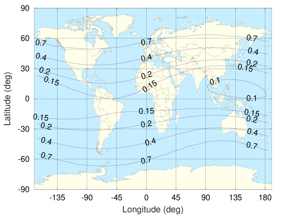
Geographical distribution of the columnar production rate of tritium is shown in Figure 4. It is defined primarily by the geomagnetic cutoff rigidity (e.g., Smart \BBA Shea, \APACyear2009; Nevalainen \BOthers., \APACyear2013) and varies by an order of magnitude between the high-cutoff spot in the equatorial west-Pacific region and polar regions.
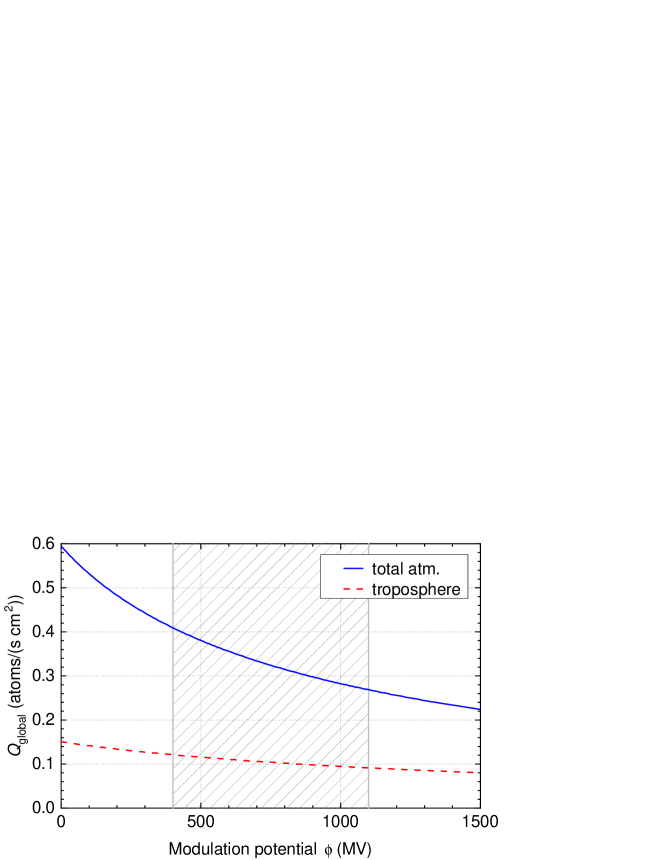
Dependence of the global production rate of tritium on solar activity quantified via the modulation potential is shown in Figure 5, both for the entire atmosphere and for the troposphere. The tropospheric contribution to the global production is about 31% on average, ranging from 30% (solar minimum) to 34% (solar maximum).
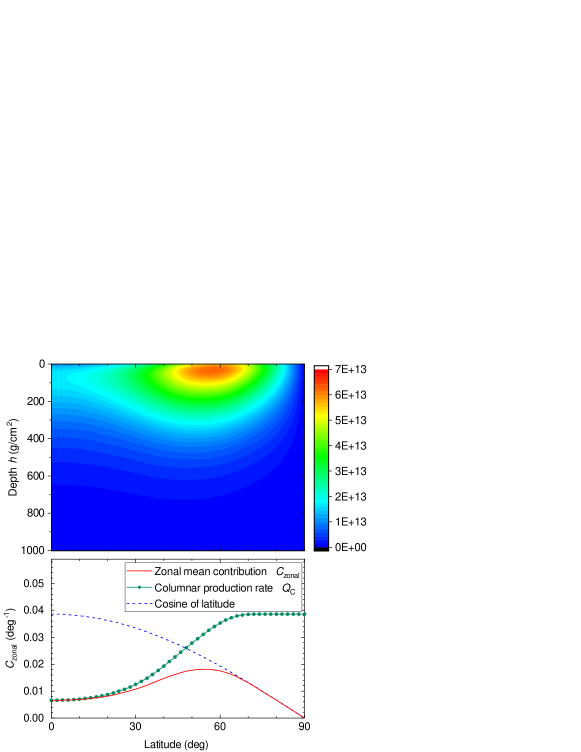
Even though the production rate is significantly higher in the polar region, its contribution to the global production is not dominant, because of the small area of the polar regions. Figure 6 (upper panel) presents the production rate of tritium in latitudinal zones (integrated over longitude in one degree of geographical latitude) as a function of geographical latitude and atmospheric depth. It has a broad maximum at mid-latitudes (40–70∘) in the stratosphere (10–100 g/cm2 of depth) and ceases both towards the poles and ground. The bottom panel of the Figure depicts the zonal mean contribution (red curve) of the entire atmospheric column into the total global production. It illustrates that the distribution with a maximum at mid-latitudes shape is defined by two concurrent processes: the enhanced production (green curve) and reduced zonal area (blue curve) from the equator to the pole. The zonal contribution is proportional to the product of these two processes.
The altitude profile of the tritium production rate by GCR for the moderate level of solar activity is shown in Figure 7. The maximum of the globally averaged production is located at about 40 g/cm2 or 20 km of altitude in the stratosphere, corresponding to the Regener-Pfotzer maximum where the atmospheric cascade is most developed. The maximum of production is somewhat higher in the polar region because of the reduced geomagnetic shielding there, so that lower-energy CR particles can reach the location.
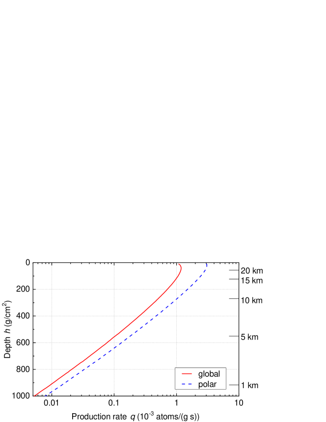
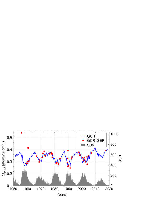
Figure 8 depicts temporal variability of the global tritium production for the period 1951–2018, computed using the model presented here. To indicate the solar cycle shape, the sunspot numbers are also shown in the bottom. The contribution from GCR is shown by the blue curve and computed using the modulation potential reconstructed from the neutron-monitor network (Usoskin \BOthers., \APACyear2017). Red dots consider also additional production of tritium by strong SEP events, identified as ground-level enhancement (GLE) events (http://gle.oulu.fi). This is negligible on the long run but may contribute essentially on the short-time scale. Overall, the production of tritium is mostly driven by the heliospheric modulation of GCR as implied by obvious anti-correlation with the sunspot numbers.
4 Conclusion
A new full model CRAC:3H of tritium cosmogenic production in the atmosphere is presented. It is able to compute the tritium production rate at any location in 3D and for any type of the incident particle energy spectrum/intensity — slowly variable galactic cosmic rays or intense sporadic events of solar energetic particles. The core of the model is the yield/production function, rigorously computed by applying a full Monte-Carlo simulation of the cosmic-ray induced atmospheric cascade with high statistics and is tabulated in the Supporting Information. Using this tabulated function, one can straightforwardly and easily calculate the production of tritium for any conditions in the Earth’s atmosphere (see Appendix A), including solar modulation of GCR, sporadic SEP events, changes of the geomagnetic field, etc. The columnar and global production of tritium, computed by the new model, is comparable with most recent estimates by other groups, but is significantly higher than the results of earlier models, published before 2000. It also agrees well with empirical estimates of the tritium reservoir inventories, considering large uncertainties of the latter. Thus, for the first time, a reliable model is developed that provides a full 3D production of tritium in the atmosphere. These results can be used as an input for atmospheric transport models or for direct comparison with tritium observations that are important for the study of solar activity in link with the hydrological cycle or for evaluation of the atmospheric dynamics in models.
Appendix A Calculation of tritium production: Numerical algorithm
Using the production function presented here in the Supporting Information, one can easily compute tritium production at any given location (quantified by the local geomagnetic rigidity cutoff and atmospheric depth ), and time , following the numerical algorithm below.
-
1.
For a given moment of time , the intensity of incident primary particles can be evaluated, in case of GCR, using equations (6) and (7) for the independently known modulation potential (e.g., as provided at http://cosmicrays.oulu.fi/phi/phi.html). These formulas can be directly applied for protons, while the contribution of heavier species (2) can be considered, using the same formulas, but applying the scaling factor of 0.353 for LIS, which is given in number of nucleons, and considering kinetic energy per nucleon. Thus, the input intensities of the incident protons and heavier species , the latter effectively including all heavier species, can be obtained. Energy should be in units of GeV, and in units of nucleons per (sr cm2 s GeV). The energy grid is recommended to be logarithmic (at least 10 points per order of magnitude).
-
2.
The production function for the given atmospheric depth can be obtained, for both protons and heavier species , from the Supporting Information in units of (cm2/g). The yield function is defined as , in units of (sr cm2/g), also separately for protons and heavier species. The product of the yield function and the intensity of incident particles is called the response function , separately for protons and heavier species.
-
3.
As the next step, the local geomagnetic rigidity cutoff , which is related to the lower integration bound in equation (1), needs to be calculated for a given location and time. A good balance between simplicity and realism is provided by the eccentric tilted dipole approximation of the geomagnetic field (Nevalainen \BOthers., \APACyear2013). The value of in this approximation can be computed using a detailed numerical recipe (Appendix A in Usoskin \BOthers., \APACyear2010). This approach works well with GCR, but is too rough for an analysis of SEP events, where a detailed computations of the geomagnetic shielding is needed (e.g., Mishev \BOthers., \APACyear2014).
-
4.
Next, the response function should be integrated above the energy bound defined by the geomagnetic rigidity cutoff , as specified in equation (1) separately for the protons and particles (the latter effectively includes also heavier 2 species). Since the response function is very sharp, the use of standard methods of numerical integration, such as trapezoids, Gauss, etc., may lead to large uncertainties. For numerical integration of equation (1), the piecewise power-law approximation is recommended, as described below. Let function whose values are defined at grid points and as and , respectively, be approximated by a power law between these grid points. Then its integral on the interval between these grid points is
(9) The final production rate at the given location, atmospheric depth and time is the sum of the two components (protons and particles).
-
5.
In a case when not only the very local production rate of tritium is required, but spatially integrated or averaged, the columnar production function (equation 8) can be used. The spatially averaged/integrated production can be then obtained by averaging/integration over the appropriate area considering the changes in the geomagnetic cutoff rigidity .
Acknowledgements.
The yield/production functions of tritium, obtained in this work, are available in the Supporting Information to this paper. The used cross-section data can be found in Nir \BOthers. (\APACyear1966) and Coste \BOthers. (\APACyear2012). The toolkit Geant4 (Agostinelli \BOthers., \APACyear2003; Allison \BOthers., \APACyear2006) is freely distributed under Geant4 Software License at http://www.geant4.org. This work used publicly available data for SEP events from the GLE database (http://gle.oulu.fi), sunspot number series from SILSO (http://www.sidc.be/silso/datafiles, Clette \BBA Lefèvre, \APACyear2016), heliospheric modulation potential series provided by the Oulu cosmic ray station (http://cosmicrays.oulu.fi/phi/phi.html). S.P. acknowledges the International Joint Research Program of ISEE, Nagoya University, and thanks Naoyuki Kurita from Nagoya University for valuable discussion. This work was partly supported by the Academy of Finland (Projects ESPERA no. 321882 and ReSoLVE Centre of Excellence, no. 307411).References
- Agostinelli \BOthers. (\APACyear2003) \APACinsertmetastarGeant4-1{APACrefauthors}Agostinelli, S., Allison, J., Amako, K., Apostolakis, J., Araujo, H., Arce, P.\BDBLZschiesche, D. \APACrefYearMonthDay2003. \BBOQ\APACrefatitleGeant4 - a simulation toolkit Geant4 - a simulation toolkit.\BBCQ \APACjournalVolNumPagesNucl. Instr. Meth. Phys. A5063250–303. {APACrefURL} http://www.sciencedirect.com/science/article/pii/S0168900203013688 {APACrefDOI} http://dx.doi.org/10.1016/S0168-9002(03)01368-8 \PrintBackRefs\CurrentBib
- Allison \BOthers. (\APACyear2006) \APACinsertmetastarGeant4-2{APACrefauthors}Allison, J., Amako, K., Apostolakis, J., Araujo, H., Dubois, P., Asai, M.\BDBLYoshida, H. \APACrefYearMonthDay2006. \BBOQ\APACrefatitleGeant4 developments and applications Geant4 developments and applications.\BBCQ \APACjournalVolNumPagesNuclear Science, IEEE Transactions on531270-278. {APACrefDOI} 10.1109/TNS.2006.869826 \PrintBackRefs\CurrentBib
- Asvestari \BOthers. (\APACyear2017) \APACinsertmetastarAsvestari_JGR2017{APACrefauthors}Asvestari, E., Gil, A., Kovaltsov, G.\BCBL \BBA Usoskin, I. \APACrefYearMonthDay2017. \BBOQ\APACrefatitleNeutron Monitors and Cosmogenic Isotopes as Cosmic Ray Energy-Integration Detectors: Effective Yield Functions, Effective Energy, and Its Dependence on the Local Interstellar Spectrum Neutron Monitors and Cosmogenic Isotopes as Cosmic Ray Energy-Integration Detectors: Effective Yield Functions, Effective Energy, and Its Dependence on the Local Interstellar Spectrum.\BBCQ \APACjournalVolNumPagesJ. Geophys. Res. Space Phys.122109790-9802. {APACrefDOI} 10.1002/2017JA024469 \PrintBackRefs\CurrentBib
- Caballero-Lopez \BBA Moraal (\APACyear2004) \APACinsertmetastarCaballero-Lopez_JGR2004{APACrefauthors}Caballero-Lopez, R\BPBIA.\BCBT \BBA Moraal, H. \APACrefYearMonthDay2004. \BBOQ\APACrefatitleLimitations of the force field equation to describe cosmic ray modulation Limitations of the force field equation to describe cosmic ray modulation.\BBCQ \APACjournalVolNumPagesJ. Geophys. Res.: Space Phys.109A1A01101. {APACrefURL} http://dx.doi.org/10.1029/2003JA010098 {APACrefDOI} 10.1029/2003JA010098 \PrintBackRefs\CurrentBib
- Cauquoin \BOthers. (\APACyear2016) \APACinsertmetastarcauguoin16{APACrefauthors}Cauquoin, A., Jean-Baptiste, P., Risi, C., Fourré, É.\BCBL \BBA Landais, A. \APACrefYearMonthDay2016. \BBOQ\APACrefatitleModeling the global bomb tritium transient signal with the AGCM LMDZ-iso: A method to evaluate aspects of the hydrological cycle Modeling the global bomb tritium transient signal with the AGCM LMDZ-iso: A method to evaluate aspects of the hydrological cycle.\BBCQ \APACjournalVolNumPagesJ. Geophys. Res. (Atmos.)1212112,612-12,629. {APACrefDOI} 10.1002/2016JD025484 \PrintBackRefs\CurrentBib
- Cauquoin \BOthers. (\APACyear2015) \APACinsertmetastarcauquoin15{APACrefauthors}Cauquoin, A., Jean-Baptiste, P., Risi, C., Fourré, É., Stenni, B.\BCBL \BBA Landais, A. \APACrefYearMonthDay2015. \BBOQ\APACrefatitleThe global distribution of natural tritium in precipitation simulated with an Atmospheric General Circulation Model and comparison with observations The global distribution of natural tritium in precipitation simulated with an Atmospheric General Circulation Model and comparison with observations.\BBCQ \APACjournalVolNumPagesEarth Planet. Sci. Lett.427160-170. {APACrefDOI} 10.1016/j.epsl.2015.06.043 \PrintBackRefs\CurrentBib
- Clette \BBA Lefèvre (\APACyear2016) \APACinsertmetastarclette16{APACrefauthors}Clette, F.\BCBT \BBA Lefèvre, L. \APACrefYearMonthDay2016. \BBOQ\APACrefatitleThe New Sunspot Number: Assembling All Corrections The New Sunspot Number: Assembling All Corrections.\BBCQ \APACjournalVolNumPagesSolar Phys.2912629-2651. {APACrefDOI} 10.1007/s11207-016-1014-y \PrintBackRefs\CurrentBib
- Coste \BOthers. (\APACyear2012) \APACinsertmetastarCoste_AnA2012{APACrefauthors}Coste, B., Derome, L., Maurin, D.\BCBL \BBA Putze, A. \APACrefYearMonthDay2012. \BBOQ\APACrefatitleConstraining Galactic cosmic-ray parameters with nuclei Constraining galactic cosmic-ray parameters with nuclei.\BBCQ \APACjournalVolNumPagesAstron. Astrophys.539A88. {APACrefURL} https://doi.org/10.1051/0004-6361/201117927 {APACrefDOI} 10.1051/0004-6361/201117927 \PrintBackRefs\CurrentBib
- Craig \BBA Lal (\APACyear1961) \APACinsertmetastarcraig61{APACrefauthors}Craig, H.\BCBT \BBA Lal, D. \APACrefYearMonthDay1961. \BBOQ\APACrefatitleThe Production Rate of Natural Tritium The Production Rate of Natural Tritium.\BBCQ \APACjournalVolNumPagesTellus Ser. A13185-105. {APACrefDOI} 10.1111/j.2153-3490.1961.tb00068.x \PrintBackRefs\CurrentBib
- Elsasser (\APACyear1956) \APACinsertmetastarElsasser_N1956{APACrefauthors}Elsasser, W. \APACrefYearMonthDay1956. \BBOQ\APACrefatitleCosmic-Ray Intensity and Geomagnetism Cosmic-Ray Intensity and Geomagnetism.\BBCQ \APACjournalVolNumPagesNature1781226-1227. {APACrefDOI} 10.1038/1781226a0 \PrintBackRefs\CurrentBib
- Fireman (\APACyear1953) \APACinsertmetastarfireman53{APACrefauthors}Fireman, E\BPBIL. \APACrefYearMonthDay1953. \BBOQ\APACrefatitleMeasurement of the (n, H3) Cross Section in Nitrogen and Its Relationship to the Tritium Production in the Atmosphere Measurement of the (n, H3) Cross Section in Nitrogen and Its Relationship to the Tritium Production in the Atmosphere.\BBCQ \APACjournalVolNumPagesPhys. Rev.914922-926. {APACrefDOI} 10.1103/PhysRev.91.922 \PrintBackRefs\CurrentBib
- Fourré \BOthers. (\APACyear2018) \APACinsertmetastarfourre18{APACrefauthors}Fourré, E., Landais, A., Cauquoin, A., Jean-Baptiste, P., Lipenkov, V.\BCBL \BBA Petit, J\BPBIR. \APACrefYearMonthDay2018. \BBOQ\APACrefatitleTritium Records to Trace Stratospheric Moisture Inputs in Antarctica Tritium Records to Trace Stratospheric Moisture Inputs in Antarctica.\BBCQ \APACjournalVolNumPagesJ. Geophys. Res. (Atmos.)12363009-3018. {APACrefDOI} 10.1002/2018JD028304 \PrintBackRefs\CurrentBib
- Geant4 collaboration (\APACyear2013) \APACinsertmetastarGeant4-Phys2013{APACrefauthors}Geant4 collaboration. \APACrefYearMonthDay2013. \BBOQ\APACrefatitlePhysics reference manual (version geant4 9.10.0) Physics reference manual (version geant4 9.10.0)\BBCQ [\bibcomputersoftwaremanual]. \APACrefnoteavailable from http://geant4.cern.ch/support/index.shtml \PrintBackRefs\CurrentBib
- Gleeson \BBA Axford (\APACyear1967) \APACinsertmetastarGleeson_ApJ1967{APACrefauthors}Gleeson, J\BPBIJ.\BCBT \BBA Axford, W\BPBII. \APACrefYearMonthDay1967. \BBOQ\APACrefatitleCosmic rays in the interplanetary medium Cosmic rays in the interplanetary medium.\BBCQ \APACjournalVolNumPagesAstrophys. J.149L115. {APACrefURL} http://adsabs.harvard.edu/abs/1967ApJ...149L.115G {APACrefDOI} 10.1086/180070 \PrintBackRefs\CurrentBib
- Grieder (\APACyear2001) \APACinsertmetastarGrieder2001{APACrefauthors}Grieder, P\BPBIK\BPBIF. \APACrefYear2001. \APACrefbtitleCosmic Rays at Earth Cosmic Rays at Earth. \APACaddressPublisherAmsterdamElsevier Science. \PrintBackRefs\CurrentBib
- Herbst \BOthers. (\APACyear2010) \APACinsertmetastarHerbst_JGR2010{APACrefauthors}Herbst, K., Kopp, A., Heber, B., Steinhilber, F., Fichtner, H., Scherer, K.\BCBL \BBA Matthiä, D. \APACrefYearMonthDay2010. \BBOQ\APACrefatitleOn the importance of the local interstellar spectrum for the solar modulation parameter On the importance of the local interstellar spectrum for the solar modulation parameter.\BBCQ \APACjournalVolNumPagesJ. Geophys. Res.: Atmos.115D1D00I20. {APACrefURL} http://dx.doi.org/10.1029/2009JD012557 {APACrefDOI} 10.1029/2009JD012557 \PrintBackRefs\CurrentBib
- Herbst \BOthers. (\APACyear2017) \APACinsertmetastarHerbst_JGR2017{APACrefauthors}Herbst, K., Muscheler, R.\BCBL \BBA Heber, B. \APACrefYearMonthDay2017. \BBOQ\APACrefatitleThe new local interstellar spectra and their influence on the production rates of the cosmogenic radionuclides 10Be and 14C The new local interstellar spectra and their influence on the production rates of the cosmogenic radionuclides 10Be and 14C.\BBCQ \APACjournalVolNumPagesJournal of Geophysical Research: Space Physics122123-34. {APACrefDOI} 10.1002/2016JA023207 \PrintBackRefs\CurrentBib
- Juhlke \BOthers. (\APACyear2020) \APACinsertmetastarjuhlke20{APACrefauthors}Juhlke, T., Sültenfuß, J., Trachte, K., Huneau, F., Garel, E., Santoni, S.\BDBLvan Geldern, R. \APACrefYearMonthDay2020. \BBOQ\APACrefatitleTritium as a hydrological tracer in Mediterranean precipitation events Tritium as a hydrological tracer in Mediterranean precipitation events.\BBCQ \APACjournalVolNumPagesAtmos. Chem. Phys.2063555-3568. {APACrefDOI} 10.5194/acp-20-3555-2020 \PrintBackRefs\CurrentBib
- Koldobskiy \BOthers. (\APACyear2019) \APACinsertmetastarKoldobskiy_JGR2019{APACrefauthors}Koldobskiy, S\BPBIA., Bindi, V., Corti, C., Kovaltsov, G\BPBIA.\BCBL \BBA Usoskin, I\BPBIG. \APACrefYearMonthDay2019. \BBOQ\APACrefatitleValidation of the Neutron Monitor Yield Function Using Data From AMS-02 Experiment, 2011-2017 Validation of the Neutron Monitor Yield Function Using Data From AMS-02 Experiment, 2011-2017.\BBCQ \APACjournalVolNumPagesJ. Geophys. Res.: Space Phys.12442367-2379. {APACrefDOI} 10.1029/2018JA026340 \PrintBackRefs\CurrentBib
- Kovaltsov \BOthers. (\APACyear2012) \APACinsertmetastarKovaltsov_EPSL2012{APACrefauthors}Kovaltsov, G\BPBIA., Mishev, A.\BCBL \BBA Usoskin, I\BPBIG. \APACrefYearMonthDay2012. \BBOQ\APACrefatitleA new model of cosmogenic production of radiocarbon 14C in the atmosphere A new model of cosmogenic production of radiocarbon 14C in the atmosphere.\BBCQ \APACjournalVolNumPagesEarth Planet. Sci. Lett.337114-120. {APACrefDOI} 10.1016/j.epsl.2012.05.036 \PrintBackRefs\CurrentBib
- Kovaltsov \BBA Usoskin (\APACyear2010) \APACinsertmetastarKovaltsov_EPSL2010{APACrefauthors}Kovaltsov, G\BPBIA.\BCBT \BBA Usoskin, I\BPBIG. \APACrefYearMonthDay2010. \BBOQ\APACrefatitleA new 3D numerical model of cosmogenic nuclide 10Be production in the atmosphere A new 3D numerical model of cosmogenic nuclide 10Be production in the atmosphere.\BBCQ \APACjournalVolNumPagesEarth Planet. Sci. Lett.291182-188. {APACrefDOI} 10.1016/j.epsl.2010.01.011 \PrintBackRefs\CurrentBib
- Lal \BBA Peters (\APACyear1967) \APACinsertmetastarlal67{APACrefauthors}Lal, D.\BCBT \BBA Peters, B. \APACrefYearMonthDay1967. \BBOQ\APACrefatitleCosmic Ray Produced Radioactivity on the Earth Cosmic ray produced radioactivity on the earth.\BBCQ \BIn K. Sittle (\BED), \APACrefbtitleHandbuch der Physik Handbuch der physik (\BVOL 46, \BPGS 551–612). \APACaddressPublisherBerlinSpringer. \PrintBackRefs\CurrentBib
- László \BOthers. (\APACyear2020) \APACinsertmetastarlaszlo20{APACrefauthors}László, E., Palcsu, M.\BCBL \BBA Leelőssy, Á. \APACrefYearMonthDay2020. \BBOQ\APACrefatitleEstimation of the solar-induced natural variability of the tritium concentration of precipitation in the Northern and Southern Hemisphere Estimation of the solar-induced natural variability of the tritium concentration of precipitation in the Northern and Southern Hemisphere.\BBCQ \APACjournalVolNumPagesAtmos. Envir.. {APACrefDOI} 10.1016/j.atmosenv.2020.117605 \PrintBackRefs\CurrentBib
- Masarik \BBA Beer (\APACyear1999) \APACinsertmetastarMasarik_JGR1999{APACrefauthors}Masarik, J.\BCBT \BBA Beer, J. \APACrefYearMonthDay1999. \BBOQ\APACrefatitleSimulation of particle fluxes and cosmogenic nuclide production in the Earth’s atmosphere Simulation of particle fluxes and cosmogenic nuclide production in the Earth’s atmosphere.\BBCQ \APACjournalVolNumPagesJ. Geophys. Res.10412099-12112. {APACrefDOI} 10.1029/1998JD200091 \PrintBackRefs\CurrentBib
- Masarik \BBA Beer (\APACyear2009) \APACinsertmetastarMasarik_JGR2009{APACrefauthors}Masarik, J.\BCBT \BBA Beer, J. \APACrefYearMonthDay2009. \BBOQ\APACrefatitleAn updated simulation of particle fluxes and cosmogenic nuclide production in the Earth’s atmosphere An updated simulation of particle fluxes and cosmogenic nuclide production in the Earth’s atmosphere.\BBCQ \APACjournalVolNumPagesJ. Geophys. Res.114D11103. {APACrefDOI} 10.1029/2008JD010557 \PrintBackRefs\CurrentBib
- Masarik \BBA Reedy (\APACyear1995) \APACinsertmetastarmasarik95{APACrefauthors}Masarik, J.\BCBT \BBA Reedy, R\BPBIC. \APACrefYearMonthDay1995. \BBOQ\APACrefatitleTerrestrial cosmogenic-nuclide production systematics calculated from numerical simulations Terrestrial cosmogenic-nuclide production systematics calculated from numerical simulations.\BBCQ \APACjournalVolNumPagesEarth Planet. Sci. Lett.136381-395. {APACrefDOI} 10.1016/0012-821X(95)00169-D \PrintBackRefs\CurrentBib
- Mesick \BOthers. (\APACyear2018) \APACinsertmetastarmesick18{APACrefauthors}Mesick, K\BPBIE., Feldman, W\BPBIC., Coupland, D\BPBID\BPBIS.\BCBL \BBA Stonehill, L\BPBIC. \APACrefYearMonthDay2018. \BBOQ\APACrefatitleBenchmarking Geant4 for Simulating Galactic Cosmic Ray Interactions Within Planetary Bodies Benchmarking Geant4 for Simulating Galactic Cosmic Ray Interactions Within Planetary Bodies.\BBCQ \APACjournalVolNumPagesEarth Space Sci.57324-338. {APACrefDOI} 10.1029/2018EA000400 \PrintBackRefs\CurrentBib
- Michel (\APACyear2005) \APACinsertmetastarmichel05{APACrefauthors}Michel, R. \APACrefYearMonthDay2005. \BBOQ\APACrefatitleTritium in the hydrological cycle Tritium in the hydrological cycle.\BBCQ \BIn P. Aggarwal, J. Gat\BCBL \BBA K. Froehlich (\BEDS), \APACrefbtitleIsotopes in the Water Cycle. Past, Present and Future of a Developing Science Isotopes in the Water Cycle. Past, Present and Future of a Developing Science (\BPG 53-66). \APACaddressPublisherDordtrechtSpringer. \PrintBackRefs\CurrentBib
- Mishev \BOthers. (\APACyear2014) \APACinsertmetastarMishev2014{APACrefauthors}Mishev, A\BPBIL., Kocharov, L\BPBIG.\BCBL \BBA Usoskin, I\BPBIG. \APACrefYearMonthDay2014. \BBOQ\APACrefatitleAnalysis of the ground level enhancement on 17 May 2012 using data from the global neutron monitor network Analysis of the ground level enhancement on 17 may 2012 using data from the global neutron monitor network.\BBCQ \APACjournalVolNumPagesJ. Geophys. Res.: Space Phys.1192670–679. {APACrefURL} http://dx.doi.org/10.1002/2013JA019253 {APACrefDOI} 10.1002/2013JA019253 \PrintBackRefs\CurrentBib
- Nevalainen \BOthers. (\APACyear2013) \APACinsertmetastarNevalainen2013{APACrefauthors}Nevalainen, J., Usoskin, I.\BCBL \BBA Mishev, A. \APACrefYearMonthDay2013. \BBOQ\APACrefatitleEccentric dipole approximation of the geomagnetic field: Application to cosmic ray computations Eccentric dipole approximation of the geomagnetic field: Application to cosmic ray computations.\BBCQ \APACjournalVolNumPagesAdv. Space Res.52122-29. {APACrefDOI} http://dx.doi.org/10.1016/j.asr.2013.02.020 \PrintBackRefs\CurrentBib
- Nir \BOthers. (\APACyear1966) \APACinsertmetastarNir_RGSP1966{APACrefauthors}Nir, A., Kruger, S\BPBIT., Lingenfelter, R\BPBIE.\BCBL \BBA Flamm, E\BPBIJ. \APACrefYearMonthDay1966. \BBOQ\APACrefatitleNatural Tritium Natural Tritium.\BBCQ \APACjournalVolNumPagesRev. Geophys. Space Phys.4441-456. {APACrefDOI} 10.1029/RG004i004p00441 \PrintBackRefs\CurrentBib
- O’Brien (\APACyear1979) \APACinsertmetastarOBrien_JGR1979{APACrefauthors}O’Brien, K. \APACrefYearMonthDay1979. \BBOQ\APACrefatitleSecular variations in the production of cosmogenic isotopes in the earth’s atmosphere Secular variations in the production of cosmogenic isotopes in the earth’s atmosphere.\BBCQ \APACjournalVolNumPagesJ. Geophys. Res.84423-431. {APACrefDOI} 10.1029/JA084iA02p00423 \PrintBackRefs\CurrentBib
- Palcsu \BOthers. (\APACyear2018) \APACinsertmetastarpalcsu18{APACrefauthors}Palcsu, L., Morgenstern, U., Sültenfuss, J., Koltai, G., László, E., Temovski, M.\BDBLJull, A\BPBIJ. \APACrefYearMonthDay2018. \BBOQ\APACrefatitleModulation of Cosmogenic Tritium in Meteoric Precipitation by the 11-year Cycle of Solar Magnetic Field Activity Modulation of Cosmogenic Tritium in Meteoric Precipitation by the 11-year Cycle of Solar Magnetic Field Activity.\BBCQ \APACjournalVolNumPagesSci. Rep.812813. {APACrefDOI} 10.1038/s41598-018-31208-9 \PrintBackRefs\CurrentBib
- Picone \BOthers. (\APACyear2002) \APACinsertmetastarPicone2002{APACrefauthors}Picone, J\BPBIM., Hedin, A\BPBIE., Drob, D\BPBIP.\BCBL \BBA Aikin, A\BPBIC. \APACrefYearMonthDay2002. \BBOQ\APACrefatitleNRLMSISE-00 empirical model of the atmosphere: Statistical comparisons and scientific issues Nrlmsise-00 empirical model of the atmosphere: Statistical comparisons and scientific issues.\BBCQ \APACjournalVolNumPagesJ. Geophys. Res.: Space Phys.107A12SIA 15-1–SIA 15-16. {APACrefURL} http://dx.doi.org/10.1029/2002JA009430 \APACrefnote1468 {APACrefDOI} 10.1029/2002JA009430 \PrintBackRefs\CurrentBib
- Poluianov \BOthers. (\APACyear2016) \APACinsertmetastarPoluianov_JGR2016{APACrefauthors}Poluianov, S\BPBIV., Kovaltsov, G\BPBIA., Mishev, A\BPBIL.\BCBL \BBA Usoskin, I\BPBIG. \APACrefYearMonthDay2016. \BBOQ\APACrefatitleProduction of cosmogenic isotopes 7Be, 10Be, 14C, 22Na, and 36Cl in the atmosphere: Altitudinal profiles of yield functions Production of cosmogenic isotopes 7Be, 10Be, 14C, 22Na, and 36Cl in the atmosphere: Altitudinal profiles of yield functions.\BBCQ \APACjournalVolNumPagesJournal of Geophysical Research (Atmospheres)1218125-8136. {APACrefDOI} 10.1002/2016JD025034 \PrintBackRefs\CurrentBib
- Raukunen \BOthers. (\APACyear2018) \APACinsertmetastarRaukunen_SWSC2018{APACrefauthors}Raukunen, O., Vainio, R., Tylka, A\BPBIJ., Dietrich, W\BPBIF., Jiggens, P., Heynderickx, D.\BDBLSiipola, R. \APACrefYearMonthDay2018. \BBOQ\APACrefatitleTwo solar proton fluence models based on ground level enhancement observations Two solar proton fluence models based on ground level enhancement observations.\BBCQ \APACjournalVolNumPagesJournal of Space Weather and Space Climate827A04. {APACrefDOI} 10.1051/swsc/2017031 \PrintBackRefs\CurrentBib
- Smart \BBA Shea (\APACyear2009) \APACinsertmetastarSmart2009{APACrefauthors}Smart, D.\BCBT \BBA Shea, M. \APACrefYearMonthDay2009. \BBOQ\APACrefatitleFifty years of progress in geomagnetic cutoff rigidity determinations Fifty years of progress in geomagnetic cutoff rigidity determinations.\BBCQ \APACjournalVolNumPagesAdv. Space Res.44101107–1123. {APACrefURL} http://www.sciencedirect.com/science/article/pii/S0273117709004815 {APACrefDOI} http://dx.doi.org/10.1016/j.asr.2009.07.005 \PrintBackRefs\CurrentBib
- Smart \BOthers. (\APACyear2000) \APACinsertmetastarshea00{APACrefauthors}Smart, D\BPBIF., Shea, M\BPBIA.\BCBL \BBA Flückiger, E\BPBIO. \APACrefYearMonthDay2000. \BBOQ\APACrefatitleMagnetospheric Models and Trajectory Computations Magnetospheric Models and Trajectory Computations.\BBCQ \APACjournalVolNumPagesSpace Sci. Rev.93305-333. {APACrefDOI} 10.1023/A:1026556831199 \PrintBackRefs\CurrentBib
- Sykora \BBA Froehlich (\APACyear2010) \APACinsertmetastarfroehlich10{APACrefauthors}Sykora, I.\BCBT \BBA Froehlich, K. \APACrefYearMonthDay2010. \BBOQ\APACrefatitleRadionuclides as Tracers of Atmospheric Processes Radionuclides as Tracers of Atmospheric Processes.\BBCQ \BIn K. Froehlich (\BED), \APACrefbtitleEnvironmental Radionuclides: Tracers and Timers of Terrestrial Processes Environmental Radionuclides: Tracers and Timers of Terrestrial Processes (\BVOL 16, \BPG 51-88). \APACaddressPublisherAmsterdamElevier. \PrintBackRefs\CurrentBib
- Tatischeff \BOthers. (\APACyear2006) \APACinsertmetastarTatischeff_APJS2006{APACrefauthors}Tatischeff, V., Kozlovsky, B., Kiener, J.\BCBL \BBA Murphy, R\BPBIJ. \APACrefYearMonthDay2006. \BBOQ\APACrefatitleDelayed X- and Gamma-Ray Line Emission from Solar Flare Radioactivity Delayed X- and Gamma-Ray Line Emission from Solar Flare Radioactivity.\BBCQ \APACjournalVolNumPagesAstrophys. J. Suppl.165606-617. {APACrefDOI} 10.1086/505112 \PrintBackRefs\CurrentBib
- Thébault \BOthers. (\APACyear2015) \APACinsertmetastarThebault_EPS2015{APACrefauthors}Thébault, E., Finlay, C\BPBIC., Beggan, C\BPBID., Alken, P., Aubert, J., Barrois, O.\BDBLZvereva, T. \APACrefYearMonthDay2015. \BBOQ\APACrefatitleInternational Geomagnetic Reference Field: the 12th generation International Geomagnetic Reference Field: the 12th generation.\BBCQ \APACjournalVolNumPagesEarth Planet. Space6779. {APACrefDOI} 10.1186/s40623-015-0228-9 \PrintBackRefs\CurrentBib
- Usoskin \BOthers. (\APACyear2005) \APACinsertmetastarUsoskin_phi_05{APACrefauthors}Usoskin, I\BPBIG., Alanko-Huotari, K., Kovaltsov, G\BPBIA.\BCBL \BBA Mursula, K. \APACrefYearMonthDay2005. \BBOQ\APACrefatitleHeliospheric modulation of cosmic rays: Monthly reconstruction for 1951–2004 Heliospheric modulation of cosmic rays: Monthly reconstruction for 1951–2004.\BBCQ \APACjournalVolNumPagesJ. Geophys. Res.110A12108. {APACrefDOI} 10.1029/2005JA011250 \PrintBackRefs\CurrentBib
- Usoskin \BOthers. (\APACyear2017) \APACinsertmetastarUsoskin_JGR2017{APACrefauthors}Usoskin, I\BPBIG., Gil, A., Kovaltsov, G\BPBIA., Mishev, A\BPBIL.\BCBL \BBA Mikhailov, V\BPBIV. \APACrefYearMonthDay2017. \BBOQ\APACrefatitleHeliospheric modulation of cosmic rays during the neutron monitor era: Calibration using PAMELA data for 2006-2010 Heliospheric modulation of cosmic rays during the neutron monitor era: Calibration using PAMELA data for 2006-2010.\BBCQ \APACjournalVolNumPagesJ. Geophys. Res.1223875-3887. {APACrefDOI} 10.1002/2016JA023819 \PrintBackRefs\CurrentBib
- Usoskin \BBA Kovaltsov (\APACyear2008) \APACinsertmetastarUsoskin_JGR2008{APACrefauthors}Usoskin, I\BPBIG.\BCBT \BBA Kovaltsov, G\BPBIA. \APACrefYearMonthDay2008. \BBOQ\APACrefatitleProduction of cosmogenic 7Be isotope in the atmosphere: Full 3-D modeling Production of cosmogenic 7Be isotope in the atmosphere: Full 3-D modeling.\BBCQ \APACjournalVolNumPagesJ. Geophys. Res.113D12D12107. {APACrefDOI} 10.1029/2007JD009725 \PrintBackRefs\CurrentBib
- Usoskin \BOthers. (\APACyear2015) \APACinsertmetastarusoskin_PAMELA_15{APACrefauthors}Usoskin, I\BPBIG., Kovaltsov, G\BPBIA., Adriani, O., Barbarino, G\BPBIC., Bazilevskaya, G\BPBIA., Bellotti, R.\BDBLZverev, V\BPBIG. \APACrefYearMonthDay2015. \BBOQ\APACrefatitleForce-field parameterization of the galactic cosmic ray spectrum: Validation for Forbush decreases Force-field parameterization of the galactic cosmic ray spectrum: Validation for Forbush decreases.\BBCQ \APACjournalVolNumPagesAdv. Space Res.552940-2945. {APACrefDOI} 10.1016/j.asr.2015.03.009 \PrintBackRefs\CurrentBib
- Usoskin \BOthers. (\APACyear2010) \APACinsertmetastarUsoskin_JASTP2010{APACrefauthors}Usoskin, I\BPBIG., Mironova, I\BPBIA., Korte, M.\BCBL \BBA Kovaltsov, G\BPBIA. \APACrefYearMonthDay2010. \BBOQ\APACrefatitleRegional millennial trend in the cosmic ray induced ionization of the troposphere Regional millennial trend in the cosmic ray induced ionization of the troposphere.\BBCQ \APACjournalVolNumPagesJ. Atmos. Solar-Terrestr. Phys.7219-25. {APACrefDOI} 10.1016/j.jastp.2009.10.003 \PrintBackRefs\CurrentBib
- Vos \BBA Potgieter (\APACyear2015) \APACinsertmetastarVos_ApJ2015{APACrefauthors}Vos, E\BPBIE.\BCBT \BBA Potgieter, M\BPBIS. \APACrefYearMonthDay2015. \BBOQ\APACrefatitleNew Modeling of Galactic Proton Modulation during the Minimum of Solar Cycle 23/24 New Modeling of Galactic Proton Modulation during the Minimum of Solar Cycle 23/24.\BBCQ \APACjournalVolNumPagesAstrophys. J.815119. {APACrefDOI} 10.1088/0004-637X/815/2/119 \PrintBackRefs\CurrentBib
- Webber \BOthers. (\APACyear2007) \APACinsertmetastarWebber_JGR2007{APACrefauthors}Webber, W\BPBIR., Higbie, P\BPBIR.\BCBL \BBA McCracken, K\BPBIG. \APACrefYearMonthDay2007. \BBOQ\APACrefatitleProduction of the cosmogenic isotopes 3H, 7Be, 10Be, and 36Cl in the Earth’s atmosphere by solar and galactic cosmic rays Production of the cosmogenic isotopes 3H, 7Be, 10Be, and 36Cl in the Earth’s atmosphere by solar and galactic cosmic rays.\BBCQ \APACjournalVolNumPagesJournal of Geophysical Research (Space Physics)112A11A10106. {APACrefDOI} 10.1029/2007JA012499 \PrintBackRefs\CurrentBib
- Wilcox \BOthers. (\APACyear2012) \APACinsertmetastarWilcox_QJRMS2012{APACrefauthors}Wilcox, L\BPBIJ., Hoskins, B\BPBIJ.\BCBL \BBA Shine, K\BPBIP. \APACrefYearMonthDay2012. \BBOQ\APACrefatitleA global blended tropopause based on ERA data. Part I: Climatology A global blended tropopause based on ERA data. Part I: Climatology.\BBCQ \APACjournalVolNumPagesQ. J. R. Meteorol. Soc.138664561-575. {APACrefDOI} 10.1002/qj.951 \PrintBackRefs\CurrentBib