A non-linear mathematical model for the X-ray variability classes of the microquasar GRS 1915+105 - I: quiescent, spiking states and QPOs

Abstract

The microquasar GRS 1915+105 is known to exhibit a very variable X-ray emission on different time scales and patterns. We propose a system of two ordinary differential equations, adapted from the Hindmarsh-Rose model, with two dynamical variables $x(t)$, $y(t)$ and an input constant parameter $J_{0}$, to which we added a random white noise, whose solutions for the $x(t)$ variable reproduce consistently the X-ray light curves of several variability classes as well as the development of low frequency Quasi-Periodic Oscillations (QPO). We show that changing only the value of $J_{0}$ the system moves from stable to unstable solutions and the resulting light curves reproduce those of the quiescent classes like $\phi$ and $\chi$, the $\delta$ class and the spiking $\rho$ class. Moreover, we found that increasing the values of $J_{0}$ the system induces high frequency oscillations that evolve to QPO when it moves into another stable region. This system of differential equations gives then a unified view of the variability of GRS 1915+105 in term of transitions between stable and unstable states driven by a single input function $J_{0}$. We also present the results of a stability analysis of the equilibrium points and some considerations on the existence of periodic solutions.

1 Introduction

GRS 1915+105, the first microquasar, discovered by Castro-Tirado et al. (1992) is known to exhibit a large number of variability patterns on different time scales. On long time scales, months to years, changes of the X-ray flux up to about one order of magnitude are reported (Huppenkothen et al., 2017) and on time scales of thousands of seconds, light curves present either quiescent states, with red noise power spectra, or series of fast bursts. A first classification of light curves was performed by Belloni et al. (2000) who defined 12 variability classes on the basis of the spectral and timing properties of a large collection of multiepoch observations. New classes were discovered in the subsequent years (Klein-Wolt et al., 2002; Hannikainen et al., 2003, 2005) indicating that GRS 1915+105 is potentially able to develop physical conditions from which new classes of light curves can be originated. A useful compilation of light curves for about all classes can be found in Polyakov et al. (2012), and a more complete description of the rich phenomenology of this unique source is given in the review paper by Fender & Belloni (2004).

The complex hydrodynamical, thermal and magnetic phenomena occurring in accretion discs around black holes involve non-linear processes whose evolution can be described by a system of differential equations. These can be solved by numerical calculations involving several quantities not directly observable, as the gas density or viscous stresses. The stability of disc structures is also a very interesting subject of investigations since many years and theoretical analysis suggested that thermal and viscous instabilities can develop and establish a limit cycle behaviour. In particular the possibility of observing a bursting behaviour originated by thermal relaxtion oscillations between standard and slim disc states was first suggested by Honma et al. (1991) and after by Chen & Taam (1993); Szuszkiewicz & Miller (1998), before the discovery of this behaviour in GRS 1915+105. Complexity of hydrodynamic and thermodynamic equations, however, does not allow a rather simple picture of the roles played by the involved physical quantities and the interpretation of data is not simple. Moreover, the limit cycle is often described in terms of disc quantities, such as the surface density or the mass accretion rate, which are not directly observable. As stated by Fender & Belloni (2004) in their review paper “it will not be possible to interpret in detail every aspect of the complex light curves …, yet the structure is not random and contains information about the accretion disc of GRS 1915+105.”

It has been noticed that the nearly regular burst sequences of GRS 1915+105 have some similarities with signals from living systems and, in fact, it is frequently referred in the literature as the ‘hearthbeat’ state (Neilsen et al., 2011). There are many mathematical tools developed for describing similar behaviours and particularly those for the bursting of neurons. This analogy suggested us to search if some of these models could be applied in the case of GRS 1915+105 and in a couple of previous papers (Massaro et al., 2014; Ardito et al., 2017) we studied the solutions of a non-autonomous and non-linear system of two ordinary differential equations (ODE), whose solutions are able to reproduce the light curves of some variability classes. More precisely, in those two papers we considered the ODE system introduced by FitzHugh (1961) and Nagumo & Yoshizawa (1962) to model the quiescent and spiking behaviours of the classes $\phi$, $\chi$ and $\rho$. In the present paper, we propose another system of two ODEs, based on that developed by Hindmarsh & Rose (1984), which is able to reproduce light curves of several variability classes that must be considered as a useful analytical approximation for describing the evolution of instabilities and the transitions between different equilibrium states. Our goal is to clear up the most relevant features of the observed behaviours with the low complexity of the mathematical model: it will be possible to show that some dynamical regimes, like quiescent or bursting activity, are indeed obtained using a low-dimensional system of ODEs. Moreover, we will show that non-linear processes provide a unified view of other interesting phenomena as the development of low frequency Quasi-Periodic Oscillations (QPO) in accretion discs.

Non-linear oscillators were already considered in a seminal paper by Moore & Spiegel (1966) in a stellar physics context for describing the convective energy transfer. Later, Usher & Whitney (1968) and Buchler & Regev (1981) applied non linear processes to the physics of pulsating variable stars (see also Regev & Buchler, 1981; Buchler, 1993).

Researches on the instabilities in accretion discs started in the seventies (e.g. Lightman & Eardley, 1974; Pringle et al., 1973; Shakura & Sunyaev, 1976) and up to now a large number of papers was produced. Taam & Lin (1984), in particular, using numerical integration of the non-linear disc equations and applying the $\alpha$ prescription for the viscosity (Shakura & Sunyaev, 1973), investigated a thermal-viscous instability and obtained a few theoretical light curves having recurrent spikes. After the discovery of the $\rho$ class variability in GRS 1915+105, Taam et al. (1997) analysed the time and spectral properties of the bursts and proposed an interpretation based on the instability discussed in the previous paper. The evolution of thermal viscous instabilities in an accretion disc is associated with a limit cycle (e.g. Szuszkiewicz & Miller, 1998), generally described by means of S-shaped equilibrium curves in a plot of temperature or accretion rate vs disc surface density, where the different signs of the slope correspond to stable and unstable equilibrium states (e.g. Abramowicz et al., 1995). Examples are the models developed by Watarai & Mineshige (2001) (see also Mineshige & Watarai, 2005) for a slim-disc (Abramowicz et al., 1988) as indicated by the energy spectral results for GRS 1915+105 of Vierdayanti et al. (2010) and Mineo et al. (2012), and by Janiuk et al. (2000, 2002), who included dissipation processes due to the presence of a corona and an outflow. More recently Potter & Balbus (2017) demonstrated that a similar profile is found for a thermal-viscous instability induced by a turbulent accretion disc stress factor depending upon the magnetic Prandl number.

It is interesting that the topology of one of the equilibrium curves of the proposed ODE system presents a S-shaped pattern similar to those derived from numerical solutions of instability disc equations. We will show that this allows for both stable and unstable equilibrium states which provide a useful and accurate modelling of the observed X-ray light curves, including many details. In this first paper, we limit our analysis to the case of a steady input function, while the solutions for a variable input and the extension to other classes will be discussed in the companion paper Massaro et al. (2020, hereafter Paper II), together with a tentative interpretation of the equations on the basis of literature disc instability calculations.

2 The MHR non-linear ODE system

To reproduce the rich and complex behaviour of GRS 1915+105, we considered a non-linear system of ODE as those used for describing quiescent and bursting signals in neuronal arrays. This approach offers the possibility of describing transitions between stable and unstable equilibrium states with the onset of limit cycles. Mathematical aspects of this important topic were deeply investigated in the past half century and an extremely wide and technical literature is available (see, for instance the textbooks of Izhikevich 2006 or Gerstner et al. 2014).

The general formulation of the Hindmarsh-Rose (hereafter HR) system considers three ODE for the dynamical variables $x$, $y$ and $z$, involving changes on different time scales; it is generally written as:

$$\frac{dx}{dt} = \frac{1}{A}[P_{3}(x)+b_{1}y-z]$$

$$\frac{dy}{dt} = P_{2}(x)-b_{2}y$$ (1)

$$\frac{dz}{dt} = \varepsilon[s(x-x_{0})-z]$$

where $A$ is a scale factor and $P_{2}(x)$ and $P_{3}(x)$ are two polynomials of second and third degree, respectively:

$$P_{3}(x) = -a_{1}x^{3}+a_{2}x^{2}+a_{3}x+a_{4}$$

$$P_{2}(x) = -a_{5}x^{2}+a_{6}x+a_{7}$$ (2)

With the parameters’ values $A=1$, $a_{1}=1$, $a_{2}=3$, $a_{3}=a_{6}=0$, $a_{4}=5.0$, $a_{5}=5$, $a_{7}=-3$, and $b_{1}=b_{2}=1$, Eqs. 2 and 2 give the classic HR model (Hindmarsh & Rose 1984; Hindmarsh & Cornelius 2005 and the tutorial paper by Shilnikov & Kolomiets 2008). In our work we adopted a modified system of the HR equations and substituted the variable $z$ with an external input function of the time $J(t)$. The system includes, therefore, only two equations that, adopting a notation similar to that already used in Massaro et al. (2014), are written as:

$$\frac{dx}{dt} = -\rho x^{3}+\beta_{1}x^{2}+y+J(t)$$

$$\frac{dy}{dt} = -\beta_{2}x^{2}-y$$ (3)

where we indicate the two variables with $x$ and $y$, as before, and the signs of the various terms were taken to have the parameters’ values positive.

This ODE system can be easily written in a single equation in the two variables:

$$\frac{dx}{dt}=-\rho x^{3}-(\beta_{1}/\beta_{2})\frac{dy}{dt}+(1-\beta_{1}/\beta_{2})y+J(t)$$ (4)

or the equivalent one:

$$\frac{dx}{dt}=-\rho x^{3}+(\beta_{1}-\beta_{2})x^{2}-\frac{dy}{dt}+J(t)$$ (5)

that makes clear the role of the variable $y$ and its derivative in the evolution of $x$ and that when the cubic term turns to be the dominant one it would be responsible of the fast decrease just after the maximum.

In our calculations the solutions for the $x$ variable correspond to those for the X-ray luminosity, where there is the largest energy release, while the $y$ plays the role of a state variable of the disc plasma directly related to the radiative energy dissipation. Moreover, the latter quantity must be relevant in the developing of unstable processes and of conseguent limit cycles. We will discuss this subject in Paper II.

As demonstrated inq the Appendix  A, the system of Eq. 3 is also equivalent to the single differential Eq. 15 for $x(t)$, and $y(t)$ plays the role of a separation variable to split it into two equations. The choice of $y(t)$ is somewhat arbitrary and usually it is defined to obtain a system well suited for studying the stability of equilibrium points. An example of an equivalent ODE system with another variable instead of $y$ is also given in the Appendix A. Note also that Eq. 15 contains the term $x^{3}$ and not a linear one as for a harmonic oscillator. In Massaro et al. (2014), the considered ODE system included two linear terms instead of the two quadratic ones; the solution for $y(t)$ resulted very similar to the curve of the mean photon energy, but this finding does not apply to the system considered in the present work.

The system in Eq. 3 contains three free parameters and an input function. The parameter $\rho$ is unimportant because it can be eliminated by means of the transformations $\tilde{x}=\sqrt{\rho}x$, $\tilde{y}=\sqrt{\rho}y$, $\tilde{J}(t)=\sqrt{\rho}J(t)$, and dividing the two other parameters by $\sqrt{\rho}$, as it is easy to verify. We apply here the equivalent choice of fixing $\rho=1.0$, without any loss of generality, and adopt the simplifying assumption $\beta_{1}=\beta_{2}=\beta>0$:

$$\frac{dx}{dt} = -x^{3}+\beta~{}x^{2}+y+J(t)$$

$$\frac{dy}{dt} = -\beta~{}x^{2}-y$$ (6)

that gives solutions which reproduce the majority of classes and can be used for describing the equilibrium states and the transitions between them. Note that in this case the linear $y$ term is cancelled in Eq. 4. These assumptions will be relaxed in Paper II to extend the model to other variability classes. In the following we will refer to these equations as Modified Hindmarsh-Rose system (hereafter MHR). Numerical computations were performed by means of a Runge-Kutta fourth order integration routine (Press et al., 2007).

3 Nullclines, equilibrium points and stability

In the simple case of a constant $J(t)=J_{0}$ the equilibrium conditions for the system of Eq. 6, i.e. $\dot{x}=\dot{y}=0$, are

$$y = x^{3}-\beta~{}x^{2}-J_{0}$$

$$y = -\beta~{}x^{2}$$ (7)

This system admits only the real solution $x_{*}=J_{0}^{1/3}$, $y_{*}=-\beta~{}J_{0}^{2/3}$. In Fig. 1 we plotted in the plane $x,y$ the curves of Eq. 7, named nullclines, which intersect at the equilibrium point, that results always stable for $J_{0}<0$ while it has an unstable interval for $J_{0}>0$, as explained in Appendix B.

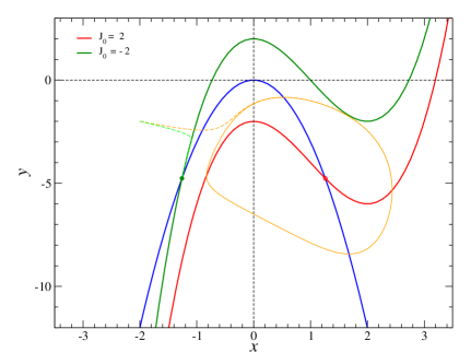
Figure 1: Nullclines for the system of Eq. 6 with $\beta=3$ and for $J_{0}$ values equal to $-2$ (green curve) and $2$ (red curve); the blue curve is the parabola given by the second formula of Eq. 7. Two phase trajectories (dashed lines) with the same initial conditions and corresponding to the two $J_{0}$ values are also shown: the green one moves along its nullcline to the stable equilibrium point (green filled circle) while the orange line describes a closed orbit around the unstable equilibrium point (red open circle).

This stability analysis shows that it depends upon the sign of the trace $Tr$ of the Jacobian of the system evaluated at $(x_{*},y_{*})$ (see Eq. 23). Fig. 2 shows the plots of $Tr$ as function of $J_{0}$ for two values of $\beta$, 3.0 and 4.0; the two vertical orange lines correspond to the zeroes of the trace and delimit the unstable interval for $\beta=3.0$, that, using the formulae given in Appendix B, results [0.0061792, 5.99382]. It is important to note that the instability interval depends only upon $\beta$ but not upon $J_{0}$; thus a change of this parameter moves the location of the equilibrium point allowing transitions between stable and unstable states. The above limits of the $J_{0}$ interval define the states at which the transition from stable to unstable equilibrium occurs, and therefore they rule the onset or the disappearance of the spiking behaviour. Examples of stable and unstable dynamical solutions are illustrated in Fig.1, where two trajectories corresponding to the values of $(x(t)$, $y(t))$ of the system in Eq. 6 are also plotted: they start from the same initial position, $x_{0}=-2.0$, $y_{0}=-2.0$, but, while the one for $J_{0}=-2.0$ reaches the green nullcline and then moves toward the corresponding equilibrium point, the other (orange trajectory) crosses the blue nullcline for $J_{0}=2.0$ and evolves to a closed orbit (limit cycle) around the unstable (red) equilibrium point (see Sect. 4.3).

It is interesting to note that the unstable interval for $\beta=3.0$ is [0.1835, 1.8165] and it is entirely contained in the interval [0, 2.0] corresponding to the portion of the $x$ nullclines with a negative slope, as it is easy to verify from the roots of the $x$ derivative of the first of Eq. 7.

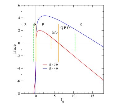
Figure 2: The plot of the traces of the Jacobian for two values of $\beta$ as function of the mean input $J_{0}$. Stable intervals ($\chi$, QPO) for the curve relative to $\beta=3.0$ are outside the vertical orange segments, and the unstable interval ($\rho$) is between them. Dashed lines within the stable and unstable regions mark the intervals in which other variability classes and behaviours are obtained as explicitly indicated in the graph.

4 Synthetic light curves

We show in this Section how the numerical solutions of the simplified system of Eq. 6 reproduce the main features of several variability classes and, particularly, four of them are obtained with a constant input level. Light curves are obtained by considering only the solutions for $x(t)$, which can be scaled by means of a linear transformation to the X-ray photon flux from the disc that is the main contributor to the luminosity in this band. Solutions for the other variable $y(t)$ will not be considered in the present paper and, in general, they could not directly be related to another observable quantity. However, one of the results, shortly presented in the Sect. 4.3.1, exhibits a high similarity with the disk inner radius as measured by Neilsen et al. (2012).

For some other classes, it is necessary to assume an input function variable on time scales similar to those detected in GRS 1915+105 light curves, with the exception of the spiking that is originated by non-linear instabilities. We will describe the analysis of the classes requiring a variable input in Paper II.

In this work, we limit our analysis to an input function $J(t)$ having the simple form:

$$J(t)=J_{0}+C~{}r$$ (8)

where $J_{0}$ is a constant component and $r$ is a random number with a uniform distribution in the interval [$-0.5$, $0.5$], $C$ the constant amplitude of random fluctuations and the resulting standard deviation $\sigma_{J}=C/(2\sqrt{3})$. The quantity $r$ is useful to simulate statistical fluctuations, as for instance those expected from turbulences in the disc, and to make our numerical results more similar to the observed ones. Of course, more realistic models would require the knowledge of the turbulence spectrum, that is not yet determined. The physical interpretation of $J_{0}$ is not apparent in this formulation: in Massaro et al. (2014), we assumed that it may be related to the local mass accretion rate $J(\dot{m})$, but this hypothesis will be newly reconsidered in the present and in Paper II on the basis of the MHR results.

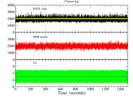
Figure 3: Top: segment of a RXTE/PCA light curve of the $\chi$ class (ID 10408-01-22-02) in the 2-12 keV energy interval, the horizontal yellow belt around the mean level is the mean amplitude expected from Poisson noise. Centre: model light curves obtained by a numerical solution of Eq. 6 using as input function the curve in the bottom panel. Bottom: input function consisting of the superposition of a constant level $J_{0}=-$3.0, equal to the mean value represented by the dark green horizontal line, and a white random noise given by $C=4.0$.

The other parameter to be determined is $\beta$. Considering that we used a linear transformation to scale our numerical results to the actual time and amplitude of the light curves, we decided to use parameters’ value in a range between 0 and 10, to manipulate small numbers which reduce the possibility of numerical troubles in the numerical integration. From our results, we found that a $\beta$ value between 3.0 and 4.0 gives solutions in good agreement with the data: the higher value producing spikes slightly narrower than those obtained with the lower one while no apparent difference is found for the stable light curves. In the following we will present the results obtained assuming $\beta=3.0$ because transitions between different variability classes are obtained for $J_{0}$ changes within a rather narrow range, as explained in Appendix B. The values of this parameter used for computing the following light curves are given in Table 1. However, in Paper II we will show that a few classes of light curves are better reproduced for different choices of this parameter. The amplitude of the random fluctuating component was generally fixed to $C=4.0$, while the value 3.5 was considered in Sect. 6 for investigating the QPO origin.

For the comparison of MHR results with data we used several RXTE/PCA observations selected as examples of the considered classes. The light curves are accumulated with standard procedures in the energy range 2-12 keV.

4.1 Classes $\phi$, $\chi$

Light curves of these two classes are characterised by a rather stable or slowly variable mean level with fluctuations typical of a statistical noise. The main difference between these two classes is in the hardness ratio and this changes are not taken into account in our mathematical modelling that is limited to reproduce the observed patterns of the X-ray light curves in the energy range 2-12 keV, dominated by the disc emission. As an example, an observed light curve relative to the class $\chi$ is shown in the top panel of Fig. 3. Note that fluctuations in the light curve are much higher than the Poissonian noise associated with the observed counts, whose mean amplitude is represented by the yellow strip around the mean count level. These fluctuations could be originated by fast random changes intrinsic to the disc as one can expect from plasma turbulence or other similar stochastic processes.

In Fig. 3, the observed light curve is compared with the output of the MHR model of Eq. 6 for $J_{0}=-3.0$ and the corresponding input function $J(t)$ is represented by the green data series in the bottom panel where the darker line indicates the mean value. Fluctuations in the computed values are clearly due to the random white noise and, for $C=0$, they are absent and a constant equilibrium solution is obtained.

We note that the MHR model reproduces the $\phi$ and $\chi$ classes when $J_{0}$ is increased up to values high enough that the equilibrium point is again in a stable region ($J_{0}>6$), however this transition from the unstable region to the stable one implies the disappearance of the limit cycle and the onset of a QPO phenomenon as shown in Sect. 6.

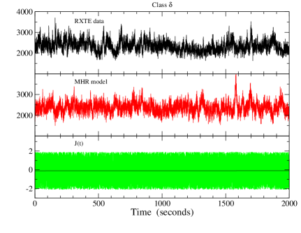
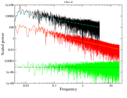
Figure 4: Upper plot: segment of a RXTE/PCA light curve of the $\delta$ class (ID 10408-01-13-00) in the 2-12 keV energy interval (black curve in the top panel); light curve obtained by means of the MHR model (red curve in the central panel) using as input function the green curve in the bottom panel obtained by the superposition of a white random noise $C=4.0$ to a constant level $J_{0}=-0.1$; the mean value is represented by the dark green horizontal line.
Lower plot: power density spectra of the $\delta$ light curves in the upper plot, for the observed data (black), for the curve computed with the MHR model (red) and for the input $J(t)$ (green). The dashed cyan, orange and dark green lines are the relative power law best fits.

4.2 Class $\delta$

According to Belloni et al. (2000), light curves of the $\delta$ class appears to have a rather stable mean level but with a red noise-like variability. Very similar results are obtained by means of the MHR model when the $J_{0}$ value increases approaching to 0. RXTE data and a computed light curve are shown in top and centre sections of the upper panel in Fig. 4, respectively. We can use these curves to apply the Fourier analysis and evaluate the Power Density Spectrum (PDS) that indeed presents a red noise with a power law distribution having the exponent equal to $-1.1$, remarkably close to the one of the true data that is $-0.91$, while that of the input $J(t)$ corresponds to a flat white noise (Fig. 4, lower panel). We can therefore conclude that the non linearity of the MHR model also acts as a red noise generator, when the equilibrium points approaches the instability region. Also for this class the assumption $C\neq 0$ is necessary to obtain these patterns. Eliminating the noise the MHR solution is a constant equilibrium value which changes to a small amplitude oscillation and to the spiking behaviour for increasing $J_{0}$.

As shown in the following subsection a further increase of $J_{0}$ will produce $\rho$ class light curves. The $\delta$ class should therefore be considered as a transition class between the $\chi$ and $\rho$ classes.

Table 1: Parameters’ values adopted in the numerical calculations of the light curves for the variability classes of GRS 1915+105.

Class	$\beta$	$C$	$J_{0}$
$\chi$	3.0	4.00	$-$3.0
$\delta$	3.0	4.00	$-$0.1
$\rho_{d}$	3.0	4.00	0.05
$\rho$	3.0	4.00	0.80

4.3 Classes $\rho$, $\rho_{d}$

The class $\rho$ is likely the most interesting and the most studied one: it consists of nearly regular series of spikes with a recurrence time variable in the range from about 40 s to more than 100 s; the shape of the spikes is characterised by an initial rather slow rise followed by a faster increase and a similarly fast decline (see Fig. 5). Moreover, in several cases the spikes have a double or even a multiple structure. Massaro et al. (2010) introduced a multiplicity parameter $p$ to number the peaks apparent in the fine structure and Yan et al. (2017)Yan et al. (2017) defined the ‘subclasses’ $\rho_{1}$ and $\rho_{2}$ corresponding to $p$ equal to 1 or 2, which are the most frequent patterns. We here introduce another subclass $\rho_{d}$, which has spikes similar to those of the typical $\rho$ one, but with the occurrence of a dip just at the their end, frequently followed by a fast rise and a plateau preceding a new fast rise of the following peak (see Fig. 6). The $\rho_{d}$ mean recurrence time is usually longer than that of $\rho$ spikes. This subclass was the first one observed by Taam et al. (1997), who reproduced its main features by computing the light curve due to the disc instability previously investigated by Taam & Lin (1984).

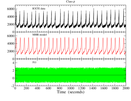
Figure 5: Top: segment of a RXTE/PCA light curve of the $\rho$ class observation ID 20402-01-31-00 in the 2-12 keV energy interval; Central: light curve obtained with the MHR model using the input curve plotted in the bottom panel; Bottom: input function $J(t)$, with random fluctuations obtained with $C=4.0$ superposed to a constant value $J_{0}=0.8$; its mean value is the dark green line.

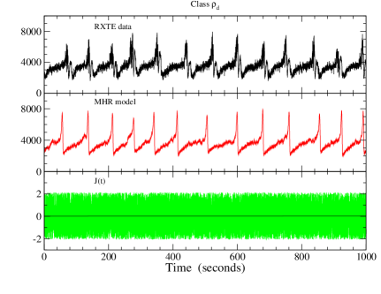
Figure 6: Top: segment of a RXTE/PCA light curve of the $\rho_{d}$ class of the observation ID 10408-01-41-00 in the 2-12 keV energy interval. Central: light curve (red) obtained with the MHR model using the input model in the bottom panel. Bottom: input function $J(t)$ with random fluctuations obtained with $C=4.0$ superposed to a constant value $J_{0}=0.05$; its mean value is the dark green line.

Our mathematical model is able to produce a spiking behaviour when the mean $J(t)$ is further increased above the stability threshold: a transition from stable to unstable equilibrium occurs and a limit cycle is established. A similar behaviour was also found for the FitzHugh-Nagumo model analysed in Massaro et al. (2014) and Ardito et al. (2017). Fig. 5 and Fig. 6 (middle panel) show the spiking behaviour of the main class and of the subclass that are remarkably similar to the observed ones. The variable recurrence time of spikes, clearly apparent in the data panel in Fig. 5 (top panel), can be due local changes of the mean level of $J(t)$, as it will be discussed in detail in the following section. Peaks in the $\rho_{d}$ data have generally a double structure, as already noticed by Taam et al. (1997) and in other observations the $\rho$ peaks exhibit also a more complex fine structure (see, for instance, Belloni et al., 2000; Massaro et al., 2010). Here we modelled only a single peak pattern and these more structured profiles require some other assumption on the input function. Note also that this light curve is more irregular than the one of the $\rho$ class; moreover, its $J_{0}$ is slightly lower and therefore it appears as a transition between the $\delta$ and the $\rho$ classes.

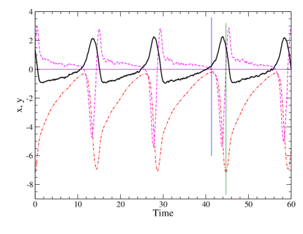
Figure 7: Numerical solutions of the variable $y(t)$ (red curve) and its first derivative (magenta curve) compared with the $x(t)$ (black curve) when in the $\rho$ spiking class. The blue and green vertical lines limit the interval between a maximum and a minimum of $y(t)$ where it is very quickly decreasing that corresponds to the highest emission in the $x(t)$ peak. The violet horizontal line marks the zero level.

4.3.1 The $y$ variable

For a better understanding of the solutions for the $\rho$ class it is useful to consider the behaviour of the $y$ variable and of its time derivative. With the adopted parameters’ values, Eq. 4 becomes:

$$\frac{dx}{dt}=-x^{3}-\frac{dy}{dt}+J(t)$$ (9)

that shows the relevant role of the $y$ derivative in the evolution of the burst profile.

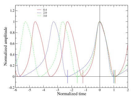
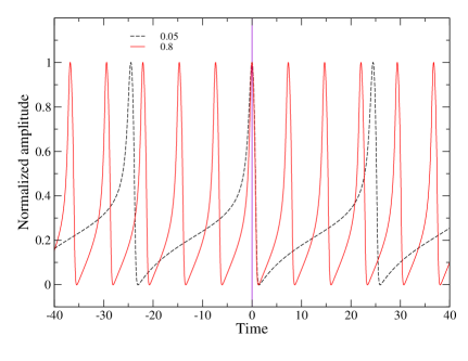
Figure 8: Upper plot: Normalized profiles of three spikes of the $\rho$ class obtained by the MHR model for three values of $J_{0}$ without the random component. Vertical bars mark the initial and final points of the corresponding colour spikes. Curves, after the subtraction of the minimum level, are normalized in amplitude by taking the maximum value equal to unit, and in time by fixing to 1.0 the duration of the interval between the maximum and the end point of the spike for $J_{0}=2.0$ (blue line).
Lower plot: comparison between results for a typical $\rho$ (red) and a $\rho_{d}$ (black) profile obtained for a $J_{0}$ close to the stability boundary.

Fig. 7 shows the numerical solutions for $y(t)$ and its derivative corresponding to the $\rho$ bursting sequence of $x$. In this case, the variables’ values are not scaled to the measured count rates and no constant offset was added, as in Fig. 1. The profile of $y$ consists of an initially fast increase followed by a milder hump up to the maximum and then by a sudden and very fast decrease. This shape is very similar to the one found by Neilsen et al. (2012) (see their Fig. 6) for the inner radius of the accretion disc in the time resolved spectral analysis of the $RXTE$ observation 40703-01-07-00, performed using the model developed by Zimmerman et al. (2005, ezdiskbb in XSPEC ). The two vertical lines in Fig. 7 limit one of the decreasing intervals, where the $y$ derivative is negative, to show that it corresponds to the interval of the peak in the $x$ curve. Again, there is a similar phase shift between the maxima of the two variables as in those of Neilsen et al. (2012). We recall that, in the emission models, the luminosity is proportional to the square of the inner radius and therefore it can exhibit variations with the same time scales. This correspondence supports the association of the $y$ with a disc quantity which follows a limit cycle as the luminosity. In the discussion of Paper II we will present a possible interpretation to be verified by means of calculations of thermal-viscous instabilities.

5 Structure and period of the $\rho$ class spikes

The two qualifying observable quantities of the $\rho$ class spiking are the profile and the recurrence time of spikes. Several observations (see, for instance, Neilsen et al., 2011; Weng et al., 2018) have shown that the spike structure is highly variable and that it frequently can exhibit two or more peaks. However, in many occasions and over time intervals of several thousands of seconds, the mean profile appears to be stable (Massaro et al., 2010). The solutions of the MHR model, whitout any random component in $J(t)$, give smooth and stable profiles with a duration, and consequently the recurrence time, depending upon $J_{0}$. Three profiles, computed for $J_{0}$ in the range [0.4, 4.0], are shown in the upper plot of Fig. 8. For a better comparison of these profiles we subtracted the constant offset level and normalized the maxima to unity. Moreover, the time distance between the maximum and the end of the spike was fixed also to unity for the longest one ($J_{0}=0.4$, red curve), and then we used this scale factor for reducing the periods of the other two profiles which where aligned at the time of the maximum. One can see that the change of the spike duration is mainly due to the rising section, while the decaying part remains more stable, slightly increasing with $J_{0}$. It follows that spikes evolve to be more symmetric when the recurrence time decreases. In practice, one can consider that for $J_{0}\gtrsim 4.0$ the spiking behaviour changes to a nearly sinusoidal high frequency oscillation (hereafter ‘hfo’) whose frequency changes very little for further increases of $J_{0}$.

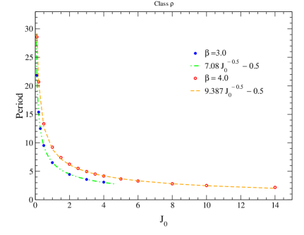
Figure 9: The period of spikes in the $\rho$ class for two values of $\beta$ as function of $J_{0}$. Blue and red circles are the results of numerical calculations, while the dashed lines are the best fit interpolations with a fixed exponent.

It is also interesting to see how spike profiles change when the values of $J_{0}$ are just above the stability boundary and produce the $\rho_{d}$ pattern. This comparison is shown in the lower panel of Fig. 8, where two normalised MHR results are plotted. Again major differences are in the rising segment of the spike: in the $\rho_{d}$ case it starts with a high slope that decreases and turns to increase again to reach the maximum. This particular shape can be affected by fluctuations which can amplify the slope changes moving the input value across the stability threshold, thus producing the dips at the spikes’ end, which are thus explained by the non-linear dynamics of disc oscillations.

The changes of the recurrence time, essentially due to the variable duration of the rising part of spikes, are thus explained by the occurrence of a slow and a fast time scale, as occurs in the limit cycles of non-linear oscillators.

A very interesting property of the $\rho$ class spikes is that their periodicity depends on the value of $J_{0}$. To obtain a functional relationship we computed several light curves, without the random component (i.e. fixing $C=0.$ in Eq. 8), for $J_{0}$ values ranging from 0.1 to 4.0 and two values of $\beta$. The spike period was then evaluated by means of a Fourier periodogram and the resulting values are plotted in Fig. 9. A very well defined and regular decreasing trend is clearly apparent that is described either by a simple power law:

$$P(J_{0})=K(\beta)~{}J_{0}^{-s}$$ (10)

For both $\beta$ values the resulting exponent was $s=0.535$, very close and only slightly different than 0.5. We then fixed the exponent to this value and included an additional constant term in the best fitting formula:

$$P(J_{0})=K(\beta)~{}J_{0}^{-0.5}+q~{}~{}~{}~{}~{}~{}.$$ (11)

The resulting regression function are practically coincident with those Eq. 11 and $q$ was found so very close to $-0.5$, that we decided to freeze it at this value leaving only $K(\beta)$ as free parameter. The final curves and their best fit laws are given in Fig. 9. Note that for both laws the ratio $K(4)/K(3)\approx 4/3$, suggesting that $K(\beta)$, at least in this rather narrow range, may be linear, but more calculations are necessary to unravel this dependence. We expect, therefore that a slowly modulated $J(t)$ would result in a change of the the mean recurrence time between spikes.

6 The origin of low frequency QPOs

In the previous sections, we showed that the MHR model reproduces the sequence of classes $(\phi,\chi)\rightarrow\delta\rightarrow\rho$ for increasing values of $J_{0}$ as illustrated by Fig. 2. When $J_{0}$ increases, the recurrence time of $\rho$ spikes decreases (see Fig. 9), and their profiles become more and more symmetrical up to approximate a sinusoidal ‘hfo’ pattern, whose amplitude is slightly variable because of the fast random changes of $J(t)$. Some examples of light curves are shown in the three upper panels in Fig. 10. A further increase of $J_{0}$ produces a transition to the second stable region (see Fig. 2) thus we expect a signal rapidly evolving to a constant level, however, the occurrence of fast fluctuations of $J_{0}$ in the unstable region determines a random appearance of ‘hfo’ with an amplitude modulation which sets on longer time scales (bottom panel in Fig. 2). The PDS (Fig. 11) of this light curve shows a broad feature, typical of QPOs frequently found in binary X-ray sources and, in particular, in low mass X-ray binaries hosting a Black Hole or a Black Hole candidate, like GRS 1915+105. Finally, as discussed previously, when $J_{0}$ reaches values high enough that the equilibrium point remains always in the stable region, the structure of the light curve results again that of the $\chi$ class.

van den Eijnden et al. (2016) applied an optimal filtering to the GRS 1915+105 light curves to obtain the structure of the signal in the frequency band of the QPO. The resulting shape (see Fig. 4 in their paper) is that of a periodic oscillation whose amplitude is modulated by a non periodic pattern with a time scale higher than that of the oscillation by a factor of between about 5 and 10. It is interesting to note that this filtered signal turns out remarkably similar to the one plotted in the bottom panel in Fig. 10.

On the basis of these results it is possible to formulate an hypothesis on the origin of QPO in an accretion disc. They are essentially related to the same mechanism responsible of the spiking limit cycle but appears at a transition between the unstable and the stable region for high $J_{0}$. Random or turbulence fluctuations may be responsible for the alternance between the two regions thus producing the amplitude modulation of the oscillations.

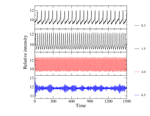
Figure 10: Light curves computed applying the MHR mathematical model assuming $J(t)$ of Eq. 8, with $C=3.5$ and different $J_{0}$ to change the position of the equilibrium point from the unstable to the stable region. The values of $J_{0}$ from top to bottom are 0.3, 1.5 ($\rho$ class), 4.0 (hfo), 6.5 (QPO).

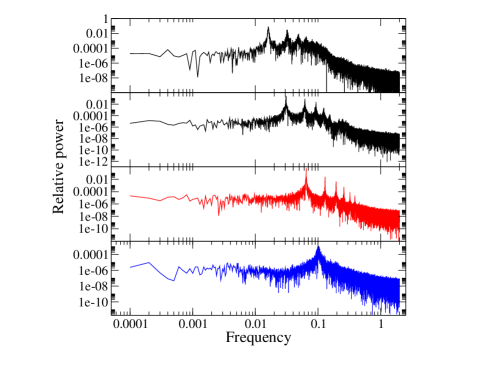
Figure 11: Power density spectra of the light curves in Fig.10. The two upper panels correspond to the spiking of the $\rho$ class, while the third panel (red curve) is that of the ‘hfo’. All these spectra are dominated by the narrow lines and their harmonics of the periodic signals. The blue spectrum in the last panel has a unique broad peak typical of a QPO.

6.1 Structure of the QPO feature

We performed additional numerical calculations to verify how the structure of the QPO feature in the PDS depends upon $J_{0}$. We considered the two following cases: $i$) a $J_{0}$ value just above the upper boundary of the unstable region (see Sect. 3 and Appendix B), namely 6.1, in order to have about 50% of $J(t)$ values in the unstable region, because of the random fluctuations, and $ii$) $J_{0}=7.5$, so that only about 7% of them are in this region. The time scale of these signals was established to have QPO frequencies near 1 Hz. Two short segments of light curves are reported in the upper plot of Fig. 12 from which clearly results the presence of a modulated ‘hfo’ with amplitudes depending upon $J_{0}$ being larger when this quantity is just above the boundary, while the other resembles to one of $\chi$ class. Their PDS are given in the lower plot: large QPO features are in both spectra at very close frequencies, namely 0.965 and 1.10 Hz, but the one for $J_{0}=6.1$ is more prominent and at least two harmonics are apparent. Note the high similarities between these results and the spectra reported by Stiele & Yu (2014) for three RXTE observations in the energy band 4.9 - 14.8 keV. Profiles of both features can be well described by Lorentzian functions from which one can estimate their Q factors that result 5.8 and 29.2. These values are also dependent on the amplitude of random component, because when it is reduced to 0, the light curve, after a rather fast transient, reaches a constant. Of course a further increase of $J_{0}$ would continue to reduce the value of Q up to the complete quenching of the QPO.

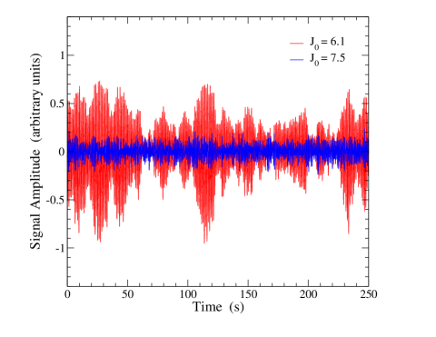
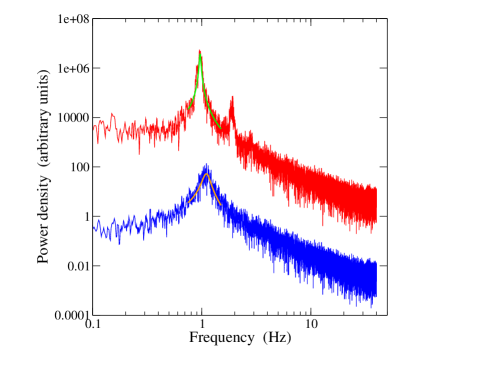
Figure 12: Upper plot: Light curves computed applying the MHR mathematical model assuming $J(t)$ of Eq. 8, with $C=3.5$ and two values of $J_{0}=6.1$ (red curve), just higher than the transition level and 7.5 (blue curve), both located in the stable region. Lower plot: power density spectra of these curves, shifted to separate the profiles of QPO features. The green and oranges thick curves are the Lorentzian fits of the QPO peaks.

7 Summary and discussion

It is known from the study of dynamical systems (see, e.g Strogatz, 1994) that the development of convective energy transport and chaotic turbulent motions in a fluid can be described by systems of non-linear equations, as e.g. the very famous one due to Lorenz (1963). In the astrophysical contest Arnett & Meakin (2011) applied Lorenz equations to investigate recurrent fluctuations in turbulent kinetic energy in a stellar oxygen burning shell.

We used a similar approach and derived the MHR model, based on a system of two ODEs, whose results have shown that some complex patterns, like those exhibited by GRS 1915+105, are well described by non-linear processes and by transitions between stable and unstable states driven by a single input function $J(t)$. Synthetic light curves remarkably very similar to those of $\phi$, $\chi$ and $\delta$ classes are obtained in conditions of a stable equilibrium and a constant input added to random fluctuations as reasonably expected in a turbulent hot plasma. The $\delta$ class requires that the mean input would be close to stability threshold (in our simple case it is close to $J_{0}=0$) and its detailed structure depends upon the amplitude and time scales of input fluctuations, whose values could exceed the unstable interval boundary. The MHR equations thus introduce correlations in the output over time scales longer than the one of fluctuations and originate a red noise PDS. The idea of considering a non-linear ODE for describing some properties of accretion disc oscillations was already adopted by other authors: for instance, Ortega-Rodríguez et al. (2014) considered the harmonic oscillator equation including quadratic and cubic terms and a sinusoidal forcing for describing the spectral structure of the normal mode oscillations in a thin accretion discs.

An outstanding feature of the MHR model is its ability to produce a spiking state, again very similar to the $\rho$ class signals, without the introduction of any ad hoc assumption on the time variations of the accretion rate or any other physical quantity of the accretion processes. This capability is also for other simpler ODE systems, like the FitzHugh-Nagumo model presented in Massaro et al. (2014), but the solutions obtained by means of MHR model are able to better describe the transitions between some classes and have therefore a higher heuristic content. The shape of spikes is well reproduced also in the cases where a dip appears just after the end of the peak, characteristic that we used to define the $\rho_{d}$ subclass. The condition to produce this pattern is that the fluctuations with respect to a stable value of the input function move its value across the instability boundary and interrupt the completion of the limit cycle making the spike separation highly irregular. Both these transition effects induced by noise can be easily verified by eliminating the fluctuations (i.e. fixing $C=0$) and obtaining purely stable or spiking solutions, as shown in Sect. 5. An important property of the spiking is the dependence of the recurrence time on the length of the rising segment while the peak width remains practically stable, in a very good agreement with the observational results (Massaro et al., 2014; Massaro et al., 2010).

To make clear how the MHR model can develop the limit cycle of the $\rho$ class it is useful to consider the single ODE given in Eq. 17:

$$\ddot{x}+F(x)\dot{x}+x^{3}-J_{0}=0~{}~{}~{}~{}.$$ (12)

It is easy to verify that, after a multiplication by $\dot{x}$, it can be transformed into the equivalent form:

$$\frac{dE}{dt}=-\dot{x}^{2}F(x)~{}~{}~{}~{}~{}~{},$$ (13)

where

$$E(x,\dot{x})=\frac{1}{2}\dot{x}^{2}+\int(x^{3}-J_{0})dx~{}~{}~{}~{}~{}~{}.$$ (14)

In the case that $F(x)$ is always positive or negative, the quantity $E$ will be indefinely decreasing or increasing, respectively; these two situations correspond either to the approach to stable equilibrium or to an unstable diverging amplitude. If $F(x)$ has both positive and negative values, one can have an alternance between damping and excitation and $E$ and $x$ have an oscillating behaviour, that is named ‘self-excited’, because of the absence of any periodic forcing.

In our case $F(x)$ is a second degree polynomial equal to the opposite of the trace of the Jacobian (see Appendix  B), and therefore for $\beta^{2}>3$ there are real zeros, then the sign of $F(x)$ can change and self-excited oscillations are possible. For $\beta^{2}<3$ the values of $F(x)$ are all negative and the solution converge rapidly to equilibrium.

A limitation of MHR model, at least in the present version, is that it does not take into account the dependence of the spiking profiles on the photon energy. We know from a previous analysis that the full width half maximum of spikes decreases with energy following a relationship close to a power law with an exponent $\approx 0.8$ (Maselli et al., 2018). The model light curve for the $\rho$ class shown in Fig. 5 has therefore a spike FWHM corresponding to an intermediate energy in the considered range, depending upon the instrumental response. We did not include any parameters in the MHR model to account for the energy dependent properties of the light curves. A change of the ODE system including more terms and more parameters will make the stability analysis of solutions much harder than in our case.

A serendipitous and very interesting result of the MHR model presented in Sect. 6 is the occurrence of low-frequency QPOs when the system reaches the stable region for high $J_{0}$ values. For increasing $J_{0}$ the limit cycle evolves towards the region of ‘hfo’, whose frequency is rather stable and changes very little as shown in Fig. 9. QPOs are due to amplitude modulation of these ‘hfo’ on time scales much longer than their period. It is interesting that the model reproduces quite well the amplitude modulation resulting in the data applying an optimal frequency filtering as shown by van den Eijnden et al. (2016). An alternative possibility was proposed by Suková & Janiuk (2015) who investigated the time evolution of shock oscillations by means of numerical hydro-dynamical simulations: their solutions for the accretion rate exhibit patterns similar to hfo and could be also associated with low-frequency QPOs. However, a connection of the Suková & Janiuk (2015) model with the limit cycle of the $\rho$ class is not established. According our results, the same processes generating the spiking limit cycles around an unstable equilibrium point is also responsible of QPOs, but in this case the disc structure remains in a stable condition for most of the time. This is probably the general condition of the other low mass X-ray binary accretion discs that generally shows QPOs or red noise. A more detailed study of non-linear mechasmims for producing QPOs and the relevance of the noise will be investigated in a further work.

It is useful to distinguish between low and high-frequency QPO. As written above, our results suggest that the low-frequency QPOs, typically in the range from a fraction to a few Hz (Yan et al., 2017), can be related to the changes of a noisy input function across the border between unstable and stable equilibrium region, while high-frequency QPOs can originate by a different physical mechanism that likely involves local oscillations and waves in the disc. Hydrodynamic calculations (Reynolds & Miller, 2009) for a thin accretion disc have shown that turbulence does excite QPOs whose PDS has a red continuum with a broad peak at frequencies close to the radial epicyclic frequency at $\nu_{re}\approx 10^{3}(M_{\odot}/M)$ Hz where $M$ is the central black hole mass. In the case of GRS 1915+105 the estimated mass of about 12 $M_{\odot}$ (Reid et al., 2014) and the resulting $\nu_{re}\approx 80$ Hz are therefore comparable to those of the observed high frequency QPOs (Belloni & Altamirano, 2013).

As already noticed above for the $\rho$ class, the present version of MHR model is not able to describe the properties of low frequency QPOs depending on energy as those reported by various authors (e.g. Stiele & Yu, 2014; Zhang et al., 2015; Ingram & van der Klis, 2015). Again an extended model with more parameters is necessary, but reasonably one could expect more complex stability conditions for deriving the various light curves of various classes and transitions between them.

An important subject emerging from our modelling is the fundamental role of the spectrum of the plasma turbulence in the disc. Some classes, like $\chi$ and $\delta$, and QPOs are obtained by the MHR model only if a noise contribution is considered. For what concerns the amplitude distribution we made the simplest assumption of a random white noise, variable step by step, and with a uniform distribution in the interval [$-C/2$, $+C/2$]. A more realistic noise model will have to take into account the probability distribution function produced by turbulent motions in the disc, as for instance a log-normal law that, considering the energy dissipation in Alfvenic turbulence, well describes the statistical properties of this phenomenon (see Zhdankin et al., 2016). The relevance of turbulence in disc dynamics has been recently investigated by Ortega-Rodríguez et al. (2020), who pointed out that stochastic oscillations can behave as a driving agent for producing the twin peak structure of high frequency QPOs.

Light curves obtained by means of the MHR model are not limited to those described in the present paper which were all computed using a constant $J_{0}$. It is possible to show that structures as those of several other classes (for instance $\alpha$, $\gamma$, $\lambda$, $\kappa$, $\omega$, $\xi$, $\theta$) result when this assumption is relaxed and a step function or sawtooth modulations of $J(t)$ on the proper time scales are introduced. The extension of MHR model to other variability classes will be discussed in detail in Paper II.

The physical meaning of the input function $J(t)$ is likely related to some parameter affecting the disc state and consequently its brightness and stability. In the paper concerning the FitzHugh-Nagumo model Massaro et al. (2014) proposed that it is related to the mass accretion rate in the disc. This hypothesis remains useful also in the context of the MHR model but it requires a further analysis to establish a reliable functional form. In particular, one could use the large collection of observation to search for correlations between the properties of the various variability classes and the mean luminosity and its changes or some other spectral parameter. This draining work is beyond the goals of the present paper that is focused on the development of a tool for simulating the stability conditions that produce the rich collection of variability classes.

A more detailed comparison between our MHR model and these disc instabilities will be given in Paper II.

Appendix A The differential equation for x

The ODE system of Eq. 3, or that of Eq. 6, can be reduced to a single ODE for the variable $x$ by eliminating $y$ and $\dot{y}$; deriving the first ODE in Eq. 3, we have:

$$\ddot{x}=(-3\rho x^{2}+2\beta_{1}x)\dot{x}+\dot{y}+\dot{J}(t)$$

and using the equations for $\dot{y}$, it follows

$$\ddot{x}=(-3\rho x^{2}+2\beta_{1}x)\dot{x}-\beta_{2}x^{2}-y+\dot{J}(t)~{}~{}~{}~{}.$$

Then one can use the ODE for $\dot{x}$ to eliminate $y$, and the final result is

$$\ddot{x}+F(x)\dot{x}-(\beta_{1}-\beta_{2})x^{2}+\rho x^{3}-[J(t)+\dot{J}(t)]=0$$ (15)

where

$$F(x)=3\rho x^{2}-2\beta_{1}x+1~{}~{}~{}~{}.$$ (16)

In the simple case with $\beta_{1}=\beta_{2}$, $J(t)=J_{0}$, and $\rho=1$ (with no loss of generality), it becomes:

$$\ddot{x}+F(x)\dot{x}+x^{3}-J_{0}=0~{}~{}~{}~{}.$$ (17)

Another simple derivation of this equation is obtained by introducing the new variable:

$$w(t)=x(t)+y(t)~{}~{}~{};~{}~{}~{}\dot{w}=\dot{x}+\dot{y}~{}~{}~{}$$

and adding the two equations for $\dot{x}$ and $\dot{y}$ we have:

$$\frac{dx}{dt} = -x^{3}+\beta~{}x^{2}-x+w+J_{0}$$

$$\frac{dw}{dt} = -x^{3}+J_{0}$$ (18)

This ODE system is equivalent to the MHR of Eq. 3, but the second variable is different. Deriving the equation for $\dot{x}$ and using that for $\dot{w}$ we obtain again the previous Eq. 17.

Appendix B Nullclines, equilibrium points and instability interval

Let us consider the model of Eq. (3), with $\rho=1.0$ without loss of generality

$$\frac{dx}{dt} = -x^{3}+\beta_{1}x^{2}+y+J(t)$$

$$\frac{dy}{dt} = -\beta_{2}x^{2}-y$$ (19)

It is possible to demonstrate that if $J(t)$ is a bounded function, $|J(t)|\leq M,\forall t$, also the solutions for $x(t)$ and $y(t)$ are bounded.

Lemma: If $J(t)$ is bounded then exists a number $b>0$, such that for any initial condition $(x(0)$, $y(0))$ it exists a value $\bar{t}>0$ such that $\|x(t)$, $y(t)\|\leq b$, $\forall t>\bar{t}$.

Proof: Let $V(x,y,t)=(1/2)(x^{2}+y^{2})$ then

$\dot{V}=-x^{4}+\beta_{1}x^{3}+xy+xJ(t)-\beta_{2}x^{2}y-y^{2}\leq G(x,y)$

where

$G(x,y)=-x^{4}+\beta_{1}x^{3}+xy-\beta_{2}x^{2}y-y^{2}+|x|M$,

and using polar coordinates it is easy to verify that

$$\lim_{x^{2}+y^{2}\rightarrow+\infty}G(x,y)=-\infty~{}~{}.$$

To study the stability conditions of the ODE system in Eq. (4) with $J(t)=J_{0}$ we consider the system

$$\frac{dx}{dt} = -x^{3}+\beta~{}x^{2}+y+J_{0}$$

$$\frac{dy}{dt} = -\beta x^{2}-y$$ (20)

Thus its nullclines are given by the equations:

$$y = x^{3}-\beta~{}x^{2}-J_{0}$$

$$y = -\beta~{}x^{2}$$ (21)

which admits the unique real equilibrium point $x_{*}=J_{0}^{1/3}$, $y_{*}=-\beta~{}J_{0}^{2/3}$. To investigate local the stability of this solution we perform the linear analysis at $x_{*}$ by means of the sign of the determinant and trace of the Jacobian:

$$\left(\begin{array}[]{cc}-3x_{*}^{2}+2\beta x_{*}&1\\ -2\beta x_{*}&-1\end{array}\right)$$

whose determinant $\Delta$ is

$$\Delta=3x_{*}^{2}-2\beta x_{*}+2\beta x_{*}=3x_{*}^{2}\geq 0$$ (22)

is non-negative while the sign of the trace is given by the roots of:

$$-3x_{*}^{2}+2\beta~{}x_{*}-1=0$$ (23)

which are $x_{*1,2}=(\beta\pm\sqrt{\beta^{2}-3}~{})/3$. The local unstable equilibrium condition $Tr>0$ corresponds to values of $x_{*}$ within the interval $I\equiv[(\beta-\sqrt{\beta^{2}-3}~{})/3$, $(\beta+\sqrt{\beta^{2}-3}~{})/3]$.

For a general analisys of the stability one can introduce the Lyapunov function

$$V(u,v)=(u^{2}/4)(u^{2}+4x_{*}u+6x_{*}^{2})+(v^{2}/2)$$

where $u=x-x_{*}$, $v=(x-x_{*})+(y-y_{*})$. It is easy to verify that: $i$) for $\beta^{2}\leq 3.0$ and $x_{*}\notin I$, one has $\dot{V}\leq 0$ and therefore the equilibrium is globally stable; $ii$) for $\beta^{2}>3.0$, and $x_{*}\leq\xi_{1}$ or $x_{*}\geq\xi_{2}$, with $\xi_{1,2}=(\beta\pm 2\sqrt{\beta^{2}-3}~{})/3$, one has again $\dot{V}\leq 0$ and the equilibrium is globally stable. For $x_{*}\in I$, considering that the solution is bounded, one has at least a periodic orbit.

In the case of $x_{1}\char 60\relax x_{*}\char 60\relax x_{2}$ we can prove that if $\beta^{2}\char 62\relax 3$, and if $x_{*}^{3}=(1/27)\beta(2\beta-3)$ then the periodic orbit is orbitally stable and therefore it is unique (see Coppel, 1965; Hale & Kojak, 1991).

References

- Abramowicz et al. (1988) Abramowicz M. A., Czerny B., Lasota J. P., Szuszkiewicz E., 1988, ApJ, 332, 646
- Abramowicz et al. (1995) Abramowicz M. A., Chen X., Kato S., Lasota J.-P., Regev O., 1995, ApJ, 438, L37
- Ardito et al. (2017) Ardito A., Ricciardi P., Massaro E., Mineo T., Massa F., 2017, International Journal of Non Linear Mechanics, 88, 142
- Arnett & Meakin (2011) Arnett W. D., Meakin C., 2011, ApJ, 741, 33
- Belloni & Altamirano (2013) Belloni T. M., Altamirano D., 2013, MNRAS, 432, 19
- Belloni et al. (2000) Belloni T., Klein-Wolt M., Méndez M., van der Klis M., van Paradijs J., 2000, A&A, 355, 271
- Buchler (1993) Buchler J. R., 1993, Ap&SS, 210, 9
- Buchler & Regev (1981) Buchler J. R., Regev O., 1981, ApJ, 250, 776
- Castro-Tirado et al. (1992) Castro-Tirado A. J., Brandt S., Lund N., 1992, IAUC, 5590, 2
- Chen & Taam (1993) Chen X., Taam R. E., 1993, ApJ, 412, 254
- Coppel (1965) Coppel W., 1965, Stability and asymptotic behavior of differential equations. Heath Mathematical Monographs
- Fender & Belloni (2004) Fender R., Belloni T., 2004, ARA&A, 42, 317
- FitzHugh (1961) FitzHugh R., 1961, Biophysical Journal, 1, 445
- Gerstner et al. (2014) Gerstner W., Kistler W. M., Naud R., Paninski L., 2014, Neuronal Dynamics. Cambridge University Press
- Hale & Kojak (1991) Hale J., Kojak H., 1991, Dynamics and Bifurcation. Springer Verlag, New York
- Hannikainen et al. (2003) Hannikainen D. C., et al., 2003, A&A, 411, L415
- Hannikainen et al. (2005) Hannikainen D. C., et al., 2005, A&A, 435, 995
- Hindmarsh & Cornelius (2005) Hindmarsh J. L., Cornelius P., 2005, 2005, BURSTING: The Genesis of Rhythm in the Nervous System. S. Coombes & P.C. Bressloff eds
- Hindmarsh & Rose (1984) Hindmarsh J. L., Rose R. M., 1984, Proceedings of the Royal Society of London Series B, 221, 87
- Honma et al. (1991) Honma F., Matsumoto R., Kato S., 1991, PASJ, 43, 147
- Huppenkothen et al. (2017) Huppenkothen D., Heil L. M., Hogg D. W., Mueller A., 2017, MNRAS, 466, 2364
- Ingram & van der Klis (2015) Ingram A., van der Klis M., 2015, MNRAS, 446, 3516
- Izhikevich (2006) Izhikevich E. M., 2006, Dynamical Systems in Neuroscience:The Geometry of Excitability and Bursting. MIT Press
- Janiuk et al. (2000) Janiuk A., Czerny B., Siemiginowska A., 2000, ApJ, 542, L33
- Janiuk et al. (2002) Janiuk A., Czerny B., Siemiginowska A., 2002, ApJ, 576, 908
- Klein-Wolt et al. (2002) Klein-Wolt M., Fender R. P., Pooley G. G., Belloni T., Migliari S., Morgan E. H., van der Klis M., 2002, MNRAS, 331, 745
- Lightman & Eardley (1974) Lightman A. P., Eardley D. M., 1974, ApJ, 187, L1
- Lorenz (1963) Lorenz E. N., 1963, Journal of Atmospheric Sciences, 20, 130
- Maselli et al. (2018) Maselli A., Capitanio F., Feroci M., Massa F., Massaro E., Mineo T., 2018, A&A, 612, A33
- Massaro et al. (2010) Massaro E., Ventura G., Massa F., Feroci M., Mineo T., Cusumano G., Casella P., Belloni T., 2010, A&A, 513, A21+
- Massaro et al. (2014) Massaro E., Ardito A., Ricciardi P., Massa F., Mineo T., D’Aì A., 2014, Ap&SS, 352, 699
- Massaro et al. (2020) Massaro E. Capitanio F., Feroci M., Mineo T., Ardito A., Ricciardi P., 2020, MNRAS, submitted
- Mineo et al. (2012) Mineo T., et al., 2012, A&A, 537, A18
- Mineshige & Watarai (2005) Mineshige S., Watarai K.-Y., 2005, Chinese Journal of Astronomy and Astrophysics Supplement, 5, 49
- Moore & Spiegel (1966) Moore D. W., Spiegel E. A., 1966, ApJ, 143, 871
- Nagumo & Yoshizawa (1962) Nagumo J.and Arimoto S., Yoshizawa S., 1962, Proceedings of the IRE, 50, 2061
- Neilsen et al. (2011) Neilsen J., Remillard R. A., Lee J. C., 2011, ApJ, 737, 69
- Neilsen et al. (2012) Neilsen J., Remillard R. A., Lee J. C., 2012, ApJ, 750, 71
- Ortega-Rodríguez et al. (2014) Ortega-Rodríguez M., Solís-Sánchez H., López-Barquero V., Matamoros-Alvarado B., Venegas-Li A., 2014, MNRAS, 440, 3011
- Ortega-Rodríguez et al. (2020) Ortega-Rodríguez M., Solís-Sánchez H., Álvarez-García L., Dodero-Rojas E., 2020, MNRAS, 492, 1755
- Polyakov et al. (2012) Polyakov Y. S., Neilsen J., Timashev S. F., 2012, AJ, 143, 148
- Potter & Balbus (2017) Potter W. J., Balbus S. A., 2017, MNRAS, 472, 3021
- Press et al. (2007) Press W. H., Teukolsky S. ., Vetterling W. T., Flannery B. P., 2007, Numerical Recipes: The Art of Scientific Computing, 3 edn. Cambridge University Press
- Pringle et al. (1973) Pringle J. E., Rees M. J., Pacholczyk A. G., 1973, A&A, 29, 179
- Regev & Buchler (1981) Regev O., Buchler J. R., 1981, ApJ, 250, 769
- Reid et al. (2014) Reid M. J., McClintock J. E., Steiner J. F., Steeghs D., Remillard R. A., Dhawan V., Narayan R., 2014, ApJ, 796, 2
- Reynolds & Miller (2009) Reynolds C. S., Miller M. C., 2009, ApJ, 692, 869
- Shakura & Sunyaev (1973) Shakura N. I., Sunyaev R. A., 1973, A&A, 500, 33
- Shakura & Sunyaev (1976) Shakura N. I., Sunyaev R. A., 1976, MNRAS, 175, 613
- Shilnikov & Kolomiets (2008) Shilnikov A., Kolomiets M., 2008, International Journal of Bifurcation and Chaos, 18, 2141
- Stiele & Yu (2014) Stiele H., Yu W., 2014, MNRAS, 441, 1177
- Strogatz (1994) Strogatz S. H., 1994, Nonlinear Dynamics and Chaos. Westview Perseus Books Group, Reading MA
- Suková & Janiuk (2015) Suková P., Janiuk A., 2015, MNRAS, 447, 1565
- Szuszkiewicz & Miller (1998) Szuszkiewicz E., Miller J. C., 1998, MNRAS, 298, 888
- Taam & Lin (1984) Taam R. E., Lin D. N. C., 1984, ApJ, 287, 761
- Taam et al. (1997) Taam R. E., Chen X., Swank J. H., 1997, ApJ, 485, L83
- Usher & Whitney (1968) Usher P. D., Whitney C. A., 1968, ApJ, 154, 203
- Vierdayanti et al. (2010) Vierdayanti K., Mineshige S., Ueda Y., 2010, PASJ, 62, 239
- Watarai & Mineshige (2001) Watarai K.-Y., Mineshige S., 2001, PASJ, 53, 915
- Weng et al. (2018) Weng S.-S., Wang T.-T., Cai J.-P., Yuan Q.-R., Gu W.-M., 2018, ApJ, 865, 19
- Yan et al. (2017) Yan S.-P., et al., 2017, MNRAS, 465, 1926
- Zhang et al. (2015) Zhang L., Chen L., Qu J.-l., Bu Q.-c., 2015, AJ, 149, 82
- Zhdankin et al. (2016) Zhdankin V., Boldyrev S., Chen C. H. K., 2016, MNRAS, 457, L69
- Zimmerman et al. (2005) Zimmerman E. R., Narayan R., McClintock J. E., Miller J. M., 2005, ApJ, 618, 832