Irreversible entropy production, from quantum to classical

Abstract

Entropy production is a key quantity in any finite-time thermodynamic process. It is intimately tied with the fundamental laws of thermodynamics, embodying a tool to extend thermodynamic considerations all the way to non-equilibrium processes. It is also often used in attempts to provide the quantitative characterization of logical and thermodynamic irreversibility, stemming from processes in physics, chemistry and biology. Notwithstanding its fundamental character, a unifying theory of entropy production valid for general processes, both classical and quantum, has not yet been formulated. Developments pivoting around the frameworks of stochastic thermodynamics, open quantum systems, and quantum information theory have led to substantial progress in such endeavour. This has culminated in the unlocking of a new generation of experiments able to address stochastic thermodynamic processes and the impact of entropy production on them. This paper aims to provide a compendium on the current framework for the description, assessment and manipulation of entropy production. We present both formal aspects of its formulation and the implications stemming from the potential quantum nature of a given process, including a detailed survey of recent experiments.

I Introduction

In every finite-time process, entropy may flow from one system to another. However, entropy does not satisfy a continuity equation so that it may also be irreversibly produced Carnot1824; Clausius1854; Clausius1865. Such entropy production, $\Sigma$, is always non-negative and zero only in the limiting case where the process is reversible. It therefore serves as the key quantity behind the $2^{\rm nd}$ law of thermodynamics, which can be stated mathematically as

$$\Sigma\geq 0.$$ (1)

Albeit compact, this expression has far reaching consequences, as it places severe restrictions on the types of transformations allowed in a physical process. At a foundational level, the statement embodied by Eq. (1) manifests the lack of time-reversal in finite-time processes and stems from the existence of an arrow of time Eddington1927; Schnakenberg1976; Pomeau1982; Luo1984; Mackey1989; Mackey1992; Qian2001; Jian2003; Maes2003; Gaspard2004; Costa2005; Seifert2005; Porporato2007; Blythe2008; Parrondo2009; Batalhao2015. Hence, the characterization and assessment of irreversible entropy production is one of the most important tasks in non-equilibrium physics.

The formulation of the entropy production problem, however, is not universal. It depends on the underlying physical system, as well as its governing dynamical laws. Despite this, during the last century several widely applicable frameworks have been developed, from Onsager’s reciprocity theory Onsager1931; DeGroot1961 to the celebrated fluctuation theorems Esposito2009; Campisi2011; Vinjanampathy2016; Goold2016. More recently, the demonstrated possibility to control elementary quantum systems has drawn attention to the potential for thermodynamic applications in the quantum domain. This is the primary drive towards a formulation of a theory of entropy production capable of encompassing both classical and quantum features.

The goal of this review is to provide an overview of the progress in this formulation. Our approach will be centered around a unified picture of the $2^{\rm nd}$ law, described in terms of global system-environment quantum unitary interactions [cf. Sec. III]. This allows us to establish a link with information theory, and construct entropy production solely in terms of information-theoretic quantities. The result is a generalized form of the $2^{\rm nd}$ law, valid beyond the standard paradigms of thermodynamics, but with classical results recovered in the suitable limit. This approach also has a clear operational interpretation, with irreversibility emerging from the restrictions on the allowed set of operations for a given thermodynamic process. For a broader perspective on the developments in Quantum Thermodynamics over the last two decades, see Binder2018a.

The results of Sec. III are central to this review. Before arriving there, we briefly establish the notation and jargon in Sec. I.1, and then discuss – in Sec. II – why the entropy production problem is relevant. We then move to explore the consequences and ramifications of such unified formulation. Sec. IV focuses on information-theoretic corrections to Landauer principle and the role of classical and quantum correlations in heat flow. Sec. V embodies another essential part of the review. We use the concepts developed in Sec. III as building blocks to assess the entropy production in more general types of dynamics, constructed in terms of a collisional model. This allows us to address the classical limit as a particular case of the quantum formulation.

The link between information and thermodynamics has other far-reaching consequences, as it allows information to be cast as a resource, on equal footing to traditional thermodynamic resources, such as heat and work. That is, information can be consumed, stored or interconverted into other resources. And it can be used to fuel thermodynamic tasks, such as Maxwell Demon Engines. This is the topic of Sec. LABEL:sec:thermal_ops. In the quantum domain this acquires additional significance due to the possibility of manipulating quantum coherence, as well as quantum correlations such as discord and entanglement. How these features are implemented within a quantum formulation of the entropy production problem, is a central theme of this review.

Finally, Secs. LABEL:sec:apps and LABEL:sec:exp discuss applications and experiments. There is an inevitable arbitrariness on the choice of papers to cover, and we have chosen to address those which we believe are (i) representative of the types of problems the community is currently interested in; and (ii) have the potential to open unexplored avenues of research. Concerning the experiments, we have also tried to focus on those contributions which specifically characterize the entropy production at the quantum level.

We finish this review in Sec. LABEL:sec:conc, by taking a step back to look at the bigger picture. We compare the formulation put forth in Sec. III with other approaches, both historical and modern. The main argument we make is that the 2nd law is always formulated by starting with a basic physical principle, such as those of Carnot, Clausius and Kelvin, or statements such as “the entropy of the universe never decreases.” One then asks what are the overarching consequences of this principle, and which other principles can be derived from it. This provides a measure of how general it is. The information theoretic formulation of Sec. LABEL:sec:conc falls under this category. However, its main advantage is that it starts by assuming full knowledge of all degrees of freedom involved, thus allowing for precise mathematical statements. Irreversibility is then constructed operationally, by specifying which sources of information can, or cannot, be known in a given process. This feature greatly generalizes the breadth and scope of the $2^{\rm nd}$ law. It not only contains classical statements as particular cases, but can also go much further, removing the constraints in the standard thermal paradigms, such as the need for macroscopically large thermal baths.

I.1 Irreversible thermodynamics

In order to clarify the basic ideas, as well as fix the notation, we will start with a brief textbook review of entropy production in classical thermodynamics Fermi1956; Callen1985. We consider the simplest scenario of a system $S$ interacting with multiple reservoirs $E_{1},E_{2},\ldots$, each with a temperature $T_{i}$. The flow of entropy from $S$ to $E_{i}$ during a given process is given by the famous Clausius expression Clausius1854; Clausius1865.

$$\Phi_{i}=\frac{Q_{E_{i}}}{T_{i}}$$ (2)

where $Q_{E_{i}}$ is the heat that entered $E_{i}$ (positive when energy leaves the system). According to the Clausius principle, the corresponding change in the system entropy $S_{S}$ will be bounded by

$$\Delta S_{S}\geqslant-\sum\limits_{i}\frac{Q_{E_{i}}}{T_{i}},$$ (3)

Motivated by this inequality, one then defines the entropy production as

$$\Sigma=\Delta S_{S}+\sum\limits_{i}\frac{Q_{E_{i}}}{T_{i}}\geqslant 0.$$ (4)

The entropy of a system may either increase or decrease during a process, so that $\Delta S_{S}$ does not have a well defined sign. This is due to the terms $Q_{E_{i}}/T_{i}$, since heat can flow both ways. The only quantity which has a well defined sign is the entropy production $\Sigma$.

In the past, the terms “entropy” and “entropy production” were often used interchangeably, but nowadays they have evolved to have entirely different meanings. Entropy refers to a property of the system whereas entropy production refers to transformations underwent by the system. Thus, interestingly, entropy production is actually closer in meaning to the original use of the word entropy, as first coined by Clausius in the 1860s Clausius1854; Clausius1865, in which “tropé” refers to the word “transformation” in Ancient Greek.

The first law of thermodynamics states that the total change in internal energy of the system will be given by

$$\Delta H_{S}=W-\sum\limits_{i}Q_{E_{i}},$$ (5)

where $W$ is the work performed by an external agent, with $W>0$ meaning work was performed on the system. Alternatively, one may also simply view $W$ as the mismatch between the local energy changes $\Delta H_{S}$ and $Q_{E_{i}}$ in system and baths. Focusing on the case where there is a single reservoir present, if we substitute $Q_{E}=W-\Delta H_{S}$ in Eq. (4) we may write the entropy production as

$$\Sigma=\beta(W-\Delta F_{S}),$$ (6)

where $\beta=1/T$ ($k_{B}=1$) and $\Delta F_{S}=\Delta H_{S}-T\Delta S_{S}$ is the change in free energy of the system. For multiple baths at different temperature, it is in general not possible to express $\Sigma$ in this way and one must use Eq. (4).

It is often useful to express the results in terms of the entropy production rate $\dot{\Sigma}=d\Sigma/dt$. In this case the second law is usually written as

$$\frac{dS_{S}}{dt}=\dot{\Sigma}-\dot{\Phi},\qquad\dot{\Sigma}\geqslant 0,$$ (7)

with $\dot{\Phi}=\sum_{i}\dot{Q}_{E_{i}}/T_{i}$ being the entropy flow rate. This formula is particularly suited for studying non-equilibrium steady-state (NESSs) which occur when a system is coupled to two or more reservoirs kept at different temperatures. The typical scenario to have in mind is a piece of metal coupled to a hot bath at one end a cold one at the other. In this case, after a long time has passed the system will eventually reach a steady-state where $dS_{S}/dt=0$. This, however, does not mean the system is in equilibrium. It simply means $\dot{\Sigma}=\dot{\Phi}$; that is, entropy is continually being produced in the system, but all of it is being dumped to the reservoirs. A NESS is therefore characterized by a finite and constant entropy production rate $\dot{\Sigma}$. Thermal equilibrium, on the other hand, occurs only when $\dot{\Sigma}=\dot{\Phi}=0$.

Irrespective of the definitions of entropy production and entropy production rate, the second law of thermodynamics can ultimately be summarized by the statement that both $\Sigma\geqslant 0$ and $\dot{\Sigma}\geqslant 0$. Next we discuss some of the far reaching consequences of this seemingly simple statement.

II Why entropy production matters

The goal of this Section is to illustrate, by means of famous examples, why entropy production is relevant in characterizing non-equilibrium systems.

II.1 Operation of heat engines

Consider a system interacting continuously with two reservoirs at temperatures $T_{h}$ and $T_{c}<T_{h}$, plus an external agent on which the system can perform work on. The first and second laws, Eqs. (5) and (7), then become rCl d HSdt &= ˙W-˙Q_h - ˙Q_c ,
˙Σ = d SSdt + ˙QhTh + ˙QcTc. Writing the results in terms of rates makes the analysis simpler. One may picture this, for instance, as a continuously operated machine; or it may also be a stroke-based machine, but where the strokes happen very fast that we may write all thermodynamic quantities as rates (like a car engine). Following Marcella1992, we now show how the usual statements of the 2nd law can all be viewed as a consequence of Eqs. (II.1) and  (II.1).

If the machine is operated for a sufficiently long time, it will eventually reach a steady-state (limit cycle) where $dH_{S}/dt=dS_{S}/dt=0$. This therefore means that all quantities in Eqs. (II.1) and  (II.1) balance out: rCl ˙W&=˙Q_h + ˙Q_c ,
˙Σ = ˙QhTh + ˙QcTc. The steady-state is therefore characterized by a steady conversion of heat into work, accompanied by a steady production of entropy.

In the standard operation of a heat engine, heat flows from the hot bath to the system ($\dot{Q}_{h}<0$) and work is extracted ($\dot{W}<0$). Using Eqs. (II.1) and  (II.1) one may write the efficiency of the engine as

$$\eta=\frac{\dot{W}}{\dot{Q}_{h}}=1+\frac{\dot{Q}_{c}}{\dot{Q}_{h}}=1-\frac{T_{c}}{T_{h}}+\frac{T_{c}}{\dot{Q}_{h}}\dot{\Sigma}.$$ (8)

The first two terms on the right hand side are nothing but Carnot’s efficiency $\eta_{C}=1-T_{c}/T_{h}$. Since $\dot{Q}_{h}<0$, the 2nd law (1) implies that the last term in Eq. (8) will be strictly non-positive. Hence, the efficiency of an engine is always reduced from Carnot’s efficiency by an amount proportional to the entropy production $\eta=\eta_{C}-{T_{c}}\dot{\Sigma}/{|\dot{Q}_{h}|}$. This is Carnot statement of the $2^{\rm nd}$ law Carnot1824: “The efficiency of any quasi-static or reversible cycle between two heat reservoirs depends only on the temperatures of the reservoirs themselves, and is the same, regardless of the working substance. An engine operated in this way is the most efficient possible heat engine using those two temperatures.”

It is also useful to cast Eq. (8) in terms of the output power, $P=-\dot{W}$, which leads to

$$\dot{\Sigma}=\frac{P}{T_{c}}\frac{(\eta_{C}-\eta)}{\eta}.$$ (9)

We therefore see that, for fixed power output, the closer we are to Carnot efficiency, the smaller is the entropy production rate. This nicely illustrates why entropy production is often used as a quantifier of the degree of irreversibility.

Next suppose we only have access to a single bath, so $\dot{Q}_{c}=0$. Eq. (II.1) then reduces to $\dot{W}=\dot{Q}_{h}$, so that Eq. (II.1) becomes

$$\dot{\Sigma}=\frac{\dot{Q}_{h}}{T_{h}}=\frac{\dot{W}}{T_{h}}\geqslant 0.$$ (10)

Positive work means work is injected into the system instead of extracted. Whence, work cannot be extracted from a single bath. This is precisely the Kelvin-Planck statement of the 2nd law Thomson1851; PlanckTreatise: “It is impossible to devise a cyclically operating device, the sole effect of which is to absorb energy in the form of heat from a single thermal reservoir and to deliver an equivalent amount of work.”

Lastly, suppose there is no work involved, $\dot{W}=0$, but only heat flow between the two reservoirs. Eq. (II.1) then yields $\dot{Q}_{h}=-\dot{Q}_{c}$ which, plugging in Eq. (II.1), leads to

$$\dot{\Sigma}=\left(\frac{1}{T_{c}}-\frac{1}{T_{h}}\right)\dot{Q}_{c}\geqslant 0.$$ (11)

If $T_{c}<T_{h}$, we must then necessarily have $\dot{Q}_{c}\geqslant 0$; i.e., heat flows from hot to cold. This is Clausius’ statement of the 2nd law Clausius1854; Clausius1865: “Heat can never pass from a colder to a warmer body without some other change, connected therewith, occurring at the same time.”

II.2 Heat and particle flow

Continuing with the assumption that $\dot{W}=0$, let us now assume that the environments also allow for particle flow. The first law (II.1) is modified to

$$\frac{dH_{S}}{dt}=-\dot{Q}_{h}-\dot{Q}_{c}+\mu_{h}\dot{N}_{h}+\mu_{c}\dot{N}_{c},$$ (12)

where $\mu_{i}$ are the chemical potentials of each bath and $\dot{N}_{i}$ the corresponding particle fluxes from bath to system (i.e., $N_{i}>0$ when particles enter the system). The last two terms represent chemical work.

Particle conservation implies that, in the steady-state, $\dot{N}_{c}=-\dot{N}_{h}$. But, crucially, this does not mean that $\dot{Q}_{h}=-\dot{Q}_{c}$. Indeed, their mismatch is precisely,

$$\dot{Q}_{h}=-\dot{Q}_{c}+(\mu_{h}-\mu_{c})\dot{N}_{h},$$

which is non-zero whenever there is a chemical potential difference. Using this to eliminate $\dot{Q}_{h}$ allows us to write Eq. (II.1) as

$$\dot{\Sigma}=\left(\frac{1}{T_{c}}-\frac{1}{T_{h}}\right)\dot{Q}_{c}+\frac{\mu_{h}-\mu_{c}}{T_{c}}\dot{N}_{h}.$$ (13)

If we assume $T_{c}=T_{h}$, then the second law implies that if $\mu_{h}>\mu_{c}$, one must have $\dot{N}_{h}>0$; that is, particle flows from high chemical potential to low chemical potential.

We see in Eq. (13) the appearance of both a gradient of temperature and a gradient of chemical potential. These are called thermodynamic affinities, or generalized forces, as they are the ones responsible for driving the system out of equilibrium. Each current has a corresponding conjugated affinity; heat $\dot{Q}_{c}$ is conjugated to the affinity $(1/T_{c})-(1/T_{h})$ while particle current $\dot{N}_{h}$ is conjugated to $(\mu_{h}-\mu_{c})/T_{c}$. The entropy production in Eq. (13) is thus simply the product between currents and affinities.

For concreteness, suppose $(T_{c},\mu_{c})=(T,\mu)$ and $(T_{h},\mu_{h})=(T+\delta T,\mu+\delta\mu)$, where $\delta T$ and $\delta\mu$ are small. Eq. (13) then becomes

$$\dot{\Sigma}=\frac{\delta T}{T^{2}}\dot{Q}_{c}+\frac{\delta\mu}{T}\dot{N}_{h}.$$ (14)

Intuitively, we expect that the currents should be zero when the affinities are zero. Moreover, if the affinities are small, the currents should also be proportionally small. Hence, in macroscopic systems it is natural to expect a linear dependence of the form DeGroot1961

$$\begin{pmatrix}\dot{Q}_{c}\\ \dot{N}_{h}\end{pmatrix}=\frac{1}{T}\begin{pmatrix}L_{qq}&L_{qn}\\ L_{nq}&L_{nn}\end{pmatrix}\begin{pmatrix}\frac{\delta T}{T}\\ {\delta\mu}\end{pmatrix},$$ (15)

where $L_{ij}$ are called the Onsager transport coefficients Onsager1931a; Onsager1931. This kind of relation is not a consequence of the 2nd law (14); it is an additional assumption which relies on the underlying dynamics of the system.

The coefficient $L_{qq}$ represents Fourier’s law of heat conduction. Similarly, $L_{nn}$ represents either Fick’s law of diffusion in the case of particle transport (e.g. chemical solutions) or Ohm’s law in the case of electric transport. The cross coefficients $L_{qn}$ and $L_{nq}$ are the Peltier and Seebeck coefficients, which are the basis for thermoelectrics. They describe the flow of heat due to a chemical potential gradient and the flow of particles due to a temperature gradient. Onsager showed that due to the underlying time-reversal invariance of the dynamics, the cross coefficients actually coincide, $L_{qn}=L_{nq}$. As a consequence, the matrix $L$ is symmetric.

Inserting Eq. (15) in Eq. (14) we find that in the linear response regime the entropy production will be a quadratic form in the vector of affinities $\bm{x}=(\delta T/T^{2},\delta\mu/T)$:

$$\dot{\Sigma}=\bm{x}^{\text{T}}L\bm{x}\geqslant 0.$$ (16)

Since this must be true for all $\bm{x}$, it then follows that $L$ must be positive semi-definite. Thus, even though the 2nd law does not predict the linear response relations (15), it places strict restrictions on the values that the transport coefficients may take.

II.3 Landauer’s erasure

Consider again the Clausius inequality (3), but focusing on the case of a single bath at a temperature $T$:

$$Q_{E}\geqslant-T\Delta S_{S}.$$ (17)

It is important to realize how this bound relates quantities from two different systems: It bounds the heat absorbed by the bath to a quantity related to the entropy change of the system. While initially constructed within the realm of macroscopic thermodynamics, it turns out that this same inequality also holds true when the system is microscopic, with the entropy now being the system’s information-theoretic entropy (either Shannon’s or von Neumann’s; to be properly defined below). In this context, Eq. (17) places restriction on the heat cost of erasing information, which is called Landauer’s principle Landauer1961.

We say information is erased when $\Delta S_{S}<0$ Shannon1949. This is a bit counter-intuitive at first because large entropy means little information, so that $\Delta S_{S}<0$ means the information after interacting with a bath is larger than what we initially had (it looks like information is acquired, not erased). But what is acquired is information about the final state of the system, not the initial one. Before interacting with the bath the system had some information stored in it, which the experimenter simply did not know about (hence the large entropy). The act of interacting with a bath irreversibly erases this information Plenio2001.

Landauer’s erasure therefore fits very naturally within the entropy production framework since erasing information is an inherently irreversible operation. In fact, it is suggestive to interpret Landauer’s principle as a direct consequence of the 2nd law (1), written as $\Sigma=\beta Q_{E}+\Delta S_{S}\geqslant 0$. This connection is subtle, however: In the 2nd law, $S_{S}$ is the thermodynamic entropy (see Sec. LABEL:sec:conc for a more precise definition), whereas in (17) it is the information-theoretic entropy. Notwithstanding, it turns out that, indeed, Landauer’s principle can be rederived using the more modern formulation of the 2nd law, which will be the subject of this review. This connection was firmly established in Esposito2010a; Reeb2014, and is one of the hallmarks of the modern formulation of quantum thermodynamics. It will be reviewed in detail in Secs. III and IV.1.

II.4 Thermodynamic Uncertainty Relations

In the examples above, all thermodynamic quantities were treated as simple numbers, that could not fluctuate. In macroscopic systems this is usually a good approximation due to the large number of particles involved. But in meso- and microscopic systems, fluctuations play an important role. It has recently been discovered that some properties of the fluctuations are also largely bounded by the average entropy production. Consider the transport of heat from a hot to a cold system and let $\dot{Q}$ denote the average heat rate. In addition, let us define $\Delta_{Q}^{2}$ as the time-averaged variance of the heat current. In Refs. Barato2015; Pietzonka2015 it was shown that for certain classical Markovian systems, the signal-to-noise ratio $\Delta_{Q}^{2}/Q^{2}$ satisfies a Thermodynamic Uncertainty Relation (TUR)

$$\frac{\Delta_{Q}^{2}}{\dot{Q}^{2}}\geqslant\frac{2}{\dot{\Sigma}},$$ (18)

where $\dot{\Sigma}$ is the average entropy production rate. TUR shows that fluctuations are bounded by the average entropy production. And albeit simple, this bound is actually quite counter-intuitive: Since $\dot{\Sigma}$ appears in the denominator, in order to curb fluctuations (reduce the left-hand side) one must actually increase the entropy production. More irreversible processes therefore fluctuate less.

TUR can also be adapted to autonomous engines Pietzonka2017. In this case one studies instead the average output power $P=-\dot{W}$, as well as its corresponding variance $\Delta_{P}^{2}$. A TUR of the same shape as (18) also holds for $P$. That is, $\Delta_{P}^{2}/P^{2}\geqslant 2/\dot{\Sigma}$. However, in this case one can go further and relate $P$ and $\dot{\Sigma}$ using Eq. (9). Writing also $P=-\eta\dot{Q}_{h}$ (which simply follows from the definition of efficiency as $\eta=\dot{W}/\dot{Q}_{h}$), one then finds

$$\Delta_{P}^{2}\geqslant 2T_{C}P\frac{\eta}{\eta_{C}-\eta},$$ (19)

Hence, we see that for fixed average power $P$, as one approaches Carnot’s efficiency, the fluctuations in the power must diverge. This therefore reflects a fundamental trade-off between operation efficiency and fluctuations. In real devices, particularly at the nanoscale, fluctuations could have a deleterious effect in the engine’s operation. Eq. (19) therefore provides guidelines on how to curb them. For a recent overview on the latest developments in TURs, c.f. Horowitz2019.

II.5 Fluctuation theorems

TURs illustrate the benefits of looking at fluctuations of thermodynamic quantities. Such benefits are even more evident owing to celebrated fluctuation theorems (FTs) Gallavotti1995; Evans1993; Crooks1998; Jarzynski1997; Esposito2009; Campisi2011, which have been a central topic of research over the last two decades. FTs address the probability distribution of thermodynamic quantities such as work Jarzynski1997; Crooks1998 or heat Jarzynski2004a and can be framed in a unifying language in terms of entropy production, which is thus placed at the centre of the investigations on thermodynamics of microscopic systems.

The basic idea is to study the probability distribution $P_{F}(\sigma)$ of the entropy production in a certain process, such as work extraction, heat exchange and so on (the subscript F stands for “forward”). This is to be compared with the corresponding time-reversed (“backward”) distribution $P_{B}(\sigma)$. FTs reflect a symmetry of these two distributions, constraining the forward and backward distributions, which usually have the form

$$\frac{P_{F}(\sigma)}{P_{B}(-\sigma)}=e^{\sigma}.$$ (20)

This is known as a detailed FT. And it immediately implies that

$$\langle e^{-\sigma}\rangle=\sum\limits_{\sigma}P_{F}(\sigma)e{-\sigma}=1,$$ (21)

called an integral FT. In turn, Eq. (21), combined with Jensen’s inequality, implies that

$$\langle\sigma\rangle\geqslant 0.$$ (22)

Thus, on average, the entropy production is always non-negative. The idea, therefore, is that when the entropy production is described as a fluctuating quantity, the second law is only valid on average, and may eventually be violated at the stochastic level. In this sense, FTs contain the second law.

FTs have been addressed in detail in Esposito2009; Campisi2011; Jarzynski2011a; Seifert2012. In Sec. III.5 we focus on reviewing some more recent developments, particularly those concerned with quantum processes. We also discuss some subtleties raised in Manzano2017a on how to define the backward process.

An intuition into what Eq. (20) entails is gathered by considering the scenario of Jarzynski2004a, which consists of two thermal systems, prepared at temperatures $T_{A}$ and $T_{B}$, which are then put in contact and allowed to exchange heat. As will be discussed in Sec. III.5, the entropy production in this case is given by $\sigma=\beta_{A}Q_{A}+\beta_{B}Q_{B}$ (see also Eq. (II.1)). If one assumes there is no work involved, $Q_{A}=-Q_{B}\equiv Q$ and we may write $\sigma=\Delta\beta Q_{A}$, where $\Delta\beta=\beta_{A}-\beta_{B}$. Moreover, in this particular scenario, it turns out that the forward and backward processes are actually the same (this would not be case, for instance, if an external agent was explicitly performing work). Eq. (20) therefore reduces to

$$\frac{P(Q)}{P(-Q)}=e^{\Delta\beta Q}.$$ (23)

The FT therefore directly compares the probability of exchanging heat $Q$ or $-Q$. Suppose $T_{B}>T_{A}$ so that $\Delta\beta=\beta_{A}-\beta_{B}>0$. In this case we expect heat should flow from $B$ to $A$, so we expect $Q=Q_{A}\geqslant 0$. Due to fluctuations, however, it is possible to eventually observe $Q<0$. What Eq. (23) says is that the probability of observing negative heats is exponentially smaller than that of observing a flow in the “right” direction: $P(-Q)=e^{-\Delta\beta Q}P(Q)$. Note also that heat is an extensive quantity. Hence, for macroscopic systems, the exponent $e^{-\Delta\beta Q}$ tend to be incredibly small; only for meso- and nanoscopic systems, where fluctuations are significant, will $P(-Q)$ be non-negligible.

II.6 Stochastic thermodynamics

Consider a system interacting with one or more reservoirs, and undergoing some generic thermodynamic process. At the microscopic level, the system is described by a stochastic trajectory, which would be different each time the dynamics of the system is considered. Hence, one may construct a probability distribution for each individual trajectory. For classical systems, the sole knowledge of such trajectories is sufficient to formulate the entropy production resulting from the stochastic dynamics Seifert2005. This is a significant feature in the description of classical microscopic processes. The reason is that often one does not have a physical model for the global dynamics, but only an effective reduced description. Being able to express the entropy production solely through this effective description thus provides a major advantage.

This approach, called stochastic thermodynamics has been reviewed in detail in a substantive body of literature, including  Seifert2012; VANDENBROECK20156 ([cf. also Secs. LABEL:sec:stoch_thermo and LABEL:ssec:classical_phase_space]. In contrast, a major difficulty in the formulation of entropy production for quantum processes is that, in general, the reduced description does not suffice to unambiguously determine the entropy production. In other words, the latter can only be defined by having knowledge of the global system-environment interaction, whose lack might lead to inconsistencies, including the apparent violation of the second law Levy2014. Note that a reduced description may very well provide a good approximation for the dynamics; but this does not imply it also approximates well the thermodynamics. A major theme of this review, particularly in Sec V, will be to address in detail under which conditions does a reduced description suffice, as far as the second law is concerned.

II.7 Maxwell, Szilard and information thermodynamics

In his famous treatise “The theory of heat” Maxwell1888, Maxwell describes a thought experiment where a demon, capable of knowing the precise position and moment of all particles in a gas, uses that information to violate the second law. It does that by inserting a partition in a box and selectively opening a small hatch when a hot particle comes through. After a sufficient time, all hot particles will be on one side and all cold ones on the other. Szilard used the same idea to make an engine cyclically extract work from a single reservoir (thus apparently violating Carnot’s statement, Sec. II.1) Szilard1929. Recently, these ideas have seen a surge of interest, with several experiments providing physical implementations of Maxwell’s demon Toyabe2010; Camati2016; Elouard2017; Naghiloo2017; Masuyama2017; Peterson2016 and proof-of-principle demonstrations of Szilard’s engine Koski2014; Koski2015; Paneru2018.

The problem can be phrased in terms of information gain and feedback control. That is, information is acquired about the system through measurements, which is in turn used to perform some action on it (the feedback). To “exorcise” the demon (i.e., reinstate the validity of the second law), this information has to be included in a description of the entropy production. This was first done by Bennett Bennett1973, who used Landauer’s principle (Sec. II.3) to show that the heat cost associated with erasing information exactly counterbalances the work extracted by the demon.

A stochastic description of these ideas, in terms of fluctuation theorems, was first put forth in a series of seminal papers by Sagawa and Ueda Sagawa2009; Sagawa2009a; Sagawa2010. The basic idea is that the stochastic entropy production $\sigma$ must now be modified to $\sigma\to\sigma+I$, where $I$ is an information-theoretic term accounting for how much information was gained about the system, during the process. Eq. (21) is then changed to $\langle e^{-\sigma-I}\rangle=1$, which in turn implies $\langle\sigma\rangle\geqslant-\langle I\rangle$. For $\langle I\rangle>0$, the average entropy production may thus be negative.

When extending these ideas to the quantum domain, the inevitable backaction caused by quantum measurements should be considered. Acquiring information about the system is no longer without consequences and may, in fact, severely degrade it. The recent developments in such interplay between information and thermodynamics will be reviewed in Sec. IV.

III Entropy production in quantum processes

III.1 Global unitary dynamics for system + environment

A unified formulation for entropy production in open quantum systems, which holds for arbitrary non-thermal environments and arbitrary dynamics, can be made by analyzing the global system-environment unitary evolution. We consider the interaction of a system $S$ with an environment $E$, prepared in arbitrary states $\rho_{S}$ and $\rho_{E}$, by means of a global unitary $U$. The final state of the composite SE system after the interaction will be given by

$$\rho_{SE}^{\prime}=U(\rho_{S}\otimes\rho_{E})U^{\dagger}.$$ (24)

This map is incredibly general. All information about the types of interactions involved are encoded in $U$, which therefore may contemplate both weak and strong coupling, as well as time-dependent Hamiltonians and work protocols. The map also makes no assumptions about the structure of $E$, which does not need to be macroscopic and may very well have dimensions comparable to those of $S$. One could therefore have $S$ and $E$ to be two qubits. Or to have $S$ be a hot pan and $E$ a large bucket of water. Both cases will be described by the same map (24) (admittedly, in the latter the unitary $U$ would be a bit more complicated).

The reduced state of the system can be obtained by tracing over the environment, which leads to the quantum operation

$$\rho_{S}^{\prime}=\mathcal{E}(\rho_{S})=\operatorname{tr}_{E}\rho_{SE}^{\prime}=\operatorname{tr}_{E}\bigg{\{}U(\rho_{S}\otimes\rho_{E})U^{\dagger}\bigg{\}}.$$ (25)

On a conceptual level, tracing over the degrees of freedom of the environment can be pinpointed as the origin of irreversibility in this process. After all, the map (24) is unitary and hence reversible by construction. But tracing over (discarding) the environment embodies the assumption that after the interaction one no longer has access to its degrees of freedom or is able to perform on it any local operation. Irreversibility thus emerges from discarding any information contained locally in the state of $E$, as well as the non-local information shared between $S$ and $E$.

The entropy production separately quantifies these two contributions, being given by

$$\Sigma=\mathcal{I}_{\rho_{SE}^{\prime}}(S\!:\!E)+S(\rho_{E}^{\prime}||\rho_{E}).$$ (26)

To our knowledge, this formula was first put forth in Ref. Esposito2010a. Its justification and ramifications will be the central topic of this Section. This will culminate with a description in terms of fluctuation theorems, as first put forth in Ref. Manzano2017a and which will be reviewed in Sec. III.5.

The first term in Eq. (26) is the mutual information (MI) developed between system and environment due to their interaction, where the mutual information of any bipartite system $AB$ is defined as

$$\mathcal{I}_{\rho_{AB}}(A\!:\!B)=S(\rho_{AB}||\rho_{A}\otimes\rho_{B})=S(\rho_{A})+S(\rho_{B})-S(\rho_{AB}),$$ (27)

with $S(\rho)=-\operatorname{tr}(\rho\ln\rho)$ being the von Neumann entropy. $\mathcal{I}_{\rho_{SE}^{\prime}}(S\!:\!E)$ thus quantifies the amount of shared information which is lost if one no longer has access to the state of $E$. The second term in Eq. (26), on the other hand, is the quantum relative entropy, defined as

$$S(\rho||\sigma)=\operatorname{tr}\bigg{\{}\rho\ln\rho-\rho\ln\sigma\bigg{\}},$$ (28)

which is a type of distance between two density matrices. The term $S(\rho_{E}^{\prime}||\rho_{E})$ thus quantifies how the environment was pushed away from equilibrium, a process which is irreversible since we are assuming one can no longer perform local operations on it. In both formulas $\rho_{E}^{\prime}=\operatorname{tr}_{S}\rho_{SE}^{\prime}$ is the reduced density matrix of the environment after the map (24). Combining the definitions in (27) and (28), it is also possible to rewrite (26) as

$$\Sigma=S\Big{(}\rho_{SE}^{\prime}\;||\;\rho_{S}^{\prime}\otimes\rho_{E}\Big{)}.$$ (29)

Notice the asymmetry in this formula: the quantity on the right is a tensor product between the final state $\rho_{S}^{\prime}$ of the system with the initial state $\rho_{E}$ of the bath. The interpretation for this will be discussed in Sec. III.5.

For a generic environment, the entropy production in Eq. (26) will no longer be given by the Clausius expression Eq. (4). Notwithstanding, it is still reasonable to define a similar splitting and write

$$\Sigma=\Delta S_{S}+\Phi,$$ (30)

where $\Phi$ is called the entropy flux, from the system to the environment. This equation can actually be viewed as the definition of $\Phi$. Of course, as we will see, for thermal systems one recovers $\Phi=Q_{E}/T$. But in general the expression for $\Phi$ will be different.

The reason why it makes sense to call $\Phi$ a flux can be seen as follows. Since the system and environment are initially uncorrelated, one has that $S(\rho_{SE}^{\prime})=S(\rho_{S})+S(\rho_{E})$. Thus, the mutual information may be expressed as

$$\mathcal{I}_{\rho_{SE}^{\prime}}(S\!:\!E)=\Delta S_{S}+\Delta S_{E},$$ (31)

where $\Delta S_{S}=S(\rho_{S}^{\prime})-S(\rho_{S})$ and similarly for $\Delta S_{E}$. Eq. (26) can then be written as

$$\Sigma=\Delta S_{S}+\operatorname{tr}_{E}\bigg{\{}(\rho_{E}-\rho_{E}^{\prime})\ln\rho_{E}\bigg{\}}.$$ (32)

Comparing with Eq. (30), one finds that the entropy flux is

$$\Phi=S(\rho_{E}^{\prime})-S(\rho_{E})+S(\rho_{E}^{\prime}||\rho_{E})=\operatorname{tr}_{E}\left\{(\rho_{E}-\rho_{E}^{\prime})\ln\rho_{E}\right\}.$$ (33)

The entropy flux thus depends solely on the local state of the environment. The entropy production is thus split in two terms, $\Delta S_{S}$, which refers only to the system, and $\Phi$, which refers only to the bath.

Eq. (26) can be viewed as a general proposal for the entropy production in any system-environment interaction. It is clearly non-negative as both terms are individually non-negative. But, of course, that does not suffice for it to be considered as a physically consistent definition. In order to do so this formula must acquire operational significance, which can be done by specializing it to specific contexts. This will be our focus in the following Sections.

III.2 Thermal environments

Let us assume that the environment is thermal, $\rho_{E}=\rho_{E}^{\text{th}}=e^{-\beta H_{E}}/Z_{E}$. Again, we do not assume it is necessarily macroscopic. Only that initially it is in a thermal state. Inserting this in Eq. (32), but only in the logarithm, leads to

$$\Sigma=\Delta S_{S}+\beta Q_{E},$$ (34)

where

$$Q_{E}=\operatorname{tr}\bigg{\{}H_{E}(\rho_{E}^{\prime}-\rho_{E}^{\text{th}})\bigg{\}}$$ (35)

is the total change in energy of the environment during the unitary $U$. Eq. (34) thus coincides with the standard form of the second law, Eq. (4). This is quite remarkable: $\rho^{\text{th}}_{E}$ is the only assumption required to convert the general, and fully information-theoretic expression [Eq. (26)], into the traditional thermodynamic expression in Eq. (34).

There is a subtlety, however. Namely that the heat entering Eq. (34) refers to the change in energy of the environment [Eq. (35)]. It hides the fact that the process may also involve work, which is encoded in the unitary $U$. The heat $Q_{E}$ will therefore in general not coincide with the change in system energy $\Delta H_{S}$. This allows us to define work as their mismatch

$$W:=\Delta H_{S}+Q_{E}.$$ (36)

This formula is valid whether or not the Hamiltonian of the system changed during the process. For simplicity, we are assuming that it remains the same, but the results also hold if it does not. Substituting this for $Q_{E}$ in Eq. (34) then leads to the second law in the form of Eq. (6); viz.,

$$\Sigma=\beta(W-\Delta F_{S}),$$ (37)

where $\Delta F=F(\rho_{S}^{\prime})-F(\rho_{S})$ is the change in non-equilibrium free energy

$$F(\rho_{S})=\operatorname{tr}(H_{S}\rho_{S})-TS(\rho_{S})=F_{\text{eq}}+TS(\rho_{S}||\rho_{S}^{\text{th}}),$$ (38)

which is defined for any state $\rho_{S}$, with $\rho_{S}^{\text{th}}=e^{-\beta H_{S}}/Z_{S}$ being reference a thermal state of the system at the same temperature $T$ as the bath (if the final Hamiltonian is $H_{S}^{\prime}$ then $F(\rho_{S}^{\prime})$ should be defined with respect to $H_{S}^{\prime}$). We thus conclude that the general proposal (26) for the structure of the entropy production reduces exactly to the expected thermal results whenever the bath is assumed to start in thermal equilibrium. Even the form (38) remains the same, provided one now works instead with the non-equilibrium free energy.

Eq. (32) can also be specialized to the case where $E$ is composed of multiple parts, $E_{1},E_{2},\ldots$, with $\rho_{E}=\rho_{E_{1}}\otimes\rho_{E_{2}}\otimes\ldots$ and each prepared in a thermal state $\rho_{E_{i}}=e^{-\beta_{i}H_{E_{i}}}/Z_{E_{i}}$ at different inverse temperatures $\beta_{i}$. In this case an identical calculation leads to

$$\Sigma=\Delta S_{S}+\sum\limits_{i}\beta_{i}Q_{E_{i}},$$ (39)

which is Eq. (4). Even though Eq. (39) involves only the local changes in energy of each bath, the map (24) will still generate correlations between the different $E_{i}$, since they all interact with a common system. In order to see how these correlations affect $\Sigma$, one may start from Eq. (26) and add and subtract a term $\sum_{i}S(\rho_{E_{i}})$. This then allows us to write it as

$$\Sigma=\mathcal{I}_{\rho_{SE}^{\prime}}(S\!:\!E_{1}\!:\!E_{2}\!:\!\ldots)+\sum\limits_{i}S(\rho_{E_{i}}^{\prime}||\rho_{E_{i}}),$$ (40)

where $\mathcal{I}_{\rho_{SE}^{\prime}}(S\!:\!E_{1}\!:\!E_{2}\!:\!\ldots)=S(\rho_{S}^{\prime})+\sum_{i}S(\rho_{E_{i}})-S(\rho_{SE}^{\prime})$ is the so-called total correlations Goold2015a between system and the individual environmental components. This quantity captures not only the correlations between $S$ and $E$, but also correlations between $E_{i}$ and $E_{j}$. It therefore shows that entropy is also produced due to the accumulation of multipartite correlations between the different parts of the bath, as a consequence of their common interaction with the system.

III.3 Maps with global fixed points

Next let us specialize to a different scenario. We consider once again the map in Eq. (24) and no longer assume that $\rho_{E}$ is thermal. Instead, we look into those cases where the map has a global fixed point; that is, a special state $\rho_{S}^{*}$ satisfying

$$U(\rho_{S}^{*}\otimes\rho_{E})U^{\dagger}=\rho_{S}^{*}\otimes\rho_{E}.$$ (41)

Notice that this condition is much stronger than $\rho_{S}^{*}=\mathcal{E}(\rho_{S}^{*})$, which would be a local fixed point (global implies local, but the converse is seldom true). An example of maps with global fixed points are the so-called thermal operations, which will be reviewed in Sec. III.4.

We now focus on the entropy flux (33). Expanding the trace over $E$ to be over $S+E$ allows us to write it as $\Phi=\operatorname{tr}_{SE}\big{\{}(\rho_{S}\rho_{E}-\rho_{SE}^{\prime})\ln\rho_{E}\big{\}}$ (we omit the tensor product symbol for simplicity). Next we take the logarithm on both sides of Eq. (41), which allows us to write

$$U^{\dagger}(\ln\rho_{E})U-\ln\rho_{E}=-U^{\dagger}(\ln\rho_{S}^{*})U+\ln\rho_{S}^{*}.$$

Plugging this in the expression for $\Phi$ and then carrying out the trace over $E$, one then finally finds

$$\Phi=\operatorname{tr}_{S}\big{\{}(\rho_{S}^{\prime}-\rho_{S})\ln\rho_{S}^{*}\big{\}}.$$ (42)

For systems with a global fixed point, the entropy flux can thus be written solely in terms of system-related quantities.

Plugging this in Eq. (32) then allows us to express the entropy production as

$$\Sigma=S(\rho_{S}||\rho_{S}^{*})-S(\rho_{S}^{\prime}||\rho_{S}^{*}).$$ (43)

Quite nicely, this is written solely in terms of local quantities of the system. This is only possible for systems with global fixed points; for local fixed points, the entropy production will be an intrinsically non-local quantity.

The positivity of Eq. (43) is guaranteed by its definition in Eq. (26). But within the optics of Eq. (43), positivity can also be viewed as a consequence of the data processing inequality:

$$S(\mathcal{E}(\rho)||\mathcal{E}(\sigma))\leqslant S(\rho||\sigma),$$ (44)

which holds for any quantum channel $\mathcal{E}$. But since $\rho_{S}^{*}$ is a fixed point of $\mathcal{E}$, it then follows that

$$S(\rho_{S}^{\prime}||\rho_{S}^{*})=S(\mathcal{E}(\rho_{S})||\mathcal{E}(\rho_{S}^{*}))\leqslant S(\rho_{S}||\rho_{S}^{*}),$$ (45)

which therefore implies $\Sigma\geqslant 0$. Entropy production can thus be viewed as quantifying the map’s ability to process information and hence reduce the distinguishability between the initial state $\rho_{S}$ and the fixed point $\rho_{S}^{*}$. This result neatly emphasizes the interpretation of the entropy production (26) as a purely informational quantity, defined without any reference to the energetics of the system, such as the separation between heat and work.

III.4 Strict energy conservation and thermal operations

Thermal operations, first introduced in Janzing2000 and later popularized in Horodecki2013; Brandao2013; Brandao2015, are maps which involve a thermal environment and have a global fixed point (thus combining the results of the two previous subsections). One way to ensure that the map has a global fixed point when interacting with a thermal bath is to impose that the unitary global $U$ in (24) should satisfy the so-called strict energy conservation condition

$$[U,H_{S}+H_{E}]=0,$$ (46)

(note that, in general $U$ does not commute with $H_{S}$ and $H_{E}$ individually, only with their sum). This implies that

$$Ue^{-\beta(H_{S}+H_{E})}U^{\dagger}=e^{-\beta(H_{S}+H_{E})},$$ (47)

so that $\rho_{S}^{\text{th}}$ is a global fixed point of the dynamics, provided it is defined with the same $\beta$ as the environment. As a consequence, the entropy production reduces to Eq. (43):

$$\Sigma=S(\rho_{S}||\rho_{S}^{\text{th}})-S(\rho_{S}^{\prime}||\rho_{S}^{\text{th}}).$$ (48)

Naively, one may think that any map involving a thermal environment would necessarily have the thermal state $\rho_{S}^{\text{th}}=e^{-\beta H_{S}}/Z_{S}$ as a fixed point. This, however, is in general not true. But when strict energy conservation holds, it is. Thermal operations enjoy a wide range of nice properties and have been extensively studied in the literature, within the context of quantum resource theories. These will be reviewed in Sec. LABEL:sec:thermal_ops.

It is important to clarify the meaning of Eq. (46). Its key implication is that all energy that leaves the system enters the environment and vice-versa (nothing stays “trapped” in the interaction); viz.,

$$\Delta H_{S}=-\Delta H_{E}\equiv Q_{E}.$$ (49)

This kind of condition is seldom met in practice and should thus be viewed as an idealized scenario where drawing thermodynamic conclusions is much easier. Despite this apparent artificiality, Eq. (46) is actually incredibly similar to the weak-coupling approximation present in the vast majority of open quantum system studies (a discussion on how violations of this condition affect thermodynamics of strongly coupled systems can be found in Hilt2011). Weak coupling assumes the interaction energy is small. Eq. (46) assumes the interaction can be arbitrarily large, but nothing stays trapped in it. To a great extent, this is essentially the same thing. The big difference is that weak coupling is imposed as an approximation, whereas Eq. (46) is postulated a priori.

Comparing Eq. (49) with Eq. (36) also shows that in a thermal operation there is no work involved, $W=0$. Indeed, Eq. (48) can also be rewritten in terms of the non-equilibrium free energy (38), as

$$\Sigma=-\beta\Delta F.$$ (50)

The expenditure of work does not have to be associated with a work protocol, but may simply be related to the cost of turning the system-environment interaction on and off. To elucidate this point, let us suppose that the unitary $U$ was generated by turning on an interaction $V_{SE}$ for a certain length of time $\tau$. Rigorously speaking, since we turn this interaction on and off, the total Hamiltonian must be time-dependent and will have the form $H_{SE}(t)=H_{S}+H_{E}+\lambda(t)V_{SE}$, where $\lambda(t)$ is the unit-box function between $t\in[0,\tau]$. Since the composite $S+E$ system evolves unitarily, any work that is performed can be unambiguously associated with the total change in energy of $S+E$:

$$W=\int\limits_{-\infty}^{\infty}dt\;\left\langle\frac{\partial H_{SE}(t)}{\partial t}\right\rangle=\langle V_{SE}\rangle_{0}-\langle V_{SE}\rangle_{\tau}.$$ (51)

We therefore see that, in general, there is a work cost associated with turning the interaction on and off. But when strict energy conservation holds, $\Delta H_{S}=-\Delta H_{E}$ and hence $W=0$.

This on-off work is usually negligible for macroscopic systems, so that classical studies never really worry about it. This is because the energies $H_{S}$ and $H_{E}$ are proportional to the number of atoms in the bulk, whereas the interaction $V_{SE}$ is usually proportional to the number of atoms on the surface, which is usually negligible compared to the bulk. In most of statistical mechanics, the system is therefore always assumed to be weakly coupled to a bath. But in microscopic systems this may very easily break down since $V_{SE}$ may be of the same order as $H_{S}$ (even if it is still much smaller than $H_{E}$). As a consequence, the on-off work may be significant. For instance, the SWAP engine, analyzed in Campisi2015, operates with two qubits and is based precisely on the extraction of on-off work (see Sec. LABEL:sec:swap_engine for more details).

Properly accounting for all sources and sinks of energy is an important part of thermodynamics at the quantum level. It has also been the source of significant debate. Additional methods for dealing with this will be reviewed in Sec. LABEL:sec:fluc_work.

III.5 Fluctuation theorems

The proposal of a general form of the entropy production in Eq. (26) gains solidity by analyzing it from multiple perspectives. In this sense, great insight can be gained by analyzing the corresponding fluctuation theorem at the quantum trajectory level. This problem was solved in Ref. Manzano2017a where the authors also showed how the two terms in Eq. (26) are related to the definition of what is the backward stochastic process. Crucially, shattering previous beliefs, the backward process is not unique. Different choices of backward process lead to different expressions for the entropy production, which quantifies the information that is assumed to be lost between forward and backward protocols Manzano2017a. This therefore attributes a clear operational significance to the entropy production.

We consider here the same map as in Eq. (24). No assumptions are made about either the environment or the unitary. Let $\rho_{S}=\sum_{n}p_{n}|n\rangle\langle n|$ and $\rho_{E}=\sum_{\nu}q_{\nu}|\nu\rangle\langle\nu|$ denote the eigendecompositions of the initial states of $S$ and $E$. Moreover, we introduce bases for the final reduced states $\rho_{S}^{\prime}=\sum_{m}p_{m}^{\prime}|\psi_{m}\rangle\langle\psi_{m}|$ and $\rho_{E}^{\prime}=\sum_{\mu}q_{\mu}^{\prime}|\phi_{\mu}\rangle\langle\phi_{\mu}|$, which will in general differ from the bases $|n\rangle$ and $|\nu\rangle$. At the stochastic level, we now consider the following protocol. We first measure both $S$ and $E$ in their respective eigenbasis $|n\rangle\otimes|\nu\rangle$. Next, we evolve them according to a global unitary $U$ and finally we measure them in the bases $|\psi_{m}\rangle\otimes|\phi_{\mu}\rangle$. The last measurement is performed in the eigenbases of the reduced density matrices $\rho_{S}^{\prime}$ and $\rho_{E}^{\prime}$. This choice ensures that the ensemble entropy of $\rho_{S}^{\prime}$ remains unaffected by the measurement backaction Santos2019; Elouard2017a, even though it kills any quantum correlations present in $\rho_{SE}^{\prime}$. For other choices of the final measurement scheme, see Manzano2017a and also Park2017.

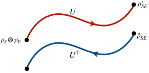
Figure 1: General schematics for the forward and backward trajectories for the fluctuation theorems.

The quantum trajectory is specified by the four measurement outcomes $\gamma=\{n,\nu,m,\mu\}$, which occurs with path probability

$$P_{F}[\gamma]=|\langle\psi_{m},\phi_{\mu}|U|n,\nu\rangle|^{2}p_{n}q_{\nu}.$$ (52)

In order to build a fluctuation theorem one must now establish the backward process, corresponding to the time-reverse evolution with unitary $U^{\dagger}$. The key observations of Ref. Manzano2017a, however, is that this backwards process is not unique. The arbitrariness comes from the choice of initial state $\tilde{\rho}_{SE}$ for the backwards evolution (see Fig. 1). Different choices, as we now show, lead to different expressions for the entropy production. This is also intimately related to the notion of Petz recovery map, a systematic way of building reverse processes for general quantum channels, as considered in Kwon2018c.

For the moment, let us leave $\tilde{\rho}_{SE}$ unspecified. We consider a backward process where $\tilde{\rho}_{SE}$ is first measured in the basis $|\psi_{m}\rangle\otimes|\phi_{\mu}\rangle$, then put to evolve with $U^{\dagger}$ and finally measured one more time, now in the basis $|n\rangle\otimes|\nu\rangle$. The corresponding backward trajectory probability will thus be

$$P_{B}[\gamma]=|\langle n,\nu|U^{\dagger}|\psi_{m},\phi_{\mu}\rangle|^{2}\tilde{\rho}_{m\mu},$$ (53)

where $\tilde{\rho}_{m\mu}=\langle\psi_{m},\phi_{\mu}|\tilde{\rho}_{SE}|\psi_{m},\phi_{\mu}\rangle$.

Armed with $P_{F}$ and $P_{B}$, the entropy production is then defined as usual, as Gallavotti1995; Evans1993; Crooks1998:

$$\sigma[\gamma]=\ln\frac{P_{F}[\gamma]}{P_{B}[\gamma]}.$$ (54)

By construction, this quantity satisfies an integral fluctuation theorem, $\langle e^{-\sigma[\gamma]}\rangle=1$. Using Eqs. (52) and (53) the dynamical term cancels out, leaving us only with the boundary term,

$$\sigma[\gamma]=\ln\frac{p_{n}q_{\nu}}{\tilde{\rho}_{m\mu}}.$$ (55)

As we will now discuss, depending on the choice of $\tilde{\rho}_{SE}$, this expression will unravel in different ways.

First, suppose we choose $\tilde{\rho}_{SE}=\rho_{S}^{\prime}\otimes\rho_{E}$. This means the system is taken at the final state (25), whereas the bath is reset to the initial state $\rho_{E}$. In this case $\tilde{\rho}_{m\mu}=p_{m}^{\prime}q_{\mu}$ and Eq. (55) becomes

$$\sigma[\gamma]=\ln\frac{p_{n}q_{\nu}}{p_{m}^{\prime}q_{\mu}}.$$

The average entropy production is computed as $\langle\sigma\rangle=\sum_{\gamma}\sigma[\gamma]P[\gamma]$. Carrying out the sum, one finds

$$\langle\sigma\rangle=\mathcal{I}_{\rho_{SE}^{\prime}}(S\!:\!E)+S(\rho_{E}^{\prime}||\rho_{E})=S\Big{(}\rho_{SE}^{\prime}\;||\;\rho_{S}^{\prime}\otimes\rho_{E}\Big{)},$$ (56)

which is precisely the definition of $\Sigma$ in Eq. (26). Notice how $\langle\sigma\rangle$ is just the relative entropy between the final state $\rho_{SE}^{\prime}$ of the forward process and the initial state $\rho_{S}^{\prime}\otimes\rho_{E}$ of the backwards process. This provides a solid physical basis for this expression, as being related to the act of tracing over the environment: The two terms in Eq. (56) appear because we reset $E$ in the backward process, meaning we lost all access to both the correlations developed between $S$ and $E$, as well as the changes that were made in the state of $E$.

As a second choice, suppose $\tilde{\rho}_{SE}=\rho_{S}^{\prime}\otimes\rho_{E}^{\prime}$. That is, $S$ and $E$ are initialized in the backward process at the final states of the forward process, but marginalized to destroy any correlations between them. Arguably, correlations are the most difficult part to access, since they require global operations on $S$+$E$. In this case Eq. (55) becomes $\sigma[\gamma]=\ln(p_{n}q_{\nu})/(p_{m}^{\prime}q_{\mu}^{\prime})$ which, upon averaging, yields

$$\langle\sigma\rangle=\mathcal{I}_{\rho_{SE}^{\prime}}(S\!:\!E)=\Delta S_{S}+\Delta S_{E}.$$ (57)

Hence, irreversibility stems solely from the $SE$ correlations that are no longer accessible.

As a third choice, one may take the post-measurement state rCl ~ρ_SE = Δ(ρ_SE’) &:= ∑_mμ —ψ_m,ϕ_μ⟩⟨ψ_m,ϕ_μ— ρ_SE’ — ψ_m,ϕ_μ⟩⟨ψ_m,ϕ_μ—
= ∑_m,μ ρ_mμ’ —ψ_m⟩⟨ψ_m— ⊗— ϕ_μ⟩⟨ϕ_μ—, which is obtained from the final state $\rho_{SE}^{\prime}$ after measuring in the $|\psi_{m}\rangle\otimes|\phi_{\mu}\rangle$ basis. Thus, it corresponds to the maximally dephased state in the basis $|\psi_{m},\phi_{\mu}\rangle$ (note that albeit dephased, this state is still classically correlated). The entropy production (55), upon averaging, reduces in this case to

$$\langle\sigma\rangle=S(\Delta(\rho_{SE}^{\prime}))-S(\rho_{SE}^{\prime})=\mathcal{C}(\rho_{SE}^{\prime}),$$ (58)

which is the relative entropy of coherence Streltsov2016a. We thus conclude that, for this choice of backward protocol, the irreversibility stems solely from the decoherence of the measurement backaction in the final basis $|\psi_{m},\phi_{\mu}\rangle$.

In order to perform a final measurement with absolutely no backaction, one would have to measure $S+E$ in the global basis diagonalizing $\rho_{SE}^{\prime}$. In this case the entropy production would, on average, be identically zero and the process is reversible. However, this requires assessing fully non-local degrees of freedom of $S$ and $E$, which quickly becomes prohibitive even for small quantum systems.

As a final choice of measurement, we can assume that both system and environment are completely reset, so $\tilde{\rho}_{SE}=\rho_{S}\otimes\rho_{E}$ is exactly the initial state. Eq. (55) then becomes $\sigma=\ln(p_{n}q_{\nu})/(p_{m}q_{\mu})$ which, upon averaging, becomes rCl ⟨σ⟩&= I_ρ_SE’(S​ : ​ E) + S(ρ_S’——ρ_S) + S(ρ_E’ —— ρ_E). The first and last terms are exactly the original definition of $\Sigma$ in Eq. (26). However, we now get the additional term $S(\rho_{S}^{\prime}||\rho_{S})$, quantifying how much the system was pushed away from equilibrium. This is a consequence of the fact that in the backward process, we also reset the system to its original thermal state, thus introducing an additional degree of irreversibility.

In the particular case where both system and environment start in thermal states, but at different temperatures, $\rho_{S}=e^{-\beta_{S}H_{S}}/Z_{S}$ and $\rho_{E}=e^{-\beta_{E}H_{E}}/{Z_{E}}$, Eq. (III.5) reduces to

$$\langle\sigma\rangle=\beta_{S}\Delta H_{S}+\beta_{E}\Delta H_{E},$$ (59)

where $\Delta H_{S(E)}$ are the changes in energy in the system and environment respectively. This choice of $\tilde{\rho}_{SE}$ therefore corresponds to the famous exchange fluctuation theorem Jarzynski2004a. If, on top of all this, the unitary satisfies strict energy conservation [Eq. (46)], then we may define $Q_{E}:=\Delta H_{E}=-\Delta H_{S}$, in which case the entropy production reduces to

$$\langle\sigma\rangle=(\beta_{E}-\beta_{S})Q_{E},$$ (60)

which is the expression appearing in Jarzynski2004a.

A summary of these results is presented in Table 1. The main message from this Section is that the definition of entropy production is actually not unique, but depends on the assumptions about which aspects of the system-environment dynamics become inaccessible or irretrievable. The definition (26), which we have focused on most of this Section, contemplates the most general scenario where everything pertaining to the environment is assumed to be lost after the interaction. If the environment is macroscopic, highly chaotic and etc. (e.g. a bucket of water), this will inevitably be the case, so that Eq. (26) becomes the only relevant definition of entropy production. But in the quantum domain, comparing the different definitions may be quite relevant.

One may also attempt to compare the relative importance of each term in these expressions. Let us assume that the bath is much larger than the system so that the process only pushes it slightly away from equilibrium. That is, such that $\rho_{E}^{\prime}=\rho_{E}+\mathcal{O}(\epsilon)$, for some small parameter $\epsilon$. Using standard perturbation theory one then finds that $\Delta S_{E}\propto\epsilon$ while $S(\rho_{E}^{\prime}||\rho_{E})\propto\epsilon^{2}$ Rodrigues2019. Thus, it becomes irrelevant whether to include or not the relative entropy term, since the mutual information tends to dominate. This, however, is not always the case, as recently elucidated in  Ptaszynski2019b. As the authors discuss, the mutual information is actually bounded by the Araki-Lieb inequality,

$$\mathcal{I}_{\rho_{SE}^{\prime}}(S\!:\!E)\leqslant 2\text{min}\big{\{}S(\rho_{S}^{\prime}),S(\rho_{E}^{\prime})\big{\}}.$$

For small $S$ and large $E$, $\mathcal{I}$ will be essentially capped by $S(\rho_{S}^{\prime})$. On the other hand, the relative entropy $S(\rho_{E}^{\prime}||\rho_{E})$ is unbounded and can thus increase indefinitely over time. This will be the case, for instance, in non-equilibrium steady-states of systems connected to multiple baths.

The above discussion can also be extended to multiple measurements. One way to accomplish this is through a collisional model approach, as will be discussed in Sec. V.1. This will simply lead to a composition of the results presented in this section. Alternatively, one may also analyze it from the perspective of stochastic master equations, describing continuously measured systems. This was done in Horowitz2013a; Horowitz2014 and yields the entropy production as a function of the entire trajectory of quantum jumps. The exploration of different choices for the reverse trajectory, however, is not discussed as the framework is based solely on the reduced description of the system, in terms of a master equation. However, at the ensemble level, the authors obtain an entropy production consistent with Eq. (48), which should thus correspond to the bath reset choice (first line in Table 1).

Table 1: Different choices for the initial state $\tilde{\rho}_{SE}$ of the backward process and the corresponding formula for the average entropy production $\langle\sigma\rangle$.

$\tilde{\rho}_{SE}$	$\langle\sigma\rangle$
$\rho_{S}^{\prime}\otimes\rho_{E}$	$\mathcal{I}_{\rho_{SE}^{\prime}}(S\!:\!E)+S(\rho_{E}^{\prime}||\rho_{E})\equiv\Sigma$
(bath reset)	(Eq. (26))
$\rho_{S}^{\prime}\otimes\rho_{E}^{\prime}$	$\mathcal{I}_{\rho_{SE}^{\prime}}(S\!:\!E)$
(correlations destroyed)	$\big{(}=\Delta S_{S}+\Delta S_{E}\big{)}$
$\Delta(\rho_{SE}^{\prime})$	$C(\rho_{SE}^{\prime})$
(post-measurement state)	(relative entropy of coherence)
$\rho_{S}\otimes\rho_{E}$	$\mathcal{I}_{\rho_{SE}^{\prime}}(S\!:\!E)+S(\rho_{S}^{\prime}||\rho_{S})+S(\rho_{E}^{\prime}||\rho_{E})$
	$=(\beta_{S}-\beta_{E})Q_{E}$
(both reset)	Jarzynski2004a

III.6 Non-equilibrium lag

Figure 2: The typical non-equilibrium lag scenario. A system initially prepared in a thermal state $\rho_{i}^{\text{th}}$ is driven unitarily by a work protocol to a non-equilibrium state $\rho^{\prime}$. After the protocol, the system is allowed to thermalize from $\rho^{\prime}$ to $\rho_{f}$.

A scenario which is deeply related to the above, and which has been the subject of considerable research, is the non-equilibrium lag that occurs when an isolated quantum system undergoes a work protocol. This has been covered in detail in Campisi2011. Here we focus only on the most recent developments.

We consider a system $S$ initially prepared in the equilibrium state $\rho_{i}^{\text{th}}=e^{-\beta H_{i}}/Z_{i}$, at temperature $\beta$ and Hamiltonian $H_{i}$. The system is then driven by a work protocol $\lambda(t)$ which changes the Hamiltonian from $H_{i}=H(\lambda(0))$ to $H_{f}=H(\lambda(\tau))$, where $\tau$ is the duration of the protocol. The drive causes the system to evolve unitarily to a non-equilibrium state $\rho^{\prime}=V\rho_{i}^{\text{th}}V^{\dagger}$, where $V$ is the time-evolution operator generated by $H(\lambda(t))$. After the protocol is applied, the system is then placed in contact with a bath and allowed to fully thermalize towards a new equilibrium state $\rho_{f}^{\text{th}}=e^{-\beta H_{f}}/Z_{f}$ (see Fig. 2).

The unitary drive produces no entropy since the dynamics is closed. Irreversibility stems solely from the thermalization step. The entropy production for this relaxation process will be given, in the simplest scenario, by Eq. (48). Since the thermalization is total, the second term vanishes, leaving us with

$$\Sigma=S(\rho^{\prime}||\rho_{f}^{\text{th}}),$$ (61)

Despite being associated to the thermalization process, it turns out this quantity is also of significance to the unitary evolution in itself. In fact, usually this is defined without even mentioning the thermalization. The reason is that Eq. (61) is also directly associated with the irreversible work produced by the unitary $V$:

$$\Sigma\equiv\beta W_{\text{irr}}=\beta(\langle W\rangle-\Delta F),$$ (62)

where $\langle W\rangle=\operatorname{tr}(H_{f}\rho^{\prime})-\operatorname{tr}(H_{i}\rho_{i}^{\text{th}})$ is the average work and $\Delta F=-T\ln Z_{f}/Z_{i}$ is the change in equilibrium free energy. For this reason, Eq. (61) is also called the non-equilibrium lag. For all intents and purposes, “non-equilibrium lag” can be taken as a synonym of entropy production. The reason to introduce this terminology is simply to emphasize that it refers to the unitary protocol, for which no entropy is produced. In the past years, significant attention has been given to the non-equilibrium lag, particularly in the context of quantum phase transitions. These will be reviewed in Sec. LABEL:sec:inf_quenches.

The non-equilibrium lag can also be studied from a stochastic perspective, using the two-point measurement scheme; the first measurement is done in the eigenbasis $|n_{i}\rangle$ of $H_{i}$ and the second in the eigenbasis $|m_{f}\rangle$ of $H_{f}$. The stochastic entropy production associated to this process is then Campisi2011

$$\sigma[n_{i},m_{f}]=\ln p_{n_{i}}^{\text{th}}/p_{m_{f}}^{\text{th}}=\beta(E_{m_{f}}^{f}-E_{n_{i}}^{i}-\Delta F),$$ (63)

where $E^{i(f)}$ are the energies of $H_{i(f)}$ and $\Delta F=F_{f}-F_{i}=-T\ln Z_{f}/Z_{i}$ is the change in non-equilibrium free energy. Moreover, $p_{n_{i}}^{\text{th}}=e^{-\beta E_{n_{i}}^{i}}/Z_{i}$ is the initial thermal probability and $p_{m_{f}}^{\text{th}}=e^{-\beta E_{m_{f}}^{f}}/Z_{f}$ is a thermal probability associated with the final Hamiltonian $H_{f}$. The probability distribution of $\sigma$ is thus

$$P(\sigma)=\sum\limits_{n_{i},m_{f}}p(m_{f}|n_{i})p_{n_{i}}\delta\bigg{(}\sigma-\sigma[n_{i},m_{f}]\bigg{)},$$ (64)

where $p(m_{f}|n_{i})=|\langle m_{f}|V|n_{i}\rangle|^{2}$ is the transition probability from $|n_{i}\rangle\to|m_{f}\rangle$. By construction, this is such that $\langle\sigma\rangle=\Sigma$ [Eq. (61)].

It is convenient to study the cumulant generating function $K(\lambda)=\ln\langle e^{-\lambda\sigma}\rangle$, which can be conveniently written as Talkner2007; Esposito2009

$$K(\lambda)=\ln\operatorname{tr}\bigg{\{}V^{\dagger}e^{-\beta\lambda(H_{f}-F_{f})}Ve^{\beta\lambda(H_{i}-F_{i})}\rho_{i}^{\text{th}}\bigg{\}}.$$ (65)

The cumulants may be computed from $K(\lambda)$ through the relation

$$\kappa_{n}(\sigma)=(-1)^{n}\frac{\partial^{n}K}{\partial\lambda^{n}}\bigg{|}_{\lambda=0}.$$ (66)

The first cumulant is the average and is given by Eq. (61). Similarly, the second cumulant is the variance and can be written as

$$\text{var}(\sigma)=\operatorname{tr}\big{\{}\rho^{\prime}(\ln\rho^{\prime}-\ln\rho_{f}^{\text{th}})^{2}\big{\}}-S(\rho^{\prime}||\rho_{f}^{\text{th}})^{2},$$ (67)

which is sometimes called the relative entropy variance.

The CGF (65) can also be expressed in terms of the so-called Rényi divergences, which will be discussed further in Sec. LABEL:sec:thermal_ops and are defined as

$$S_{\lambda}(\rho||\sigma)=\frac{1}{\lambda-1}\ln\operatorname{tr}\big{\{}\rho^{\lambda}\sigma^{1-\lambda}\big{\}}$$ (68)

They correspond to a generalization of the relative entropy (28), which is recovered from $S_{\lambda}(\rho||\sigma)$ in the limit $\lambda\to 1$. Comparing (68) with Eq. (65) one then sees that Guarnieri2019:

$$K(\lambda)=(\lambda-1)S_{\lambda}(\rho_{f}^{\text{th}}||\rho^{\prime}),$$ (69)

This expression has been used in several recent studies. Following Guarnieri2018, we will review in Sec. LABEL:sec:resource_reconciliation how (69) can be used as a connection to the resource-theoretic formulation of thermodynamics, which is the subject to Sec. LABEL:sec:thermal_ops. In Sec. LABEL:sec:inf_quenches we review Refs. Miller2019; Scandi2019, which use (69) as a tool to extract the contribution from quantum coherence in slow processes.

IV Information-theoretic aspects

IV.1 Corrections to Landauer’s principle

Landauer’s principle was introduced in Sec. II.3 and is based on the idea that information erasure is an irreversible process, with a fundamental heat cost associated to it. This is synthesized by Eq. (17), representing a lower bound on the heat $Q_{E}$ dissipated to the environment, in terms of the change in entropy $\Delta S_{S}$ of the system. Being a lower bound, one can then conclude that changes in entropy must be accompanied by a fundamental heat cost.

In Sec. II.3 we hinted at the subtle nature of Landauer’s principle: in classical thermodynamics, Eq. (17) is a direct consequence of the 2nd law, but with $S_{S}$ being the thermodynamic entropy of the system. Landauer’s original bound, on the other hand, concerns the information theoretic entropy. The framework put forth in Sec. III, however, unifies both views, as it reformulates the 2nd law in terms of the system’s von Neumann entropy. Indeed, Eqs. (26) and (34) imply that:

$$\Sigma=\mathcal{I}_{\rho_{SE}^{\prime}}(S\!:\!E)+S(\rho_{E}^{\prime}||\rho_{E})=\Delta S_{S}+\beta Q_{E}.$$ (70)

The 2nd law $\Sigma\geqslant 0$ then yields $Q_{E}\geqslant-T\Delta S_{S}$, which is precisely Landauer’s bound (17). Equality is achieved when $\Sigma=0$; i.e., for reversible processes. These results are present already in Esposito2010a, but the link with Landauer’s principle was strengthened in in Reeb2014, a publication which greatly popularized this subject.

Eq. (17) is important because it is universal. The only hypothesis is that the bath is initially thermal (and uncorrelated from the system). Other than that, the bath may have arbitrary dimension and arbitrary Hamiltonian; the system may be prepared in any initial state; and the interaction $U$ can be any unitary whatsoever.

This universality, however, has the downside that, the bound is in general quite loose. Tighter bounds can be obtained by assuming additional information about the environment and/or the process. We now discuss several such formulations, taking care to properly state which additional pieces of information are assumed in each case. First, we consider the case where the only additional piece of information one has is that the environment is finite dimensional, with a Hilbert space dimension $d_{E}$. In this case, when $\Delta S_{S}<0$, the following correction to (17) holds Reeb2014:

$$Q_{E}\geqslant-T\Delta S_{S}+\frac{2T(\Delta S_{S})^{2}}{4+\ln^{2}(d_{E}-1)}.$$ (71)

This shows that finite dimensions impose more strict constraints on heat dissipation. The correction vanishes when $d_{E}\to\infty$; however, notice that the dependence is logarithmic and therefore extremely slow. Additional finite-size bounds are also presented in Reeb2014, although they depend on more complicated functions.

The original bound (17), or its finite size correction (71) become trivial in the limit $T\to 0$. This is clearly unsatisfactory: can erasure really be performed with zero dissipation when $T\to 0$? The bound trivializes in this case due to the term $S(\rho_{E}^{\prime}||\rho_{E})$ in Eq. (70), which diverges when $T\to 0$. To bypass this difficulty, in Timpanaro2019a it was shown how to derive a tighter bound starting only from the mutual information term $\mathcal{I}_{\rho_{SE}^{\prime}}(S\!:\!E)$. The bound in this case acquires the form

$$Q_{E}\geqslant\mathcal{Q}(\mathcal{S}^{-1}(-\Delta S_{S})),$$ (72)

where the functions $\mathcal{Q}(T^{\prime})$ and $\mathcal{S}(T^{\prime})$ are defined as

$$\mathcal{Q}(T^{\prime})=\int\limits_{T}^{T^{\prime}}C_{E}(\tau)d\tau,\qquad\mathcal{S}(T^{\prime})=\int\limits_{T}^{T^{\prime}}\frac{C_{E}(\tau)}{\tau}d\tau,$$ (73)

with $C_{E}(T)$ being the equilibrium heat capacity of the environment. In these expressions $T$ is the actual initial temperature of the environment, whereas $T^{\prime}$ is merely the argument of the functions. This bound requires only one additional piece of information; namely the environment’s heat capacity $C_{E}(T)$. This is to be compared with (17), which requires only a single number, $T$, or with Eq. (71), which requires two numbers, $T$ and $d_{E}$. Admittedly, knowing an entire function $C_{E}(T)$ is definitely more difficult, although the heat capacity is in general an easy quantity to measure experimentally, even at extremely low temperatures. However, one can also show that the bound is always tighter than both (17) and (71). To provide an example, if we happen to have $C_{E}=aT$, for some constant $a$, Eq. (72) becomes

$$Q_{E}\geqslant-T\Delta S_{S}+\frac{\Delta S_{S}^{2}}{2a}.$$ (74)

As in (71), the correction also involves a term proportional to $\Delta S_{S}^{2}$, but with a coefficient that is temperature independent. Thus, in the limit $T\to 0$ the last term still survives, showing that a fundamental heat cost still exists even when $T=0$.

Tighter bounds can also be derived when information about the $SE$ unitary $U$ and the system initial state $\rho_{S}$ are available Goold2014b; Lorenzo2015; Guarnieri2017. Here we review the approach in Goold2014b, which derives a bound using the fluctuating properties of heat. The key idea is to interpret the global map (24) as a quantum channel for the environment, instead of the system, as described by the Kraus map

$$\rho^{\prime}_{E}={{\rm Tr}}_{S}[U(\rho_{S}\otimes\rho_{E})U^{\dagger}]=\sum_{l}A_{l}\,\rho_{E}\,A_{l}^{\dagger},$$ (75)

where $A_{l=jk}=\sqrt{\lambda_{j}}\langle{s_{k}}|{U}|{s_{j}}\rangle$, with $\{\lambda_{j}\}$ and $\{|s_{j}\rangle\}$ being the eigenvalues and eigenstates of $\rho_{S}$. Trace-preservation implies $\sum_{l}A^{\dagger}_{l}A_{l}=\openone_{E}$. Letting $E_{n}$ and $|r_{n}\rangle$ denote the eigenvalues and eigenvectors of $H_{E}$, the heat distribution of the environment (via a two-point measurement) can now be written as Talkner2009.

$$P(Q_{E})=\sum_{l,m,n}\langle{r_{n}}|{A_{l}}|{r_{m}}\rangle(\rho_{E})_{mm}\langle{r_{m}}|{A^{\dagger}_{l}}|{r_{n}}\rangle\delta(Q_{E}-(E_{n}-E_{m}))$$ (76)

with $(\rho_{E})_{nm}=\langle r_{n}|\rho_{E}|r_{m}\rangle$. From this one may now show that $\langle e^{-\beta Q}\rangle={\rm Tr}[\mathbf{M}\,\rho_{S}]$, where $\mathbf{M}={\rm Tr}_{E}[U^{\dagger}\,(\openone_{S}\otimes\rho_{E})\,U]$. Using Jensen’s inequality then leads to

$$\langle Q_{E}\rangle\geqslant-T\ln({\rm Tr}[\mathbf{M}\,\rho_{S}]).$$ (77)

This result establishes a bound on $\langle Q_{E}\rangle$, which depends on both the state of the system as well as the unitary $U$. It therefore naturally encompass also a dependence on the size of $E$, in line with Eq. (71).

Using the formalism of full counting statistics Esposito2009, one can also extend these results to obtain an entire single-parameter family of bounds Guarnieri2017. We first introduce the cumulant generating function of $P(Q_{E})$,

$$\Theta(\eta,\beta)\equiv\ln\left\langle e^{-\eta Q_{E}}\right\rangle=\ln\int P(Q_{E})e^{-\eta Q_{E}}dQ_{E}.$$ (78)

Hölder’s inequality then implies that for $\eta>0$,

$$\beta\langle Q_{E}\rangle\geqslant-\frac{\beta}{\eta}\Theta(\eta,\beta)\quad(\eta>0),$$ (79)

which contains Eq. (77) as a particular case. Conversely, for $\eta<0$ we obtain the upper bounds $\beta\langle Q_{E}\rangle\leqslant\beta\Theta(\eta,\beta)/|\eta|$. In the limit $|\eta|\to 0$ both bounds coincide with $\beta\langle Q_{E}\rangle$.

IV.2 Conditional entropy production

We consider once again the general map (24) of Sec. III. But now we suppose that after the map we measure the environment, or at least a part of it. Funo2013 studied how the information acquired from this measurement affects the entropy production. Since it is only the bath that is measured, there can be no backaction to the system, as this would violate no-signaling. As a consequence, one expects that learning the outcomes of the measurements should always make the the process more reversible; that, is part of the ignorance captured by the entropy production should be resolved.

To formalize this idea, we consider a generalized measurement on $E$ described by Kraus operators $\{M_{k}\}$ and labeled by a set of outcomes $k$. We denote the local states of $S$ and $E$ after the map, conditioned on an outcome $k$, by

$$\rho_{E|k}^{\prime}=\frac{M_{k}\rho_{E}^{\prime}M_{k}^{\dagger}}{p_{k}},\qquad\rho_{S|k}^{\prime}=\frac{1}{p_{k}}\operatorname{tr}_{E}\big{(}M_{k}\rho_{SE}^{\prime}M_{k}^{\dagger}\big{)},$$ (80)

where $p_{k}=\operatorname{tr}(M_{k}\rho_{E}^{\prime}M_{k}^{\dagger})$ is the probability of outcome $k$ (as before, primed quantities always refer to states after the map). One may also verify that $\sum_{k}p_{k}\rho_{S|k}^{\prime}=\rho_{S}^{\prime}$, thus confirming that the measurement in $E$ causes no backaction in $S$. But there may, of course, be a backaction in $E$ so $\tilde{\rho}_{E}:=\sum_{k}p_{k}\rho_{E|k}^{\prime}\neq\rho_{E}^{\prime}$.

We now ask how to construct the entropy production conditioned on a given outcome. The goal is to define, in analogy with Eq. (30), a conditional entropy production $\Sigma_{k}$ and a conditional flux $\Phi_{k}$, which are related by

$$\Sigma_{k}=S(\rho_{S|k}^{\prime})-S(\rho_{S})+\Phi_{k}.$$ (81)

This is still merely a definition, and will only acquire meaning once $\Sigma_{k}$ and $\Phi_{k}$ are defined. Averaging over all outcomes $k$ then yields a relation between the conditional average entropy production and flux:

$$\Sigma_{c}=\sum\limits_{k}p_{k}S(\rho_{S|k}^{\prime})-S(\rho_{S})+\Phi_{c},$$ (82)

where $\Sigma_{c}=\sum_{k}p_{k}\Sigma_{k}$ and similarly for $\Phi_{c}$. The entropy difference on the first two terms of the right-hand side is known as the Ozawa-Groenewold quantum-classical information Groenewold1971; Ozawa1986; Funo2018. Notice also that $\Sigma_{k}$ and $\Phi_{k}$ are not necessarily linear functions of $\rho_{SE}^{\prime}$, so that, in general, their averages $\Sigma_{c}$ and $\Phi_{c}$ do not have to coincide with the unconditional quantities $\Sigma$ and $\Phi$.

Eq. (81) is merely a definition of $\Sigma_{k}$ and $\Phi_{k}$. The relevant question is how to properly define these quantities in a way that is physically consistent. We first analyze the flux. A look at Eq. (33) shows that a natural generalization to the case of conditional states is $\Phi_{k}=S(\rho_{E|k}^{\prime})-S(\rho_{E})+S(\rho_{E|k}^{\prime}||\rho_{E})$, which therefore simply amounts to replacing $\rho_{E}^{\prime}$ with $\rho_{E|k}^{\prime}$. Averaging over all $p_{k}$ and using the second line in Eq. (33), one then finds

$$\Phi_{c}:=\sum\limits_{k}p_{k}\Phi_{k}=\operatorname{tr}\big{\{}(\rho_{E}-\tilde{\rho}_{E})\ln\rho_{E}\big{\}},$$ (83)

where $\tilde{\rho}_{E}=\sum_{k}p_{k}\rho_{E|k}^{\prime}$. If the measurement is performed on the initial eigenbasis of $\rho_{E}$, it then follows that $\Phi_{c}=\Phi$ (even though $\tilde{\rho}_{E}\neq\rho_{E}^{\prime}$). This result has a clear and beautiful physical interpretation: the entropy flux refers only to the flow of information to the environment. It should therefore be independent on whether or not we condition on any measurement outcomes. The flux should therefore only change if there is backaction from the measurement. In other words, the difference $\Phi_{c}-\Phi$ has nothing to do with the system nor the $SE$ interaction, but only with the backaction caused by the measurement. For this reason, we henceforth assume that the measurement is such that $\Phi_{c}=\Phi$. Interestingly, this assumption has also been used implicitly in Ref Breuer2003, which defines entropy production from the perspective of quantum jump trajectories.

Using $\Phi_{c}=\Phi$ in Eq. (82) and comparing with Eq. (30) allows one to conclude that

$$\Sigma_{c}=\Sigma-\chi_{M}(\rho_{S}^{\prime}),$$ (84)

where rCl χ_M(ρ_S’) &= S(ρ_S’) - ∑_k p_k S(ρ_S—k’)=∑_k p_k S(ρ_S—k’ —— ρ_S’), is the Holevo quantity Nielsen, which is always non-negative. Eq. (84) beautifully illustrates the idea of reducing irreversibility through measurement: Conditioning on the measurement outcomes reduces, on average, the entropy production by an amount proportional to the Holevo quantity, an object with numerous applications in information theory.

The Holevo quantity $\chi_{M}$ is a basis-dependent version of the classical information used in quantum discord theory Modi2012. It thus follows that, for any choice of measurement operators $\{M_{k}\}$, one should have $\chi_{M}(\rho_{S}^{\prime})\leqslant I_{\rho_{SE}^{\prime}}(S\!:\!E)$. Comparing with the definition of $\Sigma$ in Eq. (26), one then concludes from Eq. (84) that

$$\Sigma_{c}=I_{\rho_{SE}^{\prime}}(S\!:\!E)+S(\rho_{E}^{\prime}||\rho_{E})-\chi(\rho_{S}^{\prime})\geqslant S(\rho_{E}^{\prime}||\rho_{E}).$$

Hence, even though $\Sigma_{c}\leqslant\Sigma$, it is nonetheless still strictly non-negative. This occurs because the interaction irreversibly pushes the bath away from equilibrium, so that even if all possible information was to be acquired, the dynamics would still be irreversible.

IV.3 Heat flow in the presence of correlations

Another key manifestation of information in thermodynamics is the influence of initial correlations in the heat flow between two bodies. According to the second law, if we put in contact two systems $A$ and $B$, initially prepared in equilibrium at different temperatures, heat will always flow hot to cold [Eq. (11)]. This assumes, however, that the two bodies are initially uncorrelated. If that is not true, heat may eventually flow from cold to hot. This problem was first considered in the quantum scenario in Partovi2008, who discussed only the case where the global state of $AB$ is pure. This was then generalized in Refs. Jennings2010 and Bera2017b, who also addressed some of the information-theoretical aspects of the problem. An experimental demonstration of this effect was recently performed in a nuclear magnetic resonance setup Micadei2017. In a broader sense, these ideas are ultimately related to the use of mutual information to reduce entropy, as first discussed in the seminal paper by Lloyd1989.

We consider two systems with Hamiltonians $H_{A}$ and $H_{B}$, prepared in a global (generally correlated) state $\rho_{AB}$. We assume, however, that the reduced density matrices of $A$ and $B$ are still thermal, $\rho_{A}=\operatorname{tr}_{B}\rho_{AB}=e^{-\beta_{A}H_{A}}/Z_{A}$, and $\rho_{B}=e^{-\beta_{B}H_{B}}/Z_{B}$, at different temperatures $\beta_{A}$ and $\beta_{B}$. The two systems are then put to interact with a unitary $U$ satisfying strict energy conservation $[U,H_{A}+H_{B}]=0$ (cf. Eq. (46)). The state after the interaction is thus $\rho_{AB}^{\prime}=U\rho_{AB}U^{\dagger}$, from which one can compute the corresponding marginals $\rho_{A}^{\prime}$ and $\rho_{B}^{\prime}$.

The correlations between $A$ and $B$ are characterized by the mutual information $\mathcal{I}_{\rho_{AB}}(A\!:\!B)$ defined in Eq. (27). Since the dynamics is unitary it follows that $S(\rho_{AB}^{\prime})=S(\rho_{AB})$, which allows one to show that

$$\Delta I(A\!:\!B)=\Delta S_{A}+\Delta S_{B},$$ (85)

where $\Delta I(A\!:\!B)=I_{\rho_{AB}^{\prime}}(A\!:\!B)-I_{\rho_{AB}}(A\!:\!B)$ is the change in the mutual information between $A$ and $B$.

Next, consider the quantity

$$\mathcal{S}=S(\rho_{A}^{\prime}||\rho_{A})+S(\rho_{B}^{\prime}||\rho_{B})\geqslant 0,$$ (86)

which is non-negative because the relative entropies are non-negative. This quantity is a part of the entropy production, when cast in terms of the Jarzynski-Wójcik scenario [cf. Eq. (III.5)]. What is important for the present purposes is that this quantity is purely local, depending only on the reduced density matrices of $A$ and $B$ before and after the interaction. Substituting the initial thermal forms of $\rho_{A}$ and $\rho_{B}$, together with Eq. (85), then leads to Jennings2010:

$$\mathcal{S}=\beta_{A}\Delta H_{A}+\beta_{B}\Delta H_{B}-\Delta I(A\!:\!B)\geqslant 0.$$ (87)

Let us assume $T_{A}>T_{B}$. Due to strict energy conservation, the average heat exchanged is simply defined as

$$Q_{B}=\Delta H_{B}=\operatorname{tr}\big{\{}H_{B}(U\rho_{AB}U^{\dagger}-\rho_{AB})\big{\}}=-\Delta H_{A},$$ (88)

so that Eq. (87) becomes

$$(\beta_{B}-\beta_{A})Q_{B}\geqslant\Delta I(A\!:\!B).$$ (89)

This can be viewed as a generalization of the bound (11) to take into account initial correlations.

If $A$ and $B$ are initially uncorrelated then $\Delta I(A\!:\!B)=I_{\rho_{AB}^{\prime}}(A\!:\!B)\geqslant 0$, which implies $Q_{B}$ must have the same sign as $\beta_{B}-\beta_{A}$ (i.e., heat flows from hot to cold). But if they are initially correlated and the process is such that this correlation is consumed ($\Delta I(A\!:\!B)<0$), then it is possible for heat to flow from cold to hot. This is thus an example of a situation where an information theoretic resource is being consumed to perform a thermodynamic task that would not naturally occur. This is akin to refrigerators, where heat also flows from cold to hot, but the resource being used is work from the electrical plug. The result can also be formulated in the language of Maxwell’s Demons. A demon, in this context, has access to additional information, in the form of global correlations shared between $A$ and $B$. These correlations can then be consumed as a thermodynamic resource.

Correlations, of course, will not always make heat flow from cold to hot. They may very well have the opposite effect, accelerating the heat from hot to cold. An illustrative example is the problem studied experimentally in Micadei2017. Consider two qubits with $H_{i}=\Omega|e\rangle\langle e|_{i}$ ($i=A,B$) and initially prepared in a correlated state of the form

$$\rho_{AB}=\rho_{A}^{\text{th}}\otimes\rho_{B}^{\text{th}}+\chi$$ (90)

where $\rho_{i}^{\text{th}}=(1-f_{i})|g\rangle\langle g|+f_{i}|e\rangle\langle e|$, with $f_{i}=(e^{\Omega/T_{i}}+1)^{-1}$, are the local thermal states of each qubit and $\chi=\alpha e^{i\theta}|g,e\rangle\langle e,g|+\alpha e^{-i\theta}|e,g\rangle\langle g,e|$ represents the correlations, with $\alpha$ and $\theta$ being real parameters. The two qubits are then put to interact with an energy-preserving unitary $U=\exp\big{\{}-igt(e^{i\phi}|g,e\rangle\langle e,g|+e^{-i\phi}|e,g\rangle\langle g,e|)\big{\}}$, where $\phi$ is an arbitrary phase and $g$ is the interaction strength. The heat $Q_{B}=\Delta H_{B}$ that enters system $B$ at time $t$ will be given by

$$Q_{B}(t)=\Omega\sin(gt)\bigg{[}(f_{A}-f_{B})\sin(gt)-2\alpha\sin(\theta-\phi)\cos(gt)\bigg{]}.$$ (91)

We again assume $T_{A}>T_{B}$ for concreteness. Since $f_{i}$ is monotonically increasing with $T_{i}$, when $\alpha=0$ we always get $Q_{B}\propto(f_{A}-f_{B})>0$, so that heat will flow from hot to cold. But when $\alpha\neq 0$, the direction of the heat flow will actually depend on a fine interplay between the phases $\theta$ and $\phi$ appearing in $\chi$ and $U$, respectively. These phases may combine either constructively, reversing the heat flow, or destructively, accelerating the already natural flow direction.

IV.4 Fluctuation theorem under classical and quantum correlations

The problem treated in Sec. IV.3 can also be analyzed from a quantum trajectories perspective, which will serve to highlight the non-trivial role of quantum vs. classical correlations. We begin by considering the case of two-point measurements (TPM), where both $A$ and $B$ are measured at the beginning and the end of the process. Jevtic2015a discusses the implications of measuring in the local energy bases $|n_{A}\rangle$ and $|n_{B}\rangle$ of the Hamiltonians $H_{A}$ and $H_{B}$. A quantum trajectory will be specified by four quantum numbers, $\gamma=(n_{A},n_{B},m_{A},m_{B})$ and occurs with probability

$$\mathcal{P}[\gamma]=|\langle m_{A}m_{B}|U|n_{A}n_{B}\rangle|^{2}p_{n_{A}n_{B}},$$ (92)

where $p_{n_{A}n_{B}}=\langle n_{A}n_{B}|\rho_{AB}|n_{A}n_{B}\rangle$. Crucially, since $\rho_{AB}$ is not a product state, in general $p_{n_{A}n_{B}}\neq p_{n_{A}}p_{n_{B}}$.

The probability that a heat $q_{B}[\gamma]=E_{m_{B}}-E_{n_{B}}$ enters system $B$ will then be given by $P(q_{B})=\sum_{\gamma}\delta(q_{B}-q_{B}[\gamma])\;\mathcal{P}[\gamma]$. Using this to compute the average heat $\langle q_{B}\rangle$, we find

$$\langle q_{B}\rangle=\operatorname{tr}\big{\{}H_{B}\big{[}U\Delta(\rho_{AB})U^{\dagger}-\Delta(\rho_{AB})\big{]}\big{\}},$$ (93)

where $\Delta(\rho_{AB})=\sum_{n_{A},n_{B}}|n_{A}n_{B}\rangle\langle n_{A}n_{B}|\rho_{AB}|n_{A}n_{B}\rangle\langle n_{A}n_{B}|$ is the operation of fully dephasing $\rho_{AB}$ in the basis $|n_{A}n_{B}\rangle$.

The important point to realize now is that Eq. (93) is, in general, different from the average heat in Eq. (88). The difference is due to the presence of the dephasing operator $\Delta$ and is thus a consequence of the measurement backaction, which dephases $\rho_{AB}$. The two quantities will only coincide when $\rho_{AB}$ is already diagonal in $|n_{A}n_{B}\rangle$. Put it differently, when $\rho_{AB}$ is not diagonal, the TPM scheme used here will fundamentally change the amount of heat exchanged between the two systems, producing an entirely different dynamics when compared with the bare unitary evolution. The entropy production is thus extrinsic; that is, dependent not only on the systems $A$ and $B$, but also on the details on how one performs the experiment.

This highlights the fundamental difference between correlations present in the populations (i.e., which are diagonal in $|n_{A}n_{B}\rangle$) and correlations which are present in the coherences (off-diagonals). The latter can be viewed as a basis-dependent quantum discord; i.e., as the amount of discord present in the energy basis (the energy basis appears as a preferred basis due to the energy-conserving nature of the unitary $U$; as will be reviewed in Sec. V.2).

Returning to Eq. (92), let us introduce the reverse process, where both $A$ and $B$ start at the same state, but one applies the unitary $U^{\dagger}$ instead (this is the Jarzynski-Wójcik scenario of Sec. III.5). The probability for the backward trajectory $\gamma^{*}=(m_{A},m_{B},n_{A},n_{B})$ will be given by $\mathcal{P}[\gamma^{*}]=|\langle n_{A}n_{B}|U^{\dagger}|m_{A}m_{B}\rangle|^{2}p_{m_{A}m_{B}}$. The ratio of the two processes reduce to $\mathcal{P}[\gamma]/\mathcal{P}[\gamma^{*}]=p_{n_{A}n_{B}}/p_{m_{A}m_{B}}$, since the dynamical term cancels out (as usual). To make the physics of this ratio more evident, we introduce the stochastic mutual information $I_{n_{A}n_{B}}=\ln p_{n_{A}n_{B}}/p_{n_{A}}p_{n_{B}}$, where $p_{n_{A}}=\sum_{n_{B}}p_{n_{A}n_{B}}$ (and similarly for $p_{n_{B}}$) are the marginal distributions of the initial state, which we chose to be thermal, $p_{n_{A}}=e^{-\beta_{A}E_{n_{A}}}/Z_{A}$. The average of $I_{n_{A}n_{B}}$ over $p_{n_{A}n_{B}}$ yields the mutual information of the dephased state

$$\langle I_{n_{A}n_{B}}\rangle=\sum\limits_{n_{A},n_{B}}p_{n_{A}n_{B}}\ln\frac{p_{n_{A}n_{B}}}{p_{n_{A}}p_{n_{B}}}=\mathcal{I}_{\Delta(\rho_{AB})}(A\!:\!B).$$ (94)

where $\mathcal{I}_{\rho}(A\!:\!B)$ is defined in Eq. (27).

Writing $p_{n_{A}n_{B}}=p_{n_{A}}p_{n_{B}}e^{I_{n_{A}n_{B}}}$ allows us to express $\mathcal{P}[\gamma]/\mathcal{P}[\gamma^{*}]=\big{(}p_{n_{A}}p_{n_{B}}/p_{m_{A}}p_{m_{B}}\big{)}e^{-\Delta I[\gamma]}$, where $\Delta I[\gamma]=I_{m_{A}m_{B}}-I_{n_{A}n_{B}}$. But since the reduced states are thermal, $p_{n_{\alpha}}/p_{m_{\alpha}}=e^{\beta_{\alpha}(E_{m_{\alpha}}-E_{n_{\alpha}})}$, and we may finally write

$$\frac{\mathcal{P}[\gamma]}{\mathcal{P}[\gamma^{*}]}=e^{(\beta_{B}-\beta_{A})q_{B}[\gamma]-\Delta I[\gamma]},$$ (95)

where we also used the fact that $E_{m_{A}}-E_{n_{A}}=-(E_{m_{B}}-E_{n_{B}})$.

Eq. (95) represents a modified exchange fluctuation theorem, generalizing the results of Jarzynski2004a to the case where $A$ and $B$ have initial correlations. Eq. (95) implies a non-equilibrium equality $\langle e^{(\beta_{B}-\beta_{A})q_{B}[\gamma]-\Delta I[\gamma]}\rangle=1$, which yields the bound

$$(\beta_{B}-\beta_{A})\langle q_{B}[\gamma]\rangle\geqslant\langle\Delta I[\gamma]\rangle.$$ (96)

This is structurally similar to Eq. (89). However, as discussed before, they cannot be directly compared since they pertain to different processes due to the dephasing action of the first measurement.

The above results show clearly that, when constructing fluctuation theorems, quantum correlations are fundamentally hampered by the backaction of the two-point measurement scheme. A way to circumvent this is to use the notion of augmented trajectories, first discussed by Dirac Dirac1945 and used more recently in Park2017; Micadei2019. We decompose the initial (correlated) state of $AB$ as $\rho_{AB}=\sum_{s}p_{s}|s\rangle\langle s|$, where $|s\rangle$ are eigenvectors living on the composite Hilbert space of $AB$. Before the dynamics, we perform instead a measurement in the basis $|s\rangle$. The second measurement can be in the energy basis, as in Sec. IV.4, since it does not matter if we destroy the correlations after the end of the protocol.

The quantum trajectory will therefore be described in this case by the quantum numbers $\gamma=(s,m_{A},m_{B})$ and the corresponding path probability will be given, instead of Eq. (92), by $\mathcal{P}[\gamma]=|\langle m_{A}m_{B}|U|s\rangle|^{2}p_{s}$. Knowing the outcome $s$ of the first measurement, however, does not uniquely specify which energy eigenstates $|n_{A}n_{B}\rangle$ the two systems were initially in. In order to account for this, we augment the trajectories by considering the conditional probability $p_{n_{A}n_{B}|s}=|\langle n_{A}n_{B}|s\rangle|^{2}$ that $AB$ are found in $|n_{A}n_{B}\rangle$ given that globally they are in $|s\rangle$. The augmented trajectory $\tilde{\gamma}=(s,n_{A},n_{B},m_{A},m_{B})$ will then have a path probability

$$\tilde{\mathcal{P}}[\tilde{\gamma}]=|\langle m_{A}m_{B}|U|s\rangle|^{2}p_{s}p_{n_{A}n_{B}|s}.$$ (97)

This formulation fixes the issues that arise from the backaction of the first measurement. For instance, as shown in Ref. Micadei2019, it leads to the full identity (89) and not its dephased version (96).

Eq. (97) also illustrates well a recurring problem in extending thermodynamics to the quantum regime. Thermodynamics does not deal with states, but with processes; i.e., with transformations between states. Assessing these transformations therefore touches on the inevitable measurement backaction. Eq. (97) circumvents this by constructing a distribution free from any backaction. This distribution, however, has to be constructed using full state tomography. An alternative approach, put forth in Levy2019, formulates the problem using instead the notion of quasiprobabilities; that is, probabilities which can take on negative values. As the authors show, these negativities are directly related to the notion of contextuality.

V Quantum dynamics and the classical limit

The global unitary map (25) is extremely general and represents the basic structure behind most open system dynamics (the only assumption in it is that $S$ and $E$ are initially uncorrelated). To make it practical, however, this map has to be specialized to specific paradigms. The usual paradigm in open quantum systems Gardiner2004; Breuer2007; Rivas2012 is to assume that the environment is macroscopically large and the unitary is left turned on for an arbitrary time. Eq. (24) is then naturally reinterpreted as the continuous time map

$$\rho_{S}(t)=\mathcal{E}_{t}(\rho_{S}(0))=\operatorname{tr}_{E}\bigg{\{}U(t)\big{(}\rho_{S}(0)\otimes\rho_{E}\big{)}U^{\dagger}(t)\bigg{\}}.$$ (98)

Common questions in the theory of open quantum systems, such as whether or not the map will be divisible, are all contained in the properties of $\rho_{E}$ and $U(t)$.

All results derived in Sec. III for the entropy production remain valid in this case, although it becomes more natural to study the entropy production rate $\dot{\Sigma}=d\Sigma/dt$. An important observation, however, is that even though $\Sigma\geqslant 0$ by construction, this is not in general guaranteed for $\dot{\Sigma}$. This, of course, is expected to happen for macroscopic environments, but has to be analyzed in a case-by-case basis. In fact, temporary negativities in $\dot{\Sigma}(t)$ can be used as a measure of non-Markovianity BreuerRMP; deVega2017, as they represent instances of time where information backflows to the system (which fits well with the interpretation of $\dot{\Sigma}$ as a measure of irreversibility). This will be reviewed in Sec. LABEL:ssec:non_mark.

More serious difficulties may arise, however, when one is interested in quantum master equations derived from the map (98). The problem is that master equations use several approximations to describe the dynamics solely from the optics of the reduced state of the system. They therefore have no information about the global $S+E$ state, which is paramount for quantifying entropy production. Thus, while these approximations may be reasonable for describing the dynamics, they can be disastrous for the thermodynamics. Of course, in many situations no issues arise. And, in fact, master equations are routinely employed in the study of thermodynamics, e.g. in the context of transport. However, there are situations where one may arrive at inconsistencies. For instance, in Ref. Levy2014 it was shown how local master equations seem to violate the second law (allowing, e.g., heat to flow from cold to hot). If one has access also to the global dynamics, this would never happen by construction. This was used in DeChiara2018 to reconcile local master equations with thermodynamics.

The thermodynamics of quantum master equations has to be analyzed in a case-by-case basis. Instead, we have opted to focus in this review on an alternative paradigm of open system, called collisional models (also called “repeated interactions”). These models, to be detailed below, have been used for a long time in different contexts Rau1963; Englert2002; Scarani2002. However, they recently gained a surge in popularity Karevski2009; Giovannetti2012; McCloskey2014; Landi2014b; Barra2015; Lorenzo2015; Strasberg2016; Pezzutto2016; Cusumano2018; Pereira2018, largely because they allow full control over the approximations being employed. We will review the thermodynamics of collisional models, which were laid out on firm grounds in Strasberg2016. Throughout the section, we will also connect them with master equations, following Barra2015; DeChiara2018. In fact, we will discuss how some of the famous results for the thermodynamics of master equations can actually be derived as limiting cases of such models. This includes the famous result by Spohn Spohn1978, as well as the formulation of continuous measurements in Horowitz2013a. We also review how collisional models can be used to see the emergence of a classical limit and the classical rules of stochastic thermodynamics Cwikli2015.

V.1 Collisional models

Collisional models draws inspiration from Boltzmann’s original Stosszahlansatz (molecular chaos hypothesis). The open system dynamics is envisioned as a series of sequential interactions, where in each time interval the system only interacts with a tiny fraction of the environment (which we shall henceforth refer to as an ancilla). After this interaction the ancilla is discarded and a fresh new one is introduced, again prepared in a thermal state. This is what happens, for instance, in classical Brownian motion: at each moment the particle only interacts with a small number of molecules. Moreover, after they interact, the molecules return to the bath and never interact with the system again.

The collisions may be assumed to happen at random times or be sequential. We focus on the latter for concreteness and assume each event lasts for a time $\tau$. If we let $\rho_{A_{n}}$ denote the density matrix of the $n$-th ancilla, then the collisional model can be described by the map

$$\rho_{S}^{n+1}=\operatorname{tr}_{A_{n}}\bigg{\{}U_{SA_{n}}\big{(}\rho_{S}^{n}\otimes\rho_{A_{n}}\big{)}U_{SA_{n}}^{\dagger}\bigg{\}}:=\mathcal{E}_{n}(\rho_{S}^{n}),$$ (99)

where $\rho_{S}^{n}=\rho_{S}(n\tau)$ is the state of the system before interacting with the $n$-th ancilla. As can be seen, this map is nothing but a composition of the original map (25). Hence, all thermodynamic properties derived in Sec. III also hold for each stroke of the collisional model. Moreover, since the ancillas are assumed to be independent, it is trivial to compose the properties of multiple strokes. From a thermodynamic perspective, this offers a monumental advantage.

We can also increment the collisional model with the additional assumption that in between each $SA$ stroke, the system also undergoes a unitary evolution (see Fig. 3(a)). The map (99) is then updated to

$$\rho_{S}^{n+1}=\mathcal{U}_{n}(\mathcal{E}_{n}(\rho_{S}^{n}))$$ (100)

where $\mathcal{U}_{n}(\rho_{S})=U_{n}\rho_{S}U_{n}^{\dagger}$ is a unitary stroke described by an arbitrary unitary $U_{n}$ acting only on $S$. The situation where the system is always close to equilibrium was recently analyzed in Scandi2019. Since the unitary strokes $\mathcal{U}_{n}$ involve no heat by construction, this kind of map composition is a useful way of separating between heat and work, a quantum generalization of the type of splitting used, e.g., in Crooks1998. Of course, as discussed in Sec. III.4, the ancilla strokes $\mathcal{E}_{n}$ may also contain a contribution due to work, depending on whether or not $U_{SA_{n}}$ satisfies strict energy conservation, Eq. (46).

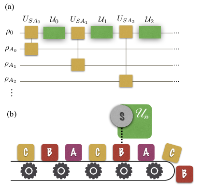
Figure 3: (a) Diagramatic illustration of the collisional model in Eq. (100). (b) Scheme for studying non-equilibrium steady-states (NESSs) obtained when a system is coupled to multiple reservoirs. In this case the ancillas cycle through an alphabet of states, $\rho_{A}$, $\rho_{B}$, $\rho_{C}$, $\rho_{A}$, $\rho_{B}$, $\ldots$ so that the system will never reach equilibrium, even when $\mathcal{U}_{n}=1$ (no unitary strokes).

The states of the ancillas in the collisional model (100) do not have to be identical. This can be used to implement non-trivial limit cycles. The basic idea is illustrated in Fig. 3(b). It consists in setting the ancillas to cycle through an alphabet of $m$ states, such as $\rho_{A}$, $\rho_{B}$, $\rho_{C}$, $\rho_{A}$, $\rho_{B}$, $\rho_{C}$, $\ldots$ in the example of the figure. If the composite map

$$\Phi(\rho_{S})=\mathcal{U}_{m}\circ\mathcal{E}_{m}\circ\ldots\circ\mathcal{U}_{1}\circ\mathcal{E}_{1}(\rho_{S}),$$ (101)

is applied for a sufficiently long time, any transients related to the system’s initial conditions will vanish and the system will reach a limit cycle, characterized by $\rho_{S}^{*}=\Phi(\rho_{S}^{*})$. Because the ancillas are always changing, however, this limit cycle will not be a fixed point of the individual maps (100), only of the composite map (101). As a consequence, the system will never reach a steady-state but will, instead, keep bouncing back and forth within the limit cycle. This can be used to generate a diverse set of rich dynamics describing engine-like behaviour.

For concreteness, we assume that within the system-ancilla strokes the system Hamiltonian remains fixed at $H_{S}^{n}$. During the subsequent unitary stroke, on the other hand, it changes from $H_{S}^{n}$ to $H_{S}^{n+1}$. The precise way through which this change takes place is encoded in the unitary $\mathcal{U}_{n}$. Heat is then defined, as in Sec. III, as the change in energy of the ancillas [cf. Eq. (35)]; i.e., $Q_{A_{n}}:=\operatorname{tr}\big{\{}H_{A_{n}}\big{(}\rho_{A_{n}}^{\prime}-\rho_{A_{n}})\big{\}}$ This is to be compared with the total change in energy of the system,

$$\Delta H_{S}^{n}=\operatorname{tr}\big{(}H_{S}^{n+1}\rho_{S}^{n+1}-H_{S}^{n}\rho_{S}^{n}\big{)}.$$ (102)

The mismatch between $Q_{A_{n}}$ and $\Delta H_{S}^{n}$ is then attributed entirely to work. This work, however, may have a contribution from the on/off work of the system-ancilla interaction and a contribution from the unitary $U_{n}$: rCl W_n^on/off &= tr{ H_S^n[ E_n(ρ_S^n) - ρ_S^n]} +Q_A_n,
W_n^u = tr{ H_S^n+1 ρ_S^n+1 - H_S^n E_n (ρ_S^n)}. The first law therefore decomposes as

$$\Delta U_{S}^{n}=W_{n}^{\text{u}}+W_{n}^{\text{on/off}}+Q_{A_{n}}.$$ (103)

Notice how $\Delta H_{S}^{n}$ in Eq. (102) is a function of state, whereas $Q_{A_{n}}$ and $W_{n}$ are not.

As for the second law, based on the results of Sec. III, we have three tiers of possible expressions for the entropy production: rCl Σ_n &= I_ρ_SA_n’ (S​ : ​ A_n) + S(ρ_A_n’ —— ρ_A_n)
= ΔS_S^n + β_n Q_A_n
= S(ρ_S^n —— ρ_S^n,th) - S(ρ_S^n+1 —— ρ_S^n,th), where $\Delta S_{S}^{n}=S(\rho_{S}^{n+1})-S(\rho_{S}^{n})$ is the change in the entropy of the system in the map (100). The first line is the general definition (26) and holds for any ancillary state. The second line is only true if the ancillas are thermal, not necessarily at the same temperature [Eq. (34)]. Finally, the third line is only true for thermal operations (i.e., if the ancillas are thermal and the unitary satisfies the strict energy conservation condition (48)). If the ancillas are identical, some of the indices $n$ may be dropped and the expressions simplify a bit.

V.2 The emergence of a preferred basis

The classical limit is usually associated with the emergence of a preferred basis in which coherence among the basis elements tend to be suppressed. In the so-called “einselection” paradigm Zurek1981, this basis emerges due to the contact with a heat bath. Thermal operations (Sec. III.4) provide a clear illustration of this principle and also highlight some of the subtle issues that arise in the classical limit.

We consider here the collisional model in Eq. (100) and assume that the ancillary stroke (99) is a thermal operation (Sec. III.4). During the unitary stroke, the Hamiltonian is assumed to change from $H_{S}^{n}=H_{S}(\lambda_{n})$ to $H_{S}^{n+1}=H_{S}(\lambda_{n+1})$, where $\lambda$ represents a generic work parameter. For simplicity, however, we assume that this change is much faster than the system-ancilla stroke, so that we may set $\mathcal{U}_{n}\simeq 1$.

Let $H_{S}^{n}=\sum_{i}E_{i}^{n}|i_{n}\rangle\langle i_{n}|$ denote the spectral decomposition of $H_{S}^{n}$ in terms of the eigenvalues $E^{n}_{i}$ and corresponding eigenstates $|i_{n}\rangle$ at each given time $n$. We assume that the eigenvalues $E_{i}^{n}$ are non-degenerate. As shown in Cwikli2015, if the map (99) is a thermal operation, the populations $\langle i_{n}|\rho_{S}^{n}|i_{n}\rangle$ at the instantaneous eigenstates will evolve according to the classical Markov chain

$$\langle i_{n}|\rho_{S}^{n+1}|i_{n}\rangle=\sum\limits_{j}M_{n}(i|j)\langle j_{n}|\rho_{S}^{n}|j_{n}\rangle,$$ (104)

where $M_{n}(i|j)=\sum_{\mu,\nu}q_{\nu}^{n}|\langle i_{n}\mu_{n}|U_{SA_{n}}|j_{n}\nu_{n}\rangle|^{2}$, with $q_{\nu}^{n}$ and $|\nu_{n}\rangle$, $|\mu_{n}\rangle$ being the initial populations and eigenstates of ancilla $A_{n}$; i.e., $\rho_{A_{n}}=e^{-\beta H_{E}^{n}}/Z_{E}^{n}=\sum_{\nu}q_{\nu}^{n}|\nu_{n}\rangle\langle\nu_{n}|$. We call attention to the fact that, in order to make sure each step is a thermal operation, the states of the ancillas and the unitaries $U_{SA_{n}}$ have to change to adjust to the strict energy conservation condition (46); this makes the above construction difficult to realize exactly, although it is realizable approximately, as we discuss below.

Notice how the left hand side of (104) contains $\langle i_{n}|\rho_{S}^{n+1}|i_{n}\rangle$, which differs in general from $\langle i_{n+1}|\rho_{S}^{n+1}|i_{n+1}\rangle$. This highlights a unique property of quantum dynamics; namely that the action of the work agent may change not only the populations $E_{i}^{n}$ of the system, but also rotate the eigenbasis $|i_{n}\rangle$. The notion of “population and coherences” in Eqs. (104) and (107) should thus be interpreted with care, as they change with each step. As a consequence, even quasi-static dynamics, which are usually somewhat dull for classical systems, may present interesting and highly non-trivial effects, which are of genuine quantum nature. This was recently explored in Ref. Miller2019; Scandi2019 and will be reviewed in Sec. LABEL:sec:inf_quenches.

For the remainder of this Section, we focus on the case where $[H_{S}^{n},H_{S}^{m}]=0$ for all $n,m$. This means that during the work strokes, the energy levels of the system may change, but the orientation of the eigenbasis $|i\rangle$ remains fixed. One may then define the populations $p_{i}^{n}=\langle i|\rho_{S}^{n}|i\rangle$, so that Eq. (104) is converted into the classical Markov chain

$$p_{i}^{n+1}=\sum\limits_{j}M_{n}(i|j)p_{j}^{n}.$$ (105)

The $M_{n}(i|j)$ are simply transition probabilities (their time-dependence comes from the fact that the Hamiltonian may be changing in time). Moreover, as the ancillas are thermal, they satisfy the detailed balance condition

$$M_{n}(i|j)=M_{n}(j|i)e^{-\beta(E_{i}^{n}-E_{j}^{n})}.$$ (106)

Thus, by all standards, the populations evolve according to an entirely classical evolution. Most importantly, the evolution of populations and coherences are completely decoupled. Indeed, the latter are found to evolve according to

$$\langle i|\rho_{S}^{n+1}|j\rangle=\mathcal{R}_{ij}^{n}~{}\langle i|\rho_{S}^{n}|j\rangle,$$ (107)

where $\mathcal{R}_{ij}^{n}=\sum_{\mu,\nu}q_{\nu}^{n}\langle i\nu_{n}|U_{SA_{n}}|i\mu_{n}\rangle\langle j\nu_{n}|U_{SA_{n}}^{\dagger}|j\mu_{n}\rangle$. One may verify that $|\mathcal{R}_{ij}^{n}|<1$ Cwikli2015, so the off-diagonals are suppressed further and further with each collision, until eventually vanishing.

This example clearly shows the emergence of a preferred basis. Due to the strict energy conservation property of thermal operations, the energy basis of the system is selected as a preferred basis by the environment, a process called “environment-induced” selection, or einselection. Crucially, this effect is clearly manifested in the entropy production. The entropy produced at each stroke will be given by Eq. (V.1), with $\rho_{S}^{n,th}=e^{-\beta H_{S}^{n}}/Z_{S}^{n}$. We may now split the relative entropy as

$$S(\rho_{S}^{n}||\rho_{S}^{\text{n,th}})=S(\bm{p}^{n}||\bm{p}^{\text{n,th}})+C(\rho_{S}^{n}),$$ (108)

where $S(\bm{p}^{n}||\bm{p}^{\text{n,th}})$ is the classical relative entropy between the probability distributions $p_{i}^{n}$ and $p_{i}^{n,th}=e^{-\beta E_{i}^{n}}/Z_{S}^{n}$; the classical relative entropy is defined as

$$S(\bm{p}||\bm{q})=\sum\limits_{i}p_{i}\ln p_{i}/q_{i}.$$ (109)

The second term in Eq. (108), on the other hand, is the relative entropy of coherence in the energy eigenbasis $|i\rangle$, $C(\rho_{S}^{n})=S(\bm{p}^{n})-S(\rho_{S}^{n})$. Plugging this in Eq. (V.1) allows us to split the entropy production of each step in two parts Santos2019; Mohammady2020

$$\Sigma_{n}=\Sigma_{n}^{\text{cl}}+\Sigma_{n}^{\text{qu}},$$ (110)

where rCl Σ_n^cl &= S(p^n —— p^n,th) - S(p^n+1 —— p^n,th),
Σ_n^qu = C(ρ