Verifying Stochastic Hybrid Systems with Temporal Logic Specifications via Model Reduction

Abstract.

We present a scalable methodology to verify stochastic hybrid systems. Using the Mori-Zwanzig reduction method, we construct a finite state Markov chain reduction of a given stochastic hybrid system and prove that this reduced Markov chain is approximately equivalent to the original system in a distributional sense. Approximate equivalence of the stochastic hybrid system and its Markov chain reduction means that analyzing the Markov chain with respect to a suitably strengthened property, allows us to conclude whether the original stochastic hybrid system meets its temporal logic specifications. We present the first statistical model checking algorithms to verify stochastic hybrid systems against correctness properties, expressed in the linear inequality linear temporal logic (iLTL) or the metric interval temporal logic (MITL).

1. Introduction

Stochastic hybrid systems, modeling discrete, continuous, and stochastic behavior, arise in many real-world applications ranging from automobiles (jin2014benchmarks, ), smart grids (daniele2017smart, ), and biology (rajkumar2010cyber, ; liu_probabilistic_2011, ; liu_approximate_2012, ; zuliani_statistical_2014, ; gyori2015approximate, ). In these contexts, it is often useful to determine if the models meet their time-dependent design goals. However, the verification problem is computationally very challenging — even for systems with very simple dynamics that exhibit no stochasticity, and for the most basic class of safety properties, namely invariants, the problem of determining if a system meets its safety goals is undecidable (decidable-hybrid98, ). The difficulty of the verification problem largely arises from the fact that the state space of such systems has uncountably many states.

The computational challenge posed by the verification problem is often addressed by constructing a simpler finite state model of the system, and then analyzing the finite state model. The finite state model is typically an abstraction or a conservative over-approximation of the original system, i.e., every behavior of the system is exhibited by the finite state model, but the finite state model may have additional behaviors that are not system behaviors. This approach has been used to verify (efhkost03-2, ; adi03, ; rpv17, ) and design controllers (tabuada_linear_2006, ; kloetzer_fully_2008, ; wongpiromsarn_receding_2010, ; liu2013synthesis, ) for non-stochastic systems, as well as to verify (cv09-2, ; liu_probabilistic_2011, ; liu_approximate_2012, ; tkachev2013formula, ; gyori2015approximate, ) and design controllers (tkachev2013quantitative, ) for stochastic hybrid systems. For such abstractions, if the finite state model is safe then so is the original system. However, if the finite state model is unsafe, then not much can be concluded about the safety of the original system because the finite state model is an over-approximation.

In this paper, we present a scalable approach to the verification of a class of specifications defined by iLTL or MITL (04-iLTL, ; 96-MITL, ) for stochastic hybrid systems, based on constructing a finite state approximation that is “equivalent” to the original system. These specifications reason over the evolution of the probability distributions of the systems, and can express a wide class of safety properties.

To verify these specifications, we construct an approximate bi-simulation between stochastic hybrid systems and finite state Markov chains using the Mori-Zwanzig model reduction method (chorin_optimal_2000, ; beck_model_2009, ). The advantage of bi-simulation is that analyzing the finite state model not only allows us to conclude the safety of the hybrid stochastic system, but also its non-safety. In order to explain the relationship between the Markov chain we construct and the stochastic hybrid system, it is useful to recall that there are two broad approaches to defining the semantics of a stochastic process. One approach is to view a stochastic system as defining a measure space on the collection of executions; by execution here we mean a sequence of states that the system may possibly go through. The other approach is to view the stochastic system as defining a transformation on distributions; in such a view, the behavior of the stochastic model is captured by a sequence of distributions, starting from some initial distribution. For the first semantics (of measures on executions), it has been shown that approximate abstractions can be build between finite state Markov chains and certain classes of stochastic hybrid systems (julius_ApproximationsStochasticHybrid_2009, ; abate_ApproximateModelChecking_2010a, ; abate_ApproximateAbstractionsStochastic_2011, ). However, it has been observed that constructing an approximate “equivalence” between Markov chains and infinite-state systems is very challenging in general (gyori2015approximate, ).

In this paper, we in contrast show that the Mori-Zwanzig reduction method constructs a finite state Markov chain that is approximately equivalent to a stochastic hybrid system with respect to the second semantics. That is, we show that the distribution on states of the Markov chain at any time, is close to the distribution at the same time defined by the stochastic hybrid system (Theorem 3.3), even though there might be no (approximate) probabilistic path-to-path correspondence between the path space of the stochastic hybrid system and that of the Markov chain, as it is required under the first semantics.

Similar to (abate_ApproximateModelChecking_2010a, ; abate_ApproximateAbstractionsStochastic_2011, ), the Mori-Zwanzig reduction is performed via partitioning the state space, although the metric for “equivalence” is different. The approximate equivalence by Mori-Zwanzig reduction can be seen to be similar in spirit to the results first established for non-stochastic, stable, hybrid systems (tabuada_linear_2006, ; Pola20082508, ; girard2010approximately, ), and later extended to stochastic dynamical systems (zamani2012symbolic, ; zamani2014symbolic, ). When compared to (zamani2012symbolic, ; zamani2014symbolic, ), we consider a more general class of stochastic hybrid systems that have multiple modes and jumps with guards and resets. Second, our reduced system is a Markov chain, whereas in (zamani2012symbolic, ; zamani2014symbolic, ) the stochastic system is approximated by a finite state, non-stochastic model. In addition, our notion of distance between the stochastic hybrid system and the reduced system is slightly different.

Having proved that our reduced Markov model is approximately equivalent to the original stochastic hybrid system, we can exploit this to verify stochastic hybrid systems. Approximate equivalence ensures that analyzing the reduced model with respect to a suitably strengthened property, allows us to determine whether the initial stochastic hybrid system meets or violates its requirements. Therefore, a scalable verification approach can be obtained by developing algorithms to verify finite state Markov chains. Since the reduced system, even though finite state, is likely to have a large number of states, we use a statistical approach to verification (younes_statistical_2006, ) as opposed to a symbolic one.

In statistical model checking, the model being verified is simulated multiple times, and the drawn simulations are analyzed to see if they constitute a statistical evidence for the correctness of the model. Statistical model checking algorithms have been developed for logics that reason about measures of executions (younes_statistical_2006, ; sen_statistical_2005, ; yesno-to-yesnounknown-2006-Younes, ; zuliani_statistical_2014, ). However, since our reduced Markov chain is only close to the stochastic hybrid system in a distributional sense, we cannot leverage these algorithms. Instead, we develop new statistical model checking algorithms for temporal logics (over discrete and continuous time) that reason about sequences of distributions.

The scalability of our approach depends critically on the way the partition-based Mori-Zwanzig model reduction is performed, as it involves numerical integrations on the partitions. For stochastic hybrid systems with nonlinear but polynomial dynamics for the continuous part, the curse of dimensionality for direct numerical integration can be avoided as explicit symbolic solutions for the numerical solution exists. This is demonstrated in Section 6 by a case study. Also, Monte-Carlo integrations can be adopted for more general dynamics with considerations on extra statistical errors. Finally, we note that using this approach, we were the first to successfully verify (rwwdv17, ) a highly non-linear model including lookup tables of a powertrain control system that was proposed as a challenging problem for verification tools by Toyota engineers (jin2014benchmarks, ).

This paper is based on three of our previous papers (wang2015statistical, ; Wang2015267, ; wang2016verifying, ), where discrete-time stochastic hybrid systems are studied in (wang2015statistical, ); continuous-time stochastic (non-hybrid) systems are studied in (Wang2015267, ); and continuous-time stochastic hybrid systems are studied in (wang2016verifying, ) without numerical evaluations. This work presents a unification for the statistical verification of continuous-time and discrete-time stochastic hybrid systems, and provides a case study to numerically demonstrate the scalability of our statistical verification algorithms.

The rest of the article is organized as follows. In Section 2, we introduce the general setup of the problem, including the definition of continuous-time stochastic hybrid systems and the syntax and semantics of metric interval temporal logic. In Section 3, we use the Mori-Zwanzig method to reduce the hybrid system to a Markov chain and prove that the temporal logic formulas on the hybrid system can be verified by checking slightly stronger formulas on the Markov chain. In Section 4, we develop a statistical model checking algorithm for actually carrying out the verification. In Section 5, we consider discrete-time stochastic hybrid systems and derive similar model reduction and model checking results in this setting. The scalability of the proposed algorithms is demonstrated by a case study in Section 6. Finally, we conclude in Section 7.

2. Problem Formulation

We denote the set of natural, rational, non-negative rational, real, positive real, and non-negative real numbers by $\mathbb{N}$, $\mathbb{Q}$, $\mathbb{Q}_{\scalebox{0.5}{${\geq}0$}}$, $\mathbb{R}$, $\mathbb{R}_{>0}$ and $\mathbb{R}_{\scalebox{0.5}{${\geq}0$}}$ respectively. We denote the essential supremum by ${\rm ess\ sup}$. For $n\in\mathbb{N}$, let $[n]=\{1,2,\ldots,n\}$. For any set $\mathbb{S}$, let $\mathbb{S}^{\boldsymbol{\omega}}$ be the set of infinite sequences in $\mathbb{S}$. For $s\in\mathbb{S}^{\boldsymbol{\omega}}$, let $s_{i}$ be the $i^{\rm th}$ element in the sequence. For a finite set $A$, we denote the cardinality by $|A|$ and its power set by $2^{A}$. The empty set is denoted by $\emptyset$. For $X\subseteq\mathbb{R}^{d}$, we denote the boundary of $X$ by $\partial X$. The symbols $\mathbb{P}$ and $\mathbb{E}$ are used for the probability and the expected value, respectively.

2.1. Stochastic Hybrid System

In this work, we follow the formal definitions of continuous-time stochastic hybrid systems in (Teel20142435, ; teel2015stochastic, ; Teel2017, ; Subbaraman2017, ) as shown in Fig. 1. However, we focus on a Fokker-Planck formulation and interpretation of the model.

2.1.1. Continuous-time Stochastic Hybrid System

We denote the continuous and discrete states by $x\in\mathbb{R}^{d}$ and $q\in\mathcal{Q}$ respectively, where $\mathcal{Q}=\{q_{1},\ldots,q_{m}\}$ is a finite set. We call the combination $(q,x)$ the state of the system, and the product set $\mathbb{X}\subseteq\mathcal{Q}\times\mathbb{R}^{d}$ the state space. For each $q\in\mathcal{Q}$, the state of the system flows in $\mathbf{A}_{q}\subseteq\mathbb{R}^{d}$ and jumps forcedly on hitting the boundary $\mathbf{A}_{q}$. We assume that each $\mathbf{A}_{q}$ is open and bounded, and the boundaries $\partial\mathbf{A}_{q}$ are second-order continuously differentiable. On the flow set, the state $x$ of the system evolves by a stochastic differential equation

(1) $$\mathrm{d}x=f(q,\mathbf{x})\mathrm{d}t+g(q,\mathbf{x})\mathrm{d}B_{t},$$

where $q$ and $\mathbf{x}$ are random processes describing the stochastic evolution of the discrete and continuous states, and $B_{t}$ is the standard $n$-dimensional Brownian motion. The vector-valued function $f$ specifies the drift of the state, and the matrix-valued function $g$ describes the intensity of the diffusion (karatzas2012brownian, ; revuz2013continuous, ). In (1), we assume that $f(q,\cdot)$ and $g(q,\cdot)$ are locally Lipschitz continuous. Meanwhile, the system jumps spontaneously by a non-negative integrable rate function $r(q,x)$ inside $\mathbf{A}_{q}$. The probability distribution of the target of both spontaneous and forced jumps (as they happened on different domains) is given by a non-negative integrable target distribution $h(q^{\prime},x^{\prime},q,x)$, satisfying

(2) $$\sum_{q\in\mathcal{Q}}\int_{\mathbf{A}_{q}}h(q^{\prime},x^{\prime},q,x)\mathrm{d}x^{\prime}=1.$$

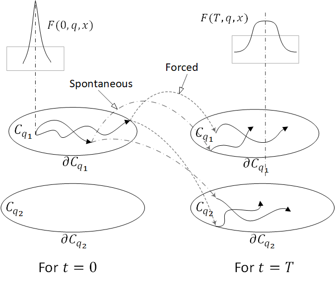
Figure 1. A continuous-time stochastic hybrid system with two discrete states at time $0$ and $T$.

2.1.2. Fokker-Planck Equation

The probability distribution $F(t,q,x)$ of the state of the system in the flow set is determined by the Fokker-Planck equation, which can be derived in the same way as that for jump-diffusion processes (hanson_AppliedStochasticProcesses_2007, ),

(3) $$\begin{split}&\frac{\partial F(t,q,x)}{\partial t}=L(F(t,q,x))=\underbrace{-\sum_{a=1}^{d}\frac{\partial}{\partial x_{a}}(f_{a}(q,x)F(t,q,x))}_{\rm drift}\underbrace{+\sum_{a=1}^{d}\sum_{b=1}^{d}\frac{\partial^{2}}{\partial x_{a}\partial x_{b}}\sum_{c=1}^{d}\frac{g_{ac}(q,x)g_{cb}(q,x)F(t,q,x)}{2}}_{\rm diffusion}\\ &\quad\underbrace{-r(q,x)F(t,q,x)}_{\textrm{jump out}}\underbrace{+\sum_{q\in\mathcal{Q}}\int_{x\in\mathbb{A_{q}}}h(q,x,q^{\prime},x^{\prime})r(q^{\prime},x^{\prime})F(t,q^{\prime},x^{\prime})\mathrm{d}x^{\prime}}_{\textrm{spontaneous jump in}},\underbrace{+\sum_{q\in\mathcal{Q}}\int_{x\in\partial\mathbb{A_{q}}}h(q,x,q^{\prime},x^{\prime})(\mathbf{n}\cdot\mathbf{F})\mathrm{d}x^{\prime}}_{\textrm{forced jump in}},\end{split}$$

where $f_{a}$ is the $a$th element of $f$ from (1), $\mathbf{n}$ is the unit vector pointing out of the flow set and the inner product $\mathbf{n}\cdot\mathbf{F}$ is the corresponding outgoing flow. Here, $\mathbf{F}$ is a matrix (more precisely a second-order tensor) whose components are given by

(4) $$\mathbf{F}_{ab}=\frac{\partial}{\partial x_{b}}\sum_{c=1}^{d}\frac{g_{ac}(q,x)g_{cb}(q,x)F(t,q,x)}{2},$$

where $a,b\in[d]$. In (3), $L$ is the Fokker-Planck operator for the system, and we write symbolically that $F(t,q,x)=e^{tL}F(0,q,x)$. On the boundary, we have

(5) $$F(t,q^{\prime},x^{\prime})=0$$

as it is absorbing (paths jump away immediately after hitting the boundary). In the rest of the paper, we assume that the stochastic hybrid system given in this section is well defined in the sense that it gives a Fokker-Planck equation with a unique solution (karatzas2012brownian, ; revuz2013continuous, ).

2.1.3. Invariant Distribution

An invariant distribution of the continuous-time stochastic hybrid system $F_{\rm inv}(q,x)$ is defined by

(6) $$L(F_{\rm inv}(q,x))=0.$$

In this work, when handling temporal logic specifications of an infinite time horizon, we assume that $F(t,q,x)$ converges to the invariant distribution function $F_{\rm inv}(q,x)$ to ensure that the truth value of the specifications will not change after a finite time.

2.1.4. System Observables

The state of the system is only partially observable. Here, we are interested in observables of the system given by

(7) $$y(t)=\mathbb{E}[y(q(t),x(t))]=\sum_{q\in\mathcal{Q}}\int_{\mathbf{A}_{q}}\gamma(q,x)F(t,q,x)\mathrm{d}x,$$

where $\gamma(q,x)$ is a weight function on $\mathbb{X}$, which is integrable in $x$ for each $q\in\mathcal{Q}$.

Example 2.1.

Throughout the paper, we use the following example to illustrate the theorems. Consider a continuous-time stochastic hybrid system with two discrete states on $\mathbb{X}=\{1\}\times[0,1]\cup\{2\}\times[2,4]$. It jumps uniformly to $[2,4]$ when hitting $x=0$ or $x=1$, and jumps uniformly to $[0,1]$ when hitting $x=2$ or $x=4$. It can jump spontaneously at any $x\in\mathbb{X}$ with the rate $h(x)=\mathbf{I}_{\mathbb{X}}(x)/3$, where $\mathbf{I}_{\mathbb{X}}(\cdot)$ is the indicator function of the set $\mathbb{X}$. In each location, the state of the system is governed by the stochastic differential equation

$$\mathrm{d}\mathbf{x}=\mathrm{d}t+\mathrm{d}B_{t},$$

The probability distribution $F(t,q,x)$ of the state evolves by the Fokker-Planck equation

$$\begin{split}&\frac{\partial F(t,q,x)}{\partial t}=-\frac{\partial F(t,q,x)}{\partial x}+\frac{1}{2}\frac{\partial^{2}F(t,q,x)}{\partial x^{2}}+\frac{\partial F(t,q,0)}{\partial x}-\frac{\partial F(t,q,1)}{\partial x}+\frac{1}{2}\frac{\partial F(t,q,2)}{\partial x}-\frac{1}{2}\frac{\partial F(t,q,4)}{\partial x}\end{split}$$

with the boundary conditions

$$F(t,q,0)=F(t,q,1)=F(t,q,2)=F(t,q,4)=0.$$

Initially, the state of the system is uniformly distributed on $[0,1/2]$.

2.2. Metric Interval Temporal Logic

We are interested in verifying temporal properties of the continuous-time stochastic hybrid systems. These properties are specified as follows. The atomic propositions $\mathtt{AP}$ are inequalities of the form $y\sim c$ ($c\in\mathbb{Q}$, $\sim\in\{<,\leq,\geq,>\}$), where $y$ is an observable of the system given by (7); and these atomic propositions are concatenated by the syntax of Metric Interval Temporal Logic (MITL) (96-MITL, ). This type of logic is also referred to as Signal Temporal Logic (STL) (04-STL, ; 15-monSTL, ; 13-monSTL, ) in the literature. The syntax of MITL is given in Definition 2.2.

Definition 2.2 (MITL Syntax).

An MITL formula is defined using the following BNF form:

$$\varphi\Coloneqq\bot\mid\top\mid y\sim c\mid\varphi\land\varphi\mid\varphi\lor\varphi\mid\varphi\mathcal{U}_{I}\varphi\mid\varphi\mathcal{R}_{I}\varphi,$$

where $c\in\mathbb{Q}$, $\sim\in\{<,\leq,\geq,>\}$ and $I$ is a non-singleton interval on $\mathbb{R}_{\scalebox{0.5}{${\geq}0$}}$.

We note that the syntax does not contain negation ($\neg$), since $\{<,\leq,\geq,>\}$ is closed under negation. For a standard MITL formula, negation on non-atomic formulas can always be pushed inside as part of the atomic propositions. For example, $\neg\lparen y>0\rparen$ is defined as $y\leq 0$, $\neg\lparen\varphi_{1}\vee\varphi_{2}\rparen$ is defined as $\lparen\neg\varphi_{1}\rparen\land\lparen\neg\varphi_{2}\rparen$, and $\neg\lparen\varphi\mathcal{U}_{I}\psi\rparen$ is defined as $\lparen\neg\varphi\rparen\mathcal{R}_{I}\lparen\neg\psi\rparen$.

The continuous-time stochastic hybrid system induces a signal $f(t):\mathbb{R}_{\scalebox{0.5}{${\geq}0$}}\rightarrow 2^{\mathtt{AP}}$ by $(y\sim c)\in f(t)$ iff $y\sim c$ holds at time $t$. The semantics of MITL are defined with respect to the signal $f(t)$ as follows.

Definition 2.3 (MITL Semantics).

Let $\varphi$ be an MITL formula and $f$ be a signal $f:\mathbb{R}_{\scalebox{0.5}{${\geq}0$}}\rightarrow 2^{\mathtt{AP}}$. The satisfaction relation $\models$ between $f$ and $\varphi$ is defined according to the following inductive rules:

$$\begin{array}[]{@{}l@{\ }c@{\ }l@{}}f\models\bot&{\rm iff}&\mbox{false}\\ f\models\top&{\rm iff}&\mbox{true}\\ f\models y\sim c&{\rm iff}&\lparen y\sim c\rparen\in f(0)\\ f\models\varphi\land\psi&{\rm iff}&\lparen f\models\varphi\rparen\land\lparen f\models\psi\rparen\\ f\models\varphi\lor\psi&{\rm iff}&\lparen f\models\varphi\rparen\lor\lparen f\models\psi\rparen\\ f\models\varphi\mathcal{U}_{I}\psi&{\rm iff}&\exists t\in I,\lparen f^{t}\models\psi\rparen\land\forall t^{\prime}\in(0,t),f^{t^{\prime}}\models\varphi\\ f\models\varphi\mathcal{R}_{I}\psi&{\rm iff}&\forall t\in I,\lparen f^{t}\models\psi\rparen\textrm{ or }\exists t\in\mathbb{R}_{>0},(f^{t}\models\varphi\land\forall t^{\prime}\in[0,t]\cap I,f^{t^{\prime}}\models\psi)\textrm{ or }\\ &&\exists t\in I^{\prime},t^{\prime}\in I\cap(t,\infty),\forall t^{\prime\prime}\in I,(t^{\prime\prime}\leq t\to f^{t^{\prime\prime}}\models\psi)\land(t<t^{\prime\prime}\leq t^{\prime}\to f^{t^{\prime\prime}}\models\varphi)\end{array}$$

where $f^{r}(\cdot)=f(r+\cdot)$ and $I^{\prime}=I\cup\{\underline{I}\}$ in the semantics of $\varphi\mathcal{R}_{I}\psi$ with $\underline{I}$ being the lower bound of $I$. We define $\llbracket\varphi\rrbracket$ to be the set of signals that satisfy $\varphi$.

Our semantics of $\mathcal{R}$ in MITL is more complicated than the semantics of $\mathcal{R}$ in LTL, its discrete-time counterpart. Our semantics of $\mathcal{R}$ is also different from the common semantics of MITL (96-MITL, ). This is because it has recently been shown that the common semantics of MITL cannot ensure that the formulas $\neg(\varphi\mathcal{U}_{I}\psi)$ and $(\neg\varphi)\mathcal{R}_{I}(\neg\psi)$ are equivalent for the continuous-time domain (see (roohi2018revisiting, ) for details). Following the semantics of MITL, the satisfiability/model checking problems for MITL with abstract atomic propositions are known to be EXPSPACE -complete (96-MITL, ; roohi2018revisiting, ). The corresponding decision procedure has a close connection with timed automata.

Definition 2.4 (Timed Automata (94-TA, )).

timed automaton $A$ is a tuple $(\mathtt{Q},\mathtt{X},\Sigma,\mathtt{L},\mathtt{I},\mathtt{E},\mathtt{Q}^{\mathsf{init}},\mathtt{Q}^{\mathtt{final}})$ where

• $\mathtt{Q}$ is a finite non-empty set of locations.

• $\mathtt{X}$ is a finite set of clocks.

• $\Sigma$ is a finite alphabet.

• $\mathtt{L}:\mathtt{Q}\rightarrow\Sigma$ maps each location to the label of that location.

• $\mathtt{I}:\mathtt{Q}\rightarrow(\mathtt{X}\rightarrow{\mathbb{I}}_{\geq 0})$ maps each location to its invariant which is the set of possible values of variables in that location, where ${\mathbb{I}}_{\geq 0}$ is the set of intervals on $\mathbb{R}_{\scalebox{0.5}{${\geq}0$}}$.

• $\mathtt{E}\subseteq\mathtt{Q}\times\mathtt{Q}\times 2^{\mathtt{X}}$ is a finite set of edges of the form $e=(s,d,j)$, where $s=\mathtt{S}e$ is source of the edge; $d=\mathtt{D}e$ is destination of the edge; and $j=\mathtt{J}e$ is the set of clocks that are reset by the edge.

• $\mathtt{Q}^{\mathsf{init}}\subseteq\mathtt{Q}$ is the set of initial locations.

• $\mathtt{Q}^{\mathtt{final}}\subseteq\mathtt{Q}$ is the set of final locations.

A run of the timed automaton $A$ is a sequence of tuples $\lparen\rho,\tau,\eta\rparen\in\mathtt{Q}^{\omega}\times{\mathbb{I}}^{\omega}_{\geq 0}\times\mathtt{E}^{\omega}$ in which the following conditions holds: (i) $\rho_{0}\in\mathtt{Q}^{\mathsf{init}}$, i.e., $\rho$ starts from an initial location $\mathtt{Q}^{\mathsf{init}}$; (ii) $(\mathtt{S}\eta_{n}=\rho_{n})\land(\mathtt{D}\eta_{n}=\rho_{n+1})$, i.e., the source and destination of edge $\eta_{n}$ is $\rho_{n}$ and $\rho_{n+1}$, respectively; (iii) $\tau_{0},\tau_{1},\ldots$is an ordered and disjoint partition of the time horizon $\mathbb{R}_{\scalebox{0.5}{${\geq}0$}}$; and (iv) $\forall t\in\tau_{n},x\in\mathtt{X}$, we have $\varrho_{n}(x)+t-\underline{\tau}_{n}\in\mathtt{I}(\rho_{n},x)$, where $\varrho_{0}(x)=0$ and $\varrho_{n+1}(x)$ is inductively defined by $$\displaystyle\varrho_{n+1}(x)=\begin{cases}0,&\text{ if }x\in\mathtt{J}\eta_{n}\\ \varrho_{n}(x)+\overline{\tau}_{n}-\underline{\tau}_{n},&\text{ otherwise}\end{cases}$$ i.e., clocks must satisfy the invariant of the current location. Here, $\underline{\tau}$ and $\overline{\tau}$ are the lower and upper bound of the interval.

A run satisfying the condition $\mathtt{inf}\lparen\rho\rparen\cap\mathtt{Q}^{\mathtt{final}}\neq\emptyset$, i.e., some location from $\mathtt{Q}^{\mathtt{final}}$ has been visited infinitely many times by $\rho$, is called an accepting run of $A$. Note that every run of $A$ induces a function $f$ of type $\mathbb{R}_{\scalebox{0.5}{${\geq}0$}}\rightarrow\Sigma$ that maps $t$ to $\mathtt{L}(\rho_{n})$, where $n$ is uniquely determined by the condition $t\in\tau_{n}$. We define the language of $A$, denoted by $\mathtt{Lang}\lparen A\rparen$, to be the set of all functions that are induced by accepting runs of $A$. The language of timed automata is closely related to MITL as follows.

Lemma 2.5 (MITL to Timed Automata (96-MITL, )).

For any MITL formula $\varphi$, a timed automaton $A_{\varphi}$ can be constructed such that $\mathtt{Lang}\lparen A_{\varphi}\rparen=\llbracket\varphi\rrbracket$, i.e., the set of functions that satisfy $\varphi$ is exactly those that are induced by accepting runs of $A_{\varphi}$.

Example 2.6.

Following Example 2.1, we want to check the following MITL formula

$$\varphi_{1}=\top\ \mathcal{U}\left(y_{2}(t)>\frac{1}{4}\right),\quad\varphi_{2}=\left(y_{1}(t)>\frac{1}{2}\right)\mathcal{U}\left(y_{2}(t)>\frac{1}{4}\right),$$

where

$$y_{1}(t)=\sum_{q\in\mathcal{Q}}\int_{\mathbf{A}_{q}}I_{[0,1]}F(t,q,x)\mathrm{d}x,\quad y_{2}(t)=\sum_{q\in\mathcal{Q}}\int_{\mathbf{A}_{q}}I_{[2,4]}F(t,q,x)\mathrm{d}x.$$

3. Model Reduction of Continuous-time Hybrid Systems

The model reduction procedure for continuous-time stochastic hybrid system follows the three steps: (i) reduce the dynamics by partitioning the state space; (ii) reduce the temporal logic specifications accordingly; and (iii) estimate the model reduction error.

3.1. Reducing the Dynamics

To implement the Mori-Zwanzig model reduction method (chorin_optimal_2000, ) for continuous-time stochastic hybrid systems, we partition the continuous state space into finitely many partitions $\mathbb{S}=\{s_{1},\ldots,s_{n}\}$, and treat each of them as a discrete state. The idea of partitioning is similar to (abate_ApproximateModelChecking_2010a, ; abate_ApproximateAbstractionsStochastic_2011, ) for the discrete-time stochastic hybrid systems. The partition is called an equipartition if they are hypercubes with the same size $\eta$. We assume that for each $s_{i}$, there exists $q\in\mathcal{Q}$ such that $s_{i}\subseteq\{q\}\times\mathbf{A}_{q}$, and denote its measure by $\mu(s_{i})$. Let $m(\mathbb{X})$ and $m(\mathbb{S})$ be sets of probability distribution functions on $\mathbb{X}$ and $\mathbb{S}$, respectively. Then we can define a projection $P:m(\mathbb{X})\rightarrow m(\mathbb{S})$ and an injection $R:m(\mathbb{S})\rightarrow m(\mathbb{X})$ between $m(\mathbb{X})$ and $m(\mathbb{S})$ by

(8) $$p_{j}=(PF(q,x))_{j}=\int_{s_{j}}F(q,x)\mathrm{d}x,$$

where $p_{j}$ is the $j$th element of $p$, and

(9) $$Rp=\sum_{j=1}^{n}p_{j}\mathbf{U}_{s_{j}},$$

where $\mathbf{U}_{s_{j}}$ is the uniform distribution on $s_{j}$:

(10) $$\mathbf{U}_{s_{j}}(x)=\begin{cases}\frac{1}{\mu(s_{j})},&\text{ if }x\in s_{j}\\ 0,&\text{ otherwise.}\end{cases}$$

Here the projection $P$ and the injection $R$ are defined for probability distributions. But they extend naturally to $L_{1}$ functions on $\mathbb{X}$ and $\mathbb{S}$ respectively. The projection $P$ is the left inverse of the injection $R$ but not vice versa, namely $PR=I$ but $RP\neq I$.

This projection $P$ and injection $R$ can reduce the Fokker-Planck operator to a transition rate matrix on $\mathbb{S}$, and hence reduce the continuous-time stochastic hybrid system into a continuous-time Markov chain. Following (chorin_optimal_2000, ), the Fokker-Planck operator given in (3) reduces to the transition rate matrix $A$ by

(11) $$A=PLR$$

In practice, we are usually interested in a continuous state space $\mathbb{X}$ that is partitioned into hypercubes of edge length $\eta$. In this case, the transition rate matrix $A$ is explicitly expressed as follows.

Theorem 3.1.

Let $\mathbb{S}=\{s_{1},s_{2},\ldots,s_{n}\}$ be a partition of the $d$-dimensional continuous state space $\mathbb{X}$ into hypercubes of edge length $\eta$, and $P$ and $R$ be the corresponding projection and injection given by (8)-(10), the transition rate from the state $s_{i}$ to the state $s_{j}$ ($i\neq j$) at time $t$ is given by

(12) $$\begin{split}A_{ij}=\mathbf{n}\cdot\big{(}\mathbf{N}+\frac{\mathbf{M}\cdot\mathbf{n}(p_{i}-p_{j})}{\eta}\big{)}+\mathbf{R}\end{split}$$

for $a,b\in[n]$, where $\mathbf{n}$ is (if exists) the unit vector of the boundary $s_{i}\cap s_{j}$ pointing from $s_{i}$ to $s_{j}$, $\mathbf{N}$ is a $d$ dimensional vector with components

(13) $$\mathbf{N}_{a}=\int_{\partial s_{i}\cap\partial s_{j}}f_{a}(q,x)\mathrm{d}x,$$

$\mathbf{M}$ is a $d\times d$ matrix with components

(14) $$\mathbf{M}_{ab}=\int_{\partial s_{i}\cap\partial s_{j}}\sum_{c=1}^{d}\frac{g_{ac}(q,x)g_{cb}(q,x)}{2}\mathrm{d}x,$$

and for an inner cell $s_{i}$,

(15) $$\mathbf{O}=\int_{s_{i}\times s_{j}}\frac{\mathbf{I}_{s_{j}}(q,x)h(q,x,q^{\prime},x^{\prime})r(q^{\prime},x^{\prime})\mathbf{I}_{s_{i}}(q^{\prime},x^{\prime})}{\eta^{d}}\mathrm{d}x^{\prime}\mathrm{d}x$$

for a boundary cell $s_{j}$,

(16) $$\mathbf{O}=\int_{s_{i}\times s_{j}}\frac{\mathbf{I}_{s_{j}}(q,x)h(q,x,q^{\prime},x^{\prime})\mathbf{n^{\prime}}\cdot\mathbf{M}\cdot\mathbf{n^{\prime}}p_{i}}{\eta/2;}\mathrm{d}x^{\prime}\mathrm{d}x$$

with $\mathbf{I}_{s_{i}}$ being the indicator function of $s_{i}$ and $\mathbf{n^{\prime}}$ being the vector pointing out of the boundary of the flow set.

Proof.

For simplicity, we first show the proof for the 1D case. Specifically, for fixed $q$, we integrate both sides of (3) on the cell $I=[p,p+\Delta p]$, and apply the Stokes theorem for the first two terms, we derive

(17) $$\begin{split}&\int_{I}\frac{\partial F(t,q,x)}{\partial t}\mathrm{d}x=-f(q,x)F(t,q,x)\Big{|}^{p+\Delta_{p}}_{p}+\frac{\partial}{\partial x}\frac{g^{2}(q,x)F(t,q,x)}{2}\Big{|}^{p+\Delta_{p}}_{p}-\int_{I}r(q,x)F(t,q,x)\mathrm{d}x\\ &\quad+\sum_{q\in\mathcal{Q}}\int_{x\in\mathbb{A_{q}}}\int_{I}h(q,x,q^{\prime},x^{\prime})r(q^{\prime},x^{\prime})F(t,q^{\prime},x^{\prime})\mathrm{d}x\mathrm{d}x^{\prime}+\sum_{q\in\mathcal{Q}}\int_{x\in\partial\mathbb{A_{q}}}\int_{I}h(q,x,q^{\prime},x^{\prime})(\mathbf{n}\cdot\mathbf{F})\mathrm{d}x\mathrm{d}x^{\prime}.\end{split}$$

The left-hand side of (17) is the rate of probability change in the cell $I$. On the right-hand side of (17), (i) the combination of the first two terms $f(q,x)F(t,q,x)-\frac{\partial}{\partial x}\frac{g^{2}(q,x)F(t,q,x)}{2}$ is the probability flow on the boundary; (ii) the other terms correspond to average probability jumps inside the cell $I$. The same is true for multidimensional cases.

By applying (11), it is easy to check the probability flow between adjacent cells sharing a boundary is (14) and (13). The probability of jumping from one inner cell to another cell has the rate (15). Finally, the probability of jumping from one boundary cell to another cell has the rate (16). Thus, (12) holds. ∎

Roughly speaking, the transition rate between two partitions in the same location is the flux of $f(q,x)$ across the boundary and the transition rate between two different locations is the flux of $r(q,x)$.

3.2. Reducing MITL Formulas

The observables on the continuous-time stochastic hybrid system reduce to the corresponding continuous-time Markov chain using the projection $P$. Let $y$ be an observable on the continuous-time stochastic hybrid system with weight function $\gamma(q,x)$. To facilitate further discussion, we assume that $\gamma(q,x)$ is invariant under the projection $P$, i.e.,

(18) $$\gamma(q,x)=RP\gamma(q,x),$$

which means that the function $\gamma(q,x)$ can be written as the linear combination of the indicator functions of the partitions (sometimes called a simple function.) We define a corresponding observable $y^{\prime}$ on the continuous-time Markov chain that derives from the model reduction procedure by

(19) $$\begin{split}y^{\prime}(0)&=\sum_{q\in\mathcal{Q}}\int_{\mathbf{A}_{q}}\gamma(q,x)PF(0,q,x)\mathrm{d}x=\sum_{i=1}^{n}\left(\int_{s_{i}}\gamma(q,x)\mathrm{d}x\right)\left(\int_{s_{i}}F(0,q,x)\mathrm{d}x\right)=\sum_{i=1}^{n}r_{i}p(i).\end{split}$$

From now on, we will always denote the corresponding observable on the CTMC by $y^{\prime}$ for any observable $y$ on the continuous-time stochastic hybrid system.

3.3. Reduction Error Estimation

For a given observable $y$ with weight function $\gamma(q,x)$, the error of the projection $P$ with respect to the observable $y$ is defined by the maximal possible difference between $y$ and $y^{\prime}$,

(20) $$\begin{split}\Delta_{y}=\Big{|}\sum_{q\in\mathcal{Q}}\int_{\mathbf{A}_{q}}\gamma(q,x)(F(0,q,x)-RPF(0,q,x))\mathrm{d}x\Big{|}.\end{split}$$

Remark 1.

When refining the partition of $\mathbb{X}$, $RP\rightarrow I$ in the weak operator topology (rudin1973functional, ); that is, any distribution function $F(q,x)$ on the state space, $|\sum_{q\in\mathcal{Q}}\int_{\mathbf{A}_{q}}\gamma(q,x)(F(q,x)-RPF(q,x))|\rightarrow 0$ holds for any measurable weight function $\gamma(q,x)$. Accordingly for (20), $\Delta_{y}\rightarrow 0$ for any given $y$.

By the definition of $\Delta_{y}$, we know that, at the initial time, the atomic propositions on the continuous-time stochastic hybrid system and the CTMC have the relations

$$y(0)>c\Longrightarrow y^{\prime}(0)>c-\Delta_{y},\quad y(0)<c\Longrightarrow y^{\prime}(0)<c+\Delta_{y},$$

and similarly,

$$y^{\prime}(0)>c+\Delta_{y}\Longrightarrow y(0)>c,\quad y^{\prime}(0)<c-\Delta_{y}\Longrightarrow y(0)<c.$$

To derive the relations of the observables between the continuous-time stochastic hybrid system and the CTMC at any time, we define the reduction error of the observable $y$ at time $t$ due to the model reduction process by

(21) $$\begin{split}\Theta_{y}(t)=|y(t)-y^{\prime}(t)|=\Big{|}\sum_{q\in\mathcal{Q}}\int_{\mathbf{A}_{q}}\gamma(q,x)(e^{Lt}-Re^{At}P)F(0,q,x)\mathrm{d}x\Big{|},\end{split}$$

where $F(0,q,x)$ is an initial distribution of the continuous-time stochastic hybrid system and $y^{\prime}(t)$ is the corresponding observable of $y(t)$ on the CTMC. This reduction error is illustrated in Fig. 2. Note that the diagram is not commutative; the difference between going along the two paths is related to the reduction error.

Figure 2. Diagram for reduction error.

In general, the reduction error $\Theta(t)$ may not be bounded as $t\rightarrow\infty$. To find a sufficient condition for boundedness, we define the reduction error of the Fokker-Planck operator $L$ by

(22) $$\delta(t,q,x)=(L-RPL)e^{tRPL}F(0,q,x).$$

Accordingly, we define the integration of $\delta(t,q,x)$ with respect to the weight function $\gamma(q,x)$ by

(23) $$\begin{split}\Lambda_{y}=\sup_{t\geq 0}\Big{|}\sum_{q\in\mathcal{Q}}\int_{\mathbf{A}_{q}}\gamma(q,x)(L-RPL)e^{tRPL}F(0,q,x)\mathrm{d}x\Big{|},\end{split}$$

which captures the maximal change of the time derivative of observable $y$. When the reduction error $\delta(t,q,x)$ converges exponentially in time, an upper bound of the reduction error $\Theta(t)$ can be obtained.

Definition 3.2.

For $\alpha>0$, $\beta\geq 1$ and a given observable $y$, the continuous-time stochastic hybrid system is $\alpha$-contractive with respect to $y$, if for any initial distribution function $F(0,q,x)$ on the state space, we have

(24) $$\begin{split}&\Big{|}\sum_{q\in\mathcal{Q}}\int_{\mathbf{A}_{q}}\gamma(q,x)e^{tL}\delta(t,q,x)\mathrm{d}x\Big{|}\leq\beta e^{-\alpha t}\Big{|}\sum_{q\in\mathcal{Q}}\int_{\mathbf{A}_{q}}\gamma(q,x)\delta(t,q,x)\mathrm{d}x\Big{|}.\end{split}$$

where $\delta(t,q,x)$ is given by (22).

This contractivity condition is to ensure that the model reduction error is bounded for all time, which is required for approximately keeping the truth value of temporal logic specifications of an infinite time horizon. Although the condition seems restrictive, it is valid for a relatively wide range of systems including asymptotically stable systems. It is a commonly-used sufficient condition to guarantee the existence and uniqueness of an invariant measure for general dynamical systems, and the contractivity factor $\alpha$ is usually derived case-by-case. Using Definition 3.2, we obtain the following theorem.

Theorem 3.3.

If the continuous-time stochastic hybrid system from Section 2.1.1 is $\alpha$-contractive, then for any $t\geq 0$, the reduction error $\Theta_{y}(t)$ for an observable $y$ satisfies

(25) $$\Theta_{y}(t)\leq\frac{\beta\Lambda_{y}}{\alpha}+\Delta_{y}.$$

Proof.

By Dyson’s formula (chorin_optimal_2000, ), we can decompose the exponential of $L$ by

(26) $$e^{tL}=e^{tRPL}+\int_{[0,t]}e^{(t-\tau)L}(L-RPL)e^{\tau RPL}\mathrm{d}\tau,$$

which can be verified by taking time derivatives on both sides. Substituting (26) into (21) gives

(27) $$\begin{split}\Theta_{y}(t)\leq&\Big{|}\sum_{q\in\mathcal{Q}}\int_{\mathbf{A}_{q}}\gamma(q,x)(e^{tRPL}-Re^{tA}P)F(0,q,x)\mathrm{d}x\Big{|}\\ &+\Big{|}\sum_{q\in\mathcal{Q}}\int_{{}^{d}\times[0,t]}\gamma(q,x)e^{(t-\tau)L}(L-RPL)e^{\tau RPL}F(0,q,x)\mathrm{d}\tau\mathrm{d}x\Big{|}\end{split}$$

Since the projection $P$ and the injection $R$ preserve the $L_{1}$ norm, $RPL$ is also a Fokker-Planck operator. Noting $Re^{tA}PF(0,q,x)=e^{tRPL}PF(0,q,x)$, by (20), we see that the first term on the right-hand side of (27) is less than $\Delta_{y}$.

For the second term on the right-hand side of (27), by (23)-(24), we have

(28) $$\begin{split}&\Theta_{y}(t)\leq\Delta_{y}+\Big{|}\sum_{q\in\mathcal{Q}}\int_{\mathbf{A}_{q}}\int_{[0,t]}\gamma(q,x)e^{(t-\tau)L}\delta(\tau,q,x)\mathrm{d}\tau\mathrm{d}x\Big{|}\\ &\leq\Delta_{y}+\Big{|}\sum_{q\in\mathcal{Q}}\int_{\mathbf{A}_{q}}\int_{[0,t]}\beta e^{-\alpha(t-\tau)}\gamma(q,x)\delta(\tau,q,x)\mathrm{d}\tau\mathrm{d}x\Big{|}\leq\frac{\beta\Lambda_{y}}{\alpha}+\Delta_{y}.\end{split}$$

∎

Theorem 3.3 implies the following relations between the atomic propositions on the continuous-time stochastic hybrid system and the CTMC.

Theorem 3.4.

If the continuous-time stochastic hybrid system given in Section 2.1.1 is $\alpha$-contractive, then we have

(29) $$y(t)>c\Longrightarrow y^{\prime}(t)>c-\Big{(}\frac{\beta\Lambda_{y}}{\alpha}+\Delta_{y}\Big{)},$$

(30) $$y(t)<c\Longrightarrow y^{\prime}(t)<c+\Big{(}\frac{\beta\Lambda_{y}}{\alpha}+\Delta_{y}\Big{)},$$

and similarly,

(31) $$y^{\prime}(t)>c+\Big{(}\frac{\beta\Lambda_{y}}{\alpha}+\Delta_{y}\Big{)}\Longrightarrow y(t)>c,$$

(32) $$y^{\prime}(t)<c-\Big{(}\frac{\beta\Lambda_{y}}{\alpha}+\Delta_{y}\Big{)}\Longrightarrow y(t)<c.$$

In Theorem 3.4, the term $\Delta_{y}$ bounds the initial model reduction error and the term $\frac{\beta\Lambda_{y}}{\alpha}$ bounds the model reduction error accumulated over time. Following Theorem 3.4, to verify an MITL formula $\varphi$ for an $\alpha$-contractive continuous-time stochastic hybrid system introduced in Section 2.1.1, we can strengthen $\varphi$ to $\psi$ by replacing the atomic propositions according to (31)-(32). If $\psi$ holds for the CTMC derived from the continuous-time stochastic hybrid system following the model reduction procedure of Sections 3.1 and 3.2, then $\varphi$ holds for the continuous-time stochastic hybrid system.

Example 3.5.

Following Example 2.1 and 2.6, the invariant distribution of this process is $F_{\rm inv}=\mathbf{U}_{\mathbb{X}}/3$. We partition $\mathbb{X}$ into intervals of length $1/N$. By the above model reduction procedure it reduces to a CTMC with transition rate matrix $M$ given by

$$M_{ij}=\frac{\delta_{ij}}{4}+\frac{1}{4N}$$

where $i\in[3N]$ and $j\in[3N]$. The invariant distribution $F_{\rm inv}$ remains unchanged, and the MITL formula to check is

$$\varphi_{1}^{\prime}=\top\ \mathcal{U}\left(y_{2}^{\prime}(t)>\frac{1}{4}+{\Theta_{y}(t)}\right)$$

$$\varphi_{2}^{\prime}=\left(y_{1}^{\prime}(t)>\frac{1}{2}+{\Theta_{y}(t)}\right)\mathcal{U}\left(y_{2}^{\prime}(t)>\frac{1}{4}+{\Theta_{y}(t)}\right)$$

where ${\Theta_{y}(t)}$ is the model reduction error and

$$y_{1}^{\prime}(t)=\sum_{i=1}^{N}p_{i}(t),\quad y_{2}^{\prime}(t)=\sum_{i=2N+1}^{3N}p_{i}(t).$$

When $N=30$, we have ${\Theta_{y}(t)}\leq 0.02$ from (8) and (23).

4. Statistical Model Checking of MITL

Let $C$ be the CTMC derived from the model reduction (Section 3) and $\varphi$ be corresponding reduced MITL formula. In this section, we propose a statistical model checking algorithm to verify the formula $\varphi$ for the CTMC $C$.

We denote the set of atomic propositions contained in $\varphi$ by $\mathtt{AP}_{\varphi}$. The pair $C,\varphi$ can generate a signal by evaluating the truth value of the atomic propositions in $\mathtt{AP}_{\varphi}$ on the CTMC $C$ for each time. We use $\llbracket C,\mathtt{AP}_{\varphi}\rrbracket$ to denote the singleton set that contains this signal. Let $T_{C,\varphi}$ be the timed automaton such that $\llbracket C,\mathtt{AP}_{\varphi}\rrbracket\subseteq\mathtt{Lang}\lparen T_{C,\varphi}\rparen$. Using Lemma 2.5, we construct two timed automata $T_{\varphi}$ and $T_{\neg\varphi}$ such that their languages are the signals accepted and rejected by $\varphi$, respectively. If the intersection of $\mathtt{Lang}\lparen T_{C,\varphi}\rparen$ and $\mathtt{Lang}\lparen T_{\varphi}\rparen$ is empty then $C$ violates $\varphi$. Similarly, if the intersection of $\mathtt{Lang}\lparen T_{C,\varphi}\rparen$ and $\mathtt{Lang}\lparen T_{\neg\varphi}\rparen$ is empty then $C$ satisfies $\varphi$. This emptiness problem for the intersection of timed automata is known to be PSPACE -complete (94-TA, ). However, it is possible that none of the two intersections is empty. To avoid this situation, we assume that each signal of $\mathtt{Lang}\lparen T_{C,\varphi}\rparen$ remains close to the signal in $\llbracket C,\mathtt{AP}_{\varphi}\rrbracket$. That is, if the signal in $\llbracket C,\mathtt{AP}_{\varphi}\rrbracket$ satisfies/violates $\varphi$, then there is a close signal that violates/satisfies $\varphi$. We will formalize this later.

We use a statistical method to construct the timed automaton $T_{C,\varphi}$. Let ${p}(t)$ be the probability distribution of the state of the CTMC $C$, and $f(t)$ be the set of atomic propositions that ${p}(t)$ satisfies at the time $t\in[0,\infty)$. Since the CTMC converges to a unique invariant distribution ${{p}}^{\rm inv}$, there exists a known constant $\delta^{\prime}\in\mathbb{R}$ and a known estimation ${p}^{*}$ of ${{p}}^{\rm inv}$ such that

• $\forall(r\cdot p(t)\sim c)\in\mathtt{AP}_{\varphi},|{r}\cdot{{p}}^{\rm inv}-{c}|>\delta^{\prime}$, and

• $\lVert{{p}}^{\rm inv}-{p}^{*}\rVert_{1}<\frac{\delta^{\prime}}{3}$, where $\lVert\cdot\rVert_{1}$ is the $\ell_{1}$ norm.

For each atomic proposition $(y\sim c)$, where $y$ is of the form $r\cdot p(t)$, we assume wlog. that

• ${r}$ is not identical to $\bf 0$ (otherwise, $(y\sim c)$ can be replaced with $\top$ or $\bot$); and

• the maximum absolute value in ${r}$ is exactly $1$ (by scaling the parameters in $(y\sim c)$).

Furthermore, let $T$ be a time such that $\lVert{p}(T)-{p}^{*}\rVert_{1}<\frac{\delta^{\prime}}{3}$ holds (we will show how to find $T$ later in this section). For any $t\geq T$, we have $\lVert{p}(t)-{{p}}^{\rm inv}\rVert_{1}<\frac{2\delta^{\prime}}{3}$. Also, we assume that ${r}\cdot{{p}}^{\rm inv}-c>\delta^{\prime}$ holds (the discussion for ${r}\cdot{{p}}^{\rm inv}-c<-\delta^{\prime}$ is similar). By $|{r}\cdot{p}(t)-{r}\cdot{{p}}^{\rm inv}|\leq\lVert{p}(t)-{{p}}^{\rm inv}\rVert_{1}<\frac{2\delta^{\prime}}{3}$, we know $r\cdot{p}(t)-c>\frac{\delta^{\prime}}{3}$. Then by $|{r}\cdot{p}(t)-{r}\cdot{p}^{*}|\leq\lVert{p}(t)-{p}^{*}\rVert_{1}<\frac{\delta^{\prime}}{3}$, we have $r\cdot{p}^{*}>c$. Therefore, the truth value of $(y\sim c)$ is fixed for any $t>T$ and can be determined by looking at ${p}^{*}$.

We use Algorithm 1 to find a time $T$ such that ${p}(T)$ is $\frac{\delta^{\prime}}{3}$-close to ${p}^{*}$ (the estimation of the invariant distribution). Our statistical algorithm compares ${p}(T)$ and ${p}^{*}$ for successively larger values of $T$ until $\lVert{p}(T)-{p}^{*}\rVert_{1}<\frac{\delta^{\prime}}{3}$ holds. To check if two distributions are close, we employ Lemma 4.1. When $\lVert{p}(t)-{p}^{*}\rVert_{1}>\frac{\delta^{\prime}}{3}$, starting from the iteration $i=1$, the probability of Lemma 4.1 not rejecting $t$ is at most $\alpha^{\prime}\times 2^{-i}$. Thus, the probability of returning a wrong time $T$ is at most $\alpha^{\prime}$.

Lemma 4.1.

(dist-closeness-2013-Batu, ) For any $\alpha,\delta>0$, and any two distributions ${p}$ and ${p}^{\prime}$ on $n$ discrete values, there is a test $\mathtt{Close}({p},{p}^{\prime},\alpha,\delta)$ which runs in time $O\left\lparen n^{2/3}\delta^{-8/3}\log\left\lparen n/\alpha\right\rparen\right\rparen$ such that (i) if $\lVert{p}-{p}^{\prime}\rVert_{1}\leq\max\left\lparen\frac{\delta^{4/3}}{32\sqrt[3]{n}},\frac{\alpha}{4\sqrt{n}}\right\rparen$, then the test accepts with probability at least $1-\alpha$; and (ii) if $\lVert{p}-{p}^{\prime}\rVert_{1}>\delta$, then the test rejects with probability at least $1-\alpha$.

Data: CTMC $(C,{p}_{0})$, estimation of invariant distribution ${p}^{*}$, Atomic formula $(y\sim c)$, parameters $\alpha^{\prime}$, and $\delta^{\prime}$

Function $\mathtt{DurationOfSimulation}$

      $t\leftarrow 1$

       while $\mathtt{Close}\left\lparen{p}(t),{p}^{*},\frac{1}{2}\alpha^{\prime},\frac{\delta^{\prime}}{3}\right\rparen=\mathtt{failed}$ do

             $t\leftarrow 2\times t$

             $\alpha^{\prime}\leftarrow\frac{1}{2}\alpha^{\prime}$

       end while

      return t+1

ALGORITHM 1 Truncating time horizon

Before constructing the timed automaton for times within $[0,T]$, we first explain how to statistically verify if ${p}(t)$ satisfies an atomic proposition $(y\sim c)$. For now, assume that elements of ${r}$ are from $\{0,1\}$. Then, ${p}(t)$ satisfies $(y\sim c)$ iff the probability of drawing a state $s$ from ${p}(t)$ with ${r}(s)=1$ is great than $c$. This can be statistically checked by drawing samples from ${p}(t)$ and using the sequential probability ratio test (SPRT) (sprt-1945-wald, ; sen_statistical_2005, ; yesno-to-yesnounknown-2006-Younes, ). It requires as input an indifference parameter $\delta\in(0,1)$, and the error bounds $\alpha,\gamma\in(0,1)$. The output of this test, called $\mathcal{A}_{0}$, is $\mathtt{yes}$, $\mathtt{no}$, or $\mathtt{unknown}$ with the following guarantees:

(33a) $$\mathbb{P}\left[\mathtt{res}=\makebox[0.0pt][l]{$\mathtt{no}$}\phantom{\mathtt{unknown}}\mid\makebox[0.0pt][l]{${r}\cdot{p}(t)>c$}\phantom{\left|{r}\cdot{p}(t)-c\right|>\delta}\right]\leq\alpha,$$

(33b) $$\mathbb{P}\left[\mathtt{res}=\makebox[0.0pt][l]{$\mathtt{yes}$}\phantom{\mathtt{unknown}}\mid\makebox[0.0pt][l]{${r}\cdot{p}(t)\not>c$}\phantom{\left|{r}\cdot{p}(t)-c\right|>\delta}\right]\leq\alpha,$$

(33c) $$\mathbb{P}\left[\mathtt{res}=\makebox[0.0pt][l]{$\mathtt{unknown}$}\phantom{\mathtt{unknown}}\mid\makebox[0.0pt][l]{$\left|{r}\cdot{p}(t)-c\right|>\delta$}\phantom{\left|{r}\cdot{p}(t)-c\right|>\delta}\right]\leq\gamma.$$

The parameters $\alpha,\gamma,\delta$ can be made arbitrarily small at the cost of requiring more samples. For the general case that the elements of ${r}$ are real numbers, the SPRT is not applicable. Instead, we can use a technique due to Chow and Robbins (chow-robbins-1965, ).

Given that $T$ is known, we construct the timed automaton for the time interval $[0,T]$. For simplicity, we focus on constructing $T_{C,\{P\}}$ for an atomic proposition $P:y=\sum_{i=1}^{n}{r}_{i}p_{i}>c$, denoted by the pair $\lparen{r},c\rparen$. Then, at every time $t$, $f(t)$ is either the emptyset or $\{\lparen{r},c\rparen\}$. Let $T_{C,\{P\}}(t)$ be the set of reachable locations of $T_{C,\{P\}}$ at time $t$. Given the parameters $\delta>0$, let $\Delta>0$ be a value at most $\frac{\delta}{3}\max\left\{\left|\frac{\mathtt{d}}{dt}({r}\cdot{p})(t)\right|\mid t\in[0,T]\right\}^{-1}$ ($\Delta$ can be set to $\frac{\delta}{3}\lVert r\rVert_{\infty}\lVert M\rVert_{1}$, where $\lVert\cdot\rVert_{\infty}$ and $\lVert\cdot\rVert_{1}$ are respectively $\ell_{\infty}$ and $\ell_{1}$ induced norms). For any $t\in[0,T]$ and $t^{\prime}\in[t-\Delta,t+\Delta]\cap[0,T]$, we have

1. if ${r}\cdot{p}(t)-c>\frac{\delta}{3}$ then ${r}\cdot{p}(t^{\prime})>c$,

2. if ${r}\cdot{p}(t)-c<-\frac{\delta}{3}$ then ${r}\cdot{p}(t^{\prime})<c$,

3. if $|{r}\cdot{p}(t)-c|\leq\frac{2\delta}{3}$ then $|{r}\cdot{p}(t^{\prime})-c|\leq\delta$.

We partition $[0,T)$ into $\left\lfloor\frac{T}{2\Delta}\right\rfloor+1$ intervals, each of size strictly less than $2\Delta$. Let $[t_{1},t_{2})$ be one of these intervals and define $t=\frac{1}{2}(t_{1}+t_{2})$. We then run $\mathcal{A}_{0}$ twice as follows, where $\alpha^{\prime}$ and $\gamma^{\prime}$ are obtained by dividing input parameters $\alpha$ and $\gamma$ over $\left\lceil\frac{T}{2\Delta}\right\rceil$.

$$\mathtt{res}_{1}=\mathcal{A}_{0}\left\lparen{r}\cdot{p}(t),c+\frac{\delta}{3},\frac{1}{|\mathtt{AP}_{\varphi}|}\alpha^{\prime},\frac{1}{|\mathtt{AP}_{\varphi}|}\gamma^{\prime},\frac{\delta}{3}\right\rparen,$$

$$\mathtt{res}_{2}=\mathcal{A}_{0}\left\lparen{r}\cdot{p}(t),c-\frac{\delta}{3},\frac{1}{|\mathtt{AP}_{\varphi}|}\alpha^{\prime},\frac{1}{|\mathtt{AP}_{\varphi}|}\gamma^{\prime},\frac{\delta}{3}\right\rparen,$$

If $\mathtt{res}_{1}=\mathtt{yes}$, then $\forall t^{\prime}\in[t_{1},t_{2}),\lparen{r}\cdot{p}(t^{\prime})>c\rparen$ holds with a bounded error $\alpha^{\prime}$, so we set $T_{C,\{P\}}(t)=\{P\}$. If $\mathtt{res}_{2}=\mathtt{no}$, then $\forall t^{\prime}\in[t_{1},t_{2}),\lparen{r}\cdot{p}(t^{\prime})<c\rparen$ holds with a bounded error $\alpha^{\prime}$, so we set $T_{C,\{P\}}(t)=\{\emptyset\}$. Otherwise, for any time $t^{\prime}$ in the interval, $|{r}\cdot{p}(t^{\prime})-c|\leq\delta$ with a bounded error $\gamma^{\prime}$, so we set

• $T_{C,\{P\}}(t)=\{q,q^{\prime}\}$,

• $\mathtt{L}(q)=\{P\}$ and $\mathtt{L}(q^{\prime})=\emptyset$,

• entry to $q$ or $q^{\prime}$, and

• switches between $q$ and $q^{\prime}$ when their common invariant permits.

This ensures that within $[t_{1},t_{2})$, both states $q,q^{\prime}$ can be reached and they can switch arbitrary many times. Intuitively, this means the atomic propositions within this interval are unknown and not fixed. The algorithm to construct $T_{C,\varphi}$ is given by Algorithm 2.

Based on Algorithms 1 and 2, the complete algorithm $\mathcal{A}$ to statistically verify the MITL formula $\varphi$ for the CTMC $C$ with the parameters $\delta,\delta^{\prime},\alpha,\gamma$, is given by the explanation at the beginning of this section. The parameters $\delta^{\prime}$ and $\frac{1}{2}\min\{\alpha,\gamma\}$ are given to Algorithm 1, and the parameters $\delta$, $\frac{1}{2}\alpha$, $\frac{1}{2}\gamma$ are given to Algorithm 2. We have the following guarantee on the return $\mathtt{res}$ of the complete algorithm $\mathcal{A}$:

(34) $$\mathbb{P}\left[\mathtt{res}=\mathtt{no}\ \,\mid C\models\varphi\right]\leq\alpha$$

(35) $$\mathbb{P}\left[\mathtt{res}=\mathtt{yes}\mid C\not\models\varphi\right]\leq\alpha$$

As for the $\mathtt{unknown}$ output, let $B^{\delta}({r}\cdot{p})$ be the tube of functions that are point-wise $\delta$-close to ${r}\cdot{p}$ (formally, a function $f:\mathbb{R}_{\scalebox{0.5}{${\geq}0$}}\xrightarrow{}\mathbb{R}$ is in $B^{\delta}({r}\cdot{p})$ iff for any $t\in\mathbb{R}_{\scalebox{0.5}{${\geq}0$}}$, $|f(t)-r\cdot{p}(t)|\leq\delta$). The algorithm guarantees that

(36) $$\big{(}\forall\sigma\in B^{\delta}({r}\cdot{p}),\ \sigma\models\varphi\big{)}\implies\mathbb{P}\left[\mathtt{res}{=}\mathtt{unknown}\right]\leq\alpha+\gamma$$

(37) $$\big{(}\forall\sigma\in B^{\delta}({r}\cdot{p}),\ \sigma\not\models\varphi\big{)}\implies\mathbb{P}\left[\mathtt{res}{=}\mathtt{unknown}\right]\leq\alpha+\gamma$$

Intuitively, if all the functions that are close to ${r}\cdot{p}$ satisfy $\varphi$ or none of them does then the probability of returning $\mathtt{unknown}$ is at most $\alpha+\gamma$.

$h\leftarrow\max\left\{\left|\frac{\mathtt{d}}{dt}({r}\cdot{p})(t)\right|\mid t\in[0,T]\right\}$

$\Delta\leftarrow\frac{\delta}{3h}$

$n\leftarrow\left|\mathtt{AP}_{\varphi}\right|\left\lceil\frac{T}{2\Delta}\right\rceil$

$T_{C,\{P\}}\leftarrow$ an empty automaton

$\mathtt{X}\leftarrow\{t\}$, $q_{\rm last}\leftarrow\bot$

forall $i\leftarrow 0$ to $\left\lfloor\frac{T}{2\Delta}\right\rfloor$ do

       $\mathtt{res_{1}}\leftarrow\mathcal{A}_{0}\left\lparen{r}\cdot{p}\left\lparen(i+\frac{1}{2})2\Delta\right\rparen,c+\frac{\delta}{3},\frac{\alpha}{2n},\frac{\beta}{2n},\frac{\delta}{3}\right\rparen$

       $\mathtt{res_{2}}\leftarrow\mathcal{A}_{0}\left\lparen{r}\cdot{p}\left\lparen(i+\frac{1}{2})2\Delta\right\rparen,c-\frac{\delta}{3},\frac{\alpha}{2n},\frac{\beta}{2n},\frac{\delta}{3}\right\rparen$

       add a new location $q$ to $\mathtt{Q}$

      if $\mathtt{res}_{1}=\mathtt{yes}$ then

            $\mathtt{L}(q)\leftarrow\{P\}$

       else if $\mathtt{res}_{2}=\mathtt{no}$ then

            $\mathtt{L}(q)\leftarrow\emptyset$

       else

            $\mathtt{L}(q)\leftarrow\mathtt{unknown}$

      

      $\mathtt{I}(q)\leftarrow 2i\Delta\leq t<2(i+1)\Delta$

      if $q_{\rm last}\neq\bot$ then

            $\mathtt{E}\leftarrow\mathtt{E}\cup\left\{(q_{\rm last},q,\emptyset)\right\}$

       else

            $\mathtt{Q}^{\mathsf{init}}\leftarrow\{q\}$

      

      $q_{\rm last}=q$

end forall

add a new location $q$ to $\mathtt{Q}$

$\mathtt{I}(q)\leftarrow\mathtt{true}$, $\mathtt{Q}^{\mathtt{final}}\leftarrow\{q\}$

$\mathtt{E}\leftarrow\mathtt{E}\cup\left\{(q_{\rm last},q,\emptyset),(q,q,\emptyset)\right\}$

if ${r}\cdot{{p}}^{\rm inv}>c$ then

      $\mathtt{L}(q)\leftarrow\{P\}$

else

      $\mathtt{L}(q)\leftarrow\emptyset$

$T_{C,\{P\}}\leftarrow$ replace any $\mathtt{unknown}$ location in $\mathtt{Q}$ with $q$ and $q^{\prime}$ labeled $\{P\}$ and $\emptyset$. Duplicate edges from/to $q$ and $q^{\prime}$ accordingly

Add $(q,q^{\prime},\emptyset)$ and $(q^{\prime},q,\emptyset)$ to $\mathtt{E}$ for every split locations in the previous step.

return $T_{C,\{P\}}$

ALGORITHM 2 Constructing the timed automaton $T_{C,\varphi}$

Example 4.2.

Following Example 3.5, we run our algorithm on the CTMC and derive that both $\varphi_{1}^{\prime}$ and $\varphi_{2}^{\prime}$ are true. This implies that the formulas $\varphi_{1}$ and $\varphi_{2}$ given in Example 2.6 are true on the system given in Example 2.1.

5. Discrete Hybrid Systems

In this section, we study the verification of temporal properties for discrete-time stochastic hybrid systems. We follow the formulation of the discrete-time stochastic hybrid systems from (abate_ApproximateModelChecking_2010a, ; abate_ApproximateAbstractionsStochastic_2011, ) and use the inequality linear temporal logic (iLTL) (04-iLTL, ) to capture the temporal properties of interest. The iLTL specifications are verified on the discrete-time stochastic hybrid systems by model reduction and statistical model checking in a similar way as Sections 3 and 4.

Discrete-time stochastic hybrid systems

Following the formulation of (abate_ApproximateModelChecking_2010a, ), we focus on a Fokker-Planck formulation and interpretation of the model. Using the notations from Section 2.1.1, the dynamics of the system is captured by the initial distribution $F(0,q,x)$ on the state space $\mathbb{X}\subseteq\mathcal{Q}\times\mathbb{R}^{d}$ and the transition function $T(q^{\prime},x^{\prime},q,x)$, which satisfies

(38) $$\sum_{q\in\mathcal{Q}}\int_{\mathbf{A}_{q}}T(q^{\prime},x^{\prime},q,x)\mathrm{d}x^{\prime}=1,$$

for any $(q,x)\in\mathbb{X}$. The transition function $T(q^{\prime},x^{\prime},q,x)$ can be derived from the dynamics of the continuous-time stochastic hybrid systems given in Section 2.1.1 by time discretization (abate_ApproximateModelChecking_2010a, ; abate_ApproximateAbstractionsStochastic_2011, ). The observable $y$ of the system is defined in the same way as in the continuous-time case.

We call the transition function $T(q^{\prime},x^{\prime},q,x)$ $\alpha$-contractive, if for any two distributions $F(q,x)$ and $G(q,x)$, it holds that

(39) $$\begin{split}\Big{\|}\sum_{q\in\mathcal{Q}}\int_{\mathbf{A}_{q}}T(q^{\prime},x^{\prime},q,x)\big{(}F(q,x)-G(q,x)\big{)}\mathrm{d}x\Big{\|}\leq\alpha\|F(q,x)-G(q,x)\|\end{split}$$

where $\|\cdot\|$ is the $L_{1}$-norm. This $\alpha$-contractive condition is different from its continuous-time counterpart (Definition 3.2) in two aspects. First, the parameter $\alpha$ of (39) is the contractive factor for one discrete time step, while the parameter $\alpha$ of (24) is the contractive rate for the continuous time. Second, the contractivity of (24) is defined with respect to the given observable, while the contractivity of (39) is independent of the observables. For the discrete time, the contractivity of (39) generally holds for many common stochastic dynamics, such as (discrete-time) diffusion processes.

Inequality linear temporal logic (iLTL)

We use the iLTL (04-iLTL, ) to capture the temporal properties of interest for the discrete-time stochastic hybrid systems. The iLTL can be viewed as the discrete-time version of the MITL introduced in Section 2.2. It is a variation of the common linear temporal logic (ltl2buchi2001Gastin, ) by setting the atomic propositions $\mathtt{AP}$ to be inequalities of the form $y\sim c$, where $c\in\mathbb{Q}$, $\sim\in\{<,\leq,\geq,>\}$, and $y$ is an observable of the system given by (7). (This is similar to the case of MITL in Definition 2.2.) Again in the syntax of iLTL, we drop the negation operator $\neg$ by pushing it inside and using completeness of $\{<,\leq,\geq,>\}$.

Definition 5.1 (iLTL Syntax).

The syntax of iLTL formulas is defined using the BNF rule:

$$\varphi=\bot\mid\top\mid y\sim c\mid\varphi\land\varphi\mid\varphi\lor\varphi\mid\mathcal{X}\varphi\mid\varphi\mathcal{U}\varphi\mid\varphi\mathcal{R}\varphi,$$

where $c\in\mathbb{Q}$ and $\sim\in\{<,\leq,\geq,>\}$.

The discrete-time stochastic hybrid system induces a signal $f:\mathbb{N}\rightarrow 2^{\mathtt{AP}}$ by $(y\sim c)\in f(t)$ iff $y\sim c$ holds at time $t$. According, we define the semantics of iLTL on the system by Definition 5.2.

Definition 5.2 (iLTL Semantics).

Let $\varphi$ be an iLTL formula and $f$ be a discrete-time signal. The satisfaction relation $\models$ between $f$ and $\varphi$ is inductively defined according to the rules:

$$\begin{array}[]{l@{\ \ \ }c@{\ \ \ }l}f\models\bot&{\rm iff}&\mbox{false}\\ f\models\top&{\rm iff}&\mbox{true}\\ f\models y\sim c&{\rm iff}&\lparen y\sim c\rparen\in f(0)\\ f\models\varphi\lor\psi&{\rm iff}&\lparen f\models\varphi\rparen\lor\lparen f\models\psi\rparen\\ f\models\varphi\land\psi&{\rm iff}&\lparen f\models\varphi\rparen\land\lparen f\models\psi\rparen\\ f\models\mathcal{X}\varphi&{\rm iff}&f^{1}\models\varphi\\ f\models\varphi\mathcal{U}\psi&{\rm iff}&\exists i\in\mathbb{N},(f^{i}\models\psi\land\forall j\in[i],f^{j}\models\varphi)\\ f\models\varphi\mathcal{R}\psi&{\rm iff}&\forall i\in\mathbb{N},f^{i}\models\psi\textrm{ or }\exists i\in\mathbb{N},(f^{i}\models\varphi\land\forall j\in[i+1],f^{j}\models\psi),\end{array}$$

where $f^{i}(\cdot)=f(\cdot+i)$. Let $\llbracket\varphi\rrbracket$ be the set of signals that satisfy $\varphi$.

Verifying the signals can be done by transforming them to Büchi automata (ltl2buchi2001Gastin, ), which can be viewed as the discrete-time version of timed automata in Definition 2.4.

Definition 5.3.

A Büchi automaton $B$ is a tuple $\left\lparen\mathtt{S},\allowbreak\Sigma,\allowbreak\Gamma,\allowbreak\mathtt{S}^{\mathsf{init}},\allowbreak\mathtt{F}\right\rparen$ where

• $\mathtt{S}$ is a finite non-empty set of states,

• $\Sigma$ is a finite alphabet,

• $\Gamma\subseteq\mathtt{S}\times\Sigma\times\mathtt{S}$ is a transition relation,

• $\mathtt{S}^{\mathsf{init}}\subseteq\mathtt{S}$ is a set of initial states,

• $\mathtt{F}\subseteq\mathtt{S}$ is a set of final states.

We write $s_{1}\xrightarrow{a}s_{2}$ instead of $\lparen s_{1},a,s_{2}\rparen\in\Gamma$.

The Büchi automaton $B$ takes an infinite sequence $w\in\Sigma^{\boldsymbol{\omega}}$ as an input and accepts it, iff there exists an infinite sequence of states $\rho\in\mathtt{S}^{\boldsymbol{\omega}}$ such that (1) $\rho_{0}\in\mathtt{S}^{\mathsf{init}}$, (2) $\forall n\in\mathbb{N},\rho_{n}\xrightarrow{w_{n}}\rho_{n+1}$, and (3) $\mathtt{inf}\lparen\rho\rparen\cap\mathtt{F}\neq\emptyset$, where $\mathtt{inf}\lparen\rho\rparen$ is the set of states that appear infinitely often in $\{\rho_{n}\}_{n=1}^{\infty}$. An infinite sequence of states is called a run of $B$ if it satisfies 1 and 2, and an accepting run if it satisfies 1,2, and 3. We define the language of $B$, denoted by $\mathtt{Lang}\lparen B\rparen$, to be the set of all infinite sequences in $\Sigma^{\boldsymbol{\omega}}$ that are accepted by $B$.

Similar to the relation between MITL and timed automata (Lemma 2.5), we introduce the following result on the conversion between LTL and Büchi automata.

Lemma 5.4 (LTL to Büchi automata (ltl2buchi2001Gastin, ; ltl-spot-2011-Duret, ; spot-2004-Duret, )).

For any LTL formula $\varphi$, a Büchi automaton $B_{\varphi}$ can be constructed such that $\mathtt{Lang}\lparen B_{\varphi}\rparen=\llbracket\varphi\rrbracket$, i.e., the set of infinite words that satisfy $\varphi$ is exactly those that are accepted by $B_{\varphi}$.

5.1. Model reduction

The model reduction for the discrete-time stochastic hybrid systems is similar to that for the continuous-time ones discussed in Sections 3.1, 3.2 and 3.3, following the three steps of (i) reducing the dynamics by partitioning the state space, (ii) reducing the temporal logic specifications accordingly, and (iii) estimating the model reduction error.

5.1.1. Reducing the Dynamics

For a discrete-time stochastic hybrid system, we can reduce it to a finite-state Markov chain by the set-oriented method (dellnitz_approximation_1999, ) which can be viewed as a discrete-time variation of the Mori-Zwanzig method (chorin_optimal_2000, ). Similar to Section 3, let $S=\{s_{1},s_{2},\ldots,s_{n}\}$ be a partition of the continuous state space $\mathbb{X}$, and $P,R$ be the corresponding projection and injection operators as given by (8)-(10). As shown in Fig. 3 and Theorem 5.5, they induce a projection from the Markov kernel $T:m(\mathbb{X})\rightarrow m(\mathbb{X})$ to a Markov kernel $T_{r}:m(S)\rightarrow m(S)$ by

(40) $$T_{r}=PTR.$$

For multiple steps, the diagram for projection is shown by the non-commutative diagram in Fig. 4.

Figure 3. Diagram for single-step reduction

Theorem 5.5.

Let $S=\{s_{1},\ldots,s_{n}\}$ be a measurable partition of the state space $\mathbb{X}$. Then the discrete-time stochastic hybrid system reduces to a CTMC $(T_{r},p_{0})$ by

$$p_{0}(i)=\int_{s_{i}}F(0,q,x)\mathrm{d}x,\quad T_{r}(i,j)=\int_{s_{i}}\int_{s_{j}}T(q^{\prime},x^{\prime},q,x)\mathrm{d}x^{\prime}\mathrm{d}x.$$

Figure 4. Diagram for multiple-step reduction

5.1.2. Reduced iLTL

Similar to Section 3.2, an observable $y(t)$ from (7) for the discrete stochastic hybrid system can be reduced approximately to an observable $y^{\prime}(t)$ on the discrete-time Markov chain by (19). Again, we make the assumption (18), as we did for the continuous-time case. Initially, the discrepancy between $y(0)$ and $y^{\prime}(0)$ and is given by (5.6).

Lemma 5.6.

For any $F(q,x)\in m(\mathbb{X})$ and projection operator $P$, we have

$$y(0)>b+\delta_{P}\|F\|_{\infty}\Longrightarrow y^{\prime}(0)>b,\quad y^{\prime}(0)>b+\delta_{P}\|F\|_{\infty}\Longrightarrow y(0)>b,$$

$$y(0)<b-\delta_{P}\|F\|_{\infty}\Longrightarrow y^{\prime}(0)<b,\quad y^{\prime}(0)<b-\delta_{P}\|F\|_{\infty}\Longrightarrow y(0)<b,$$

where

(41) $$\delta_{P}=\|F(0,q,x)-RPF(0,q,x)\|_{\text{TV}},$$

is the error of projection operator $P$ in total variance, where $\|\cdot\|_{\text{TV}}$ is the total variation distance.

5.1.3. Reduction Error Estimation

To compute the discrepancy between $y(t)$ and $y^{\prime}(t)$ for any $t\in\mathbb{N}$, we first note that the projection operator $P$ is contractive.

Lemma 5.7.

Let $\mathbb{S}=\{s_{1},\ldots,s_{n}\}$ be a measurable partition of $\mathbb{X}$ and $P$ be the projection operator associated with $\mathbb{S}$. For any $F(q,x),F^{\prime}(q,x)\in m(\mathbb{X})$,

$$\|PF(q,x)-PF^{\prime}(q,x)\|_{\text{TV}}\leq\|F(q,x)-F^{\prime}(q,x)\|_{\text{TV}}.$$

As shown in the non-commutative diagram in Fig. 4, the discrepancy for any $t\in\mathbb{N}$ can be written as

$$\Delta_{t}=\|PT^{(t)}F(0,q,x)-T_{r}^{(t)}PF(0,q,x)\|_{\text{TV}}=\|PT^{(t)}F(0,q,x)-P(TRP)^{(t)}F(0,q,x)\|_{\text{TV}}.$$

So, its error bound can be derived as follows.

Theorem 5.8.

Given a discrete-time stochastic hybrid system and a projection operator $P$, the $t$-step ($t\geq 1$) error of projection

(42) $$\Delta_{t}\leq\sum_{i=0}^{t-1}\delta_{P}((TRP)^{(i)}F(0,q,x)),$$

where $\delta_{P}$ is given in (41).

Proof.

For $t=1$, we have,

$$\begin{split}\Delta_{1}&=\|PTF(0,q,x)-P(TRP)F(0,q,x)\|_{\text{TV}}\leq\|TF(0,q,x)-TRPF(0,q,x)\|_{\text{TV}}\\ &\leq\|F(0,q,x)-RPF(0,q,x)\|_{\text{TV}}=\delta_{P}(F(0,q,x)).\end{split}$$

For $t>1$, with $F$ denoting $F(0,q,x)$, we have

$$\begin{split}\Delta_{t}&=\|PT^{(t)}F-P(TRP)^{(t)}F\|_{\text{TV}}\leq\|T^{(t)}F-(TRP)^{(t)}F\|_{\text{TV}}\leq\|T^{(t)}F-T^{(t-1)}(TRP)F\|_{\text{TV}}\\ \quad&+\|T^{(t-1)}(TRP)F-T^{(t-2)}(TRP)^{(2)}F\|_{\text{TV}}\ldots+\|T(TRP)^{(t-1)}F-(TRP)^{(t)}F\|_{\text{TV}}\leq\sum_{i=0}^{t-1}\delta_{P}((TRP)^{(i)}F).\end{split}$$

∎

When $T$ is strictly contractive, we can derive a uniform error bound for $\Delta_{t}$ as follows.

Theorem 5.9.

Given a discrete-time stochastic hybrid system, a projection operator $P$ and the corresponding injection $R$, if the Markov kernel $T$ is strictly contractive by factor $\alpha\in(0,1)$, then the $t$-step ($t\geq 1$) error of projection

(43) $$\Delta_{t}\leq\frac{\delta_{P}}{1-\alpha},$$

where

(44) $$\delta_{P}=\sup_{i\in\mathbb{N}}\delta_{P}((TRP)^{(i)}F(0,q,x)).$$

Proof.

For $t=1$, clearly $\Delta_{t}=\delta_{P}$. For $t\geq 2$, by (5.1.3) and with $F$ denoting $F(0,q,x)$, we have

(45) $$\begin{split}\Delta_{t}&\leq\|T^{(t)}F-T^{(t-1)}(TRP)F\|_{\text{TV}}+\|T^{(t-1)}(TRP)F-T^{(t-2)}(TRP)^{(2)}F\|_{\text{TV}}\\ &\quad+\ldots+\|T(TRP)^{(t-1)}F-(TRP)^{(t)}F\|_{\text{TV}}\leq(1+\alpha+\ldots+\alpha^{t})\delta_{P}\leq\frac{\delta_{P}}{1-\alpha}.\end{split}$$

∎

By combining Lemma 5.6 and Theorem 5.9, we can derive the following theorem on the relationship between linear inequalities on the original Markov process and linear inequalities on the reduced Markov process.

Theorem 5.10.

Given a measurable partition $\mathbb{S}=\{s_{1},\ldots,s_{n}\}$ and the corresponding projection operator $P$, a discrete-time stochastic hybrid system and its reduction $(T_{r},p_{0})$ satisfies the equations:

(46) $$y(t)>b+\frac{\delta_{P}\|F\|_{\infty}}{1-\alpha}\Longrightarrow y^{\prime}(t)>b,\quad y^{\prime}(t)>b+\frac{\delta_{P}\|F\|_{\infty}}{1-\alpha}\Longrightarrow y(t)>b,$$

(47) $$y(t)<b-\frac{\delta_{P}\|F\|_{\infty}}{1-\alpha}\Longrightarrow y^{\prime}(t)<b,\quad y^{\prime}(t)<b-\frac{\delta_{P}\|F\|_{\infty}}{1-\alpha}\Longrightarrow y(t)<b,$$

for any $t\geq 0$, where $\delta_{p}$ is given by (44) respectively.

Theorem 5.10 can be viewed as the discrete-time counterpart of Theorem 3.4. In Theorem 3.4, the model reduction error is bounded by two term: one for the initial error, and the other for the error accumulated over time. In Theorem 5.10, these two terms are combined into one, due to the difference between the contractivity condition (39) and (24).

Following Theorem 5.10, to verify an iLTL formula $\varphi$ for an $\alpha$-contractive discrete-time stochastic hybrid system introduced in Section 2.1.1, we can strengthen $\varphi$ to $\psi$ by replacing the atomic propositions according to Theorem 5.10. If $\psi$ holds for the DTMC derived from the discrete-time stochastic hybrid system following the aforementioned model reduction procedure, then $\varphi$ holds for the discrete-time stochastic hybrid system.

5.2. Statistical Model Checking of iLTL

Similar to Section 4, we introduce a statistical model checking procedure for iLTL specifications on the reduced systems. Again, we denote the atomic proposition ${p}=\sum_{i=1}^{n}{r}_{i}{p}_{i}={r}\cdot{p}>{c}$ by a pair $\lparen{r},{c}\rparen$. For an iLTL formula $\varphi$ and a discrete-time Markov chain generating a sequence of distributions $w=p_{0}p_{1}p_{2}\ldots$, define $u=u_{0}u_{1}u_{2}\ldots$ where $u_{t}=\{({r},{c})\in\mathtt{AP}_{\varphi}\mid{r}\cdot p_{t}>{c}\}$ is the set of atomic propositions that are true at time $t$. Similar to Section 4, our algorithm in this section has four steps:

• Construct the Büchi automata $B_{\varphi}$ and $B_{\neg\varphi}$.

• Find a time step $T$ at which ${p}(T)$ is very close to our estimation of the invariant distribution.

• Construct $B_{M,\varphi}$,

• If $\mathtt{Lang}\lparen B_{M,\varphi}\rparen\cap\llbracket B_{\varphi}\rrbracket=\emptyset$ then return $\mathtt{no}$, if $\mathtt{Lang}\lparen B_{M,\varphi}\rparen\cap\llbracket B_{\neg\varphi}\rrbracket=\emptyset$ then return $\mathtt{yes}$, otherwise, return $\mathtt{unknown}$.

These steps are similar to their corresponding step in Section 4. For example, the first step is carried out using Lemma 5.4. Simulation of discrete and continuous Markov chains are different procedures, but they both can be performed efficiently, and that is what we need for the second and third steps. Similarly, checking emptiness of intersection of timed automata and Büchi automata are different procedures, but they are both known to be decidable (buchi, ). The main difference with Algorithm 2 is that since in Lemma 5.4 time is discrete, to find labels of $B_{M,\varphi}$, we only run one instance of $\mathcal{A}_{0}$ at each step. Algorithm 3 shows the pseudocode for different steps. Again, similar to Algorithm 2, $\mathtt{unknown}$ labels are modeled using two locations; one labeled by $\{(y\sim c)\}$ and the other labeled by $\emptyset$. However, since the time is discrete for Büchi automata, there will be no extra transition between these two locations.

Similar to our previous algorithm, in addition to a Markov chain $M$, iLTL formula $\varphi$, and ${p}^{*}$, an estimation of the invariant distribution ${{p}}^{\rm inv}$, Algorithm 3 takes two error parameters $\alpha,\gamma\in(0,1)$ and two indifference parameters $\delta,\delta^{\prime}\in(0,1)$. The parameters $\delta^{\prime}$ and $\frac{1}{2}\min\{\alpha,\gamma\}$ are used to find the time bound $T$, and the parameters $\delta$, $\frac{1}{2}\alpha$, and $\frac{1}{2}\gamma$ are used to construct labels of Büchi automaton $B_{M,\varphi}$ before reaching step $T$. We have the following guarantee about the algorithm:

$$\mathbb{P}\left[\mathtt{res}=\mathtt{no}\ \,\mid M\models\varphi\right]\leq\alpha,\quad\mathbb{P}\left[\mathtt{res}=\mathtt{yes}\mid M\not\models\varphi\right]\leq\alpha,$$

$$\big{(}\forall\sigma\in B^{\delta}({r}\cdot{p}),\ \sigma\models\varphi\big{)}{\implies}\mathbb{P}\left[\mathtt{res}{=}\mathtt{unknown}\right]\leq\alpha+\gamma,$$

$$\big{(}\forall\sigma\in B^{\delta}({r}\cdot{p}),\ \sigma\not\models\varphi\big{)}{\implies}\mathbb{P}\left[\mathtt{res}{=}\mathtt{unknown}\right]\leq\alpha+\gamma,$$

where $B^{\delta}(r\cdot p)$ is the tube of discrete functions that are $\delta$-close to $r\cdot p$.

Data: Markov chain $(M,{p}_{0})$, estimation of invariant distribution ${p}^{*}$, iLTL formula $\varphi$, parameters $\alpha$, $\gamma$, $\delta$, $\delta^{\prime}$

Result: $\mathtt{yes}$, $\mathtt{no}$, or $\mathtt{unknown}$

Function $\mathtt{NumberOfSamplingSteps}()$

      $t\leftarrow 1$

       $\alpha^{\prime}\leftarrow\frac{1}{2}\min\{\alpha,\gamma\}$

       while $\mathtt{Close}\left\lparen{p}(t),{p}^{*},\frac{1}{2}\alpha^{\prime},\frac{\delta^{\prime}}{3}\right\rparen=\mathtt{failed}$ do

            $t\leftarrow 2\times t$

             $\alpha^{\prime}\leftarrow\frac{1}{2}\alpha^{\prime}$

       end while

      return t+1

Function $\mathtt{LabelFiniteNumberOfSteps}(m\in\mathbb{N})$

      forall $t\in\{0,1,\ldots,m-1\}$, $({r},{c})\in\mathtt{AP}$ do

            $asg\left\lparen t,({r},{c})\right\rparen\leftarrow\mathcal{A}_{0}({r}\cdot{p}(t),{c},\frac{\alpha}{2m\left|\mathtt{AP}\right|},\frac{\gamma}{2m\left|\mathtt{AP}\right|},\frac{\delta}{3})$

       end forall

      return $asg$

Function $\mathtt{AddLabelsOfInvariantDistribution}(m\in\mathbb{N},asg\in\mathbb{N}\times\mathtt{AP}\rightarrow\{\mathtt{yes},\mathtt{no},\mathtt{unknown}\})$

      forall $t\in\{m,m+1,\ldots\}$, $({r},{c})\in\mathtt{AP}$ do

            if ${r}\cdot p^{*}>{c}$ then

                  $asg(t,({r},{c}))\leftarrow\mathtt{yes}$

            else

                  $asg(t,({r},{c}))\leftarrow\mathtt{no}$

             end if

            

       end forall

      return $asg$

Function $\mathtt{ModelCheck}$

      $T\leftarrow\mathtt{NumberOfSamplingSteps}()$;

       $asg\leftarrow\mathtt{LabelFiniteNumberOfSteps}(T)$;

       $asg\leftarrow\mathtt{AddLabelsOfInvariantDistribution}(T,asg)$;

       $\llbracket asg\rrbracket\leftarrow$ the Büchi automaton that accepts exactly the set of infinite paths induced by $asg$

       if $\mathtt{Lang}(B_{\varphi})\cap\mathtt{Lang}\lparen\llbracket asg\rrbracket\rparen=\emptyset$ then

            return $\mathtt{no}$

       if $\mathtt{Lang}(B_{\neg\varphi})\cap\mathtt{Lang}\lparen\llbracket asg\rrbracket\rparen=\emptyset$ then

            return $\mathtt{yes}$

       return $\mathtt{unknown}$

ALGORITHM 3 Model checking Markov chains against iLTL formulas

6. Case Study

We implemented the proposed model reduction and statistical verification algorithm on high-dimensional stochastic hybrid systems with polynomial dynamics for the continuous states to demonstrate the scalability. In this section we present our experimental results. Consider a piecewise linear jump system under nonlinear perturbation with the continuous state $x(t)\in\mathbb{R}^{n}$ and the discrete state $q(t)\in[m]$ with $m\in\mathbb{N}$. The continuous dynamics is

(48) $$\frac{\mathrm{d}x}{\mathrm{d}t}=(A_{q(t)}+c_{q(t)}\|x(t)\|_{\infty})x(t)$$

where $A_{i}\in\mathbb{R}^{n\times n}$ is Hurwitz and $c_{i}>0$ for $i\in[m]$. The discrete state jumps spontaneously with the rate $\lambda_{1}$ from $j$ to $j-1$ for $j=2,\ldots,m$ and with the rate $\lambda_{2}$ from $j$ to $j+1$ for $j=1,\ldots,m-1$. Initially, the continuous state is distributed uniformly on the hypercube $C=\left\{x(0)\in\mathbb{R}^{n}\mid\|x(t)\|_{\infty}\leq K\right\}$; and the discrete state $q(0)$ uniformly on $[m]$.

Assume that the elements of the dynamical matrices $A_{i}$ are non-positive, then $x(t)\in C$ for all $t\in\mathbb{R}$. Therefore, we can partition the state space into $(2\eta)^{n}\times m$, each of length $1/\eta$. The hypercubes are indexed by $(i_{1},\ldots,i_{n},j)$ with $|i_{k}|\in\{-\eta,\ldots,-1,1,\ldots,\eta\}$, $j\in[m]$, and $k\in[n]$. The transition probability rates are zero except

$$\begin{split}&\lambda((i_{1},\ldots,i_{n},j)\rightarrow(i_{1},\ldots,i_{n},j-1))=\lambda_{1},\quad\lambda((i_{1},\ldots,i_{n},j)\rightarrow(i_{1},\ldots,i_{n},j+1))=\lambda_{2},\\ &\lambda((i_{1},\ldots,i_{k}+1,\ldots,i_{n},j)\rightarrow(i_{1},\ldots,i_{k},\ldots,i_{n},j))=c_{j}K\max_{k}\frac{|i_{k}|}{\eta^{3}}+\int_{S}\frac{(A_{j}x)_{k}}{\eta^{2}}\mathrm{d}x_{1}\ldots\mathrm{d}x_{k-1}\mathrm{d}x_{k+1}\ldots\mathrm{d}x_{n},\end{split}$$

where the reduction error $\Theta_{y}(t)$ in (25) is less than $0.1$ for all $t$. The desired property is

$$\top\mathcal{U}_{[0,T]}\big{(}w(F(t,q,x)){>}p\big{)},$$

where $T$ is a time bound (could be $\infty$), $p$ is a probability threshold, and $w(\cdot)$ is the indicator function on a non-convex predicate stating exactly two elements of the continuous state are more than $\lceil K/2\rceil$ away from the origin (formally, the predicate holds for a continuous state $x$ iff $|\{i\in[n]\mid|x_{i}|\geq\lceil K/2\rceil\}|=2$). It asserts that before time $T$, a probability distribution will be reached such that the probability of a state $x$ in that distribution satisfying the aforementioned predicate is larger than $p$.

(a) Time bound $1000$

(b) Time bound $10000$

Figure 5. Bounded Time

(a) Time to find time-horizon

(b) Time to verify the property

(c) Total Time

Figure 6. Unbounded Time

We ran Algorithm 2 on multiple instances of this problem. In all of our experiments, $\lambda_{1}=0.03$, $\lambda_{2}=0.02$, $K=1$, $\eta=10$, and $\alpha=\beta=\delta_{1}=0.1$. We also fixed the number of discrete states ($m$) to be $4$. The dimension of the continuous state is chosen from $\{5,10,15,20,30,40\}$. These settings result in CTMCs with a large number of states: the smallest example has $1.28{\times}10^{7}$ states, and the largest example has more than $4.39{\times}10^{52}$ states. In all the experiments, we set $c_{1}=0.1$, $c_{2}=0.2$, $c_{3}=0.3$, and $c_{4}=0.4$. Each instance of our simulation uses $4$ Hurwitz matrices that are generated randomly beforehand. Finally, we used the maximum eigenvalue of the random matrices as the maximum rate of changes ($\max\{\dot{y}_{i}(t)\mid t\in[0,T]\}$) in our algorithm.

Our implementation is in Scala. We used the Apache Commons Mathematics Library (Apache, ) to find eigenvalues of a matrix. Our simulations are performed on Ubuntu 18.04 with i7-8700 CPU 3.2GHz and 16GB memory. We ran each test $50$ times and report average running time as well as the 95% confidence intervals. Figure 5 shows the results for the case that $T$ is bounded ($1000$ and $10000$), and Figure 6 shows the results for the case that $T$ is set to $\infty$. ‘Threshold’ is the value of $p$ in our desired property. ‘#states’ is the number of states in CTMC. ‘#checks’ is the number of checkpoints the algorithm uses to discretize the time. This number does not tell how many steps the algorithm takes to simulate the system for $T$ units of time (or until it reaches the invariant distribution). It is the number of points in time, for which we examine the distribution of the state. When the time is unbounded (i.e. $T=\infty$ in Figure 6), the algorithm first finds a time when the system sufficiently convergences to the invariant distribution. It is easy to see that in the invariant distribution, our example is reduced to a birth–death process, for which we can compute the invariant distribution analytically. Figure 6(a) shows the average amount of time our algorithm spent to find a time in which the distribution is known to be invariant. Figure 6(b) shows the average amount of time the algorithm uses to verify the property after a time horizon is fixed (note that our property of interest does not hold at the invariant distribution). Figure 6(c) shows the sum of previous averages.

As expected, the time consumption of our algorithm increases logarithmically with the number of the states. This is because in statistical model checking, the number of required samples is independent of the number of the states, and the time to draw each sample grows logarithmically with the number of the states.

7. Conclusion

In this work, we proposed a method of verifying temporal logic formulas on stochastic hybrid systems via model reduction in both continuous-time and discrete-time. Specifically, we reduce stochastic hybrid systems to Markov chains by partitioning the state space. We present an upper bound on the error introduced due to this reduction. In addition, we present stochastic algorithms that verify temporal logic formulas on Markov chains with arbitrarily high confidence.

References

- (1) X. Jin, J. V. Deshmukh, J. Kapinski, K. Ueda, and K. Butts, “Benchmarks for model transformations and conformance checking,” in 1st International Workshop on Applied Verification for Continuous and Hybrid Systems (ARCH), 2014.
- (2) I. Daniele, F. Alessandro, H. Marianne, B. Axel, and P. Maria, “A smart grid energy management problem for data-driven design with probabilistic reachability guarantees,” in 4th International Workshop on Applied Verification of Continuous and Hybrid Systems, 2017, pp. 2–19.
- (3) R. R. Rajkumar, I. Lee, L. Sha, and J. Stankovic, “Cyber-physical systems: the next computing revolution,” in Proceedings of the 47th design automation conference. ACM, 2010, pp. 731–736.
- (4) B. Liu, D. Hsu, and P. S. Thiagarajan, “Probabilistic approximations of ODEs based bio-pathway dynamics,” Theoretical Computer Science, vol. 412, no. 21, pp. 2188–2206, May 2011.
- (5) B. Liu, A. Hagiescu, S. K. Palaniappan, B. Chattopadhyay, Z. Cui, W.-F. Wong, and P. S. Thiagarajan, “Approximate probabilistic analysis of biopathway dynamics,” Bioinformatics, vol. 28, no. 11, pp. 1508–1516, Jun. 2012.
- (6) P. Zuliani, “Statistical model checking for biological applications,” STTT, pp. 1–10, Aug. 2014.
- (7) B. M. Gyori, B. Liu, S. Paul, R. Ramanathan, and P. Thiagarajan, “Approximate probabilistic verification of hybrid systems,” in Hybrid Systems Biology. Springer, 2015, pp. 96–116.
- (8) T. Henzinger, P. Kopke, A. Puri, and P. Varaiya, “What’s decidable about hybrid automata?” Journal of Computer and System Sciences, vol. 57, no. 1, pp. 94–124, 1998.
- (9) E. Clarke, A. Fehnker, Z. Han, B. Krogh, J. Ouaknine, O. Stursberg, and M. Theobald, “Abstraction and Counterexample-Guided Refinement in Model Checking of Hybrid Systems,” JFCS, vol. 14, no. 4, pp. 583–604, 2003.
- (10) R. Alur, T. Dang, and F. Ivancic, “Counter-Example Guided Predicate Abstraction of Hybrid Systems,” in TACAS 2003, 2003, pp. 208–223.
- (11) N. Roohi, P. Prabhakar, and M. Viswanathan, “HARE: A Hybrid Abstraction Refinement Engine for verifying non-linear hybrid automata,” in Proceedings of TACAS, 2017, pp. 573–588.
- (12) P. Tabuada and G. Pappas, “Linear time logic control of discrete-time linear systems,” IEEE Transactions on Automatic Control, vol. 51, no. 12, pp. 1862–1877, Dec. 2006.
- (13) M. Kloetzer and C. Belta, “A fully automated framework for control of linear systems from temporal logic specifications,” IEEE Transactions on Automatic Control, vol. 53, no. 1, pp. 287–297, Feb. 2008.
- (14) T. Wongpiromsarn, U. Topcu, and R. M. Murray, “Receding horizon control for temporal logic specifications,” in Proceedings of the 13th ACM International Conference on Hybrid Systems: Computation and Control, ser. HSCC ’10. New York, NY, USA: ACM, 2010, pp. 101–110.
- (15) J. Liu, N. Ozay, U. Topcu, and R. M. Murray, “Synthesis of reactive switching protocols from temporal logic specifications,” IEEE Transactions on Automatic Control, vol. 58, no. 7, pp. 1771–1785, 2013.
- (16) R. Chadha and M. Viswanathan, “A Counterexample Guided Abstraction-Refinement Framework for Markov Decision Processes,” ACM Transactions on Computational Logic, vol. 12, no. 1, pp. 1:1–1:49, 2010.
- (17) I. Tkachev and A. Abate, “Formula-free finite abstractions for linear temporal verification of stochastic hybrid systems,” in Proceedings of the 16th international conference on Hybrid Systems: Computation and Control. ACM, 2013, pp. 283–292.
- (18) I. Tkachev, A. Mereacre, J.-P. Katoen, and A. Abate, “Quantitative automata-based controller synthesis for non-autonomous stochastic hybrid systems,” in Proceedings of the 16th international conference on Hybrid Systems: Computation and Control. ACM, 2013, pp. 293–302.
- (19) Y. Kwon and G. Agha, “Linear inequality ltl (iltl): A model checker for discrete time markov chains,” in Formal Methods and Software Engineering, ser. Lecture Notes in Computer Science, J. Davies, W. Schulte, and M. Barnett, Eds. Springer Berlin Heidelberg, 2004, vol. 3308, pp. 194–208.
- (20) R. Alur, T. Feder, and T. A. Henzinger, “The benefits of relaxing punctuality,” J. ACM, vol. 43, no. 1, pp. 116–146, 1996.
- (21) N. Roohi and M. Viswanathan, “Revisiting MITL to fix decision procedures,” International Conference on Verification, Model Checking, and Abstract Interpretation, pp. 474–494, 2018.
- (22) A. J. Chorin, O. H. Hald, and R. Kupferman, “Optimal prediction and the mori-zwanzig representation of irreversible processes,” Proceedings of the National Academy of Sciences, vol. 97, no. 7, pp. 2968–2973, Mar. 2000.
- (23) C. Beck, S. Lall, T. Liang, and M. West, “Model reduction, optimal prediction, and the mori-zwanzig representation of markov chains,” in CDC/CCC, 2009, pp. 3282–3287.
- (24) A. A. Julius and G. J. Pappas, “Approximations of Stochastic Hybrid Systems,” IEEE Transactions on Automatic Control, vol. 54, no. 6, pp. 1193–1203, 2009.
- (25) A. Abate, J.-P. Katoen, J. Lygeros, and M. Prandini, “Approximate Model Checking of Stochastic Hybrid Systems,” European Journal of Control, vol. 16, no. 6, pp. 624–641, 2010.
- (26) A. Abate, A. D’Innocenzo, and M. D. D. Benedetto, “Approximate Abstractions of Stochastic Hybrid Systems,” IEEE Transactions on Automatic Control, vol. 56, no. 11, pp. 2688–2694, 2011.
- (27) G. Pola, A. Girard, and P. Tabuada, “Approximately bisimilar symbolic models for nonlinear control systems,” Automatica, vol. 44, no. 10, pp. 2508 – 2516, 2008.
- (28) A. Girard, G. Pola, and P. Tabuada, “Approximately bisimilar symbolic models for incrementally stable switched systems,” IEEE Transactions on Automatic Control, vol. 55, no. 1, pp. 116–126, 2010.
- (29) M. Zamani, G. Pola, M. Mazo, and P. Tabuada, “Symbolic models for nonlinear control systems without stability assumptions,” IEEE Transactions on Automatic Control, vol. 57, no. 7, pp. 1804–1809, 2012.
- (30) M. Zamani, P. M. Esfahani, R. Majumdar, A. Abate, and J. Lygeros, “Symbolic control of stochastic systems via approximately bisimilar finite abstractions,” IEEE Transactions on Automatic Control, vol. 59, no. 12, pp. 3135–3150, 2014.
- (31) H. L. S. Younes and R. G. Simmons, “Statistical probabilistic model checking with a focus on time-bounded properties,” Information and Computation, vol. 204, no. 9, pp. 1368–1409, Sep. 2006.
- (32) K. Sen, M. Viswanathan, and G. Agha, “On statistical model checking of stochastic systems,” in Computer Aided Verification, ser. Lecture Notes in Computer Science, K. Etessami and S. K. Rajamani, Eds. Springer Berlin Heidelberg, Jan. 2005, no. 3576, pp. 266–280.
- (33) H. L. S. Younes, “Error control for probabilistic model checking,” in Verification, Model Checking, and Abstract Interpretation, 7th International Conference, VMCAI 2006, Charleston, SC, USA, January 8-10, 2006, Proceedings, 2006, pp. 142–156.
- (34) N. Roohi, Y. Wang, M. West, G. Dullerud, and M. Viswanathan, “Statistical verification of the Toyota powertrain control verification benchmark,” in Proceedings of HSCC, 2017, pp. 65–70.
- (35) Y. Wang, N. Roohi, M. West, M. Viswanathan, and G. E. Dullerud, “Statistical verification of dynamical systems using set oriented methods,” in Proceedings of the 18th International Conference on Hybrid Systems: Computation and Control. ACM, 2015, pp. 169–178.
- (36) ——, “A Mori-Zwanzig and MITL based approach to statistical verification of continuous-time dynamical systems,” IFAC-PapersOnLine, vol. 48, no. 27, pp. 267–273, 2015.
- (37) ——, “Verifying continuous-time stochastic hybrid systems via mori-zwanzig model reduction,” in Decision and Control (CDC), 2016 IEEE 55th Conference on. IEEE, 2016, pp. 3012–3017.
- (38) A. R. Teel, A. Subbaraman, and A. Sferlazza, “Stability analysis for stochastic hybrid systems: A survey,” Automatica, vol. 50, no. 10, pp. 2435 – 2456, 2014.
- (39) A. R. Teel and J. P. Hespanha, “Stochastic hybrid systems: a modeling and stability theory tutorial,” in Decision and Control (CDC), 2015 IEEE 54th Annual Conference on. IEEE, 2015, pp. 3116–3136.
- (40) A. R. Teel, Recent Developments in Stability Theory for Stochastic Hybrid Inclusions. Cham: Springer International Publishing, 2017, pp. 329–354.
- (41) A. Subbaraman and A. R. Teel, “Robust global recurrence for a class of stochastic hybrid systems,” Nonlinear Analysis: Hybrid Systems, vol. 25, pp. 283 – 297, 2017.
- (42) I. Karatzas and S. Shreve, Brownian motion and stochastic calculus. Springer Science & Business Media, 2012, vol. 113.
- (43) D. Revuz and M. Yor, Continuous martingales and Brownian motion. Springer Science & Business Media, 2013, vol. 293.
- (44) F. B. Hanson, “Applied Stochastic Processes and Control for Jump-Diffusions: Modeling, Analysis and Computation,” p. 29, 2007.
- (45) O. Maler and D. Nickovic, Monitoring Temporal Properties of Continuous Signals, 2004, pp. 152–166.
- (46) J. V. Deshmukh, A. Donzé, S. Ghosh, X. Jin, G. Juniwal, and S. A. Seshia, Robust Online Monitoring of Signal Temporal Logic, 2015, pp. 55–70.
- (47) A. Donzé, T. Ferrère, and O. Maler, Efficient Robust Monitoring for STL, 2013, pp. 264–279.
- (48) R. Alur and D. L. Dill, “A theory of timed automata,” Theor. Comput. Sci., vol. 126, no. 2, pp. 183–235, Apr. 1994.
- (49) W. Rudin, “Functional analysis,” 1973.
- (50) T. Batu, L. Fortnow, R. Rubinfeld, W. D. Smith, and P. White, “Testing closeness of discrete distributions,” J. ACM, vol. 60, no. 1, pp. 4:1–4:25, Feb. 2013.
- (51) D. T. Gillespie, “A general method for numerically simulating the stochastic time evolution of coupled chemical reactions,” Journal of computational physics, vol. 22, no. 4, pp. 403–434, 1976.
- (52) A. Wald, “Sequential tests of statistical hypotheses,” The Annals of Mathematical Statistics, vol. 16, no. 2, pp. pp. 117–186, 1945.
- (53) Y. S. Chow and H. Robbins, “On the asymptotic theory of fixed-width sequential confidence intervals for the mean,” The Annals of Mathematical Statistics, vol. 36, no. 2, pp. 457–462, 04 1965.
- (54) P. Gastin and D. Oddoux, “Fast ltl to büchi automata translation,” in Proceedings of the 13th International Conference on Computer Aided Verification, ser. CAV ’01. London, UK, UK: Springer-Verlag, 2001, pp. 53–65.
- (55) A. Duret-Lutz, “Ltl translation improvements in spot,” in Proceedings of the Fifth International Conference on Verification and Evaluation of Computer and Communication Systems, ser. VECoS’11. Swinton, UK, UK: British Computer Society, 2011, pp. 72–83.
- (56) A. Duret-Lutz and D. Poitrenaud, “Spot: an extensible model checking library using transition-based generalized büchi automata,” in IN PROC. OF MASCOTS’04. IEEE Computer Society, 2004, pp. 76–83.
- (57) M. Dellnitz and O. Junge, “On the approximation of complicated dynamical behavior,” SIAM Journal on Numerical Analysis, vol. 36, no. 2, pp. 491–515, Jan. 1999.
- (58) A. P. Sistla and E. M. Clarke, “The complexity of propositional linear temporal logics,” J. ACM, vol. 32, no. 3, pp. 733–749, Jul. 1985. [Online]. Available: http://doi.acm.org/10.1145/3828.3837
- (59) “Commons Math: The Apache Commons Mathematics Library,” https://commons.apache.org/proper/commons-math, accessed: 2019-06-10.