BSN++: Complementary Boundary Regressor with Scale-Balanced Relation Modeling for Temporal Action Proposal Generation

Abstract

Generating human action proposals in untrimmed videos is an important yet challenging task with wide applications. Current methods often suffer from the noisy boundary locations and the inferior quality of confidence scores used for proposal retrieving. In this paper, we present BSN++, a new framework which exploits complementary boundary regressor and relation modeling for temporal proposal generation. First, we propose a novel boundary regressor based on the complementary characteristics of both starting and ending boundary classifiers. Specifically, we utilize the U-shaped architecture with nested skip connections to capture rich contexts and introduce bi-directional boundary matching mechanism to improve boundary precision. Second, to account for the proposal-proposal relations ignored in previous methods, we devise a proposal relation block to which includes two self-attention modules from the aspects of position and channel. Furthermore, we find that there inevitably exists data imbalanced problems in the positive/negative proposals and temporal durations, which harm the model performance on tail distributions. To relieve this issue, we introduce the scale-balanced re-sampling strategy. Extensive experiments are conducted on two popular benchmarks: ActivityNet-1.3 and THUMOS14, which demonstrate that BSN++ achieves the state-of-the-art performance. Not surprisingly, the proposed BSN++ ranked $1^{st}$ place in the CVPR19 - ActivityNet challenge leaderboard on temporal action localization task.

Introduction

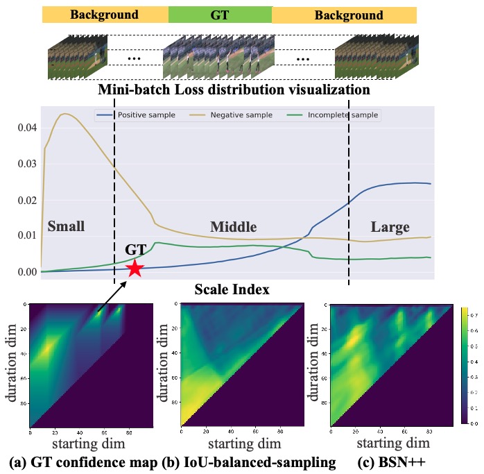
Figure 1: (a) Given an untrimmed video containing several action instances of small scale, (b) IoU-balanced sampling is widely used to train the proposal confidence regressor, which still suffers from inferior quality owing to the imbalanced distribution of the temporal durations, resulting in the long-tailed proposal dataset. (c) BSN++ aims at generating high-quality proposal boundaries as well as reliable confidence scores with complementary boundary regressor and scale-balanced proposal relation block.

Temporal action detection task has received much attention from many researchers in recent years, which requires not only categorizing the real-world untrimmed videos but also locating the temporal boundaries of action instances. Akin to object proposals for object detection in images, temporal action proposal indicates the temporal intervals containing the actions and plays an important role in temporal action detection. It has been commonly recognized that high-quality proposals usually have two crucial properties: (1) the generated proposals should cover the action instances temporally with both high recall and temporal overlapping; (2) the quality of proposals should be evaluated accurately, thus providing a overall confidence for later retrieving step.

To cater for these two conditions and achieve high quality proposals, there are two main categories in the existing proposal generation methods (Buch et al. 2017b; Gao et al. 2017; Lin, Zhao, and Shou 2017; Shou, Wang, and Chang 2016). The first type adopts the top-down fashion, where proposals are generated based on sliding windows (Shou, Wang, and Chang 2016) or uniform-distributed anchors (Lin, Zhao, and Shou 2017), then a binary classifier is employed to evaluate confidence for the proposals. However, the proposals generated in this way are doomed to have imprecise boundaries though with regression. Under this circumstance, the other type of methods (Lin et al. 2018; Xiong et al. 2017; Lin et al. 2019) attract many researchers recently which tackle this problem in a bottom-up fashion, where the input video is evaluated in a finer-level. (Lin et al. 2018) is a typical method in this type which proposes the Boundary-Sensitive Network (BSN) to generate proposals with flexible durations and reliable confidence scores. Though BSN achieves convincing performance, it still suffers from three main drawbacks: (1) BSN only employs the local details around the boundaries to predict boundaries, without taking advantage of the rich temporal contexts through the whole video sequence; (2) BSN fails to consider the proposal-proposal relations for confidence evaluation; (3) the imbalance data distribution between positive/negative proposals and temporal durations is also neglected.

To relieve these issues, we propose BSN++, for temporal proposal generation. (i) To exploit the rich contexts for boundary prediction, we adopt the U-shaped architecture with nested skip connections. Meanwhile, the two optimized boundary classifiers share the same goals especially in detecting the sudden change from background to actions or learning the discriminativeness from actions to background, thus are complementary with each other. Under this circumstance, we propose the complementary boundary regressor, where the starting classifier can also be used to predict the ending locations when the input videos are processed in a reversed direction, and vice versa. In this way, we can achieve high precision without adding extra parameters. (ii) In order to predict the confidence scores of densely-distributed proposals, we design a proposal relation block aiming at leveraging both channel-wise and position-wise global dependencies for proposal-proposal relation modeling. (iii) To relieve the imbalance scale-distribution among the sampling positives as well as the negatives (see Fig. 1), we implement a two-stage re-sampling scheme consisting of the IoU-balanced (positive-negative) sampling and the scale-balanced re-sampling. The boundary map and the confidence map are generated simultaneously and jointly trained in a unified framework. In summary, the main contributions of our work are listed below in three-folds:

• We revisit the boundary prediction problem and propose a complementary boundary generator to exploit both “local and global”, “past and future” contexts for accurate temporal boundary prediction.

• We propose a proposal relation block for proposal confidence evaluation, where two self-attention modules are adopted to model the proposal relations from two complementary aspects. Besides, we devise a two-stage re-sampling scheme for equivalent balancing.

• Thorough experiments are conducted to reveal the effectiveness of our method. Further combining with the existing action classifiers, our method can achieve the state-of-the-art temporal action detection performance.

Related Work

Action Recognition

Action recognition is an essential branch which has been extensively explored in recent years. Earlier methods such as improved Dense Trajectory (iDT) (Wang et al. 2011; Wang and Schmid 2013) mainly adopt the hand-crafted features including HOG, MBH and HOF. Current deep learning based methods (Feichtenhofer, Pinz, and Zisserman 2016; Simonyan and Zisserman 2014; Tran et al. 2015; Wang et al. 2016; Su et al. 2020a) typically contain two main categories: the two-stream networks (Feichtenhofer, Pinz, and Zisserman 2016; Simonyan and Zisserman 2014) capture the appearance and motion information from RGB image and stacked optical flow respectively; 3D networks (Tran et al. 2015; Qiu, Yao, and Tao 2017) exploit 3D convolutions to capture the spatial and temporal information directly from the raw videos. Action recognition networks are usually adopted to extract visual feature sequence from untrimmed videos for the temporal action proposals and detection task.

Imbalanced Distribution Training

Imbalanced data distribution naturally exists in many large-scale datasets (Cordt et al. 2018; Cordts et al. 2016; Feng et al. 2018). Current literature can be mainly divided into three categories: (1) re-sampling, includes oversampling the minority classes (Estabrooks, Jo, and Japkowicz 2004; Ji et al. 2020) or downsampling the majority classes (Weiss, McCarthy, and Zabar 2007; Hu et al. 2020); (2) re-weighting, namely cost sensitive learning (McCarthy, Zabar, and Weiss 2005; Cui et al. 2019), which aims to dynamically adjust the weight of samples or different classes during training process. (3) In object detection task, the imbalanced issue is more serious between background and foreground for one-stage detector. Some methods such as Focal loss (Lin et al. 2017) and online hard negative mining (Shrivastava, Gupta, and Girshick 2016) are designed for two-stage detector. In this paper, we implement the scale-balanced re-sampling upon the IoU-balanced sampling for proposal confidence evaluation, motivated by the mini-batch imbalanced loss distribution against proposal durations.

Temporal Action Detection and Proposals

Akin to object detection in images, temporal action detection also can be divided into proposal and classification stages. Current methods train these two stages separately (Singh and Cuzzolin 2016) or jointly (Buch et al. 2017a; Lin, Zhao, and Shou 2017). Top-down methods (Lin, Zhao, and Shou 2017) are mainly based on sliding windows or pre-defined anchors, while bottom-up methods (Xiong et al. 2017; Lin et al. 2018, 2019) first evaluate the actionness or boundary probabilities of each temporal location in a finer level. However, proposals generated in a local fashion of (Xiong et al. 2017) cannot be further retrieved without confidence scores evaluated from a global view. And probabilities sequence generated in (Lin et al. 2018, 2019; Liu et al. 2019) is sensitive to noises, causing many false alarms. Besides, proposal-proposal relations fail to be considered for confidence evaluation. Meanwhile, the imbalanced distribution among the proposals remains to be settled. To address these issues, we propose BSN++, which is unique to previous works in three main aspects: (1) we revisit the boundary prediction task and propose to exploit rich contexts together with bi-directional matching strategy for accurate boundary prediction; (2) we devise a proposal relation block for proposal-proposal relations modeling; (3) two-stage re-sampling scheme is designed for equivalent balancing.

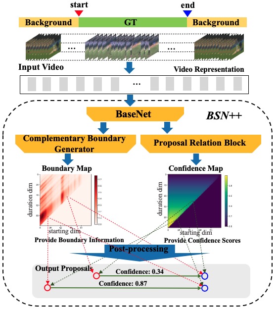
Figure 2: The framework of BSN++. Given an untrimmed video, two-stream network is adopted to extract visual features. Then BSN++ can densely evaluate all proposals by producing the boundary map with a complementary boundary generator and the confidence map with a proposal relation block simultaneously.

Our Approach

Problem Definition

Denote an untrimmed video sequence as $\mathbf{U}=\{\mathbf{u}_{t}\}_{t=1}^{l_{v}},$ where $\mathbf{u}_{t}$ indicates the $t$-th frame in the video of length $l_{v}$. A set of action instances $\mathbf{\Psi}_{g}=\{\mathbf{\varphi}_{n}=(t_{n}^{s},t_{n}^{e})\}_{n=1}^{N_{g}}$ are temporally annotated in the video $\mathbf{S}_{v}$, where $N_{g}$ is the number of ground truth action instances, and $t_{n}^{s},t_{n}^{e}$ are the starting time and ending time of the action instance $\varphi_{n}$ respectively. During training phase, the $\mathbf{\Psi}_{g}$ is provided. While in the testing phase, the predicted proposal set $\mathbf{\Psi}_{p}$ should cover the $\mathbf{\Psi}_{g}$ with high recall and high temporal overlapping.

Video Feature Encoding

Before applying our algorithm, we adopt the two-stream network (Simonyan and Zisserman 2014) in advance to encode the visual features from raw video as many previous works (Lin et al. 2018; Gao, Kan, and Nevatia 2018; Su, Zhao, and Lin 2018; Su et al. 2020b). This kind of architecture has been widely used in many video analysis tasks(Lin, Zhao, and Shou 2017; Zhao et al. 2017; Gao, Yang, and Nevatia 2017). Concretely, given an untrimmed video $\mathbf{S}_{v}$ which contains $l_{v}$ frames, we process the input video in a regular interval $\sigma$ for reducing the computational cost. We concatenate the output of the last FC-layer in the two-stream network to form the feature sequence $\mathbf{F}=\{\mathbf{f}_{i}\}_{i=1}^{l_{s}}$, where $l_{s}=l_{v}/\sigma$. Final, the feature sequence $\mathbf{F}$ is used as the input of our BSN++.

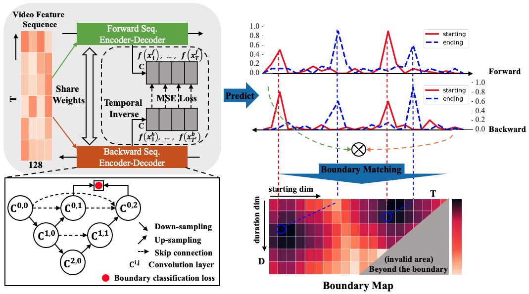
Figure 3: Illustration of the complementary boundary generator. U-shaped encoder-decoder with dense skip connections are utilized for accurate boundary prediction. Consistent regularization is performed on the intermediate features during the training process. In inference stage, starting/ending classifiers are also utilized to predict the ending/starting locations in a backward order. The two siamese backbones share the weights. Finally the boundary map is constructed through matching boundary locations into pairs based on the two-passes boundary probabilities sequence.

Proposed Network Architecture: BSN++

In contrast to the previous BSN (Lin et al. 2018), which consists of multiple stages, BSN++ is designed to generate the proposal map directly in a unified network. To obtain the proposal map, BSN++ first generates the boundary map which represents the boundary information and confidence map which represents the confidence scores of densely distributed proposals. As shown in Fig. 2, BSN++ model mainly contains three main modules: Base Module handles the input video features to perform temporal information modeling, then the output features are shared by the two following modules. Complementary Boundary Generator processes the input video features to evaluate the boundary probabilities sequence, using a nested U-shaped encoder-decoder; Proposal Relation Block aims to model the proposal-proposal relations with two self-attention modules responsible for two complementary dependencies.

Base Module. The goal of this module is to handle the extracted features for temporal relationship modeling, which serves as the base module of the following two branches. It mainly includes two 1D convolutional layers, with 256 filters, kernel size 3 and stride 1, followed by a ReLU activation layer. Since the length of videos is uncertain, we truncate the video sequence into a series of sliding windows. The detailed of data construction is illustrated in Section 4.1.

Complementary Boundary Generator. Inspired by the success of U-Net (Ronneberger, Fischer, and Brox 2015; Zhou et al. 2018) used in image segmentation, we design our boundary generator as Encoder-Decoder networks because this kind of architecture is able to capture both high-level global context and low-level local details at the same time. As shown in Fig. 3, each circle represents a 1D convolutional layer with 512 filters and kernel size 3, stride 1, together with a batch normalization layer and a ReLU layer except the prediction layer. To reduce over-fitting, we just add two down-sampling layers to expand the receptive fields and the same number of up-sampling layers are followed to recover the original temporal resolutions. Besides, deep supervision (shown red) is also performed for fast convergent speed and nested skip connections are employed for bridging the semantic gap between feature maps of the encoder and decoder prior to fusion.

We observe that the starting classifier learns to detect the sudden change from background to actions and vice versa. Hence, the starting classifier can be regarded as a pseudo ending classifier when processes the input video in a reversed direction, thus the bi-directional prediction results are complementary. With this observation, bi-directional encoder-decoder networks are optimized in parallel, and the consistent constraint is performed upon the intermediate features (i.e. $f(x^{f}_{i})$ and $f(x^{b}_{i})$) on both sides before the prediction layer as shown in Fig. 3. During the inference stage, the aforementioned encoder-decoder network is adopted to predict the the starting heatmap $\overrightarrow{\mathbf{H}}^{s}=\{\overrightarrow{\mathbf{h}}_{i}^{s}\}_{i=1}^{l_{s}}$ and ending heatmap $\overrightarrow{\mathbf{H}}^{e}=\{\overrightarrow{\mathbf{h}}_{i}^{e}\}_{i=1}^{l_{s}}$ respectively, where $\mathbf{h}_{i}^{s}$ and $\mathbf{h}_{i}^{e}$ indicate the starting and ending probabilities of the $i$-th snippet respectively. Meanwhile, we feed the input feature sequence in a reversed order to the identical backbone. Similarly, we can obtain the starting heatmap $\overleftarrow{\mathbf{H}}^{s}$ and ending heatmap $\overleftarrow{\mathbf{H}}^{e}$.

After the two-passes, in order to select the boundaries of high scores, we fuse the two pairs of heatmaps to yield the final heatmaps:

$$\mathbf{H}^{s}=\{\sqrt{\overrightarrow{\mathbf{h}_{i}^{s}}\times\overleftarrow{\mathbf{h}}_{i}^{s}}\}_{i=1}^{l_{s}},\mathbf{H}^{e}=\{\sqrt{\overrightarrow{\mathbf{h}}_{i}^{e}\times\overleftarrow{\mathbf{h}}_{i}^{e}}\}_{i=1}^{l_{s}},$$ (1)

With these two boundary points heatmaps, we can further construct the boundary map $\mathbf{M}^{b}\in R^{1\times D\times T}$ which can represent the boundary information of all densely distributed proposals, where $T$ and $D$ are the length of the feature sequence and maximum duration of proposals separately:

$$\mathbf{M}_{j,i}^{b}=\{\{\mathbf{h}_{i}^{s}\times\mathbf{h}_{i+j}^{e}\}_{i=1}^{T}\}_{j=1}^{D},i+j<T,$$ (2)

Proposal Relation Block. The goal of this block is to evaluate the confidence scores of dense proposals. Before performing proposal-proposal relations, we follow the previous work BMN (Lin et al. 2019) to generate the proposal feature maps as $\mathbf{F}^{p}\in R^{D\times T\times 128\times N}$. N is set to 32. Then the proposal feature maps are fed to a 3D convolutional layer with kernel size $1\times 1\times 32$ and 512 filters, followed by a ReLU activation layer. Thus the reduced proposal features maps are $\widehat{\mathbf{F}^{p}}\in R^{D\times T\times 512}$. The proposal relation block consists of two self-attention modules as follows.

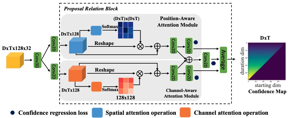
Figure 4: Illustration of the proposal relation block. After generating the proposal feature maps, two complementary branches are followed to model the proposal relation separately. In the upper branch, the position-aware attention module aims to leverage global dependencies. While in the lower branch, the channel-aware attention module aims to attend to the discriminative features by channel matrix calculation. Finally, we aggregate the outputs from the three branches for pixel-level confidence prediction.

Position-aware attention module. As illustrated in Fig. 4, given the proposal features $\widehat{\mathbf{F}^{p}}$, we adopt the similar self-attention mechanism as (Wang et al. 2018), where the proposal feature maps are fed into a convolutional layer separately to generate two new feature maps $A$ and $B$ for spatial matrix multiplication with reshape and transpose operations. And then a Softmax layer is applied to calculate the position-aware attention $P^{A}\in R^{L\times L}$, where $L=D\times T$:

$$P^{A}_{j,i}=\dfrac{\exp(A_{i}\cdot B_{j})}{\sum_{i=1}^{L}\exp(A_{i}\cdot B_{j})},$$ (3)

where $P^{A}_{j,i}$ indicates the attention of the $i^{th}$ position on the $j^{th}$ position. Finally, the attended features are further weighted summed with the proposal features and fed to the convolutional layers for confidence prediction.

Channel-aware attention module. In contrast to the position-aware attention module, this module directly performs channel-wise matrix multiplication in order to exploit the inter-dependencies among different channels, which can help enhance the proposal feature representations for confidence prediction. The process of attention calculation is the same as the former module except for the attended dimension. Similarly, the attended features after weighted summed with the proposal features are further captured by a 2D convolutional layer to generate the confidence map $\mathbf{M}^{c}\in R^{D\times T}$. We also aggregate the outputs of the two attention modules for proposal confidence prediction, and finally we fuse the predicted confidence maps from the three branches for a better performance.

Re-sampling

Imbalanced data distribution can affect the model training especially in the long-tailed dataset. In this paper, we revisit the positive/negative samples distribution for improving the quality of proposal confidence prediction and design a proposal-level re-sampling method to improve the performance of training on the long-tailed dataset. Our re-sampling scheme consists of two stages aiming at not only balancing the positives and negatives proposals, but also balancing the temporal duration of the proposals.

IoU-balanced sampling

As shown in Fig. 1, we can see from the mini-batch loss distribution that the number of positives and negatives differs greatly which dooms to bias the training model without effective measures. Previous works usually design a positive-negative sampler (i.e. IoU-balanced sampler) to balance the data distribution for each mini-batch, thus ensuring the ratio of positive and negative samples is nearly 1:1. However, we can also conclude from the Fig. 1 that the scale of positives or negatives fails to conform the uniform distribution. Under this circumstance, we should consider how to balance the scales of proposals.

Scale-balanced re-sampling

To relieve the issue among long-tailed scales, we propose a second-stage positive/negative re-sampling method, which is upon the principle of IoU-balanced sampling. Specifically, define $P_{i}$ as the number of positive proposals with the scale $s_{i}$, then $r_{i}$ is the positive ratio of $s_{i}$:

$$\begin{split}&r_{i}=\dfrac{P_{i}}{\sum_{j=1}^{N_{s}}P_{j}},\\ &r^{{}^{\prime}}_{i}=\left\{\begin{aligned} &\lambda\ast exp^{(\dfrac{r_{i}}{\lambda}-1)}\quad&(0<r_{i}\leq\lambda),\\ &r_{i}\quad&(\lambda<r_{i}\leq 1),\end{aligned}\right.\end{split}$$ (4)

where $N_{s}$ is the number of pre-defined normalized scale regions (i.e. $[0-0.3,0.3-0.7,0.7-1.0]$). Then we design a positive ratio sampling function, the resulting ratio $r^{{}^{\prime}}_{i}$ is bigger than $r_{i}$ for proposal scale with a frequency lower than $\lambda$, where $\lambda$ is a hyper-parameter which we set to 0.15 empirically. Hence, we use the re-normalized $r^{{}^{\prime}}_{i}$ as the sampling probability of the specific proposal scale region $s_{i}$ to construct the mini-batch data. As for the negative proposals, the same process is performed.

Training and Inference of BSN++

Training

Overall Objective Function. As described above, BSN++ consists of three main sub-modules. The multi-task objective function is defined as:

$$L_{BSN++}=L_{CBG}+\beta\cdot L_{PRB}+\gamma\cdot L_{2}(\Theta),$$ (5)

where $L_{CBG}$ and $L_{PRB}$ are the objective functions of the complementary boundary generator and the proposal relation block respectively, while $L_{2}(\Theta)$ is a regularization term. $\beta$ and $\gamma$ are set to 10 and 0.0001 separately to trade off the training process of two modules and reduce over-fitting.

Training Data Construction. Given the extracted feature $\mathbf{F}$ with length $l_{s}$, we truncate $\mathbf{F}$ into sliding windows of length $l_{w}$ with 75% temporal overlapping. Then we construct the training dataset as $\Phi=\{\mathbf{F}^{w}_{n}\}_{n=1}^{N_{w}}$, where $N_{w}$ is the number of retained windows containing at least one ground-truth.

Label Assignment. For the Complementary Boundary Generator (CBG), in order to predict the boundary probabilities sequence, we need to generate the corresponding label sequence $\mathbf{G}_{s}^{w}$ and $\mathbf{G}_{e}^{w}$ as in (Lin et al. 2018). Specifically, for each action instance $\varphi_{g}$ in the annotation set $\mathbf{\Psi}_{g}^{w}$, we denote it’s starting and ending regions as $[t_{g}^{s}-d_{\varphi}/10,t_{g}^{s}+d_{\varphi}/10]$ and $[t_{g}^{e}-d_{\varphi}/10,t_{g}^{e}+d_{\varphi}/10]$ respectively, where $d_{\varphi}=t_{g}^{e}-t_{g}^{s}$ is the duration of $\varphi_{g}$. Then for each temporal location, if it lies in the starting or ending regions of any action instances, the corresponding label $\mathbf{g}^{s}$ or $\mathbf{g}^{e}$ will be set to 1. Hence the label sequence of starting and ending used in CBG are $\mathbf{G}_{s}^{w}=\{\mathbf{g}_{i}^{s}\}_{i=1}^{l_{w}}$, $\mathbf{G}_{e}^{w}=\{\mathbf{g}_{i}^{e}\}_{i=1}^{l_{w}}$ respectively.

For the Proposal Relation Block (PRB), we predict the confidence map $\mathbf{M}^{c}\in R^{D\times l_{w}}$ of all densely distributed proposals, where the point $g^{c}_{j,i}$ in the label confidence map $\mathbf{M}_{g}^{c}=\{\{g^{c}_{j,i}\}_{i=1}^{l_{w}}\}_{j=1}^{D}$ represents the maximum $IoU$ (Intersection-over-Union) values of proposal $\varphi_{j,i}=[t_{s}=i,t_{e}=i+j]$ with all $\varphi_{g}$ in $\mathbf{\Psi}_{g}^{w}$.

Objective of CBG. We follow (Lin et al. 2018) to adopt the weighted binary logistic regression loss $L_{bl}$ as the objective between the output probability and the corresponding label sequence. The objective is:

$$L_{CBG}=\underbrace{\overrightarrow{L_{bl}^{s}}+\overrightarrow{L_{bl}^{e}}}_{forward}+\underbrace{\overleftarrow{L_{bl}^{s}}+\overleftarrow{L_{bl}^{e}}}_{backward}+||f(x^{f})-f(x^{b})||^{2},$$ (6)

where $\overrightarrow{L_{bl}^{s}}$ and $\overrightarrow{L_{bl}^{e}}$ represent the $L_{bl}$ between $\overrightarrow{\mathbf{H}}^{s}$ and $\mathbf{G}_{s}^{w}$, $\overrightarrow{\mathbf{H}}^{e}$ and $\mathbf{G}_{E}^{w}$ respectively in the forward pass. Mean-Squared Loss is also performed on two-passes intermediate features.

Objective of PRB. Taking the constructed proposal feature maps $\mathbf{F}^{p}$ as input, our PRB will generate two types of confidence maps $\mathbf{M}^{cr}$ and $\mathbf{M}^{cc}$ for all densely distributed proposals as (Lin et al. 2019). The training objective is defined as the regression loss $L_{reg}$ and the binary classification loss $L_{cls}$ respectively:

$$L_{PRB}=L_{reg}+L_{cls},$$ (7)

where the smooth-$L_{1}$ loss (Girshick 2015) is adopted as $L_{reg}$, and the points $g^{c}_{i,j}$ with value large than 0.7 or lower than 0.3 are regarded as positives and negatives respectively. And we ensure the scale and number ratio between positives and negatives to be near 1:1 by the two-stage sampling scheme described above.

Inference

During inference stage, our BSN++ can generate the boundary map $\mathbf{M}^{b}$ based on the bidirectional boundary probabilities ($\mathbf{H}^{s}$ and $\mathbf{H}^{e}$) and confidence map ($\mathbf{M}^{cc}$ and $\mathbf{M}^{cr}$). We form the proposal map $\mathbf{M}^{p}$ directly by fusing the $\mathbf{M}^{b}$ and $\mathbf{M}^{c}$ with dot multiplication. Then we can filter the points with high scores in the proposal map $\mathbf{M}^{p}$ as candidate proposals used for post-processing.

Score Fusion. As described above, the final scores of proposals in $\mathbf{M}^{p}$ involve the local boundary information and global confidence scores. Take the proposal $\varphi$ = $[t_{s},t_{e}]$ for example, the combination of final score $p_{\varphi}$ can be shown as:

$$p_{\varphi} =\mathbf{M}^{b}_{t_{e}-t_{s},t_{s}}\cdot\sqrt{\mathbf{M}^{cc}_{t_{e}-t_{s},t_{s}}\cdot\mathbf{M}^{cr}_{t_{e}-t_{s},t_{s}}},$$ (8)

Redundant Proposals Suppression. BSN++ can generate the proposal candidates set as $\mathbf{\Psi}_{p}=\{\varphi_{n}=(t_{s},t_{e},p_{\varphi})\}_{n=1}^{N_{p}}$, where $N_{p}$ is the number of proposals. Since the generated proposals may overlap with each other, we conduct Soft-NMS (Bodla et al. 2017) algorithm to suppress the confidence scores of redundant proposals. Final, the proposals set is $\mathbf{\Psi}_{p}^{\prime}=\{\varphi_{n}^{{}^{\prime}}=(t_{s},t_{e},p_{\varphi}^{{}^{\prime}})\}_{n=1}^{N_{p}}$, where $p_{\varphi}^{{}^{\prime}}$ is the decayed score of proposal $\varphi_{n}^{{}^{\prime}}$.

Experiments

Datasets and Setup

Datasets. ActivityNet-1.3 (Caba Heilbron et al. 2015) is a large-scale video dataset for action recognition and temporal action detection tasks used in the ActivityNet Challenge from 2016 to 2020. It contains 19, 994 videos with 200 action classes temporally annotated, and the ratio of training, validation and testing sets is 1:1:2. THUMOS-14 (Jiang et al. 2014) contains 200 and 213 untrimmed videos with temporal annotations of 20 action classes in validation and testing sets respectively.

Implementation details. For feature encoding, we adopt the two-stream network (Simonyan and Zisserman 2014), where ResNet network (He et al. 2016) and BN-Inception network (Ioffe and Szegedy 2015) are used as the spatial and temporal networks respectively. During feature extraction, the interval $\sigma$ is set to 16 and 5 on ActivityNet-1.3 and THUMOS14 respectively. On ActivityNet-1.3, we rescale the feature sequence of input videos to $l_{w}=100$ by linear interpolation following (Lin et al. 2018), and the maximum duration $D$ is also set to 100 to cover all action instances. While on THUMOS14, the length $l_{w}$ of sliding windows is set to 128 while the maximum duration $D$ is set to 64, which can cover almost 98% action instances. On both datasets, we train our BSN++ from scratch using the Adam optimizer and the batch size is set to 16. And the initial learning rate is set to 0.001 for 7 epochs, then 0.0001 for another 3 epochs.

Temporal Proposal Generation

Evaluation metrics. Following the conventions, Average Recall (AR) is calculated under different tIoU thresholds which are set to [0.5:0.05:0.95] on ActivityNet-1.3, and [0.5:0.05:1.0] on THUMOS14. We measure the relation between AR and Average Number (AN) of proposals, denoted as AR@AN. And we also calculate the area (AUC) under the AR vs. AN curve as another evaluation metric on ActivityNet-1.3 dataset, where AN ranges from 0 to 100.

Comparison to the state-of-the-arts. Table 1 illustrates the comparison results on ActivityNet-1.3. It can be observed that our BSN++ outperforms other state-of-the-art proposal generation methods with a big margin in terms of AR@AN and AUC on validation set of ActivityNet-1.3. For a direct comparison to BSN, our BSN++ improves AUC from 66.17% to 68.26% on validation set. Particularly, when the AN is 100, our method significantly improves AR from 74.16% to 76.52% by 2.36%. And when the AN is 1, the AR which our BSN++ can obtain is 34.30%.

Table 2 illustrates the comparison results on THUMOS14 dataset. For fair comparisons, we use the features when compared with other methods, which mainly includes two-stream features and C3D features (Tran et al. 2015). Results shown in Table 2 clearly demonstrate that: (1) the performance of our BSN++ obviously outperforms other state-of-the-methods in terms of AR@AN with AN varying from 50 to 1000, no matter what kind of features is served as input; (2) when post-processed with Soft-NMS, the higher AR can be obtained with fewer proposals. Qualitative examples on THUMOS14 and ActivityNet-1.3 are shown in Fig. 5.

Table 1: Performance comparisons with other state-of-the-art proposal generation methods on validation set of ActivityNet-1.3 in terms of AUC and AR@AN.

Method	SSAD-prop	CTAP	BSN	MGG	BMN	BSN++
AR@1 (val)	-	-	32.17	-	-	34.30
AR@100 (val)	73.01	73.17	74.16	74.54	75.01	76.52
AUC (val)	64.40	65.72	66.17	66.43	67.10	68.26

Table 2: Comparisons with other state-of-the-art proposal generation methods SCNN-prop(Shou, Wang, and Chang 2016), SST(Buch et al. 2017b), TURN(Gao et al. 2017), MGG(Liu et al. 2019), BSN(Lin et al. 2018), BMN(Lin et al. 2019) on THUMOS14 in terms of AR@AN, where SNMS stands for Soft-NMS.

Feature	Method	@50	@100	@200	@500	@1000
C3D	TURN	19.63	27.96	38.34	53.52	60.75
C3D	MGG	29.11	36.31	44.32	54.95	60.98
C3D	BSN(SNMS)	29.58	37.38	45.55	54.67	59.48
C3D	BMN(SNMS)	32.73	40.68	47.86	56.42	60.44
C3D	BSN++(SNMS)	34.88	43.72	50.12	58.88	61.39
2-Stream	CTAP	32.49	42.61	51.97	-	-
2-Stream	MGG	39.93	47.75	54.65	61.36	64.06
2-Stream	BSN(SNMS)	37.46	46.06	53.21	60.64	64.52
2-Stream	BMN(SNMS)	39.36	47.72	54.70	62.07	65.49
2-Stream	Ours(SNMS)	42.44	49.84	57.61	65.17	66.83

Table 3: Ablation experiments in the validation set of ActivityNet-1.3. Complementary boundary generator is abbreviated as CBG and BBM denotes bi-directional matching. PRB is the proposal relation block and SBS is the scale-balanced sampling. PAM and CAM indicate the two self-attention modules. Inference speed here is the seconds (s) cost $T_{cost}$ for processing a 3-minute videos using a Nvidia 1080-Ti card. e2e denotes the joint training manner.

Model	Module	e2e	AUC	$T_{cost}$
BSN	TEM	-	64.80	0.036
BSN	TEM+PEM	$\times$	66.17	0.629
BMN	TEM	-	65.17	0.035
BMN	TEM+PEM	$\checkmark$	67.10	0.052
BSN++	CBG(w/o BBM)	-	66.02	0.019
BSN++	CBG(w/ BBM)	-	66.43	0.025
BSN++	CBG+PRB (w/o SBS)	$\times$	67.34	0.054
BSN++	CBG+PRB (w/o SBS)	$\checkmark$	67.77	0.039
BSN++	CBG+PRB (w/o PAM)	$\checkmark$	67.99	0.034
BSN++	CBG+PRB (w/o CAM)	$\checkmark$	68.01	0.035
BSN++	CBG+PRB	$\checkmark$	68.26	0.039

Table 4: Generalizability evaluation on ActivityNet-1.3.

BMN/BSN++	Seen(validation)		Unseen(validation)
Train Data	AR@100	AUC	AR@100	AUC
Seen+Unseen	72.96/74.56	65.02/66.34	72.68/74.32	65.06/66.37
Seen	72.47/74.03	64.37/65.87	72.46/73.82	64.47/65.89

Table 5: Detection results compared with (Zhao et al. 2017; Lin, Zhao, and Shou 2017; Lin et al. 2018, 2019; Zeng et al. 2019; Xu et al. 2020) on validation set of ActivityNet-1.3, where our proposals are combined with video-level classification results generated by (Xiong et al. 2016).

ActivityNet-1.3, mAP@$tIoU$
	validation
Method	0.5	0.75	0.95	Average
SSN	39.12	23.48	5.49	23.98
SSAD	44.39	29.65	7.09	29.17
BSN	46.45	29.96	8.02	30.03
P-GCN	48.26	33.16	3.27	31.11
BMN	50.07	34.78	8.29	33.85
G-TAD	50.36	34.60	9.02	34.09
Ours	51.27	35.70	8.33	34.88

Table 6: Detection results compared with (Gao et al. 2017; Lin et al. 2018; Liu et al. 2019; Lin et al. 2019) on testing set of THUMOS14, where video-level classifier (Wang et al. 2017) is combined with proposals generated by BSN++.

THUMOS14 (testing), mAP@$tIoU$
Method	Classifier	0.7	0.6	0.5	0.4	0.3
TURN	UNet	6.3	14.1	24.5	35.3	46.3
BSN	UNet	20.0	28.4	36.9	45.0	53.5
MGG	UNet	21.3	29.5	37.4	46.8	53.9
BMN	UNet	20.5	29.7	38.8	47.4	56.0
Ours	UNet	22.8	31.9	41.3	49.5	59.9

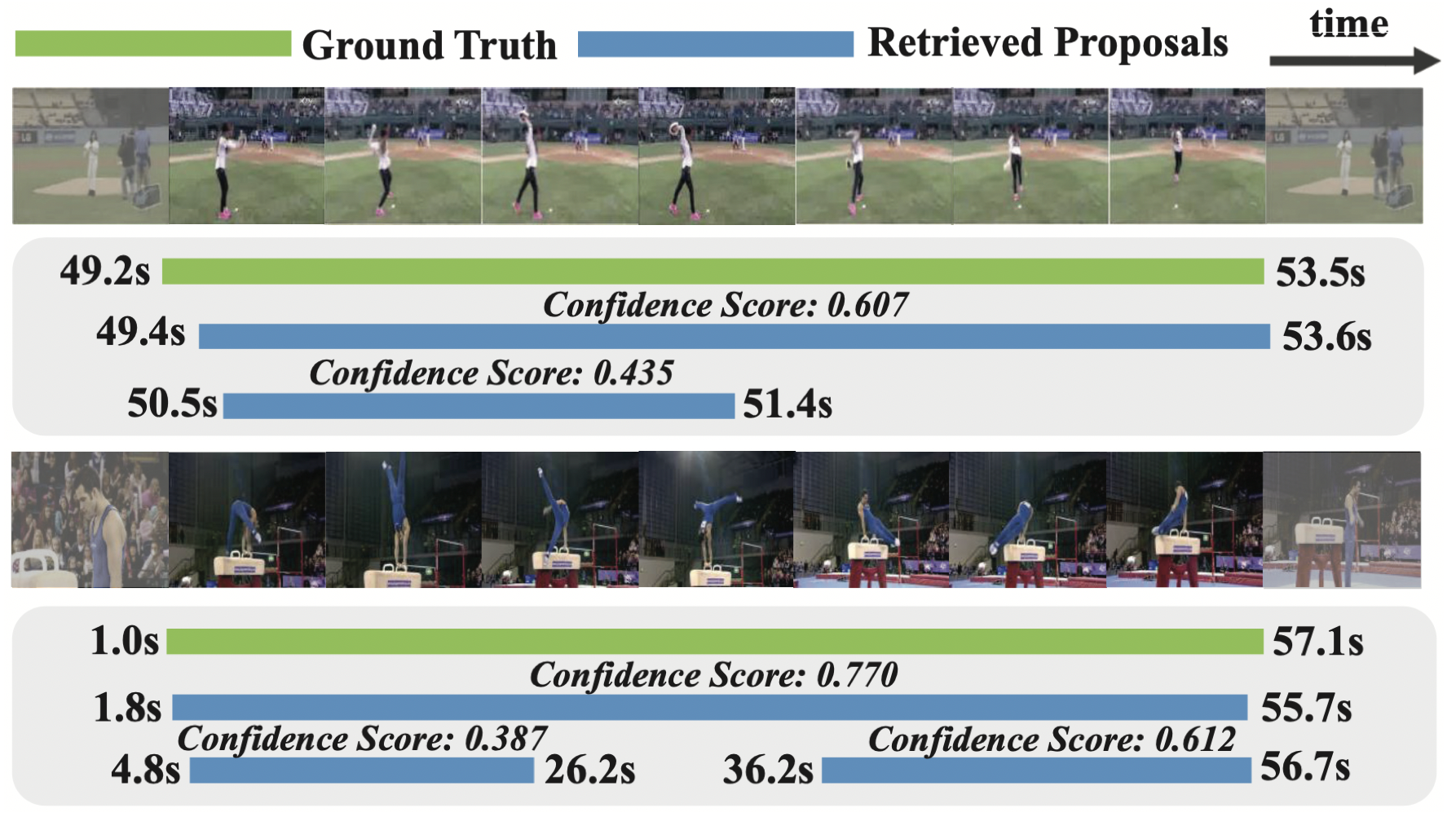
Figure 5: Qualitative examples of proposals generated by BSN++ on THUMOS14 (top) and ActivityNet-1.3 (bottom).

Ablation Experiments

In this section, we comprehensively evaluate our proposed BSN++ on the validation set of ActivityNet-1.3.

Effectiveness and efficiency of modules in BSN++. We perform the ablation studies with different architecture settings to verify the effectiveness and efficiency of each module proposed in BSN++. The evaluation results shown in Table 3 demonstrate that: (1) the Encoder-Decoder architecture can effectively learn “local and global” contexts for accurate boundary prediction compared to the previous works which only explore the local details; (2) the bidirectional matching mechanism further validates the importance of future context in assisting the boundary judgement; (3) unlike the previous works which treat the proposals separately, the proposal relation block can provide more comprehensive features for accurate and discriminative proposals scoring; (4) besides, with scale-balanced sampling, the model can obtain equivalent balancing; (5) final, integrating all the separated modules into an end-to-end network, we can obtain the competing performance improvement; (6) BSN++ achieves the great overall efficiency than previous methods.

Ablation comparison with BSN. We conduct a direct comparison to BSN(Lin et al. 2018) to confirm the effectiveness and superiority of our BSN++. As shown in Table 3, the TEM of BSN which only considers the local details for boundary probabilities sequence generation is inferior with limited receptive fields. Meanwhile, without the full usage of temporal context, it is also not robust in complicated scenarios. Besides, BSN fails to model the proposal relations for confidence regression, as well as neglect the imbalance data distribution against proposal duration. However, our BSN++ handles these issues accordingly and effectively.

Generalizability of proposals. Another key property of the proposal generation method is the generalizability. To evaluate this property, two un-overlapped action subsets: “Sports, Exercise, and Recreation” and “Socializing, Relaxing, and Leisure” of ActivityNet-1.3 are chosen as seen and unseen subsets separately. There are 87 and 38 action categories, 4455 and 1903 training videos, 2198 and 896 validation videos on seen and unseen subsets separately. We adopt C3D network pre-trained on Sports-1M dataset for feature extraction. Then we train BSN++ with seen and seen+unseen training videos separately, and evaluate both models on seen and unseen validation videos separately. Results in Table 4 reveal that there is only slight performance drop on unseen categories, suggesting that BSN++ achieves great generalizability to generate high quality proposals for unseen actions.

Action Detection with Our Proposals

Evaluation metrics. For temporal action detection task, mean Average Precision (mAP) is a conventional evaluation metric, where Average Precision (AP) is calculated for each action category respectively. On ActivityNet-1.3, the mAP with tIoU thresholds set $\{0.5,0.75,0.95\}$ and the average mAP with tIoU thresholds [0.5:0.05:0.95] are reported. On THUMOS14, mAP with tIoU thresholds set $\{0.3,0.4,0.5,0.6,0.7\}$ is used.

Comparison to the state-of-the-arts. To further examine the quality of proposals generated by BSN++, following BSN(Lin et al. 2018), we feed them to the state-of-the-art action classifiers to obtain the categories for action detection in a “detection by classification” framework. On ActivityNet-1.3, we use the top-1 video-level classification results generated by (Xiong et al. 2016) for all the generated proposals. And on THUMOS14, we use the top-2 video-level classification results generated by UntrimmedNet (Wang et al. 2017). Comparison results are illustrated in Table 5 and Table 6 respectively. We can observe that with the same classifiers, the detection performance of our method can be boosted greatly, which can further demonstrate the effectiveness and superiority of our method.

Conclusion

We propose BSN++ for temporal action proposal generation. The complementary boundary generator takes the advantage of U-shaped architecture and bi-directional boundary matching mechanism to learn rich contexts for boundary prediction. To model the proposal-proposal relations for confidence evaluation, we devise the proposal relation block which employs two self-attention modules to perform global and inter-dependencies modeling. Meanwhile, we are the first to consider the imbalanced data distribution of proposal durations. Both the boundary map and confidence map can be generated simultaneously in a unified network. Extensive experiments conducted on ActivityNet-1.3 and THUMOS14 datasets demonstrate the effectiveness of our method in both temporal action proposal and detection performance.

References

- Bodla et al. (2017) Bodla, N.; Singh, B.; Chellappa, R.; and Davis, L. S. 2017. Improving Object Detection With One Line of Code. In arXiv preprint arXiv:1704.04503.
- Buch et al. (2017a) Buch, S.; Escorcia, V.; Ghanem, B.; Fei-Fei, L.; and Niebles, J. C. 2017a. End-to-End, Single-Stream Temporal Action Detection in Untrimmed Videos. In Proceedings of the British Machine Vision Conference.
- Buch et al. (2017b) Buch, S.; Escorcia, V.; Shen, C.; Ghanem, B.; and Niebles, J. C. 2017b. Sst: Single-stream temporal action proposals. In CVPR, 6373–6382. IEEE.
- Caba Heilbron et al. (2015) Caba Heilbron, F.; Escorcia, V.; Ghanem, B.; and Carlos Niebles, J. 2015. Activitynet: A large-scale video benchmark for human activity understanding. In CVPR, 961–970.
- Cordt et al. (2018) Cordt, M.; Omran, M.; Ramos, S.; Rehfeld, T.; Enzweiler, M.; Benenson, R.; Franke, U.; Roth, S.; and Schiele, B. 2018. The open images dataset v4: Unified image classification, object detec- tion, and visual relationship detection at scale. arXiv preprint arXiv:1811.00982, 2018 .
- Cordts et al. (2016) Cordts, M.; Omran, M.; Ramos, S.; Rehfeld, T.; Enzweile, M.; and Schiele, B. 2016. The cityscapes dataset for semantic urban scene understanding. CVPR .
- Cui et al. (2019) Cui, Y.; Jia, M.; Lin, T.-Y.; Song, Y.; and Belongie, S. 2019. Class-balanced loss based on effective number of samples. CVPR .
- Estabrooks, Jo, and Japkowicz (2004) Estabrooks, A.; Jo, T.; and Japkowicz, N. 2004. A multiple resampling method for learning from imbalanced data sets. Computational intelligence .
- Feichtenhofer, Pinz, and Zisserman (2016) Feichtenhofer, C.; Pinz, A.; and Zisserman, A. 2016. Convolutional two-stream network fusion for video action recognition. In CVPR, 1933–1941.
- Feng et al. (2018) Feng, W.; Ji, D.; Wang, Y.; Chang, S.; Ren, H.; and Gan, W. 2018. Challenges on Large Scale Surveillance Video Analysis. In Proceedings of the IEEE Conference on Computer Vision and Pattern Recognition (CVPR) Workshops.
- Gao, Kan, and Nevatia (2018) Gao, J.; Kan, C.; and Nevatia, R. 2018. CTAP: Complementary Temporal Action Proposal Generation. arXiv preprint arXiv:1807.04821 .
- Gao, Yang, and Nevatia (2017) Gao, J.; Yang, Z.; and Nevatia, R. 2017. Cascaded boundary regression for temporal action detection. arXiv preprint arXiv:1705.01180 .
- Gao et al. (2017) Gao, J.; Yang, Z.; Sun, C.; Chen, K.; and Nevatia, R. 2017. TURN TAP: Temporal Unit Regression Network for Temporal Action Proposals. In ICCV, 3648–3656. IEEE.
- Girshick (2015) Girshick, R. 2015. Fast r-cnn. In ICCV, 1440–1448.
- He et al. (2016) He, K.; Zhang, X.; Ren, S.; and Sun, J. 2016. Deep residual learning for image recognition. In CVPR, 770–778.
- Hu et al. (2020) Hu, H.; Ji, D.; Gan, W.; Bai, S.; Wu, W.; and Yan, J. 2020. Class-wise Dynamic Graph Convolution for Semantic Segmentation. arXiv preprint arXiv:2007.09690 .
- Ioffe and Szegedy (2015) Ioffe, S.; and Szegedy, C. 2015. Batch normalization: Accelerating deep network training by reducing internal covariate shift. arXiv preprint arXiv:1502.03167 .
- Ji et al. (2020) Ji, D.; Wang, H.; Hu, H.; Gan, W.; Wu, W.; and Yan, J. 2020. Context-Aware Graph Convolution Network for Target Re-identification. arXiv preprint arXiv:2012.04298 .
- Jiang et al. (2014) Jiang, Y.; Liu, J.; Zamir, A. R.; Toderici, G.; Laptev, I.; Shah, M.; and Sukthankar, R. 2014. THUMOS challenge: Action recognition with a large number of classes. In Computer Vision-ECCV workshop 2014.
- Lin et al. (2019) Lin, T.; Liu, X.; Li, X.; Ding, E.; and Wen, S. 2019. BMN: Boundary-Matching Network for Temporal Action Proposal Generation. CoRR abs/1907.09702 .
- Lin, Zhao, and Shou (2017) Lin, T.; Zhao, X.; and Shou, Z. 2017. Single shot temporal action detection. In Proceedings of the 2017 ACM on Multimedia Conference, 988–996. ACM.
- Lin et al. (2018) Lin, T.; Zhao, X.; Su, H.; Wang, C.; and Yang, M. 2018. BSN: Boundary Sensitive Network for Temporal Action Proposal Generation. arXiv preprint arXiv:1806.02964 .
- Lin et al. (2017) Lin, T.-Y.; Goyal, P.; Girshick, R.; He, K.; and Dollar, P. 2017. Focal loss for dense object detection. ICCV .
- Liu et al. (2019) Liu, Y.; Ma, L.; Zhang, Y.; Liu, W.; and Chang, S.-F. 2019. Multi-granularity Generator for Temporal Action Proposal. In CVPR, 3604–3613.
- McCarthy, Zabar, and Weiss (2005) McCarthy, K.; Zabar, B.; and Weiss, G. 2005. Does cost- sensitive learning beat sampling for classifying rare classes? Proceedings ofthe 1st international workshop on Utility- based data mining .
- Qiu, Yao, and Tao (2017) Qiu, Z.; Yao, T.; and Tao, M. 2017. Learning Spatio-Temporal Representation with Pseudo-3D Residual Networks. In ICCV, 5534–5542.
- Ronneberger, Fischer, and Brox (2015) Ronneberger, O.; Fischer, P.; and Brox, T. 2015. U-net: Convolutional networks for biomedical image segmentation. In International Conference on Medical image computing and computer-assisted intervention, 234–241. Springer.
- Shou, Wang, and Chang (2016) Shou, Z.; Wang, D.; and Chang, S.-F. 2016. Temporal action localization in untrimmed videos via multi-stage cnns. In CVPR, 1049–1058.
- Shrivastava, Gupta, and Girshick (2016) Shrivastava, A.; Gupta, A.; and Girshick, R. 2016. Training region-based object detectors with online hard ex- ample mining. CVPR .
- Simonyan and Zisserman (2014) Simonyan, K.; and Zisserman, A. 2014. Two-stream convolutional networks for action recognition in videos. In Advances in neural information processing systems, 568–576.
- Singh and Cuzzolin (2016) Singh, G.; and Cuzzolin, F. 2016. Untrimmed video classification for activity detection: submission to activitynet challenge. arXiv preprint arXiv:1607.01979 .
- Su et al. (2020a) Su, H.; Su, J.; Wang, D.; Gan, W.; Wu, W.; Wang, M.; Yan, J.; and Qiao, Y. 2020a. Collaborative Distillation in the Parameter and Spectrum Domains for Video Action Recognition. arXiv preprint arXiv:2009.06902 .
- Su, Zhao, and Lin (2018) Su, H.; Zhao, X.; and Lin, T. 2018. Cascaded Pyramid Mining Network for Weakly Supervised Temporal Action Localization. In ACCV.
- Su et al. (2020b) Su, H.; Zhao, X.; Lin, T.; Liu, S.; and Hu, Z. 2020b. Transferable Knowledge-Based Multi-Granularity Fusion Network for Weakly Supervised Temporal Action Detection. In IEEE Transactions on Multimedia.
- Tran et al. (2015) Tran, D.; Bourdev, L.; Fergus, R.; Torresani, L.; and Paluri, M. 2015. Learning spatiotemporal features with 3d convolutional networks. In ICCV, 4489–4497.
- Wang et al. (2011) Wang, H.; Kläser, A.; Schmid, C.; and Liu, C.-L. 2011. Action recognition by dense trajectories. In CVPR, 3169–3176. IEEE.
- Wang and Schmid (2013) Wang, H.; and Schmid, C. 2013. Action recognition with improved trajectories. In ICCV, 3551–3558.
- Wang et al. (2017) Wang, L.; Xiong, Y.; Lin, D.; and Van Gool, L. 2017. Untrimmednets for weakly supervised action recognition and detection. In CVPR, volume 2.
- Wang et al. (2016) Wang, L.; Xiong, Y.; Wang, Z.; Qiao, Y.; Lin, D.; Tang, X.; and Van Gool, L. 2016. Temporal segment networks: Towards good practices for deep action recognition. In ECCV, 20–36. Springer.
- Wang et al. (2018) Wang, X.; Girshick, R.; Gupta, A.; and He, K. 2018. Non-local Neural Networks. CVPR .
- Weiss, McCarthy, and Zabar (2007) Weiss, G. M.; McCarthy, K.; and Zabar, B. 2007. Cost-sensitive learning vs. sampling: Which is best for handling unbalanced classes with unequal error costs? Dmin .
- Xiong et al. (2016) Xiong, Y.; Wang, L.; Wang, Z.; Zhang, B.; Song, H.; Li, W.; Lin, D.; Qiao, Y.; Gool, L. V.; and Tang, X. 2016. CUHK & ETHZ & SIAT submission to ActivityNet challenge 2016. CVPR ActivityNet Workshop .
- Xiong et al. (2017) Xiong, Y.; Zhao, Y.; Wang, L.; Lin, D.; and Tang, X. 2017. A pursuit of temporal accuracy in general activity detection. arXiv preprint arXiv:1703.02716 .
- Xu et al. (2020) Xu, M.; Zhao, C.; S. Rojas, D.; Thabet, A.; and Ghanem, B. 2020. G-TAD: Sub-Graph Localization for Temporal Action Detection. In CVPR.
- Zeng et al. (2019) Zeng, R.; Huang, W.; Tang, M.; Rong, Y.; Zhao, P.; Huang, J.; and Gan, C. 2019. Graph convolutional networks for temporal action localization. In ICCV.
- Zhao et al. (2017) Zhao, Y.; Xiong, Y.; Wang, L.; Wu, Z.; Tang, X.; and Lin, D. 2017. Temporal action detection with structured segment networks. In ICCV, volume 2.
- Zhou et al. (2018) Zhou, Z.; Siddiquee, M. M. R.; Tajbakhsh, N.; and Liang, J. 2018. UNet++: A Nested U-Net Architecture for Medical Image Segmentation. MICCAI .