Distortion of Gravitational-wave Signals by Astrophysical Environments

Abstract

Many objects discovered by LIGO and Virgo are peculiar because they fall in a mass range which in the past was considered unpopulated by compact objects. Given the significance of the astrophysical implications, it is important to first understand how their masses are measured from gravitational-wave signals. How accurate is the measurement? Are there elements missing in our current model which may result in a bias? This chapter is dedicated to these questions. In particular, we will highlight several astrophysical factors which are not included in the standard model of GW sources but could result in a significant bias in the estimation of the mass. These factors include strong gravitational lensing, a relative motion of the source, a nearby massive object, and a gaseous background.

1 Keywords

Gravitational waves, Chirp mass, Redshift, Acceleration, Hydrodynamical friction.

2 Introduction

The detection of gravitational waves (GWs) by LIGO and Virgo has reshaped our understanding of stellar-mass black holes (BHs). Before the detection, stellar-mass BHs were exclusively found in X-ray binaries. Their masses fall in a range of about $5-20\,M_{\odot}$. Below or above this range, no (stellar-mass) BH was detected. There were also speculations based on theoretical grounds that stellar evolution can hardly produce a BH between $3$ and $\sim 5\,M_{\odot}$ (known as the “lower mass gap”) or between $50$ and $\sim 120\,M_{\odot}$ (the “upper mass gap”). Nevertheless, the very first GW source detected by LIGO, GW150914, had set a new record for the mass of BHs: GW150914 is formed by two BHs each of which is about $30\,M_{\odot}$ ligo16a . Later, during the first and second observing runs, LIGO and Virgo had detected ten mergers of binary black holes (BBHs). The majority of them contained BHs heavier than $20\,M_{\odot}$ prior to the coalescence abbott19population . More recently, LIGO and Virgo have detected a merger product of $3.4\,M_{\odot}$, clearly inside the lower mass gap abbott20GW190425 , as well as a merger of two BHs both above $60\,M_{\odot}$, well inside the upper mass gap abbott20GW190521 .

The masses of these newly found BHs deserve an explanation. While many astrophysicists believe that our model of BH formation and evolution needs an modification, a few are pondering over a rather different question. Is it possible that somehow we have measured the masses inappropriately? This is a valid question because mass is not a direct observable in GW astronomy. The observable is a wave signal, which can be characterized by a frequency $f$ and an amplitude $h$, both could evolve with time. To derive from these observables a mass for the source, a model is needed. Needless to say, different models could yield different masses.

What is the current standard model? Take BBHs for example. The running assumption is that the orbital dynamics is determined only by GW radiation and the detected waveform is different from the emitted one only by a cosmological redshift. More specifically, this assumption implies that the BBH is isolated from other astrophysical objects or matter, and is not moving relative to the observer. Under these circumstances, the orbit of the binary shrinks according to the GW power predicted by the theory of general relativity. The waveform is also straightforward to calculate. It is dictated mainly by the acceleration of the mass quadrupole moment. Given the simplicity of the physical picture of a merging BBH, many people believe that the precision in the measurement of the mass is limited not by our theory, but by the observation.

However, the universe is more sophisticated than what the standard model depicts. First, all astrophysical objects are moving relative to us, including BBHs. The motion induces a Doppler shift to the frequency of the GWs, but the frequency, as is mentioned earlier, is an observable essential to the measurement of the mass. Second, BBHs do not necessarily form in isolation. They could form, for example, in triple systems (e.g. miller02hamilton and references therein). The interaction with the tertiary may alter the orbital dynamics of a BBH, and hence affects our interpretation of the GW signal. Note that the tertiary could be a supermassive BH (SMBH) of more than $10^{6}\,M_{\odot}$, according to several recent theoretical studies (pointed out by antonini12 , and see a brief summary in chen19 ). In this case, the SMBH could induce not only a relatively high speed to the BBH but also a significant gravitational redshift to the GW signal, if the distance between the BBH and the SMBH is small. Third, the immediate vicinity of a BBH is not vacuum either. For example, BBHs may for in a gaseous environment as several major formation channels would suggest (see a brief review in chen20gas ). The interaction with gas could affect the evolution of the binary too, so that the GW signal may not faithfully reflect the orbital dynamics in a vacuum. Last but not least, GWs do not propagate freely from the source to the observer. In between lies structures of a variety of scales and masses. One well-known effect related to the propagation of GWs in a non-uniform background is gravitational lensing wang96 ; nakamura98 ; takahashi03lensing . It would distort our perception of the distance and power of a GW source.

What would happen if one, unaware of the above astrophysical factors, insists on using the vacuum solution of isolated BBH mergers to model the GW signals? Could the observer still detect a signal? If a signal is detected, how accurately could the physical parameters such as mass be retrieved? This chapter is dedicated to addressing these questions.

3 Standard siren

In our daily lives, we are accustomed to perceiving the distance of a source not only by its emitted light but also by its sound. For example, most of us have heard the buzz of a bee. We could tell roughly how far it is when we hear one. We are able to do this because knowing what a bee sounds like allows us to calibrate the distance based on the loudness of the buzz.

More experienced people can even infer the size of the source from the tone of its sound. Many of us can distinguish the buzz of a bee from the whining sound of a mosquito because we know the trick that mosquitoes make higher tones. Whenever we hear mosquitoes, we know immediately that they are “dangerously” close to us. We know it because mosquitoes are not as “powerful” as bees, and hence should be relatively close by once heard.

Analysing GW signals is strikingly similar to perceiving sound. First, lower GW frequencies normally correlate with more massive objects. Second, once the mass could be estimated, e.g., from the frequency, we could further infer the distance according to the loudness, or “amplitude” in more physical terms, of the GW signal.

Among the long list of GW sources, BBHs, binary neutron stars (BNSs), and double white dwarfs (DWDs) are particularly useful for distance measurement. This is because their orbital dynamics is simple enough so that we can have a good theoretical understanding of what their GW radiation is like. In other words, we know how they “sound”. Such a binary is often referred to as a “standard siren” (schutz86, ).

To have an idea of what a standard siren is like, we show in Figure 1 the GW signal of a BBH merger similar to GW150914 (adopted from the GW Open Science Center). The upper panel shows the evolution of the amplitude of the space-time distortion, called “strain”. The lower panel shows the corresponding GW frequency. The merger of the two BHs happens at the time $t=0$. We can roughly divide the signal into three parts. (i) Long before the merger, both the amplitude and the frequency increase with time. Such a behavior is called “chirp”. The physical reason is that GW radiation causes the orbit to decay, so that the orbital frequency rises and the acceleration of the mass quadrupole moment intensifies. During this phase, the orbital semimajor axis is much greater than the gravitational radii of the BHs. Therefore, the orbit can be approximated by a Keplerian motion and the GW radiation can be computed analytically. Since the shrinkage of the orbit happens on a timescale much longer than the orbital period, the two BHs spiral inward gradually. For this reason, this phase is known as the “inspiral phase”. (ii) As the separation of the two BHs becomes comparable to a few gravitational radii, the Keplerian approximation breaks down and the radial motion of the two BHs becomes more prominent. We can no longer solve the evolution analytically but have to resort to numerical relativity. This phase is called the “merger phase”. It is marked by the cyan stripes in Figure 1. (iii) Immediately after the coalescence of the horizons of the two BHs, the remnant is highly perturbed relative to a stationary Kerr metric. To get rid of the excessive energy, the BH will emit GWs at a series of characteristic frequencies (not shown in the plot) determined by the mass and the spin parameters. This process is called “ringdown”. Eventually, a single spinning BH is left.

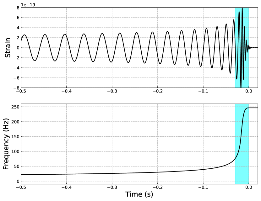
Figure 1: Evolution of the amplitude (upper panel) and frequency (lower panel) of the GWs produced by a GW150914-like BBH. In the calculation, the two BH masses are chosen to be $m_{1}=40\,M_{\odot}$ and $m_{2}=30\,M_{\odot}$, and the distance is set to $d=400$ Mpc.

Now that we know what the signal is like after the parameters are specified, can we reverse the process and estimate the parameters based on the signal? In the canonical scenario, i.e., the BBH is isolated in a vacuum background and not moving relative to us, the answer is yes.

Take the inspiral phase for example (since the chirp signal can be computed analytically). We can derive from the signal at least two measurable quantities, the amplitude $h$ and the frequency $f$. From the evolution of the frequency, we can further derive the time derivative $\dot{f}$. These three observables, $h$, $f$, and $\dot{f}$, encode the mass and distance of the source.

Since both $f$ and $\dot{f}$ are functions of the masses of the two BHs, $m_{1}$ and $m_{2}$, and the semimajor axis of the orbit, $a$, we can combine them to eliminate the dependence on $a$. We will show that the result is a quantity characterizing the mass of the system. First, we follow the Keplerian approximation, normally acceptable for the inspiral phase, and derive the GW frequency using twice the orbital frequency,

$$f=\frac{1}{\pi}\left[\frac{G(m_{1}+m_{2})}{a^{3}}\right]^{1/2},$$ (1)

where $G$ is the gravitational constant. Here we have assumed a circular orbit for simplicity. Elliptical orbits will lead to additional harmonics of different frequencies. Because of the GW radiation, the semi-major axis $a$ decays as

$$\dot{a}_{\rm gw}:=-\frac{64}{5}\frac{G^{3}m_{1}m_{2}(m_{1}+m_{2})}{c^{5}a^{3}},$$ (2)

where $c$ is the speed of light (as is derived in peters64 ). Combining the previous two equations, we can derive

$$\dot{f}=\dot{f}_{\rm gw}=\frac{96G^{7/2}m_{1}m_{2}(m_{1}+m_{2})^{3/2}}{5\pi c^{5}a^{11/2}},$$ (3)

where $\dot{f}_{\rm gw}$ denotes the contribution from GW radiation only. Now we can eliminate the $a$ in Equation (3) using Equation (1). The result is

$$\frac{c^{3}}{G}\,\left(\frac{5f^{-11/3}\dot{f}}{96\pi^{8/3}}\right)^{3/5}=\frac{(m_{1}m_{2})^{3/5}}{(m_{1}+m_{2})^{1/5}}.$$ (4)

It is now clear that from the two observables $f$ and $\dot{f}$, one can derive a quantity of the dimension of mass,

$${\cal M}=\frac{(m_{1}m_{2})^{3/5}}{(m_{1}+m_{2})^{1/5}}.$$ (5)

This mass is knowns at the “chirp mass” because, as Equation (4) indicates, it determines how $f$ increases with time.

Besides the chirp mass, can we derive $m_{1}$ and $m_{2}$ separately? It is difficult if the orbit is nearly Keplerian. In this case, we have seen that $\dot{f}$ is determined only by $\cal{M}$. The mass ratio of the two BHs, $q:=m_{2}/m_{1}$ (assuming $m_{2}\leq m_{1}$), plays no role as long as $\cal{M}$ is fixed. However, as the binary shrinks to a size of about dozens of the gravitational radii, GR effect becomes significant and the orbit starts to deviate from Keplerian motion. In fact, the deviation is $q$-dependent. Therefore, we can use it to disentangle the masses of the two BHs.

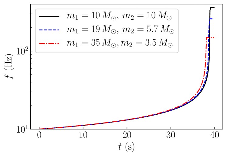
Figure 2: Chirp signals of three BBHs with the same chirp mass, ${\cal M}\simeq 8.7$, but different mass ratios, $q=1$, $1/3$, and $1/10$. The effect of different mass ratio starts to appear when $f$ exceeds about $20$ Hz.

To illustrate this idea, we show in Figure 2 the chirp signals of three BBHs with the same chirp mass but different mass ratios. To include the GR effects, the waveforms are computed to the 3.5 post-Newtonian order sathyaprakash09 . Since the chirp masses are the same, the three signals are almost identical when $f\lesssim 15$ Hz. At the later evolutionary stage when $f\gtrsim 20$ Hz, we start to see a divergence. The most prominent difference is the final frequency. We can see that higher frequency is correlated with larger mass ratio ($q$ approaches $1$). This is because as $q$ increases, the mass of the primary BH ($m_{1}$) decreases, so that the inner most circular orbit (ISCO) is smaller, and the corresponding frequency is higher.

This general result suggests that one has to detect the final merger to be able to measure the mass ratio of a BBH. This is the reason that LIGO and Virgo, by detecting GWs in the $10-10^{2}$ band, are capable of estimating the masses of individual BHs in binaries. The Laser Interferometer Space Antenna (LISA, see amaro17 ), on the other hand, can detect only the early inspiral phase of (stellar-mass) BBHs because LISA is tuned to be sensitive to milli-Hz (mHz) GWs. As a result, it is generally more difficult for LISA to measure the individual masses of (stellar-mass) BHs. It is worth noting that LISA is capable of measuring the masses of intermediate-massive and supermassive BHs between $10^{3}$ and $10^{10}\,M_{\odot}$, because their final mergers produce mHz GWs.

How about measuring the distance? So far, we have not yet used the third observable $h$. In principle, it is inversely proportional to the distance because larger distance should lead to smaller GW amplitude. In fact, in the Keplerian approximation the distance $d$ depends on $h$ as

$$d=\frac{4G}{c^{2}}\frac{{\cal M}}{h}\left(\frac{G}{c^{3}}\pi\,f\,{\cal M}\right)^{2/3}.$$ (6)

Here we have omitted the uncertainty induced by the inclination of the binary orbit because in principle it can be eliminated by measuring the GW polarizations. The important point is that all the quantities on the right-hand-side of the last equation can be derived from the three observables $f$, $\dot{f}$, and $h$. This completes the theory of measuring the mass and distance of a BBH using the chirp signal.

4 Mass-redshift degeneracy

In the last section, we have assumed a flat, Minkowski space. Because of this assumption, the signal detected is identical to the signal emitted from the source. However, the expansion of the universe will complicate this relationship. The cosmological expansion effectively stretches the signal. Consequently, the detected GWs will appear redshifted. Figure 3 illustrates this effect. From such a distorted signal, can we still retrieve the correct mass and distance of the source?

As a result of the cosmological redshift, the apparent frequency $f_{o}$ will be lower than the intrinsic frequency $f$ measured in the rest frame of the source. The difference can be calculated with

$$f_{o}=f(1+z_{\rm cos})^{-1},$$ (7)

where $z_{\rm cos}$ denotes the cosmological redshift. Moreover, to the observer the chirp rate appears to be

$$\dot{f}_{o}=\dot{f}_{\rm gw}(1+z_{\rm cos})^{-2},$$ (8)

where the additional factor of $(1+z_{\rm cos})^{-1}$ is due to time dilation. The students can verify the above equation by noticing that $\dot{f}_{o}=df_{o}/dt_{o}$ and $dt/dt_{o}=(1+z_{\rm cos})^{-1}$. If we wish to derive a chirp mass from the observed, redshifted signal, we can only get

$${\cal M}_{o}=\frac{c^{3}}{G}\,\left(\frac{5f_{o}^{-11/3}\dot{f_{o}}}{96\pi^{8/3}}\right)^{3/5}={\cal M}(1+z_{\rm cos}).$$ (9)

This new mass is greater than the intrinsic chirp mass by a redshift factor $1+z_{\rm cos}$. For this reason, it is called the “redshifted chirp mass”.

Now we have a problem. The mass appears greater than the intrinsic one. More seriously, without knowing the cosmological redshift of the source, we would not know the real mass. This famous problem in GW astronomy is called “the mass-redshift degeneracy”. Given such a problem, should we trust the BH masses derived from GWs, especially when the detected BHs seem a bit overweight?

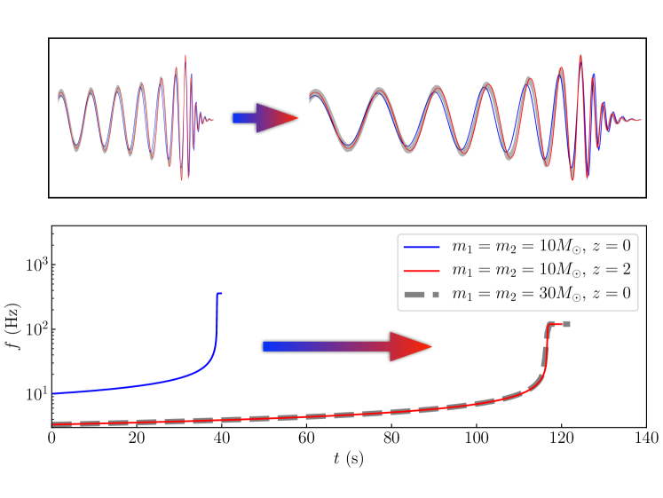
Figure 3: Effects of redshift on GW signals. Upper panel: Redshift stretches a waveform. Lower panel: An illustration of the problem of mass-redshift degeneracy. The intrinsic chirp signal of a $10-10\,M_{\odot}$ binary (blue solid curve) gets redshifted if the binary is placed at a redshift of $z=2$ (red solid curve). The redshifted signal is identical to that of a more massive, $30-30\,M_{\odot}$ binary residing at $z=0$ (grey dashed curve).

There are two possibilities of breaking this degeneracy. One possibility is to first measure the distance using GWs and then infer the redshift based on a chosen cosmological model. But what kind of distance is measurable from GWs in an expanding universe? Let us take the $\Lambda$CDM cosmology for example ($h=0.7$, $\Omega_{M}=0.29$, and $\Omega_{\Lambda}=0.71$). In this cosmology, the GW amplitude an observer detects is related to the transverse comoving distance $d_{C}$ as

$$h_{o}=\frac{4G}{c^{2}}\frac{{\cal M}}{d_{C}}\left(\frac{G}{c^{3}}\pi\,f\,{\cal M}\right)^{2/3},$$ (10)

where $f$ and $\cal{M}$ refer to the intrinsic, non-redshifted quantities. Using this apparent GW amplitude, we can only infer a distance of

$$d_{o}=\frac{4G}{c^{2}}\frac{{\cal M}_{o}}{h_{o}}\left(\frac{G}{c^{3}}\pi\,f_{o}\,{\cal M}_{o}\right)^{2/3}.$$ (11)

Substituting the observed quantities on the right-hand-side (those with the subscript $o$) using Equations (7), (9), and (10), one will find that

$$d_{o}=d_{C}(1+z_{\rm cos})=d_{L},$$ (12)

where $d_{L}$ is the luminosity distance. Therefore, what we derive from a chirp signal is in fact the luminosity distance. From the luminosity distance, we can calculate the corresponding redshift based on the chosen cosmological model. Finally, with this redshift, we can break the mass-redshift degeneracy.

To illustrate this idea, we show in Figure 4 the effect of cosmological expansion on the apparent chirp mass and distance of the first GW event GW150914. In the $\Lambda$CDM cosmology we have chosen, the apparent distance $d_{o}$ is identical to the luminosity distance, which corresponds to a redshift of $z_{\rm cos}\simeq 0.09$. Therefore, we can infer that the intrinsic chirp mass ${\cal M}$ is smaller than the apparent one, ${\cal M}_{o}$, by only a factor of about $1.1$. For this reason, it is believed that the BHs in GW150914 are intrinsically massive.

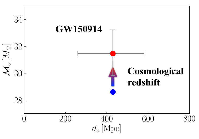
Figure 4: The effect of cosmological redshift on the apparent mass and distance of GW150914. The blue dot marks the location of the real chirp mass and (luminosity) distance of the source. The red dot shows the redshifted chirp mass and apparent distance, measureable from GW signal.

Another possibility is that an electromagnetic counterpart associated with a GW event is also detected. Then the redshift can be measured independently, e.g., from the spectrum. Detecting the electromagnetic counterpart will greatly enhance the scientific payback of GW observations. With the redshift $z_{\rm cos}$ derived from the counterpart and the luminosity distance $d_{L}$ from the GW signal, one can measure the Hubble constant and, in turn, constrain cosmological models. Unfortunately, detecting electromagnetic counterparts is challenging with the current telescopes. Moreover, some GW events, such as BBHs merging in a vacuum background, are not expected to produce strong electromagnetic radiation.

5 Effects of astrophysical environments

The standard model of a BBH merger does not take into account the motion of the binary relative to the observer. Neither does it include other astrophysical objects, or matter around the BHs or along the path of the propagation of GWs. Now we will add these new ingredients into our model and study the potential impact on our measurement of the physical parameters of the source.

5.1 Strong gravitational lensing

Strong gravitational lensing by foreground galaxies or galaxy clusters has been observed for transient light sources, such as supernovae and gamma-ray bursts. It is reasonable to speculate that some LIGO/Virgo events may also be lensed.

The effect of strong lensing is to magnify the amplitude of GWs. The significance can be characterized by the magnification factor ${\cal A}$, such that

$$h_{o}={\cal A}\left(\frac{4G}{c^{2}}\frac{{\cal M}}{d_{C}}\right)\left(\frac{G}{c^{3}}\pi\,f\,{\cal M}\right)^{2/3}.$$ (13)

According to Equation (11), the distance of a lensed GW sources will appear to be

$$d_{o}=d_{L}/\cal{A},$$ (14)

which is smaller than the real luminosity distance. The apparent mass, which one would derive from the GW signal, remains

$${\cal M}_{o}={\cal M}(1+z_{\rm cos}).$$ (15)

Figure 5 illustrates this effect using GW150914 as an example. It shows that a low-mass BBH residing at a high redshift, if getting gravitationally lensed, would appear as a high-mass binary residing at a relatively low redshift (as has been pointed out in broadhurst18 ; smith18 ). Now we cannot use the apparent distance $d_{o}$ to break the mass-redshift degeneracy, because it does not reflect the real luminosity distance of the source.

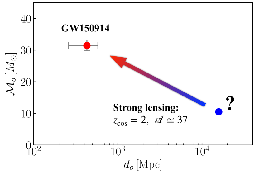
Figure 5: The lensing model of GW150914. For illustrative purposes, the source (blue dot) is placed at a cosmological redshift of $z_{\rm cos}=2$, corresponding to a luminosity distance of $16$ Gpc in the $\Lambda$CDM cosmology. After lensing, the mass and distance appear to coincide with those of GW150914 (red dot). The corresponding magnification factor is ${\cal A}\simeq 37$.

Could strong lensing explain all the massive BBHs detected by LIGO and Virgo? It is difficult because from the statistical point of view, lensing events should be uncommon. Moreover, as is indicated by the direction of the arrow in Figure 5, the lensing effect tends to produce an anti-correlation between the observed quantities $d_{o}$ and ${\cal M}_{o}$ broadhurst18 . The current observations do not favor such a relation abbott19GWTC . However, as the number of LIGO/Virgo BBHs increase and the detection horizon expands, the possibility of catching a lensed event increases as well. Therefore, watch out for massive BBHs at relatively low redshift!

5.2 The effect of motion

Almost all astrophysical objects are moving relative to us. The general effect of motion is to induce a Doppler shift to the frequency of a wave signal. This shift can be characterized by the relativistic Doppler factor,

$$1+z_{\rm dop}=\gamma(1+\vec{v}\cdot\vec{n}/c),$$ (16)

where $\vec{v}$ is the velocity of the source, $\vec{n}$ is a unit vector coinciding with the line-of-sight, and $\gamma=1/\sqrt{1-(v/c)^{2}}$ is the Lorentz factor.

Using this factor and taking the cosmological redshift into account, the apparent frequency can be written as

$$f_{o}=f(1+z_{\rm cos})^{-1}(1+z_{\rm dop})^{-1},$$ (17)

and the chirp rate changes to

$$\dot{f}_{o}=\dot{f}_{\rm gw}(1+z_{\rm cos})^{-2}(1+z_{\rm dop})^{-2}.$$ (18)

Applying Equation (9) again, we find that the apparent chirp mass is

$${\cal M}_{o}={\cal M}(1+z_{\rm cos})(1+z_{\rm dop}).$$ (19)

As for the distance, we notice that motion does not significantly affect the amplitude of GWs torres-orjuela19 . Therefore, we can follow Equation (10) to calculate $h_{o}$, and further derive that

$$d_{o}=d(1+z_{\rm cos})(1+z_{\rm dop}).$$ (20)

The last two equations suggest that Doppler shift can also affect the measurement of the mass and distance of BBH. It introduces a systematic error if not appropriately accounted for in GW data analysis. In particular, when the relative velocity and the line-of-sight are aligned, i.e., $\vec{v}\cdot\vec{n}>0$, the Doppler effect would make the mass and distance appear even greater than their intrinsic values.

We note one difference between the Doppler effect and the cosmological redshift. While cosmological redshift always makes the mass and distance appear bigger, Doppler effect could make them appear smaller as well. This happens when the source is moving towards the observer, i.e., when $\vec{v}\cdot\vec{n}<0$. In this case, the Doppler factor, as well as the effective redshift factor $1+z_{\rm dop}$, becomes smaller than $1$.

How large could the factor $1+z_{\rm dop}$ be? In the conventional scenario, BBHs form either in isolated binaries in galaxy bulges and disks, or in star clusters ligo16astro . In our Milky Way, isolated binaries and star clusters are moving at a typical velocity of $200\,{\rm km\,s^{-1}}$ relative to the earth. Therefore, their Doppler effect can be neglected. For the BBHs in external galaxies, their velocities relative to the Milky Way could be much greater. For example, in the most massive galaxy clusters, the velocities of the galaxy members can reach thousands of ${\rm km\,s^{-1}}$. Even this velocity is much smaller than the speed of light. For these reasons, Doppler effect is neglected in the standard procedure of GW data analysis.

However, the conventional picture of BBH formation is incomplete. Recent studies suggest that in galaxy centers, especially where there are SMBHs, the merger rate of BBHs can be enhanced. The reasons are multifold chen19 . (i) Close to a SMBH, the escape velocity is large. This is a place where newly formed compact objects are likely to stay. (ii) SMBHs are normally surrounded by a cluster of stars, known as the “nuclear star cluster”. Due to a net loss of energy during the gravitational interaction with other stars, massive objects such as BHs and neutron stars will gradually segregate towards the center of a nuclear star cluster. This “mass segregation effect” increases even higher the concentration of compact objects near SMBHs. Such a condition is favorable to the formation of BBHs. (iii) The tidal force exerted by SMBHs could excite the eccentricities of the nearby BBHs through the so-called “Lidov-Kozai” mechanism. A higher eccentricity normally results in a stronger GW radiation, and hence leads to a faster merger. (iv) If a SMBH is surrounded by gas, as would be the case in an active galactic nucleus (AGN) due to the presence of a gaseous accretion disk, interaction with the gas could also dissipate the internal energy of a BBH and lead to its faster merger.

Therefore, it is possible that a BBH may merge in the vicinity of a SMBH. If such a merger happens, the binary is likely to obtain a large velocity due to the orbital motion around the SMBH. For a BBH detected by LIGO/Virgo, the velocity is almost constant because the event lasts normally less than a second but the orbital period around the SMBH is orders of magnitude longer. The tidal force of the SMBH does not significantly affect the shrinkage of the binary because GW radiation predominates at this stage. Under these conditions, the theory developed in this section applies.

It is clear that the effect is more significant if the merger happens closer to the SMBH. We can use the velocities at the last stable orbits to estimate the order of magnitude of the maximum effect. If the binary is on a circular orbit around the SMBH, as we would expect for the BBHs in AGN accretion disks, the largest velocity appears at the ISCO. For non-spinning Schwarzschild BHs, the orbit is at a radius of $R=6GM/c^{2}$, where $M$ is the mass of the SMBH. In this case, the velocity is approximately $c/\sqrt{6}\simeq 0.408c$. The corresponding Doppler factor is $1+z_{\rm dop}\simeq 1.54$. On the other hand, if the orbit of the BBH is nearly parabolic, a more likely configuration if the binary forms far away and later gets captured by the SMBH, the last orbit is the innermost bound orbit (IBO). In this case, the pericenter is at $4GM/c^{2}$. The corresponding velocity is $c/\sqrt{2}=0.707c$ and the Doppler factor becomes $1+z_{\rm dop}\simeq 2.41$. Of course, even higher values are possible if the distance is smaller, but such events are rarer. The values derived above suggest that the Doppler effect could significantly affect our measurement of the mass and distance of a GW source, if the source is close to a SMBH. The event rate, therefore, deserves careful calculation.

5.3 Deep gravitational potential

Close to a SMBH, gravitational redshift is also significant. This additional redshift would further distort a GW signal and make the measurement of the physical parameters even more biased.

Suppose the gravitational redshift is $z_{\rm gra}$, the observed GW frequency would be lowered relative to the emitted one by a factor of $1+z_{\rm gra}$. Similar to the cosmological redshift and the Doppler effect, the chirp rate would be reduced by a factor of $(1+z_{\rm gra})^{2}$ due to time dilation. Using these relations, it is straightforward to show that the chirp mass appears to be

$${\cal M}_{o}={\cal M}(1+z_{\rm cos})(1+z_{\rm dop})(1+z_{\rm gra})$$ (21)

to an observer. To derive the apparent distance, we notice that the GW amplitude is not significantly affected by the gravitational redshift as long as the merger does not happen extremely close to the event horizon (see chen19 for a more quantitative description). As a result, Equation (10) remains a good approximation, from which we can derive that

$$d_{o}=d_{C}(1+z_{\rm cos})(1+z_{\rm dop})(1+z_{\rm gra}).$$ (22)

We can see that the apparent mass and distance of a BBH are determined by three types of redshift. Nevertheless, LIGO/Virgo only considered the cosmological redshift in their analysis. Such a treatment is not suitable for the BBHs forming in the vicinity of SMBHs.

We can again evaluate how extreme the value of $(1+z_{\rm dop})(1+z_{\rm gra})$ could be by investigating the last stable orbits. Assuming a non-spinning SMBH, we can calculate the gravitational redshift by

$$1+z_{\rm gra}=(1-R_{S}/R)^{-1/2},$$ (23)

where $R_{S}=2GM/c^{2}$ is the Schwarzschild radius. Using this equation, we find that for ISCO, the value of $(1+z_{\rm dop})(1+z_{\rm gra})$ is approximately $1.89$, while for IBO, it is about $3.41$.

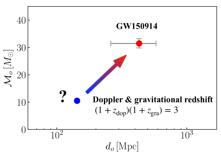
Figure 6: The Doppler-plus-gravitational-redshift model for GW150914. The location of the intrinsic chirp mass and luminosity distance is marked by the blue dot. The location of the apparent mass and distance is shown by the red dot. In the plot, a total redshift factor of $(1+z_{\rm dop})(1+z_{\rm gra})=3$ is assumed, which corresponds to a place close to the pericenter of the IBO around a Schwarzschild SMBH.

Interestingly, the values of these redshift factors coincide with the difference between the BH masses in GW150914 ($\sim 30\,M_{\odot}$) and those in X-ray binaries ($\sim 10\,M_{\odot}$). Could the Doppler$+$gravitational redshift explain the high-mass BHs detected by LIGO and Virgo (see Figure 6)? The key to answer this question is, again, the event rate. More works along this line of research are deserved.

5.4 Peculiar acceleration

For a binary orbiting a SMBH or any other tertiary object, the velocity of the center-of-mass of the binary in principle is not constant. This acceleration may not be a problem for LIGO/Virgo binaries because the event lasts only a fraction of a second, too short compared to the orbital period of the tertiary to cause any noticeable changes of the velocity. However, for LISA BBHs, the acceleration is no longer negligible. This is because LISA sources could dwell in the band for years. During this period, the velocity of the binaries may change significantly. This in turn changes the Doppler redshift meiron16 ; inayoshi17 .

Let us study the effect of this peculiar acceleration (different from the acceleration of the cosmological expansion) on our measurement of the mass and distance of binary compact objects. Starting from Equation (17) and neglecting the cosmological redshift for the time being, we can rewrite the relationship between the apparent frequency and the center-of-mass velocity of the binary as

$$f_{o}=f\frac{\sqrt{1-\beta^{2}}}{1+\vec{v}\cdot\vec{n}/c},$$ (24)

where $\beta=v/c$ and $f$ remains twice the orbital frequency. Differentiate it relative to the observer’s time, $t_{o}$, we get

$$\dot{f}_{o} =\frac{df_{o}}{dt_{o}}=\frac{dt}{dt_{o}}\frac{df_{o}}{dt}=\frac{1}{1+z_{\rm dop}}\left[\frac{\dot{f}_{\rm gw}}{1+z_{\rm dop}}+f\frac{d}{dt}\left(\frac{\sqrt{1-\beta^{2}}}{1+\vec{v}\cdot\vec{n}/c}\right)\right]$$ (25)

$$=\frac{\dot{f}_{\rm gw}}{(1+z_{\rm dop})^{2}}+f_{o}\frac{d}{dt}\left(\frac{\sqrt{1-\beta^{2}}}{1+\vec{v}\cdot\vec{n}/c}\right).$$ (26)

If we compare the last equation with Equation (18) and notice that $z_{\rm cos}=0$ for now, we will see that the second term on the right-hand-side of the last equation is caused by the variation of $\vec{v}$. This term could be either positive or negative, depending on the orbital dynamics. Therefore, the apparent chirp mass, which should be calculated from $f_{o}$ and $\dot{f}_{o}$, could also be bigger or smaller than the real value, and so does the apparent distance. To further quantify this effect, we define $\Gamma_{\rm acc}$ to be the ratio between the second and the first term in Equation (26). This treatment allows us to write ${\cal M}_{o}$ and $d_{o}$ in the following compact forms,

$${\cal M}_{o}={\cal M}(1+z_{\rm dop})(1+\Gamma_{\rm acc})^{3/5},$$ (27)

and

$$d_{o}=d(1+z_{\rm dop})(1+\Gamma_{\rm acc}).$$ (28)

In particular, Equation (27) indicates that mass is degenerate with not only redshift but also acceleration. This is a new type of degeneracy in GW astronomy. Notice that $\Gamma_{\rm acc}$ could be negative so that $1+\Gamma_{\rm acc}$ may be smaller than $0$. In this case, we see an inverse chirp, i.e., the GW frequency decreases with time. Such a signal immediately indicates a non-standard condition for the binary. These events could be singled out in data analysis without causing further confusion. Therefore, in the following we focus on the case in which $1+\Gamma_{\rm acc}>0$.

For those binaries in triple systems, when will $\Gamma_{\rm acc}$ significantly exceed unity? Since $\dot{f}_{\rm gw}\propto f^{11/3}$, the value of $\Gamma_{\rm acc}$ is higher for lower $f$. This is another reason that we focus on LISA binaries in this section. To derive a value for $\Gamma_{\rm acc}$, we must specify the parameters of the tertiary. For simplicity, we assume circular orbits for the tertiary. In this case, the second term on the right-hand-side of Equation (26) is of the order of $Gm_{3}f_{o}/(r^{2}c)$, where $m_{3}$ is the mass of the tertiary and $r$ is the distance between the tertiary and the center-of-mass of the binary. Here we have omitted the term $\sqrt{1-\beta^{2}}$ because we only consider the case in which the center-of-mass velocity is much smaller than the speed of light. This consideration is acceptable for LISA binaries because they cannot reside at several Schwarzschild radii of a SMBH. Otherwise, the binaries would be tidally disrupted given their large semimajor axes. Using this approximation for the acceleration, we find that

$$\Gamma_{\rm acc}\simeq 4.4\left(\frac{f}{2\,{\rm mHz}}\right)^{-8/3}\left(\frac{{\cal M}}{0.3\,M_{\odot}}\right)^{-5/3}\left(\frac{m_{3}}{1\,M_{\odot}}\right)\left(\frac{r}{30\,{\rm AU}}\right)^{-2}.$$ (29)

This result suggests that the acceleration affects more seriously the low-mass binaries (small ${\cal M}$) in the LISA band. Let us take DWDs for example since they are the most numerous binaries in band amaro17 . If we assume ${\cal M}=0.3\,M_{\odot}$ and set $f=2$ mHz, the most sensitive band of LISA, we find that $\Gamma_{\rm acc}=4.4$ for a tertiary of $m_{3}=1\,M_{\odot}$ and $r=20$ AU. Corresponding, the chirp mass appears bigger, due to the term $(1+\Gamma_{\rm acc})^{3/5}$, by a factor of $2.8$. The distance, on the other hand, appears bigger by a factor of about $5.4$. In this case, a DWD inside the Milky Way would appear in a nearby galaxy! If, on the other hand, we reverse the orbital velocity of the tertiary and increase the chirp mass to $0.8\,M_{\odot}$, we will get $\Gamma_{\rm acc}=-0.86$. In this case, the DWD will appear lighter by a factor of $3.2$ and closer by a factor of $7.0$! Similar cases could potentially impede our understanding of the formation and distribution of DWDs in the Milky Way.

If the tertiary is a SMBH, as would be the case for those DWDs forming in the Galactic Center, $\Gamma_{\rm acc}$ would be even greater. For example, if we assume $m_{3}=4\times 10^{6}\,M_{\odot}$ and $r=0.1$ pc, a DWD with ${\cal M}=0.3\,M_{\odot}$ and $f=2$ mHz will have $\Gamma_{\rm acc}=38$. The apparent chirp mass will increase to ${\cal M}_{o}\simeq 2.7\,M_{\odot}$. Now the white dwarfs will masquerade as neutron stars or BHs!

So far, the estimation of the chirp mass is based on only two observables, $f$ and $\dot{f}$. One may wonder that given the long observational period of LISA ($\sim 5$ years), could we derive also $\ddot{f}$ from the waveform? This is an important question because if we could measure $\ddot{f}$, maybe we could use it to break the degeneracy between mass and acceleration. In fact, for BBHs, more advanced data analysis does show that it is possible tamanini19 .

For DWDs, however, it is more difficult because the value of $\ddot{f}$ induced by either GW radiation or peculiar acceleration is small. As Figure (7) shows, such a chirp signal is featureless. The evolution of $f_{o}$ is effectively a straight line. Since we use the slope of the straight line to infer the chirp mass, and small BBHs with large acceleration lead to the same slopes as those big BBHs without acceleration, it is difficult to distinguish these two scenarios robson18 .

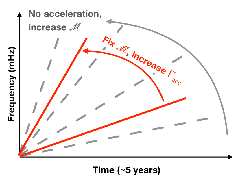
Figure 7: Illustration of the degeneracy between mass and acceleration. The evolution of the apparent frequency is effectively a straight line if the chirp mass of the source is intrinsically small, such as in the case of DWDs. The gray dashed lines show the dependence of the chirp signal on the chirp mass of the system. The red lines show the dependence on the acceleration. It is clear that the effect of increasing the acceleration is identical to the effect of increasing the chirp mass.

5.5 The effect of gas

Gas is another important factor for the formation and evolution of BBHs. For example, in the model of binary-star evolution, there is a phase when both binary members are immersed in a common gaseous envelope. This phase is considered to be essential to the formation of close binaries. Moreover, as has been mentioned before, AGN accretion disk is also a breeding ground for BBHs. In general, gas will change the orbital dynamics of a BBH, and in this way affect the GW signal. Without knowing of such an effect, would a GW observer retrieve correctly the physical parameters of a BBH?

We now know that to address this question, we need to investigate the effect of gas on $f$ and $\dot{f}$, and use them to derive the apparent chirp mass and distance. In fact, gas does not significantly affect $f$ because in the astrophysical scenarios mentioned above, the total mass of the gas is negligible relative to the total mass of the BHs. The effect is more prominent for $\dot{f}$. Depending on the thermal dynamical properties and the distribution, gas could either accelerate or decelerate the binary shrinkage, and hence increase or decrease $\dot{f}$ relative to $\dot{f}_{\rm gw}$. For example, hydrodynamical friction makes the binary orbit shrink faster but tidal torque and accretion could work in the opposite direction (see a brief discussion in chen20gas ).

To keep the following analysis general, we can characterize the gas effect by rewriting the apparent chirp rate as

$$\dot{f}_{o}=\dot{f}_{\rm gw}+\dot{f}_{\rm gas}=\dot{f}_{\rm gw}(1+\Gamma_{\rm gas}),$$ (30)

where $\dot{f}_{\rm gas}$ is the chirp rate due to gas dynamics and $\Gamma_{\rm gas}:=\dot{f}_{\rm gas}/\dot{f}_{\rm gw}$. The redshift effects are neglected here for simplicity. Similar to the analysis of peculiar acceleration, we can derive that

$${\cal M}_{o} ={\cal M}(1+\Gamma_{\rm gas})^{3/5},$$ (31)

$$d_{o} =d(1+\Gamma_{\rm gas}).$$ (32)

Since $\Gamma_{\rm gas}$ can be either positive or negative, the apparent mass and distance could be bigger or smaller than their intrinsic values. Figure 8 shows that the effect of increasing the efficiency of gas-dynamics (increasing $\Gamma_{\rm gas}$) is identical to the effect of increasing the chirp mass.

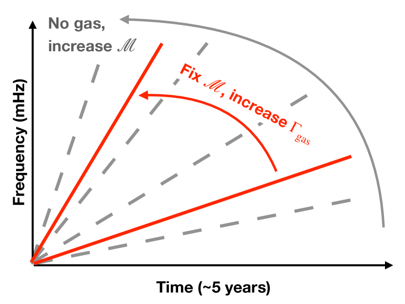
Figure 8: Same as Figure 7 but showing the effect of gas on the slope of the chirp signal.

Like the effect of peculiar acceleration, gas is more important for those binaries in the mHz. In this band, $\dot{f}_{\rm gw}$ is small so that the gas-induced $\dot{f}_{\rm gas}$ could be relatively large. Recent models show that in AGN accretion disks and common envelopes, $\Gamma_{\rm gas}$ could be much greater than $1$ chen19gas ; caputo20 ; chen20gas . Therefore, in these environments BBHs, as well DNSs and DWDs, could appear more massive than they really are.

6 Summary

In this chapter, we have seen that astrophysical factors could affect the measurement of the masses of GW sources. In particular, strong gravitational lensing, the Doppler and gravitational redshift around a SMBH, the peculiar acceleration induced by a tertiary star or SMBH, and gas dynamics could all increase the apparent chirp mass of a binary. In suitable conditions, the Doppler blueshift in the vicinity of a SMBH, the peculiar acceleration, and gas dynamics could also work in the opposite way, reducing the apparent mass.

These results have important implications for the peculiar compact objects appearing in the bands of LIGO/Virgo and the future LISA. Such peculiar objects include compact objects in the lower mass gap (between $3$ and $5\,M_{\odot}$) and BHs heavier than $20\,M_{\odot}$. They had never been detected in the past, before the GW era. Therefore, their nature deserves a thorough scrutiny.

Table 1: Alternatives models for the peculiar objects appearing in the LIGO/Virgo/LISA band.

Detector	Peculiar Objects	Imposters	Models	Notes
LIGO/Virgo	$\gtrsim 20\,M_{\odot}$	BBH $m_{1},\,m_{2}<20\,M_{\odot}$	1, 2, 4	i
		BNS	–	ii
		DWD	–	iii
	$(3,\,5)\,M_{\odot}$	BBH $m_{1},\,m_{2}\geq 5\,M_{\odot}$	3	iv
		BNS	2, 4	v
		DWD	–	vi
LISA	$\gtrsim 20\,M_{\odot}$	BBH $m_{1},\,m_{2}<20\,M_{\odot}$	6	vii
		BNS	6	viii
		DWD	6	ix
	$(3,\,5)\,M_{\odot}$	BBH $m_{1},\,m_{2}\geq 5\,M_{\odot}$	5, 6	x
		BNS	5, 6	xi
		DWD	5, 6	xii

1. Gravitational lensing; 2. Doppler redshift (SMBH); 3. Doppler blueshift (SMBH); 4. Gravitational redshift (SMBH); 5. Peculiar acceleration; 6. Gas dynamics.

Now we can revisit the question raised at the beginning of this chapter. Once LIGO/Virgo or LISA detect a peculiar object, could we readily accept the apparent mass as the real one, or what are the other possibilities? Table 6 summarizes the alternative possibilities. The following is a brief discussion of each case. Interested readers could refer to the previous sections for more detailed explanations.

1. In the LIGO/Virgo band ($10-10^{2}$ Hz), the BHs with an apparent mass higher than $20\,M_{\odot}$ could be mimicked by the BHs less massive than $20\,M_{\odot}$, due to strong lensing, or the Doppler and gravitational redshift around SMBHs. For the BBHs in this band, peculiar acceleration and gas dynamics are too weak relative to GW radiation to cause such an strong effect.

2. BNSs are unlikely imposters of the massive BBHs with $m_{1},\,m_{2}>20\,M_{\odot}$ in the LIGO/Virgo band. In the scenarios of strong lensing, Doppler redshift, and gravitational redshift, the BNSs should have a redshift of $z\gtrsim 10$ to meet the requirement. The corresponding magnification factor (${\cal A}$) would be too extreme, and the distance to SMBH too small. Such events are rare. Peculiar acceleration and gas dynamics are unlikely to take effect either. Because GW radiation would predominate the evolution of $\dot{f}_{o}$ as soon as the BNSs enter the LIGO/Virgo band.

3. DWDs cannot masquerade as massive BBHs in the LIGO/Virgo band either. Because of the large sizes of white dwarfs, the coalescence happens at a frequency of about $0.1$ Hz. Therefore, DWDs do not enter the LIGO/Virgo band.

4. The Doppler blueshift could also make an ordinary BH slightly more massive than $5\,M_{\odot}$ appear in the lower mass gap in LIGO/Virgo observations. For example, a BBH at the ISCO of a Schwarzschild SMBH could be blueshifted. Combined with the gravitational redshift, the apparent mass could be a factor of $(1+z_{\rm dop})(1+z_{\rm gra})\simeq 0.79$ of the real mass. For the IBO, the effect is more significant, and the fact could reduce to $0.58$. Around Kerr SMBHs, the factor could be even smaller. Peculiar acceleration and gas dynamics could hardly induce such an effect because, as is mentioned in (i), they are too weak compared to GW radiation.

5. BNSs merging in the vicinity of a SMBH could also appear in the lower-mass-gap in LIGO/Virgo observations, because of the Doppler and gravitational redshift. Strong lensing, on the other hand, is unlikely to cause such an effect, because BNSs have to be relatively nearby to be detected by LIGO/Virgo. Therefore, the probability of being lensed is low. For the same reason given in (ii), peculiar acceleration and gas dynamics are unlikely to move BNSs into the lower mass gap either.

6. Same as (iii).

7. For LISA, the GW frequency is low. The corresponding BBHs are at an early evolutionary stage and the GW power is relatively weak. In this case, gas dynamics could compete with GW radiation and make less massive BH appear in the mass range of $\gtrsim 20\,M_{\odot}$, while the effect of peculiar acceleration is still too weak to significantly affect $\dot{f}_{o}$. Strong lensing is unlikely because LISA BBHs are at relatively small luminosity distances. Doppler and gravitational redshift induced by a nearby SMBH is unlikely either, because LISA BBHs, due to their large semi-major axis, are likely to be tidally disrupted if they approach the Schwarzschild radius of a SMBH.

8. BNSs could masquerade as BBHs in the LISA band if there is gas around. The other models are unlikely to work here for the same reasons given in (vii).

9. The same as (vii) and (viii).

10. Since gas dynamics could also reduce $\dot{f}_{o}$, it could make the BHs more massive than $5\,M_{\odot}$ appear in the low mass gap in LISA observations. Peculiar acceleration could work in the same way, but only when the BHs are slightly more massive than $5\,M_{\odot}$ and the tertiary is a SMBH. Doppler blueshift around a SMBH could not induced such an effect because it would require BBHs to approach several Schwarzschild radii of the SMBH. LISA BBHs would be tidally disrupted at such a small distance.

11. BNSs could masquerade as lower-mass-gap objects in the LISA band due to the peculiar acceleration and gas-dynamical effects. Strong gravitational lensing has difficulty inducing such an effect because LISA BNSs are relatively close by. Doppler and gravitational redshift due to a nearby SMBH is unlikely to work here, because of the strong tidal force close to the SMBH.

12. The same as (xi), but the peculiar acceleration works only when the tertiary is a SMBH.

Estimating the corresponding event rate could help us evaluate the likelihood of the above models and, maybe, reject some of them abbott19population ; chen19 . But the estimation is subject to uncertainties because of our incomplete understanding of the astrophysical environments around GW sources. A more rigorous approach is to study the distortion of the wave front by those astrophysical factors and look for a detectable signature (e.g. hannuksela19 ; torres-orjuela19 ; torres-orjuela20 ). Both directions deserve further exploration.

References

- (1) B. P. Abbott, R. Abbott, T. D. Abbott, M. R. Abernathy, F. Acernese, K. Ackley, C. Adams, T. Adams, P. Addesso, R. X. Adhikari, and et al., “Observation of Gravitational Waves from a Binary Black Hole Merger,” Physical Review Letters, vol. 116, p. 061102, Feb. 2016.
- (2) LIGO Scientific Collaboration and Virgo Collaboration, “Binary Black Hole Population Properties Inferred from the First and Second Observing Runs of Advanced LIGO and Advanced Virgo,” Astrophysical Journal Letters, vol. 882, p. L24, Sept. 2019.
- (3) LIGO Scientific Collaboration and Virgo Collaboration, “GW190425: Observation of a compact binary coalescence with total mass 3.4 m ,” The Astrophysical Journal, vol. 892, p. L3, Mar 2020.
- (4) L. S. Collaboration and V. Collaboration, “Gw190521: A binary black hole merger with a total mass of ,” Physical Review Letters, vol. 125, p. 101102, Sep 2020.
- (5) M. C. Miller and D. P. Hamilton, “Four-Body Effects in Globular Cluster Black Hole Coalescence,” Astrophysical Journal, vol. 576, pp. 894–898, Sept. 2002.
- (6) F. Antonini and H. B. Perets, “Secular Evolution of Compact Binaries near Massive Black Holes: Gravitational Wave Sources and Other Exotica,” Astrophysical Journal, vol. 757, p. 27, Sept. 2012.
- (7) X. Chen, S. Li, and Z. Cao, “Mass-redshift degeneracy for the gravitational-wave sources in the vicinity of supermassive black holes,” Monthly Notices of the Royal Astronomical Society, vol. 485, pp. L141–L145, May 2019.
- (8) X. Chen, Z.-Y. Xuan, and P. Peng, “Fake Massive Black Holes in the Milli-Hertz Gravitational-wave Band,” Astrophysical Journal, vol. 896, p. 171, June 2020.
- (9) Y. Wang, A. Stebbins, and E. L. Turner, “Gravitational Lensing of Gravitational Waves from Merging Neutron Star Binaries,” Physical Review Letters, vol. 77, pp. 2875–2878, Sept. 1996.
- (10) T. T. Nakamura, “Gravitational Lensing of Gravitational Waves from Inspiraling Binaries by a Point Mass Lens,” Physical Review Letters, vol. 80, pp. 1138–1141, Feb. 1998.
- (11) R. Takahashi and T. Nakamura, “Wave Effects in the Gravitational Lensing of Gravitational Waves from Chirping Binaries,” Astrophysical Journal, vol. 595, pp. 1039–1051, Oct. 2003.
- (12) B. F. Schutz, “Determining the Hubble constant from gravitational wave observations,” Nature, vol. 323, p. 310, Sept. 1986.
- (13) P. C. Peters, “Gravitational Radiation and the Motion of Two Point Masses,” Physical Review, vol. 136, pp. 1224–1232, Nov. 1964.
- (14) B. S. Sathyaprakash and B. F. Schutz, “Physics, Astrophysics and Cosmology with Gravitational Waves,” Living Reviews in Relativity, vol. 12, p. 2, Dec. 2009.
- (15) P. Amaro-Seoane, H. Audley, S. Babak, J. Baker, E. Barausse, P. Bender, E. Berti, P. Binetruy, M. Born, and D. e. a. Bortoluzzi, “Laser Interferometer Space Antenna,” ArXiv e-prints, Feb. 2017.
- (16) T. Broadhurst, J. M. Diego, and I. Smoot, George, “Reinterpreting Low Frequency LIGO/Virgo Events as Magnified Stellar-Mass Black Holes at Cosmological Distances,” arXiv e-prints, p. arXiv:1802.05273, Feb. 2018.
- (17) G. P. Smith, M. Jauzac, J. Veitch, W. M. Farr, R. Massey, and J. Richard, “What if LIGO’s gravitational wave detections are strongly lensed by massive galaxy clusters?,” Monthly Notices of the Royal Astronomical Society, vol. 475, pp. 3823–3828, Apr. 2018.
- (18) LIGO Scientific Collaboration and Virgo Collaboration, “GWTC-1: A Gravitational-Wave Transient Catalog of Compact Binary Mergers Observed by LIGO and Virgo during the First and Second Observing Runs,” Physical Review X, vol. 9, p. 031040, July 2019.
- (19) A. Torres-Orjuela, X. Chen, Z. Cao, P. Amaro-Seoane, and P. Peng, “Detecting the beaming effect of gravitational waves,” Physical Review D, vol. 100, p. 063012, Sept. 2019.
- (20) B. P. Abbott, R. Abbott, T. D. Abbott, M. R. Abernathy, F. Acernese, K. Ackley, C. Adams, T. Adams, P. Addesso, R. X. Adhikari, and et al., “Astrophysical Implications of the Binary Black-hole Merger GW150914,” Astrophysical Journal Letters, vol. 818, p. L22, Feb. 2016.
- (21) Y. Meiron, B. Kocsis, and A. Loeb, “Detecting Triple Systems with Gravitational Wave Observations,” Astrophysical Journal, vol. 834, p. 200, Jan. 2017.
- (22) K. Inayoshi, N. Tamanini, C. Caprini, and Z. Haiman, “Probing stellar binary black hole formation in galactic nuclei via the imprint of their center of mass acceleration on their gravitational wave signal,” Physical Review D, vol. 96, p. 063014, Sept. 2017.
- (23) N. Tamanini, A. Klein, C. Bonvin, E. Barausse, and C. Caprini, “Peculiar acceleration of stellar-origin black hole binaries: Measurement and biases with LISA,” Physical Review D, vol. 101, p. 063002, Mar. 2020.
- (24) T. Robson, N. J. Cornish, N. Tamanini, and S. Toonen, “Detecting hierarchical stellar systems with LISA,” Physical Review D, vol. 98, p. 064012, Sept. 2018.
- (25) X. Chen and Z. Shen, “Retrieving the true masses of gravitational wave sources,” Proceedings, vol. 17, no. 1, p. 4, 2019.
- (26) A. Caputo, L. Sberna, A. Toubiana, S. Babak, E. Barausse, S. Marsat, and P. Pani, “Gravitational-wave Detection and Parameter Estimation for Accreting Black-hole Binaries and Their Electromagnetic Counterpart,” Astrophysical Journal, vol. 892, p. 90, Apr. 2020.
- (27) O. A. Hannuksela, K. Haris, K. K. Y. Ng, S. Kumar, A. K. Mehta, D. Keitel, T. G. F. Li, and P. Ajith, “Search for gravitational lensing signatures in LIGO-virgo binary black hole events,” The Astrophysical Journal, vol. 874, p. L2, mar 2019.
- (28) A. Torres-Orjuela, X. Chen, and P. Amaro-Seoane, “Phase shift of gravitational waves induced by aberration,” Physical Review D, vol. 101, p. 083028, Apr. 2020.