Fast convex optimization via inertial dynamics combining viscous and Hessian-driven damping with time rescaling

Abstract

In a Hilbert setting, we develop fast methods for convex unconstrained optimization. We rely on the asymptotic behavior of an inertial system combining geometric damping with temporal scaling. The convex function to minimize enters the dynamic via its gradient. The dynamic includes three coefficients varying with time, one is a viscous damping coefficient, the second is attached to the Hessian-driven damping, the third is a time scaling coefficient. We study the convergence rate of the values under general conditions involving the damping and the time scale coefficients. The obtained results are based on a new Lyapunov analysis and they encompass known results on the subject. We pay particular attention to the case of an asymptotically vanishing viscous damping, which is directly related to the accelerated gradient method of Nesterov. The Hessian-driven damping significantly reduces the oscillatory aspects. As a main result, we obtain an exponential rate of convergence of values without assuming the strong convexity of the objective function. The temporal discretization of these dynamics opens the gate to a large class of inertial optimization algorithms.

1 Introduction

Throughout the paper, $\mathcal{H}$ is a real Hilbert space with inner product $\langle\cdot,\cdot\rangle$ and induced norm $\|\cdot\|,$ and $f:\mathcal{H}\rightarrow{\mathbb{R}}$ is a convex and differentiable function. We aim at developping fast numerical methods for solving the optimization problem

$$({\mathcal{P}})\hskip 28.45274pt\min_{x\in\mathcal{H}}f(x).$$

We denote by $\hbox{argmin}_{\mathcal{H}}f$ the set of minimizers of the optimization problem $({\mathcal{P}})$, which is assumed to be non-empty. Our work is part of the active research stream that studies the close link between continuous dissipative dynamical systems and optimization algorithms. In general, the implicit temporal discretization of continuous gradient-based dynamics provides proximal algorithms that benefit from similar asymptotic convergence properties, see PS for a systematic study in the case of first-order evolution systems, and att8 ; att9 ; ACFR ; att6 ; ACR-Pafa-2019 ; Bot1 ; Bot2 ; Bot3 for some recent results concerning second-order evolution equations. The main object of our study is the second-order in time differential equation

$${\rm(IGS)}_{\gamma,\beta,b}\hskip 28.45274pt\ddot{x}(t)+\gamma(t)\dot{x}(t)+\beta(t)\nabla^{2}f(x(t))\dot{x}(t)+b(t)\nabla f(x(t))=0,$$

where the coefficients $\gamma,\beta:[t_{0},+\infty[\rightarrow{\mathbb{R}}_{+}$ take account of the viscous and Hessian-driven damping, respectively, and $b:{\mathbb{R}}_{+}\to{\mathbb{R}}_{+}$ is a time scale parameter. We take for granted the existence and uniqueness of the solution of the corresponding Cauchy problem with initial conditions $x(t_{0})=x_{0}\in{\mathcal{H}}$, $\dot{x}(t_{0})=v_{0}\in{\mathcal{H}}$. Assuming that $\nabla f$ is Lipschitz continuous on the bounded sets, and that the coefficients are continuously differentiable, the local existence follows from the nonautonomous version of the Cauchy-Lipschitz theorem, see (haraux, , Prop. 6.2.1). The global existence then follows from the energy estimates that will be established in the next section. Each of these damping and rescaling terms properly tuned, improves the rate of convergence of the associated dynamics and algorithms. An original aspect of our work is to combine them in the same dynamic. Let us recall some classical facts.

1.1 Damped inertial dynamics and optimization

The continuous-time perspective gives a mechanical intuition of the behavior of the trajectories, and a valuable tool to develop a Lyapunov analysis. A first important work in this perspective is the heavy ball with friction method of B. Polyak polyak

$${\rm(HBF)}\quad\ddot{x}(t)+\gamma\dot{x}(t)+\nabla f(x(t))=0.$$

It is a simplified model for a heavy ball (whose mass has been normalized to one) sliding on the graph of the function $f$ to be minimized, and which asymptotically stops under the action of viscous friction, see AGR for further details. In this model, the viscous friction parameter $\gamma$ is a fixed positive parameter. Due to too much friction (at least asymptotically) involved in this process, replacing the fixed viscous coefficient with a vanishing viscous coefficient (i.e.  which tends to zero as $t\to+\infty$) gives Nesterov’s famous accelerated gradient method nestro1 nestro2 . The other two basic ingredients that we will use, namely time rescaling, and Hessian-driven damping have a natural interpretation (cinematic and geometric, respectively) in this context. We will come back to these points later. Precisely, we seek to develop fast first-order methods based on the temporal discretization of damped inertial dynamics. By fast we mean that, for a general convex function $f$, and for each trajectory of the system, the convergence rate of the values $f(x(t))-\inf_{{\mathcal{H}}}f$ which is obtained is optimal (i.e.  is achieved of nearly achieved in the worst case). The importance of simple first-order methods, and in particular gradient-based and proximal algorithms, comes from the applicability of these algorithms to a wide range of large-scale problems arising from machine learning and/or engineering.

1.1.1 The viscous damping parameter $\gamma(t)$.

A significant number of recent studies have focused on the case $\gamma(t)=\frac{\alpha}{t}$, $\beta=0$ (without Hessian-driven damping), and $b=1$ (without time rescaling), that is

$${\rm(AVD)}_{\alpha}\hskip 28.45274pt\ddot{x}(t)+\frac{\alpha}{t}\dot{x}(t)+\nabla f(x(t))=0.$$

This dynamic involves an Asymptotically Vanishing Damping coefficient (hence the terminology), a key property to obtain fast convergence for a general convex function $f$. In boyd , Su, Boyd and Candès showed that for $\alpha=3$ the above system can be seen as a continuous version of the accelerated gradient method of Nesterov nestro1 ; nestro2 with $f(x(t))-\min_{\mathcal{H}}f=\mathcal{O}(\frac{1}{t^{2}})$ as $t\to+\infty$. The importance of the parameter $\alpha$ was put to the fore by Attouch, Chbani, Peypouquet and Redont redon and May may . They showed that, for $\alpha>3$, one can pass from capital $\mathcal{O}$ estimates to small $o$. Moreover, when $\alpha>3$, each trajectory converges weakly, and its limit belongs to $\operatorname{argmin}f$. Recent research considered the case of a general damping coefficient $\gamma(\cdot)$ (see cabot1 ; att2 ), thus providing a complete picture of the convergence rates for ${\rm(AVD)}_{\alpha}$: $f(x(t))-\min_{\mathcal{H}}f=\mathcal{O}(1/t^{2})$ when $\alpha\geq 3$, and $f(x(t))-\min_{\mathcal{H}}f=\mathcal{O}\left(1/t^{\frac{2\alpha}{3}}\right)$ when $\alpha\leq 3$, see att2 ; att1 and Apidopoulos, Aujol and Dossal AAD .

1.1.2 The Hessian-driven damping parameter $\beta(t)$.

The inertial system

$${\rm\mbox{(DIN)}}_{\gamma,\beta}\qquad\ddot{x}(t)+\gamma\dot{x}(t)+\beta\nabla^{2}f(x(t))\dot{x}(t)+\nabla f(x(t))=0,$$

was introduced by Alvarez, Attouch, Bolte, and Redont in AABR . In line with (HBF), it contains a fixed positive friction coefficient $\gamma$. As a main property, the introduction of the Hessian-driven damping makes it possible to neutralize the transversal oscillations likely to occur with (HBF), as observed in AABR . The need to take a geometric damping adapted to $f$ had already been observed by Alvarez Alvarez who considered the inertial system

$$\ddot{x}(t)+\mathcal{D}\dot{x}(t)+\nabla f(x(t))=0,$$

where $\mathcal{D}:{\mathcal{H}}\to{\mathcal{H}}$ is a linear positive definite anisotropic operator. But still this damping operator is fixed. For a general convex function, the Hessian-driven damping in $\mbox{\rm(DIN)}_{\gamma,\beta}$ performs a similar operation in a closed-loop adaptive way. (DIN) stands shortly for Dynamical Inertial Newton, and refers to the link with the Levenberg-Marquardt regularization of the continuous Newton method. Recent studies have been devoted to the study of the inertial dynamic

$$\ddot{x}(t)+\frac{\alpha}{t}\dot{x}(t)+\beta\nabla^{2}f(x(t))\dot{x}(t)+\nabla f(x(t))=0,$$

which combines asymptotic vanishing damping with Hessian-driven damping APR .

1.1.3 The time rescaling parameter b(t).

In the context of non-autonomous dissipative dynamic systems, reparameterization in time is a simple and universal means to accelerate the convergence of trajectories. This is where the coefficient $b(t)$ comes in as a factor of $\nabla f(x(t))$. In att6 ACR-Pafa-2019 , in the case of general coefficients $\gamma(\cdot)$ and $b(\cdot)$ without the Hessian damping, the authors made in-depth study. In the case $\gamma(t)=\frac{\alpha}{t}$, they proved that under appropriate conditions on $\alpha$ and $b(\cdot)$, $f(x(t))-\min_{\mathcal{H}}f=\mathcal{O}(\frac{1}{t^{2}b(t)})$. Hence a clear improvement of the convergence rate by taking $b(t)\to+\infty$ as $t\to+\infty$.

1.2 From damped inertial dynamics to proximal-gradient inertial algorithms

Let’s review some classical facts concerning the close link between continuous dissipative inertial dynamic systems and the corresponding algorithms obtained by temporal discretization. Let us insist on the fact that, when the temporal scaling $b(t)\to+\infty$ as $t\to+\infty$, the transposition of the results to the discrete case naturally leads to consider an implicit temporal discretization, i.e.  inertial proximal algorithms. The reason is that, since $b(t)$ is in front of the gradient, the application of the gradient descent lemma would require taking a step size that tends to zero. On the other hand, the corresponding proximal algorithms involve a proximal coefficient which tends to infinity (large step proximal algorithms).

1.2.1 The case without the Hessian-driven damping

The implicit discretization of ${\rm(IGS)}_{\gamma,0,b}$ gives the Inertial Proximal algorithm

$${\rm(IP)}_{\alpha_{k},\lambda_{k}}\hskip 28.45274pt\left\{\begin{array}[]{l}y_{k}=x_{k}+\alpha_{k}(x_{k}-x_{k-1})\vspace{2mm}\\ x_{k+1}=\hbox{prox}_{\lambda_{k}f}(y_{k})\end{array}\right.$$

where $\alpha_{k}$ is non-negative and $\lambda_{k}$ is positive. Recall that for any $\lambda>0$, the proximity operator $\hbox{prox}_{\lambda f}:{\mathcal{H}}\to{\mathcal{H}}$ is defined by the following formula: for every $x\in{\mathcal{H}}$

$$\hbox{prox}_{\lambda f}(x):=\hbox{argmin}_{\xi\in{\mathcal{H}}}\left\{f(\xi)+\frac{1}{2\lambda}\|x-\xi\|^{2}\right\}.$$

Equivalently, $\hbox{prox}_{\lambda f}$ is the resolvent of index $\lambda$ of the maximally monotone operator $\partial f$. When passing to the implicit discrete case, we can take $f:\mathcal{H}\rightarrow{\mathbb{R}}\cup\{+\infty\}$ a convex lower semicontinuous and proper function. Let us list some of the main results concerning the convergence properties of the algorithm ${\rm(IP)}_{\alpha_{k},\lambda_{k}}$:

$\bullet$ 1. Case $\lambda_{k}\equiv\lambda>0$ and $\alpha_{k}=1-\frac{\alpha}{k}$. When $\alpha=3$, the ${\rm(IP)}_{1-3/k,\lambda}$ algorithm has a similar structure to the original Nesterov accelerated gradient algorithmnestro1 , just replace the gradient step with a proximal step. Passing from the gradient to the proximal step was carried out by Güler Guler1 ; Guler2 , then by Beck and Teboulle BeckTeboulle for structured optimization. A decisive step was taken by Attouch and Peypouquet in att7 proving that, when $\alpha>3$, $f(x_{k})-\min_{\mathcal{H}}f=o\left(\frac{1}{k^{2}}\right)$. The subcritical case $\alpha<3$ was examined by Apidopoulos, Aujol, and Dossal AAD and Attouch, Chbani, and Riahi att1 with the rate of convergence rate of values $f(x_{k})-\min_{\mathcal{H}}f=\mathcal{O}\left(\frac{1}{k^{\frac{2\alpha}{3}}}\right)$.

$\bullet$ 2. For a general $\alpha_{k}$, the convergence properties of ${\rm(IP)}_{\alpha_{k},\lambda}$ were analyzed by Attouch and Cabot att8 , then by Attouch, Cabot, Chbani, and Riahi att9 , in the presence of perturbations. The convergence rates are then expressed using the sequence $(t_{k})$ which is linked to $(\alpha_{k})$ by the formula $t_{k}:=1+\sum_{i=k}^{+\infty}\prod_{j=k}^{i}\alpha_{j}$. Under growth conditions on $t_{k}$, it is proved that $f(x_{k})-\min_{\mathcal{H}}f=\mathcal{O}(\frac{1}{t_{k}^{2}})$. This last results covers the special case $\alpha_{k}=1-\frac{\alpha}{k}$ when $\alpha\geq 3$.

$\bullet$ 3. For a general $\lambda_{k}$, Attouch, Chbani, and Riahi first considered in att6 the case $\alpha_{k}=1-\frac{\alpha}{k}$. They proved that under a growth condition on $\lambda_{k}$, we have the estimate $f(x_{k})-\min_{\mathcal{H}}f=\mathcal{O}(\frac{1}{k^{2}\lambda_{k}})$. This result is an improvement of the one discussed previously in att7 , because when $\lambda_{k}=k^{\delta}$ with $0<\delta<\alpha-3$, we pass from $\mathcal{O}(\frac{1}{k^{2}})$ to $\mathcal{O}(\frac{1}{k^{2+\delta}})$. Recently, in att11 the authors analyzed the algorithm ${\rm(IP)}_{\alpha_{k},\lambda_{k}}$ for general $\alpha_{k}$ and $\lambda_{k}$. By including the expression of $t_{k}$ previously used in att8 ; att9 , they proved that $f(x_{k})-\min_{\mathcal{H}}f=\mathcal{O}\left(1/t_{k}^{2}\lambda_{k-1}\right)$ under certain conditions on $\lambda_{k}$ and $\alpha_{k}$. They obtained $f(x_{k})-\min_{\mathcal{H}}f=o\left(1/t_{k}^{2}\lambda_{k}\right)$, which gives a global view of of the convergence rate with small $o$, encompassing att8 ; att11 .

1.2.2 The case with the Hessian-driven damping

Recent studies have been devoted to the inertial dynamic

$$\ddot{x}(t)+\frac{\alpha}{t}\dot{x}(t)+\beta\nabla^{2}f(x(t))\dot{x}(t)+\nabla f(x(t))=0,$$

which combines asymptotic vanishing viscous damping with Hessian-driven damping. The corresponding algorithms involve a correcting term in the Nesterov accelerated gradient method which reduces the oscillatory aspects, see Attouch-Peypouquet-Redont APR , Attouch-Chbani-Fadili-Riahi ACFR , Shi-Du-Jordan-Su SDJS . The case of monotone inclusions has been considered by Attouch and László AL .

1.3 Contents

The paper is organized as follows. In section 2, we develop a new Lyapunov analysis for the continuous dynamic ${\rm(IGS)}_{\gamma,\beta,b}$. In Theorem 2.1, we provide a system of conditions on the damping parameters $\gamma(\cdot)$ and $\beta(\cdot)$, and on the temporal scaling parameter $b(\cdot)$ giving fast convergence of the values. Then, in sections 3 and 4, we present two different types of growth conditions for the damping and temporal scaling parameters, respectively based on the functions ${\rm\Gamma}_{\gamma}$ and $p_{\gamma}$, and which satisfy the conditions of Theorem 2.1. In doing so, we encompass most existing results and provide new results, including linear convergence rates without assuming strong convexity. This will also allow us to explain the choice of certain coefficients in the associated algorithms, questions which have remained mysterious and only justified by the simplification of often complicated calculations. In section 5, we specialize our results to certain model situations and give numerical illustrations. Finally, we conclude the paper by highlighting its original aspects.

2 Convergence rate of the values. General abstract result

We will establish a general result concerning the convergence rate of the values verified by the solution trajectories $x(\cdot)$ of the second-order evolution equation

$${\rm(IGS)_{\gamma,\beta,\textit{b}}}\hskip 28.45274pt\ddot{x}(t)+\gamma(t)\dot{x}(t)+\beta(t)\nabla^{2}f(x(t))\dot{x}(t)+b(t)\nabla f(x(t))=0.$$

The variable parameters $\gamma(\cdot)$, $\beta(\cdot)$ and $b(\cdot)$ take into account the damping, and temporal rescaling effects. They are assumed to be continuously differentiable. To analyze the asymptotic behavior of the solutions trajectories of the evolution system ${\rm(IGS)_{\gamma,\beta,\textit{b}}}$, we will use Lyapunov’s analysis. It is a classic and powerful tool which consists in building an associated energy-like function which decreases along the trajectories. The determination of such a Lyapunov function is in general a delicate problem. Based on previous works, we know the global structure of such a Lyapunov function. It is a weighted sum of the potential, kinetic and anchor functions. We will introduce coefficients in this function that are a priori unknown, and which will be identified during the calculation to verify the property of decay. Our approach takes advantage of the technics recently developed in cabot1 , APR , ACR-Pafa-2019 .

2.1 The general case

Let $x(\cdot)$ be a solution trajectory of ${\rm(IGS)_{\gamma,\beta,\textit{b}}}$. Given $z\in\hbox{argmin}_{{\mathcal{H}}}f$, we introduce the Lyapunov function $t\mapsto\mathcal{E}(t)$ defined by

$$\mathcal{E}(t):=c(t)^{2}b(t)\left(f(x(t))-f(z)\right)+\frac{\theta(t)\sigma(t)^{2}}{2}\left\|v(t)\right\|^{2}+\frac{\xi(t)}{2}\|x(t)-z\|^{2},$$ (1)

where $v(t):=x(t)-z+\frac{1}{\sigma(t)}\left(\dot{x}(t)+\beta(t)\nabla f(x(t))\right).$

The four variable coefficients $c(t),\theta(t),\sigma(t),\xi(t)$ will be adjusted during the calculation. According to the classical derivation chain rule, we obtain

$$\frac{d}{dt}\mathcal{E}(t) = \frac{d}{dt}\left(c^{2}(t)b(t)\right)\left(f(x(t))-f(z)\right)+c(t)^{2}b(t)\langle\nabla f(x(t)),\dot{x}(t)\rangle$$

$$+ \frac{1}{2}\frac{d}{dt}(\theta(t)\sigma^{2}(t))\|v(t)\|^{2}+\theta(t)\sigma^{2}(t)\langle\dot{v}(t),v(t)\rangle$$

$$+ \frac{1}{2}\dot{\xi}(t)\|x(t)-z\|^{2}+\xi(t)\langle\dot{x}(t),x(t)-z\rangle.$$

From now, without ambiguity, to shorten formulas, we omit the variable $t$.
According to the definition of $v$, and the equation ${\rm(IGS)_{\gamma,\beta,\textit{b}}}$, we have

$$\dot{v} = \dot{x}-\frac{\dot{\sigma}}{\sigma^{2}}\left(\dot{x}+\beta\nabla f(x)\right)+\frac{1}{\sigma}\frac{d}{dt}\left(\dot{x}+\beta\nabla f(x)\right)$$

$$= \dot{x}-\frac{\dot{\sigma}}{\sigma^{2}}\left(\dot{x}+\beta\nabla f(x)\right)+\frac{1}{\sigma}\left(\ddot{x}+\beta\nabla^{2}f(x)\dot{x}+\dot{\beta}\nabla f(x)\right)$$

$$= \dot{x}-\frac{\dot{\sigma}}{\sigma^{2}}\left(\dot{x}+\beta\nabla f(x)\right)+\frac{1}{\sigma}\left(-\gamma\dot{x}-b\nabla f(x)+\dot{\beta}\nabla f(x)\right)$$

$$= \left(1-\frac{\dot{\sigma}}{\sigma^{2}}-\frac{\gamma}{\sigma}\right)\dot{x}+\left(\frac{\dot{\beta}}{\sigma}-\frac{\dot{\sigma}\beta}{\sigma^{2}}-\frac{b}{\sigma}\right)\nabla f(x).$$

Therefore,

$$\langle\dot{v},v\rangle = \left\langle\left(1-\frac{\dot{\sigma}}{\sigma^{2}}-\frac{\gamma}{\sigma}\right)\dot{x}+\left(\frac{\dot{\beta}}{\sigma}-\frac{\dot{\sigma}\beta}{\sigma^{2}}-\frac{b}{\sigma}\right)\nabla f(x)\;,\;x-z+\frac{1}{\sigma}\left(\dot{x}+\beta\nabla f(x)\right)\right\rangle$$

$$= \left(1-\frac{\dot{\sigma}}{\sigma^{2}}-\frac{\gamma}{\sigma}\right)\left\langle\dot{x}\;,\;x-z\right\rangle+\left(1-\frac{\dot{\sigma}}{\sigma^{2}}-\frac{\gamma}{\sigma}\right)\frac{1}{\sigma}\|\dot{x}\|^{2}$$

$$+ \left(\left(1-\frac{\dot{\sigma}}{\sigma^{2}}-\frac{\gamma}{\sigma}\right)\frac{\beta}{\sigma}+\left(\frac{\dot{\beta}}{\sigma}-\frac{\dot{\sigma}\beta}{\sigma^{2}}-\frac{b}{\sigma}\right)\frac{1}{\sigma}\right)\left\langle\nabla f(x)\;,\;\dot{x}\right\rangle$$

$$+ \left(\frac{\dot{\beta}}{\sigma}-\frac{\dot{\sigma}\beta}{\sigma^{2}}-\frac{b}{\sigma}\right)\left\langle\nabla f(x)\;,\;x-z\right\rangle+\left(\frac{\dot{\beta}}{\sigma}-\frac{\dot{\sigma}\beta}{\sigma^{2}}-\frac{b}{\sigma}\right)\frac{\beta}{\sigma}\|\nabla f(x)\|^{2}.$$

According to the definition of $v(t)$, after developing $\|v(t)\|^{2}$, we get

$$\|v\|^{2} = \|x-z\|^{2}+\frac{1}{\sigma^{2}}\left(\|\dot{x}\|^{2}+\beta^{2}\|\nabla f(x)\|^{2}\right)+\frac{2}{\sigma}\left\langle\dot{x}\;,\;x-z\right\rangle$$

$$+\frac{2\beta}{\sigma}\left\langle\nabla f(x)\;,\;x-z\right\rangle+\frac{2\beta}{\sigma^{2}}\left\langle\nabla f(x)\;,\;\dot{x}\right\rangle.$$

Collecting the above results, we obtain

$$\frac{d}{dt}\mathcal{E}(t) = \frac{d}{dt}\left(c^{2}b\right)\left(f(x)-f(z)\right)+c^{2}b\langle\nabla f(x),\dot{x}\rangle+\frac{1}{2}\dot{\xi}\|x-z\|^{2}+\xi\langle\dot{x},x-z\rangle$$

$$+\frac{1}{2}\frac{d}{dt}(\theta\sigma^{2})\Big{(}\|x-z\|^{2}+\frac{1}{\sigma^{2}}\left(\|\dot{x}\|^{2}+\beta^{2}\|\nabla f(x)\|^{2}\right)+\frac{2}{\sigma}\left\langle\dot{x}\;,\;x-z\right\rangle\Big{)}$$

$$+\frac{1}{2}\frac{d}{dt}(\theta\sigma^{2})\Big{(}\frac{2\beta}{\sigma}\left\langle\nabla f(x)\;,\;x-z\right\rangle+\frac{2\beta}{\sigma^{2}}\left\langle\nabla f(x)\;,\;\dot{x}\right\rangle\Big{)}$$

$$+\theta\sigma^{2}\Big{(}\left(1-\frac{\dot{\sigma}}{\sigma^{2}}-\frac{\gamma}{\sigma}\right)\left\langle\dot{x}\;,\;x-z\right\rangle+\left(1-\frac{\dot{\sigma}}{\sigma^{2}}-\frac{\gamma}{\sigma}\right)\frac{1}{\sigma}\|\dot{x}\|^{2}\Big{)}$$

$$+\theta\sigma^{2}\left(\left(1-\frac{\dot{\sigma}}{\sigma^{2}}-\frac{\gamma}{\sigma}\right)\frac{\beta}{\sigma}+\left(\frac{\dot{\beta}}{\sigma}-\frac{\dot{\sigma}\beta}{\sigma^{2}}-\frac{b}{\sigma}\right)\frac{1}{\sigma}\right)\left\langle\nabla f(x)\;,\;\dot{x}\right\rangle$$

$$+\theta\sigma^{2}\Big{(}\left(\frac{\dot{\beta}}{\sigma}-\frac{\dot{\sigma}\beta}{\sigma^{2}}-\frac{b}{\sigma}\right)\left\langle\nabla f(x)\;,\;x-z\right\rangle+\left(\frac{\dot{\beta}}{\sigma}-\frac{\dot{\sigma}\beta}{\sigma^{2}}-\frac{b}{\sigma}\right)\frac{\beta}{\sigma}\|\nabla f(x)\|^{2}\Big{)}.$$

In the second member of the above formula, let us examine the terms that contain $\left\langle\nabla f(x)\;,\;x-z\right\rangle$. By grouping these terms, we obtain the following expression

$$\Big{(}\frac{\beta}{\sigma}\frac{d}{dt}(\theta\sigma^{2})+\theta\sigma^{2}\left(\frac{\dot{\beta}}{\sigma}-\frac{\dot{\sigma}\beta}{\sigma^{2}}-\frac{b}{\sigma}\right)\Big{)}\left\langle\nabla f(x)\;,\;x-z\right\rangle.$$

To majorize it, we use the convex subgradient inequality $\langle\nabla f(x),x-z\rangle\geq f(x)-f(z),$ and we make a first hypothesis $\frac{\beta}{\sigma}\frac{d}{dt}(\theta\sigma^{2})+\theta\sigma^{2}\left(\frac{\dot{\beta}}{\sigma}-\frac{\dot{\sigma}\beta}{\sigma^{2}}-\frac{b}{\sigma}\right)\leq 0.$ Therefore,

$$\frac{d}{dt}\mathcal{E}(t) \leq\left[\frac{d}{dt}\left(c^{2}b\right)+\frac{\beta}{\sigma}\frac{d}{dt}(\theta\sigma^{2})+\theta\sigma^{2}\left(\frac{\dot{\beta}}{\sigma}-\frac{\dot{\sigma}\beta}{\sigma^{2}}-\frac{b}{\sigma}\right)\right]\left(f(x)-f(z)\right)$$ (2)

$$+\left[c^{2}b+\frac{\beta}{\sigma^{2}}\frac{d}{dt}(\theta\sigma^{2})+\theta\sigma\left(\left(1-\frac{\dot{\sigma}}{\sigma^{2}}-\frac{\gamma}{\sigma}\right)\beta+\left(\frac{\dot{\beta}}{\sigma}-\frac{\dot{\sigma}\beta}{\sigma^{2}}-\frac{b}{\sigma}\right)\right)\right]\left\langle\nabla f(x)\;,\;\dot{x}\right\rangle$$

$$+\left[\frac{1}{\sigma}\frac{d}{dt}(\theta\sigma^{2})+\theta\sigma^{2}\left(1-\frac{\dot{\sigma}}{\sigma^{2}}-\frac{\gamma}{\sigma}\right)+\xi\right]\left\langle\dot{x}\;,\;x-z\right\rangle$$

$$+\frac{1}{2}\left[\frac{d}{dt}(\theta\sigma^{2})+\dot{\xi}\right]\|x-z\|^{2}+\left[\frac{1}{2\sigma^{2}}\frac{d}{dt}(\theta\sigma^{2})+\theta\sigma\left(1-\frac{\dot{\sigma}}{\sigma^{2}}-\frac{\gamma}{\sigma}\right)\right]\|\dot{x}\|^{2}$$

$$+\left[\frac{\beta^{2}}{2\sigma^{2}}\frac{d}{dt}(\theta\sigma^{2})+\theta\sigma\beta\left(\frac{\dot{\beta}}{\sigma}-\frac{\dot{\sigma}\beta}{\sigma^{2}}-\frac{b}{\sigma}\right)\right]\|\nabla f(x)\|^{2}.$$

To get $\frac{d}{dt}\mathcal{E}(t)\leq 0$, we are led to make the following assumptions:

$$(i) \frac{\beta}{\sigma}\frac{d}{dt}(\theta\sigma^{2})+\theta\sigma^{2}\left(\frac{\dot{\beta}}{\sigma}-\frac{\dot{\sigma}\beta}{\sigma^{2}}-\frac{b}{\sigma}\right)\leq 0$$

$$(ii) \frac{d}{dt}\left(c^{2}b\right)+\frac{\beta}{\sigma}\frac{d}{dt}(\theta\sigma^{2})+\theta\sigma^{2}\left(\frac{\dot{\beta}}{\sigma}-\frac{\dot{\sigma}\beta}{\sigma^{2}}-\frac{b}{\sigma}\right)\leq 0,$$

$$(iii) c^{2}b+\frac{\beta}{\sigma^{2}}\frac{d}{dt}(\theta\sigma^{2})+\theta\sigma\left(\left(1-\frac{\dot{\sigma}}{\sigma^{2}}-\frac{\gamma}{\sigma}\right)\beta+\left(\frac{\dot{\beta}}{\sigma}-\frac{\dot{\sigma}\beta}{\sigma^{2}}-\frac{b}{\sigma}\right)\right)=0,$$

$$(iv) \frac{1}{\sigma}\frac{d}{dt}(\theta\sigma^{2})+\theta\sigma^{2}\left(1-\frac{\dot{\sigma}}{\sigma^{2}}-\frac{\gamma}{\sigma}\right)+\xi=0,$$

$$(v) \frac{d}{dt}(\theta\sigma^{2})+\dot{\xi}\leq 0,$$

$$(vi) \frac{1}{2\sigma^{2}}\frac{d}{dt}(\theta\sigma^{2})+\theta\sigma\left(1-\frac{\dot{\sigma}}{\sigma^{2}}-\frac{\gamma}{\sigma}\right)\leq 0,$$

$$(vii) \frac{\beta^{2}}{2\sigma^{2}}\frac{d}{dt}(\theta\sigma^{2})+\theta\sigma\beta\left(\frac{\dot{\beta}}{\sigma}-\frac{\dot{\sigma}\beta}{\sigma^{2}}-\frac{b}{\sigma}\right)\leq 0.$$

After simplification, we get the following equivalent system of conditions:

$$\boxed{\begin{array}[]{rcl}&&{\rm\mbox{A: Lyapunov system of inequalities involving }}\;\;c(t),\theta(t),\sigma(t),\xi(t).\\ \hline\cr\vskip 3.0pt plus 1.0pt minus 1.0pt\\ &&(i)\hskip 14.22636pt\frac{d}{dt}(\beta\theta\sigma)-\theta b\sigma\leq 0\vspace{3mm}\\ &&(ii)\hskip 14.22636pt\frac{d}{dt}\left(c^{2}b+\beta\theta\sigma\right)-\theta b\sigma\leq 0,\vspace{3mm}\\ &&(iii)\hskip 14.22636ptb(c^{2}-\theta)+\beta\theta(\sigma-\gamma)+\frac{d}{dt}(\beta\theta)=0,\vspace{3mm}\\ &&(iv)\hskip 14.22636pt\frac{d}{dt}(\theta\sigma)+\theta\sigma\left(\sigma-\gamma\right)+\xi=0,\vspace{3mm}\\ &&(v)\hskip 14.22636pt\frac{d}{dt}(\theta\sigma^{2}+\xi)\leq 0,\vspace{3mm}\\ &&(vi)\hskip 14.22636pt\dot{\theta}+2(\sigma-\gamma)\theta\leq 0,\vspace{3mm}\\ &&(vii)\hskip 14.22636pt\beta\Big{(}\beta\dot{\theta}+2\left(\dot{\beta}-b\right)\theta\Big{)}\leq 0.\end{array}}$$

Let’s simplify this system by eliminating the variable $\xi$. From $(iv)$ we get $\xi=-\frac{d}{dt}(\theta\sigma)-\theta\sigma\left(\sigma-\gamma\right)$, that we replace in $(v)$, and recall that $\xi$ is prescribed to be nonnegative. Now observe that the unkown function $c$ can also be eliminated. Indeed, it enters the above system via the variable $bc^{2}$, which according to $(iii)$ is equal to $bc^{2}=b\theta-\beta\theta(\sigma-\gamma)-\frac{d}{dt}(\beta\theta).$ Replacing in $(ii)$, which is the only other equation involving $bc^{2}$, we obtain the equivalent system involving only the variables $\theta(t),\sigma(t)$.

$$\boxed{\begin{array}[]{rcl}&&{\rm\mbox{B: Lyapunov system of inequalities involving the variables:}}\;\;\theta(t),\sigma(t)\vspace{2mm}\\ \hline\cr\vspace{1mm}\hfil\\ &&(i)\hskip 14.22636pt\frac{d}{dt}(\beta\theta\sigma)-\theta b\sigma\leq 0,\vspace{2mm}\\ &&(ii)\hskip 14.22636pt\frac{d}{dt}\left(b\theta+\beta\theta\gamma\right)-\frac{d^{2}}{dt^{2}}(\beta\theta)-\theta b\sigma\leq 0,\vspace{2mm}\\ &&(iii)\hskip 14.22636ptb\theta-\beta\theta(\sigma-\gamma)-\frac{d}{dt}(\beta\theta)\geq 0,\vspace{2mm}\\ &&(iv)\hskip 14.22636pt\frac{d}{dt}(\theta\sigma)+\theta\sigma\left(\sigma-\gamma\right)\leq 0,\vspace{2mm}\\ &&(v)\hskip 14.22636pt\frac{d}{dt}\left(-\frac{d}{dt}(\theta\sigma)+\theta\sigma\gamma\right)\leq 0,\vspace{2mm}\\ &&(vi)\hskip 14.22636pt\dot{\theta}+2(\sigma-\gamma)\theta\leq 0,\vspace{2mm}\\ &&(vii)\hskip 14.22636pt\beta\Big{(}\beta\dot{\theta}+2\left(\dot{\beta}-b\right)\theta\Big{)}\leq 0\vspace{2mm}.\end{array}}$$

Then, the variables $\xi$ and $c$ are obtained by using the formulas

$$\xi=-\frac{d}{dt}(\theta\sigma)-\theta\sigma\left(\sigma-\gamma\right)$$

$$bc^{2}=b\theta-\beta\theta(\sigma-\gamma)-\frac{d}{dt}(\beta\theta).$$

Thus, under the above conditions, the function $\mathcal{E}(\cdot)$ is nonnegative and nonincreasing. Therefore, for every $t\geq t_{0}$, $\mathcal{E}(t)\leq\mathcal{E}(t_{0}),$ which implies that

$$c^{2}(t)b(t)f(x(t))-\min_{\mathcal{H}}f)\leq\mathcal{E}(t_{0}).$$

Therefore, as $t\to+\infty$

$$f(x(t))-\min_{\mathcal{H}}f=\mathcal{O}\left(\frac{1}{c^{2}(t)b(t)}\right).$$

Moreover, by integrating (2) we obtain the following integral estimates:

a) On the values:

$$\int_{t_{0}}^{+\infty}\Big{(}\theta(t)b(t)\sigma(t)-\frac{d}{dt}\left(c^{2}(t)b(t)+\beta(t)\theta(t)\sigma(t)\right)\Big{)}\left(f(x(t))-\inf_{{\mathcal{H}}}f\right)dt<+\infty;$$

where we use the equality:

$-\Big{(}\frac{d}{dt}\left(c^{2}b\right)+\frac{\beta}{\sigma}\frac{d}{dt}(\theta\sigma^{2})+\theta\sigma^{2}\left(\frac{\dot{\beta}}{\sigma}-\frac{\dot{\sigma}\beta}{\sigma^{2}}-\frac{b}{\sigma}\right)\Big{)}=\theta b\sigma-\frac{d}{dt}\left(c^{2}b+\beta\theta\sigma\right)$

and the fact that, according to $(ii)$, this quantity is nonnegative.

b) On the norm of the gradients:

$$\int_{t_{0}}^{+\infty}q(t)\|\nabla f(x(t))\|^{2}dt<+\infty.$$

where $q$ is the nonnegative weight function defined by

$$q(t) := \theta(t)\beta(t)\left(\frac{\dot{\sigma}(t)\beta(t)}{\sigma(t)}+b(t)-\dot{\beta}(t)\right)-\frac{\beta^{2}(t)}{2\sigma^{2}(t)}\frac{d}{dt}(\theta\sigma^{2})(t)$$ (5)

$$= b(t)\theta(t)\beta(t)-\frac{1}{2}\frac{d}{dt}(\theta\beta^{2})(t).$$

We can now state the following Theorem, which summarizes the above results.

Theorem 2.1

Let $f:\mathcal{H}\rightarrow{\mathbb{R}}$ be a convex differentiable function with $\operatorname{argmin}_{\mathcal{H}}f\neq\emptyset$.
Let $x(\cdot)$ be a solution trajectory of

$${\rm(IGS)_{\gamma,\beta,\textit{b}}}\hskip 28.45274pt\ddot{x}(t)+\gamma(t)\dot{x}(t)+\beta(t)\nabla^{2}f(x(t))\dot{x}(t)+b(t)\nabla f(x(t))=0.$$

Suppose that $\gamma(\cdot)$, $\beta(\cdot)$, and $b(\cdot)$, are ${\mathcal{C}}^{1}$ functions on $[t_{0},+\infty[$ such that there exists auxiliary functions $c(t),\theta(t),\sigma(t),\xi(t)$ that satisfy the conditions $(i)-(vii)$ above. Set

$$\mathcal{E}(t):=c(t)^{2}b(t)\left(f(x(t))-f(z)\right)+\frac{\theta(t)\sigma(t)^{2}}{2}\left\|v(t)\right\|^{2}+\frac{\xi(t)}{2}\|x(t)-z\|^{2},$$ (6)

with $z\in\operatorname{argmin}_{\mathcal{H}}f$ and $v(t)=x(t)-z+\frac{1}{\sigma(t)}\left(\dot{x}(t)+\beta(t)\nabla f(x(t))\right)$.

Then, $t\mapsto\mathcal{E}(t)$ is a nonincreasing function. As a consequence, for all $t\geq t_{0}$ ,

$$(i)\,f(x(t))-\min_{\mathcal{H}}f\leq\frac{{\mathcal{E}}(t_{0})}{c^{2}(t)b(t)};$$ (7)

$$(ii)\int_{t_{0}}^{+\infty}\Big{(}\theta(t)b(t)\sigma(t)-\frac{d}{dt}\big{(}c^{2}b+\beta\theta\sigma\big{)}(t)\Big{)}\left(f(x(t))-\inf_{{\mathcal{H}}}f\right)dt<+\infty;$$ (8)

$$(iii)\,\int_{t_{0}}^{+\infty}\left(b(t)\theta(t)\beta(t)-\frac{1}{2}\frac{d}{dt}\big{(}\theta\beta^{2}\big{)}(t)\right)\|\nabla f(x(t))\|^{2}dt<+\infty.$$ (9)

2.2 Solving system $(i)-(vii)$

The system of inequalities $(i)-(vii)$ of Theorem 2.1 may seem complicated at first glance. Indeed, we will see that it simplifies notably in the classical situations. Moreover, it makes it possible to unify the existing results, and discover new interesting cases. We will present two different types of solutions to this system, respectively based on the following functions:

$$p_{\gamma}(t)=\exp\left({\displaystyle{\int_{t_{0}}^{t}\gamma(u)\,du}}\right),$$ (10)

and

$${\rm\Gamma}_{\gamma}(t)=p_{\gamma}(t)\int_{t}^{+\infty}\frac{du}{p_{\gamma}(u)}.$$ (11)

The use of ${\rm\Gamma}_{\gamma}$ has been considered in a series of articles that we will retrieve as a special case of our approach, see cabot1 , att8 , att2 , ACR-Pafa-2019 . Using $p_{\gamma}$ will lead to new results, see section 4.

3 Results based on the function ${\rm\Gamma}_{\gamma}$

In this section, we will systematically assume that condition $(H_{0})$ is satisfied.

$$\int_{t_{0}}^{+\infty}\frac{ds}{p(s)}<+\infty.$$

Under $(H_{0})$, the function ${\rm\Gamma}_{\gamma}(\cdot)$ is well defined. It can be equally defined as the solution of the linear non autonomous differential equation

$$\dot{{\rm\Gamma}}_{\gamma}(t)-\gamma(t){\rm\Gamma}_{\gamma}(t)+1=0,$$ (12)

which satisfies the limit condition $\lim_{t\to+\infty}\frac{{\rm\Gamma}_{\gamma}(t)}{p_{\gamma}(t)}=0$.

3.1 The case without the Hessian, i.e.  $\beta\equiv 0$

The dynamic writes

$${\rm(IGS)_{\gamma,0,\textit{b}}}\hskip 28.45274pt\ddot{x}(t)+\gamma(t)\dot{x}(t)+b(t)\nabla f(x(t))=0.$$

To solve the system $(i)-(vii)$ of Theorem 2.1, we choose

$$\xi\equiv 0,\,\,c(t)={\rm\Gamma}_{\gamma}(t),\,\,\sigma(t)=\frac{1}{{\rm\Gamma}_{\gamma}(t)},\,\,\theta(t)=\Gamma_{\gamma}(t)^{2}.$$

According to (12), we can easily verify that conditions $(i),(iii)-(vii)$ are satisfied, and $(ii)$ becomes

$$\frac{d}{dt}\left({\rm\Gamma}_{\gamma}(t)^{2}b(t)\right)-{\rm\Gamma}_{\gamma}(t)b(t)\leq 0.$$

After dividing by ${\rm\Gamma}_{\gamma}(t)$, and using (12), we obtain the condition

$$0\geq{\rm\Gamma}_{\gamma}(t)\dot{b}(t)-(3-2\gamma(t){\rm\Gamma}_{\gamma}(t))b(t).$$

This leads to the following result obtained by Attouch, Chbani and Riahi in ACR-Pafa-2019 .

Theorem 3.1

(ACR-Pafa-2019, , Theorem 2.1) Suppose that for all $t\geq t_{0}$

$${\rm\Gamma}_{\gamma}(t)\dot{b}(t)\leq b(t)\left(3-2\gamma(t){\rm\Gamma}_{\gamma}(t)\right),$$ (13)

where ${\rm\Gamma}_{\gamma}$ is defined from $\gamma$ by (11). Let $x:[t_{0},+\infty[\rightarrow\mathcal{H}$ be a solution trajectory of ${\rm(IGS)_{\gamma,0,\textit{b}}}$. Given $z\in\operatorname{argmin}_{\mathcal{H}}f$, set

$$\mathcal{E}(t):={\rm\Gamma}_{\gamma}^{2}(t)b(t)\left(f(x(t))-f(z)\right)+\frac{1}{2}\left\|x(t)-z+{\rm\Gamma}_{\gamma}(t)\dot{x}(t)\right\|^{2}.$$ (14)

Then, $t\mapsto\mathcal{E}(t)$ is a nonincreasing function. As a consequence, as $t\to+\infty$

$$f(x(t))-\min_{\mathcal{H}}f=\mathcal{O}\left(\frac{1}{{\rm\Gamma}_{\gamma}(t)^{2}b(t)}\right).$$ (15)

Precisely, for all $t\geq t_{0}$

$$f(x(t))-\min_{{\mathcal{H}}}f\leq\frac{C}{{\rm\Gamma}_{\gamma}(t)^{2}b(t)},$$ (16)

with   $C={\rm\Gamma}_{\gamma}(t_{0})^{2}b(t_{0})\left(f(x(t_{0}))-\min_{{\mathcal{H}}}f\right)+d(x(t_{0}),\operatorname{argmin}f)^{2}+{\rm\Gamma}_{\gamma}(t_{0})^{2}\|\dot{x}(t_{0})\|^{2}.$ Moreover,

$$\int_{t_{0}}^{+\infty}{\rm\Gamma}_{\gamma}(t)\Big{(}b(t)\left(3-2\gamma(t){\rm\Gamma}_{\gamma}(t)\right)-{\rm\Gamma}_{\gamma}(t)\dot{b}(t)\Big{)}(f(x(t))-\min_{{\mathcal{H}}}f)dt<+\infty.$$

Remark 1

When $b\equiv 1$, condition (13) reduces to $\gamma(t){\rm\Gamma}_{\gamma}(t)\leq\frac{3}{2}$, introduced in cabot1 .

3.2 Combining Nesterov acceleration with Hessian damping

Let us specialize our results in the case $\beta(t)>0$, and $\gamma(t)=\frac{\alpha}{t}$. We are in the case of a vanishing damping coefficient (i.e.  $\gamma(t)\to 0$ as $t\to+\infty$). According to Su, Boyd and Candès boyd , the case $\alpha=3$ corresponds to a continuous version of the accelerated gradient method of Nesterov. Taking $\alpha>3$ improves in many ways the convergence properties of this dynamic, see section 1.1.1. Here, it is combined with the Hessian-driven damping and temporal rescaling. This situation was first considered by Attouch, Chbani, Fadili and Riahi in ACFR . Then the dynamic writes

$${\rm(IGS)_{\alpha/t,\beta,\textit{b}}}\hskip 28.45274pt\ddot{x}(t)+\frac{\alpha}{t}\dot{x}(t)+\beta(t)\nabla^{2}f(x(t))\dot{x}(t)+b(t)\nabla f(x(t))=0.$$

Elementary calculus gives that $(H_{0})$ is satisfied as soon as $\alpha>1$. In this case,

$${\rm\Gamma}_{\gamma}(t)=\frac{t}{\alpha-1}.$$

After ACFR , let us introduce the following quantity which will simplify the formulas:

$$w(t):=b(t)-\dot{\beta}(t)-\dfrac{\beta(t)}{t}.$$ (17)

The following result will be obtained as a consequence of our general abstract Theorem 2.1. Precisely, we will show that under an appropriate choice of the functions $c(t),\theta(t),\sigma(t),\xi(t)$, the conditions $(i)-(vii)$ of Theorem 2.1 are satisfied.

Theorem 3.2

(ACFR, , Theorem 1) Let $x:[t_{0},+\infty[\rightarrow{\mathcal{H}}$ be a solution trajectory of

$${\rm(IGS)_{\alpha/t,\beta,\textit{b}}}\hskip 28.45274pt\ddot{x}(t)+\frac{\alpha}{t}\dot{x}(t)+\beta(t)\nabla^{2}f(x(t))\dot{x}(t)+b(t)\nabla f(x(t))=0.$$

Suppose that $\alpha>1$, and that the following growth conditions are satisfied: for $t\geq t_{0}$

$$(\mathcal{G}_{2})\quad b(t)>\dot{\beta}(t)+\dfrac{\beta(t)}{t};$$

$$(\mathcal{G}_{3})\quad t\dot{w}(t)\leq(\alpha-3)w(t).\hskip 85.35826pt$$

Then, $w(t):=b(t)-\dot{\beta}(t)-\dfrac{\beta(t)}{t}$ is positive and

$$(i)\;\;f(x(t))-\min_{{\mathcal{H}}}f={\mathcal{O}}\left(\dfrac{1}{t^{2}w(t)}\right)\,\mbox{ as }\,t\to+\infty;$$

$$(ii)\;\int_{t_{0}}^{+\infty}t\Big{(}(\alpha-3)w(t)-t\dot{w}(t)\Big{)}(f(x(t))-\min_{{\mathcal{H}}}f)dt<+\infty;$$

$$(iii)\;\int_{t_{0}}^{+\infty}t^{2}\beta(t)w(t)\left\|{\nabla f(x(t))}\right\|^{2}dt<+\infty.$$

Proof Take $\,\theta(t)={\rm\Gamma}_{\gamma}(t)^{2},\,\,\sigma(t)=\frac{1}{{\rm\Gamma}_{\gamma}(t)},\,\,\xi(t)\equiv 0,$ and

$$c(t)^{2}=\frac{1}{(\alpha-1)^{2}}\frac{t}{b(t)}\left(tb(t)-\beta(t)-t\dot{\beta}(t)\right).$$ (18)

This formula for $c(t)$ will appear naturally during the calculation. Note that the condition $(\mathcal{G}_{2})$ ensures that the second member of the above expression is positive, which makes sense to think of it as a square. Let us verify that the conditions $(i)$ and $(iv),(v),(vi),(vii)$ are satisfied. This is a direct consequence of the formula (12) and the condition $(\mathcal{G}_{2})$:

• $(i)$ $\frac{d}{dt}(\beta\theta\sigma)-\theta b\sigma=\frac{d}{dt}\beta{\rm\Gamma}-{\rm\Gamma}b=\frac{1}{\alpha-1}\left(\frac{d}{dt}(t\beta)-tb\right)=\frac{t}{\alpha-1}\left(\dot{\beta}+\frac{\beta}{t}-b\right)\leq 0$.

• $(iv)$ $\frac{d}{dt}(\theta\sigma)+\theta\sigma\left(\sigma-\gamma\right)+\xi=\dot{\rm\Gamma}+{\rm\Gamma}\left(\frac{1}{{\rm\Gamma}}-\gamma\right)=\dot{\rm\Gamma}+1-\gamma{\rm\Gamma}=0$.

• $(v)$ Since $\theta\sigma^{2}\equiv 1$ and $\xi\equiv 1$, we have $\frac{d}{dt}(\theta\sigma^{2}+\xi)=0$.

• $(vi)$ $\dot{\theta}+2(\sigma-\gamma)\theta=2{\rm\Gamma}\dot{{\rm\Gamma}}+2({\rm\Gamma}-\gamma{\rm\Gamma}^{2})=2{\rm\Gamma}(\dot{{\rm\Gamma}}+1-\gamma{\rm\Gamma})=0$.

• $(vii)$ $\beta\dot{\theta}+2\left(\dot{\beta}-b\right)\theta=2{\rm\Gamma}(\beta\dot{{\rm\Gamma}}+(\dot{\beta}-b){\rm\Gamma})=2{\rm\Gamma^{2}}(\dot{\beta}-b+\frac{\beta}{t})\leq 0.$

Let’s go to the conditions $(ii)$ and $(iii)$. The condition $(iii)$ gives the formula (18) for $c(t)$. Then replacing $c(t)^{2}$ by this value in $(ii)$ gives the condition $(\mathcal{G}_{3})$. Note then that $b(t)c(t)^{2}=\frac{1}{(\alpha-1)^{2}}t^{2}\omega(t)$, which gives the convergence rate of the values

$$f(x(t))-\min_{{\mathcal{H}}}f={\mathcal{O}}\left(\dfrac{1}{t^{2}w(t)}\right).$$

Let us consider the integral estimate for the values. According to the definition (18) for $c^{2}b$ and the definition of $w$, we have

$$\theta b\sigma-\frac{d}{dt}\left(c^{2}b+\beta\theta\sigma\right) = \frac{1}{\alpha-1}tb-\frac{d}{dt}\Big{(}\frac{1}{\alpha-1}t^{2}w(t)+\frac{1}{\alpha-1}t\beta\Big{)}$$

$$= \frac{t}{(\alpha-1)^{2}}\Big{(}(\alpha-1)b-2w-t\dot{w}-(\alpha-1)(\dot{\beta}+\frac{\beta}{t})\Big{)}$$

$$= \frac{t}{(\alpha-1)^{2}}\Big{(}(\alpha-3)w-t\dot{w}\Big{)}.$$

According to Theorem 2.1 $(ii)$

$$\int_{t_{0}}^{+\infty}t\Big{(}(\alpha-3)w(t)-t\dot{w}(t)\Big{)}(f(x(t))-\min_{{\mathcal{H}}}f)dt<+\infty.$$

Moreover, since $\theta\sigma^{2}=1$, the formula giving the weighting coefficient $q(t)$ in the integral formula simplifies, and we get

$$q(t) = \theta(t)\sigma(t)\beta(t)\left(\frac{\dot{\sigma(t)}\beta(t)}{\sigma^{2}(t)}+\frac{b(t)}{\sigma(t)}-\frac{\dot{\beta}(t)}{\sigma(t)}\right)$$

$$= \beta(t){\rm\Gamma}_{\gamma}(t)\left(-\beta(t)\dot{{\rm\Gamma}}_{\gamma}(t)+b(t){\rm\Gamma}_{\gamma}(t)-\dot{\beta}(t){\rm\Gamma}_{\gamma}(t)\right)$$

$$= \beta(t){\rm\Gamma}_{\gamma}(t)^{2}\omega(t).$$

According to Theorem 2.1 $(iii)$

$$\int_{t_{0}}^{+\infty}t^{2}\beta(t)w(t)\left\|{\nabla f(x(t))}\right\|^{2}dt<+\infty$$

which gives the announced convergence rates. ∎

Remark 2

Take $\beta=0$. Then, according to the definition (17) of $w$, we have $w=b$, and the conditions of Theorem 3.2 reduce to

$$t\dot{b}(t)-(3-\alpha)b(t)\leq 0\;\;\hbox{ for }t\in[t_{0},+\infty[.$$

We recover the condition introduced in (ACR-Pafa-2019, , Corollary 3.4). Under this condition, each solution trajectory $x$ of

$${\rm(IGS)_{\alpha/t,0,\textit{b}}}\hskip 28.45274pt\ddot{x}(t)+\frac{\alpha}{t}\dot{x}(t)+b(t)\nabla f(x(t))=0,$$

satisfies

$$f(x(t))-\min_{{\mathcal{H}}}f={\mathcal{O}}\left(\dfrac{1}{t^{2}b(t)}\right)\,\mbox{ as }\,t\to+\infty.$$

3.3 The case $\gamma(t)=\frac{\alpha}{t}$, $\beta$ constant

Due to its practical importance, consider the case $\gamma(t)=\frac{\alpha}{t}$, $\beta(t)\equiv\beta$ where $\beta$ is a fixed positive constant. In this case, the dynamic ${\rm(IGS)}_{\gamma,\beta,b}$ is written as follows

$$\ddot{x}(t)+\frac{\alpha}{t}\dot{x}(t)+\beta\nabla^{2}f(x(t))\dot{x}(t)+b(t)\nabla f(x(t))=0.$$ (19)

The set of conditions $(\mathcal{G}_{2})$, $(\mathcal{G}_{3})$ boils down to: for $t\geq t_{0}$

$$(\mathcal{G}_{2})\quad b(t)>\frac{\beta}{t};$$

$$(\mathcal{G}_{3})\quad t\dot{w}(t)\leq(\alpha-3)w(t),\hskip 85.35826pt$$

where $w(t)=b(t)-\frac{\beta}{t}$. Therefore, $b(\cdot)$ must satisfy the differential inequality

$$t\frac{d}{dt}\Big{(}b(t)-\frac{\beta}{t}\Big{)}\leq(\alpha-3)\left(b(t)-\frac{\beta}{t}\right).$$

Equivalently

$$t\frac{d}{dt}b(t)-(\alpha-3)b(t)+\beta(\alpha-2)\frac{1}{t}\leq 0.$$

Let us integrate this linear differential equation. Set $b(t)=k(t)t^{\alpha-3}$ where $k(\cdot)$ is an auxiliary function to determine. We obtain

$$\frac{d}{dt}\Big{(}k(t)-\frac{\beta}{t^{\alpha-2}}\Big{)}\leq 0,$$

which gives $k(t)=\frac{\beta}{t^{\alpha-2}}+d(t)$ with $d(\cdot)$ nonincreasing. Finally, $b(t)=\frac{\beta}{t}+d(t)t^{\alpha-3},$ with $d(\cdot)$ a nonincreasing function to be chosen arbitrarily. In summary, we get the following result:

Proposition 1

Let $x:[t_{0},+\infty[\rightarrow{\mathcal{H}}$ be a solution trajectory of

$$\ddot{x}(t)+\frac{\alpha}{t}\dot{x}(t)+\beta\nabla^{2}f(x(t))\dot{x}(t)+\Big{(}\frac{\beta}{t}+d(t)t^{\alpha-3}\Big{)}\nabla f(x(t))=0$$ (20)

where $d(\cdot)$ is a nonincreasing positive function. Then, the following properties are satisfied:

$$(i)\,\,f(x(t))-\min_{{\mathcal{H}}}f={\mathcal{O}}\left(\dfrac{1}{t^{\alpha-1}d(t)}\right)\,\mbox{ as }\,t\to+\infty;$$

$$(ii)\,\int_{t_{0}}^{+\infty}-\dot{d}(t)t^{\alpha-1}(f(x(t))-\inf_{{\mathcal{H}}}f)dt<+\infty.$$

$$(iii)\,\int_{t_{0}}^{+\infty}t^{\alpha-1}d(t)\left\|{\nabla f(x(t))}\right\|^{2}dt<+\infty.$$

Proof

According to the definition of $w(t)$ and $b(t)$, we have the equalities
$t^{2}w(t)=t^{2}\left(b(t)-\frac{\beta}{t}\right)=t^{2}d(t)t^{\alpha-3}=t^{\alpha-1}d(t)$. Then apply Theorem 3.2.∎

3.4 Particular cases

According to Theorem 3.2 and Proposition 1, let us discuss the role and the importance of the scaling coefficient $b(t)$ in front of the gradient term.

a) The first inertial dynamic system based on the Nesterov method, and which includes a damping term driven by the Hessian, was considered by Attouch, Peypouquet, and Redont in APR . This corresponds to $b(t)\equiv 1$, which gives:

$$\ddot{x}(t)+\frac{\alpha}{t}\dot{x}(t)+\beta\nabla^{2}f(x(t))\dot{x}(t)+\nabla f(x(t))=0.$$

In this case, we have $w(t)=1-\frac{\beta}{t}$, and we immediately get that $(\mathcal{G}_{2})$, $(\mathcal{G}_{3})$ are satisfied by taking $\alpha>3$ and $t>\beta$. This corresponds to take $d(t)=\frac{1}{t^{\alpha-3}}-\frac{\beta}{t^{\alpha-2}}$, which is nonincreasing when $t\geq\frac{\alpha-2}{\alpha-3}$.

Corollary 1

(APR, , Theorem 1.10, Proposition 1.11) Suppose that $\alpha>3$ and $\beta>0$. Let $x:[t_{0},+\infty[\rightarrow{\mathcal{H}}$ be a solution trajectory of

$$\ddot{x}(t)+\frac{\alpha}{t}\dot{x}(t)+\beta\nabla^{2}f(x(t))\dot{x}(t)+\nabla f(x(t))=0.$$ (21)

Then,

$$(i)\;\;f(x(t))-\min_{{\mathcal{H}}}f={\mathcal{O}}\left(\dfrac{1}{t^{2}}\right)\,\mbox{ as }\,t\to+\infty;$$

$$(ii)\;\int_{t_{0}}^{+\infty}t(f(x(t))-\inf_{{\mathcal{H}}}f)dt<+\infty;$$

$$(iii)\;\int_{t_{0}}^{+\infty}t^{2}\left\|{\nabla f(x(t))}\right\|^{2}dt<+\infty.$$

b) Another important situation is obtained by taking $d(t)=\frac{1}{t^{\alpha-3}}$. This is the limiting case where the following two properties are satisfied: $d(\cdot)$ is nonincreasing, and the coefficient of $\nabla f(x(t))$ is bounded. This offers the possibility of obtaining similar results for the explicit temporal discretized dynamics, that is to say the gradient algorithms. Precisely, we obtain the dynamic system considered by Shi, Du, Jordan, and Su in SDJS , and Attouch, Chbani, Fadili, and Riahi in ACFR .

Corollary 2

(ACFR, , Theorem 3), (SDJS, , Theorem 5)
Suppose that $\alpha\geq 3$. Let $x:[t_{0},+\infty[\rightarrow{\mathcal{H}}$ be a solution trajectory of

$$\ddot{x}(t)+\frac{\alpha}{t}\dot{x}(t)+\beta\nabla^{2}f(x(t))\dot{x}(t)+\Big{(}1+\frac{\beta}{t}\Big{)}\nabla f(x(t))=0$$ (22)

Then, the conclusions of Theorem 3.2 are satisfied:

$$(i)\,\,f(x(t))-\min_{{\mathcal{H}}}f={\mathcal{O}}\left(\dfrac{1}{t^{2}}\right)\,\mbox{ as }\,t\to+\infty;$$

$$(ii)\,\mbox{When }\,\alpha>3,\quad\int_{t_{0}}^{+\infty}t(f(x(t))-\inf_{{\mathcal{H}}}f)dt<+\infty.$$

$$(iii)\,\int_{t_{0}}^{+\infty}t^{2}\left\|{\nabla f(x(t))}\right\|^{2}dt<+\infty.$$

Note that (22) has a slight advantage over (21): the growth conditions are valid for $t>0$, while for (21) one has to take $t>\beta$. Accordingly, the estimates involve the quantity $\frac{1}{t^{2}}$ instead of $\frac{1}{t^{2}(1-\frac{\beta}{t})}$.

c) Take $d(t)=\frac{1}{t^{s}}$ with $s>0$. According to Proposition 1, for any solution trajectory $x:[t_{0},+\infty[\rightarrow{\mathcal{H}}$ of

$$\ddot{x}(t)+\frac{\alpha}{t}\dot{x}(t)+\beta\nabla^{2}f(x(t))\dot{x}(t)+\Big{(}\frac{\beta}{t}+t^{\alpha-3-s}\Big{)}\nabla f(x(t))=0$$ (23)

we have:

$$(i)\,\,f(x(t))-\min_{{\mathcal{H}}}f={\mathcal{O}}\left(\dfrac{1}{t^{\alpha-1-s}}\right)\,\mbox{ as }\,t\to+\infty;$$

$$(ii)\,\int_{t_{0}}^{+\infty}t^{\alpha-s-2}(f(x(t))-\inf_{{\mathcal{H}}}f)dt<+\infty,\;\int_{t_{0}}^{+\infty}t^{\alpha-s-1}\left\|{\nabla f(x(t))}\right\|^{2}dt<+\infty.$$

4 Results based on the function $p_{\gamma}$

In this section, we examine another set of growth conditions for the damping and rescaling parameters that guarantee the existence of solutions to the system $(i)-(vii)$ of Theorem 2.1. In the following theorems, the Lyapunov analysis and the convergence rates are formulated using the function $p_{\gamma}:[t_{0},+\infty[\to{\mathbb{R}}_{+}$ defined by

$$p_{\gamma}(t):=\exp\left(\int_{t_{0}}^{t}\gamma(s)ds\right).$$

In Theorems 3.1 and 3.2, in line with the previous articles devoted to these questions (see cabot1 , att2 , ACR-Pafa-2019 ), the convergence rate of the values was formulated using the function $\Gamma_{\gamma}(t)=p_{\gamma}(t)\int_{t}^{+\infty}\frac{1}{p_{\gamma}(s)}ds$. In fact, each of the two functions $p_{\gamma}$ and $\Gamma_{\gamma}$ captures the properties of the viscous damping coefficient $\gamma(\cdot)$, but their growths are significantly different. To illustrate this, in the model case $\gamma(t)=\frac{\alpha}{t}$, $\alpha>1$, we have $p_{\gamma}(t)=\left(\frac{t}{t_{0}}\right)^{\alpha}$, while $\Gamma_{\gamma}(t)=\frac{t}{\alpha-1}$. Therefore, $p_{\gamma}$ grows faster than $\Gamma_{\gamma}$ as $t\to+\infty$, and we can expect to get better convergence rates when formulating them using $p_{\gamma}$. Moreover, $p_{\gamma}$ makes sense and allows to analyze the case $\alpha\leq 1$, while $\Gamma_{\gamma}$ does not. Thus, we will see that the approach based on $p_{\gamma}$ provides results that cannot be captured by the approach based on $\Gamma_{\gamma}$. To illustrate this, we start with a simple situation, then we consider the general case.

4.1 A model situation

Consider the system

$${\rm(IGS)_{\gamma,0,\textit{b}}}\hskip 28.45274pt\ddot{x}(t)+\gamma(t)\dot{x}(t)+b(t)\nabla f(x(t))=0$$

with $\gamma(t)=\gamma_{0}(t)+\frac{1}{{\rm p_{0}}(t)}\text{ and }\;{\rm p_{0}}(t)=\exp\left({\displaystyle{\int_{t_{0}}^{t}\gamma_{0}(s)\,ds}}\right).$
Choose

$$\xi\equiv 0,\,\,c(t)={\rm p_{0}}(t),\,\,\sigma(t)=\frac{1}{{\rm p_{0}}(t)},\,\,\theta(t)={\rm p_{0}}(t)^{2}.$$

According to $\dot{p}_{0}(t)=\gamma_{0}(t)p_{0}(t)$, we can easily verify that the conditions $(i),(iii)-(vii)$ of Theorem 2.1 are satisfied, and $(ii)$ becomes $\frac{d}{dt}\left({\rm p_{0}}(t)^{2}b(t)\right)-{\rm p_{0}}(t)b(t)\leq 0.$ Then, a direct application of Theorem 2.1 gives the following result.

Theorem 4.1

Suppose that for all $t\geq t_{0}$

$${\rm p_{0}}(t)\dot{b}(t)+\Big{(}2\gamma_{0}(t){\rm p_{0}}(t)-1\Big{)}b(t)\leq 0.$$ (24)

Let $x:[t_{0},+\infty[\rightarrow\mathcal{H}$ be a solution trajectory of ${\rm(IGS)_{\gamma,0,\textit{b}}}$. Then, as $t\to+\infty$

$$f(x(t))-\min_{\mathcal{H}}f=\mathcal{O}\left(\frac{1}{{\rm p_{0}}(t)^{2}b(t)}\right).$$ (25)

Moreover,  $\int_{t_{0}}^{+\infty}{\rm p_{0}}(t)\Big{(}1-\left(2\gamma_{0}(t){\rm p_{0}}(t)\right)-{\rm p_{0}}(t)\dot{b}(t)\Big{)}(f(x(t))-\min_{{\mathcal{H}}}f)dt<+\infty.$

Remark 3

Let us rewrite the linear differential inequality (24) as follows:

$$\dfrac{\dot{b}(t)}{b(t)}\leq\dfrac{1}{{\rm p_{0}}(t)}-2\dfrac{\dot{{\rm p_{0}}}(t)}{{\rm p_{0}}(t)}.$$

A solution corresponding to equality is $b(t)={\rm p_{0}}(t)^{-2}\exp\Big{[}\displaystyle\int_{t_{0}}^{t}\Big{(}\dfrac{1}{{\rm p_{0}}(s)}\Big{)}ds\Big{]}$.
In the case $\gamma_{0}(t)(t)=\frac{\alpha}{t}$, $0<\alpha<1$, $t_{0}=1$, we have ${\rm p_{0}}(t)=t^{\alpha},$ which gives

$$b(t)=t^{-2\alpha}\exp\Big{[}\frac{t^{1-\alpha}-1}{1-\alpha}\Big{]}.$$

Therefore, for $0<\alpha<1,$ and for this choice of $b$, (25) gives

$$f(x(t))-\min_{\mathcal{H}}f=\mathcal{O}\Big{(}\frac{1}{\exp\Big{[}\frac{t^{1-\alpha}}{1-\alpha}\Big{]}}\Big{)}.$$ (26)

Thus, we obtain an exponential convergence rate in a situation that cannot be covered by the $\Gamma_{\gamma}$ approach.

4.2 The general case, with the Hessian-driven damping

Theorem 4.2

Let $f:\mathcal{H}\rightarrow{\mathbb{R}}$ be a convex function of class ${\mathcal{C}}^{1}$ such that $\operatorname{argmin}_{{\mathcal{H}}}f\neq\emptyset$. Suppose that $\gamma(\cdot),\beta(\cdot)$ are ${\mathcal{C}}^{1}$ functions and $b(\cdot)$ is a ${\mathcal{C}}^{2}$ function which is nondecreasing. Suppose that $r$ and $m$ are positive parameters which satisfy $0<r\leq\frac{1}{3}$ and $2r\leq m\leq 1-r$. Suppose that the following growth conditions are satisfied: for $t\geq t_{0}$

$$(\mathcal{H}_{1}) \xi_{0}(t)\geq 0;$$

$$(\mathcal{H}_{2}) \xi_{0}(t)\big{(}2\sigma(t)-(m+r)\gamma(t)\big{)}-\frac{1}{2}\dot{\xi}_{0}(t)+\big{(}m-(1-r)\big{)}\gamma(t)\sigma^{2}(t)\geq 0,$$

$$(\mathcal{H}_{3}) b(t)-\dot{\beta}(t)+\beta(t)\big{(}\sigma(t)-\gamma(t)\big{)}\geq 0,$$

$$(\mathcal{H}_{4}) \frac{d}{dt}\Big{(}\theta(w+\beta\sigma)\Big{)}(t)-\theta(t)b(t)\sigma(t)\leq 0.$$

where

$$\xi_{0}(t):=\big{(}(1-2(r+m))\gamma(t)+\sigma(t)\big{)}\sigma(t)-\dot{\sigma}(t),$$ (27)

$$\sigma(t):=m\gamma(t)+\frac{1}{3}\frac{\dot{b}(t)}{b(t)}.$$ (28)

$$w(t)=b(t)-\dot{\beta}(t)+\beta(t)\sigma(t)+(1-2r-2m)\gamma(t)\beta(t).$$ (29)

Then, for each solution trajectory of $x:[t_{0},+\infty[\rightarrow{\mathcal{H}}$ of ${\rm(IGS)_{\gamma,\beta,\textit{b}}}$, we have,

$$(i) \,f(x(t))-\min_{\mathcal{H}}f=\mathcal{O}\left(\frac{1}{p_{\gamma}(t)^{2r}w(t)b(t)^{\frac{-2}{3}}}\right)\mbox{ as }t\to+\infty$$ (30)

$$(ii) \,\int_{t_{0}}^{+\infty}p_{\gamma}^{2r}(t)\Upsilon(t)\left(f(x(t))-\inf_{{\mathcal{H}}}f\right)dt<+\infty,$$ (31)

$$(iii) \,\int_{t_{0}}^{+\infty}\!\left(p_{\gamma}^{2r}(t)b^{\frac{1}{3}}(t)\beta(t)-\frac{d}{dt}\big{(}p_{\gamma}^{2r}b^{-\frac{2}{3}}\beta^{2}\big{)}(t)\!\right)\|\nabla f(x(t))\|^{2}dt<+\infty.$$ (32)

Here $\Upsilon(t):=\Big{(}3\sigma(t)-2(r+m)\gamma(t)\Big{)}w(t)-\dot{w}(t)-2(1-r-m)\gamma(t)$.

Proof According to Theorem 2.1, it suffices to show that, under the hypothesis $(\mathcal{H}_{1})-(\mathcal{H}_{4}),$ there exists $c,\theta,\sigma,\xi$ which satisfy the conditions $(i)-(vii)$ of Theorem 2.1. To perform the corresponding derivative calculation, let’s start by establishing some preliminary results.

$\bullet$ $\ln p_{\gamma}(t)=\int_{t_{0}}^{t}\gamma(s)ds$, which by derivation gives $\frac{\dot{p_{\gamma}}}{p_{\gamma}}=\gamma$, that is to say $\dot{p_{\gamma}}=\gamma p_{\gamma}.$

$\bullet$ According to the definition of $\sigma$,

$$\frac{d}{dt}\left(p_{\gamma}^{2r}b^{-\frac{2}{3}}\right) = 2p_{\gamma}^{2r}b^{-\frac{2}{3}}\left(r\gamma-\frac{1}{3}\frac{\dot{b}}{b}\right)$$ (33)

$$= 2\theta\left((r+m)\gamma-\sigma\right).$$ (34)

Let us show that the following choice of the unknown parameters $c,\theta,\sigma,\xi$ satisfies the conditions $(i)-(vii)$ of Theorem 2.1:

$$\theta:=p_{\gamma}^{2r}b^{-\frac{2}{3}},\quad\sigma:=m\gamma+\frac{1}{3}\frac{\dot{b}}{b},\quad\xi:=\theta\xi_{0},$$

and

$$c^{2}b:=\theta w:=\theta\Big{(}b-\dot{\beta}+\beta\sigma+(1-2r-2m)\gamma\beta\Big{)},$$ (35)

where $\xi_{0}$ has been defined in (27). We underline that under condition $(\mathcal{H}_{3}),$

$$c^{2}b=\theta\Big{(}\underbrace{b-\dot{\beta}+\beta\sigma-\gamma\beta}_{\geq 0}+2\underbrace{(1-r-m)}_{\geq 0}\gamma\beta\Big{)}\geq 0.$$

Also, according to (34), we have $\dot{\theta}=2\theta\big{(}(r+m)\gamma-\sigma\big{)}.$

• $$\begin{array}[]{lll}(i)&&\frac{d}{dt}(\beta\theta\sigma)-\theta b\sigma=\dot{\beta}\theta\sigma+\beta(\dot{\theta}\sigma+\theta\dot{\sigma})-b\theta\sigma\\ &&=\theta\Big{[}\dot{\beta}\sigma+2\Big{(}(r+m)\gamma-\sigma\Big{)}\beta\sigma+\beta\dot{\sigma}-b\sigma\Big{]}\quad because\quad\dot{\theta}=2((r+m)\gamma-\sigma)\\ &&=\theta\Big{(}-\beta\xi_{0}-\sigma(b-\dot{\beta}+\beta\sigma-\gamma\beta)\Big{)}.\end{array}$$ (36)

  Since $b$ is nondecreasing, then $\sigma\geq 0,$ so by $(\mathcal{H}_{1})$ and $(\mathcal{H}_{3}),$ we get

  $$\frac{d}{dt}(\beta\theta\sigma)-\theta b\sigma=\theta\Big{(}-\beta\xi_{0}-\sigma\underbrace{(b-\dot{\beta}+\beta\sigma-\gamma\beta)}_{\geq 0}\Big{)}\leq 0$$

• $(ii)$ According to the derivation chain rule and $(\mathcal{H}_{4})$, we conclude that

  $$\frac{d}{dt}\left(c^{2}b\right) + \frac{d}{dt}(\beta\theta\sigma)-\theta b\sigma=\frac{d}{dt}\left(\theta w\right)+\frac{d}{dt}(\beta\theta\sigma)-\theta b\sigma$$

  $$= \frac{d}{dt}\left(\theta w+\beta\theta\sigma\right)-\theta b\sigma\leq 0.$$

• $(iii)$ $b(c^{2}-\theta)+\beta\theta(\sigma-\gamma)+\frac{d}{dt}(\beta\theta)=0$   results from (35).

• $(iv)$ According to the derivation chain rule, (33), and the definition of $\sigma$

  $$\frac{d}{dt}(\theta\sigma)+\theta\sigma\left(\sigma-\gamma\right)+\xi = \dot{\theta}\sigma+\theta\dot{\sigma}+\theta\sigma\left(\sigma-\gamma\right)+\xi$$

  $$= 2\theta\sigma\big{(}(r+m)\gamma-\sigma\big{)}+\theta\dot{\sigma}+\theta\sigma\left(\sigma-\gamma\right)+\xi$$

  $$= \theta\Big{(}\dot{\sigma}-\sigma\big{(}(1-2r-2m)\gamma+\sigma\big{)}\Big{)}+\xi.$$

  For this quantity to be equal to zero, we therefore take $\xi=\theta\xi_{0}$, where $\xi_{0}$ is defined in (28).

• $(v)$ According to our choice $\xi=\theta\xi_{0}$, we have

  $$(v)\Longleftrightarrow\frac{d}{dt}\left(\theta(\sigma^{2}+\xi_{0})\right)\leq 0.$$

  Let’s compute this quantity. According to the derivation chain rule and (34)

  $$\frac{d}{dt}\left(\theta(\sigma^{2}+\xi_{0})\right) = \Big{(}\theta\dot{\xi}_{0}+\dot{\theta}(\sigma^{2}+\xi_{0})+2\theta\dot{\sigma}\sigma\Big{)}$$

  $$= 2\theta\Big{(}\frac{1}{2}\dot{\xi}_{0}+(\sigma^{2}+\xi_{0})\left((r+m)\gamma-\sigma\right)+\dot{\sigma}\sigma\Big{)}$$

  $$= 2\theta\Big{(}\frac{1}{2}\dot{\xi}_{0}+\xi_{0}\big{(}(r+m)\gamma-2\sigma\big{)}+\sigma\left(\xi_{0}+\sigma\big{(}(r+m)\gamma-\sigma\big{)}+\dot{\sigma}\right)\Big{)}.$$

  By definition of $\xi_{0}$, we have $\xi_{0}+\dot{\sigma}=\Big{(}(1-2(r+m))\gamma+\sigma\Big{)}\sigma$. Therefore

  $$\frac{d}{dt}\left(\theta(\sigma^{2}+\xi_{0})\right) = 2\theta\Big{(}\frac{1}{2}\dot{\xi}_{0}+\xi_{0}\left((r+m)\gamma-2\sigma\right)+\gamma\sigma^{2}\left(1-(r+m)\right)\Big{)}.$$

  So, $(v)$ is satisfied under the condition

  $$\frac{1}{2}\dot{\xi}_{0}+\xi_{0}\big{(}(r+m)\gamma-2\sigma\big{)}+\gamma\sigma^{2}\big{(}1-(r+m)\big{)}\leq 0,$$

  which is precisely $(\mathcal{H}_{2})$.

• $(vi)$ Let’s compute

  $$\dot{\theta}+2(\sigma-\gamma)\theta = 2\theta\Big{(}r\gamma-\frac{1}{3}\frac{\dot{b}}{b}+(m-1)\gamma+\frac{1}{3}\frac{\dot{b}}{b}\Big{)}$$

  $$= 2\left(r+m-1\right)\theta\gamma.$$

  According to the assumption $m\leq 1-r$, this quantity is less or equal than zero.

• We have $(vii)\Longleftrightarrow\beta(\beta\dot{\theta}+2(\dot{\beta}-b)\theta)\leq 0.$

  According to condition $\mathcal{H}_{3}$ and the assumption $m\leq 1-r,$ we conclude

  $$\beta\dot{\theta}+2(\dot{\beta}-b)\theta = 2\theta\big{(}\beta(r+m)\gamma-\beta\sigma-b\big{)}$$

  $$= 2\theta\Big{[}-\underbrace{(b-\dot{\beta}+\beta\sigma-\gamma\sigma)}_{\geq 0}-\beta\gamma\underbrace{(1-r-m)}_{\geq 0}\Big{]}\leq 0.$$

  So, $(vii)$ is satisfied

According to Theorem 2.1, we obtain (30)-(31)-(32) which completes the proof. ∎

4.3 The case without the Hessian

Let us specialize the previous results in the case $\beta=0$, i.e.  without the Hessian:

${\rm(IGS)_{\gamma,0,\textit{b}}}\hskip 28.45274pt\ddot{x}(t)+\gamma(t)\dot{x}(t)+b(t)\nabla f(x(t))=0.$

Theorem 4.3

Suppose that the conditions $(\mathcal{H}_{1})$ and $(\mathcal{H}_{2})$ of Theorem 4.2 are satisfied. Then, for each solution trajectory $x:[t_{0},+\infty[\rightarrow{\mathcal{H}}$ of ${\rm(IGS)_{\gamma,0,\textit{b}}}$, we have, as $t\to+\infty$

$$f(x(t))-\min_{\mathcal{H}}f=\mathcal{O}\left(\frac{1}{p_{\gamma}(t)^{2r}b(t)^{\frac{1}{3}}}\right).$$ (37)

Moreover, when $m>2r$

$$\int_{t_{0}}^{+\infty}p_{\gamma}(t)^{2r}b(t)^{\frac{1}{3}}\gamma(t)\left(f(x(t))-\inf_{{\mathcal{H}}}f\right)dt<+\infty.$$ (38)

Proof Conditions $(\mathcal{H}_{1})$ and $(\mathcal{H}_{2})$ in Theorem 4.2 remain unchanged since they are independent of $\beta$. We just need to verify $(\mathcal{H}_{4})$, because $(\mathcal{H}_{3})$ is written $b(t)\geq 0$ and becomes obvious. Since $\beta=0$, we have $(\mathcal{H}_{4})\Longleftrightarrow\frac{d}{dt}\Big{(}\theta b\Big{)}(t)-\theta(t)b(t)\sigma(t)\leq 0.$ According to

$$\frac{d}{dt}\Big{(}\theta b\Big{)}(t)-\theta(t)b(t)\sigma(t) = \dot{\theta}(t)b(t)+\theta(t)\dot{b}(t)-\theta(t)b(t)\left(m\gamma+\frac{\dot{b}(t)}{3b(t)}\right)$$

$$= b(t)^{1/3}\left[\frac{d}{dt}\Big{(}\theta(t)b(t)^{2/3}\Big{)}-m\gamma(t)\Big{(}\theta(t)b(t)^{2/3}\Big{)}\right]$$

$$= b(t)^{1/3}\left[\frac{d}{dt}\Big{(}p_{\gamma}(t)^{2r}\Big{)}-m\gamma(t)\Big{(}p_{\gamma}(t)^{2r}\Big{)}\right]$$

$$= (2r-m)\gamma(t)b(t)^{1/3}p_{\gamma}(t)^{2r}\leq 0\;\;\text{ since }2r\leq m,$$

we conclude that $(\mathcal{H}_{4})$ holds, which completes the proof. ∎

Next, we show that the condition $(\mathcal{H}_{2})$ on the coefficients $\gamma(\cdot)$ and $b(\cdot)$ can be formulated in simpler form which is useful in practice.

Theorem 4.4

The conclusions of Theorem 4.3 remain true when we replace $(\mathcal{H}_{2})$ by

$(\mathcal{H}_{2}^{+})$

$\sigma(t)\big{(}\sigma(t)-(r+m)\gamma(t)\big{)}\big{(}2\sigma(t)+\big{(}1-2(r+m)\big{)}\gamma(t)\big{)}+\frac{1}{2}\ddot{\sigma}(t)\geq 0$,

and assume moreover that $b(\cdot)$ is log-concave, i.e., $\frac{d^{2}}{dt^{2}}(\ln(b(t)))\leq 0$.

Proof According to Theorem 4.3, it suffices to show that $(\mathcal{H}_{2})$ is satisfied under the hypothesis $(\mathcal{H}_{2}^{+})$. By definition of $\sigma$, we have

$$\big{(}2\sigma(t)-(m+r)\gamma(t)\big{)}=\Big{(}(m-r)\gamma(t)+\frac{2}{3}\frac{\dot{b}(t)}{b(t)}\Big{)}.$$

So $(\mathcal{H}_{2})$ can be written equivalently as $\mathcal{A}\geq 0$, where

$$\mathcal{A}=:\xi_{0}(t)\Big{(}(m-r)\gamma(t)+\frac{2}{3}\frac{\dot{b}(t)}{b(t)}\Big{)}-\frac{1}{2}\dot{\xi}_{0}(t)+\Big{(}m+r-1\Big{)}\gamma(t)\sigma^{2}(t).$$ (39)

A calculation similar to the one above gives

$$\xi_{0}(t) = \Big{(}(1-2r-m)\gamma(t)-m\gamma(t)+\sigma(t)\Big{)}\sigma(t)-\dot{\sigma}(t),$$ (40)

$$= \Big{(}(1-2r-m)\gamma(t)+\frac{1}{3}\frac{\dot{b}(t)}{b(t)}\Big{)}\sigma(t)-\dot{\sigma}(t).$$

In (39), let’s replace $\xi_{0}(\cdot)$ by its formulation (40), we obtain

$$\mathcal{A} = \frac{1}{2}\frac{d^{2}}{dt^{2}}\sigma(t)-\frac{1}{2}\frac{d}{dt}\left[\sigma(t)\left((1-2r-m)\gamma(t)+\frac{1}{3}\frac{\dot{b}(t)}{b(t)}\right)\right]$$

$$- \dot{\sigma}(t)\left((m-r)\gamma(t)+\frac{2}{3}\frac{\dot{b}(t)}{b(t)}\right)+\Big{(}m+r-1\Big{)}\gamma(t)\sigma^{2}(t)$$

$$+ \Big{(}(m-r)\gamma(t)+\frac{2}{3}\frac{\dot{b}(t)}{b(t)}\Big{)}\Big{(}(1-2r-m)\gamma(t)+\frac{1}{3}\frac{\dot{b}(t)}{b(t)}\Big{)}\sigma(t).$$

Set

$$\mathcal{B} := \Big{(}m+r-1\Big{)}\gamma(t)\sigma^{2}(t)+\Big{(}(m-r)\gamma(t)+\frac{2}{3}\frac{\dot{b}(t)}{b(t)}\Big{)}\Big{(}(1-2r-m)\gamma(t)+\frac{1}{3}\frac{\dot{b}(t)}{b(t)}\Big{)}\sigma(t),$$

then we have (by omitting the variable $t$ to shorten the formulas)

$$\mathcal{B} = \sigma\Big{[}(m+r-1)\gamma\sigma+\left((m-r)\gamma(t)+\frac{2}{3}\frac{\dot{b}}{b}\right)\left((1-2r-m)\gamma+\frac{1}{3}\frac{\dot{b}}{b}\right)\Big{]}$$

$$= \sigma\Big{[}(m+r-1)\gamma\sigma+\left(-r\gamma+\frac{1}{3}\frac{\dot{b}}{b}+\sigma\right)\left((1-2r)\gamma+\frac{2}{3}\frac{\dot{b}}{b}-\sigma\right)\Big{]}$$

$$= \sigma\Big{[}(m+r-1)\gamma\sigma-\sigma^{2}+\gamma\sigma\left(-m+1-r\right)+\sigma^{2}+\left(-r\gamma+\frac{1}{3}\frac{\dot{b}}{b}\right)\left((1-2r)\gamma+\frac{2}{3}\frac{\dot{b}}{b}\right)\Big{]}$$

$$= \sigma\left(-r\gamma+\frac{1}{3}\frac{\dot{b}}{b}\right)\left((1-2r)\gamma+\frac{2}{3}\frac{\dot{b}}{b}\right).$$

Replacing $\mathcal{B}$ in $\mathcal{A}$, we obtain

$$\mathcal{A}=\sigma(t)\Big{(}\sigma(t)-(m+r)\gamma(t)\Big{)}\Big{(}2\sigma(t)+(1-2(m+r))\gamma(t)\Big{)}+\frac{1}{2}\frac{d^{2}}{dt^{2}}\sigma(t)+C(t)$$ (41)

where

$$C(t) := -\dot{\sigma}(t)\left((m-r)\gamma(t)+\frac{2}{3}\frac{\dot{b}(t)}{b(t)}\right)-\frac{1}{2}\frac{d}{dt}\left[\sigma(t)\left((1-2r-m)\gamma(t)+\frac{1}{3}\frac{\dot{b}(t)}{b(t)}\right)\right].$$

Let us show that $C(t)$ is nonnegative. After replacing $\sigma(t)$ by its value $m\gamma(t)+\frac{1}{3}\frac{\dot{b}(t)}{b(t)}$, and developing, we get

$$C(t) = -m\dot{\gamma}(t)\gamma(t)(1-3r)-\frac{1}{6}(4m-2r+1)\dot{\gamma}(t)\frac{\dot{b}(t)}{b(t)}$$

$$-\frac{1}{6}\frac{d^{2}}{dt^{2}}\left(\ln(b(t))\right)\left((1+2(m-2r))\gamma(t)+2\frac{\dot{b}(t)}{b(t)}\right).$$

By assumption, $m-2r\geq 0$, $1-3r\geq 0$, $\gamma(\cdot)$ is nonincreasing, $b(\cdot)$ is nondecreasing, and $\frac{d^{2}}{dt^{2}}\left(\ln(b(t))\right)\leq 0$. We conclude that $C(t)\geq 0$. According to (41), we obtain

$$\mathcal{A}\geq\sigma(t)\Big{(}\sigma(t)-(m+r)\gamma(t)\Big{)}\Big{(}2\sigma(t)+(1-2(m+r))\gamma(t)\Big{)}+\frac{1}{2}\frac{d^{2}}{dt^{2}}\sigma(t).$$

The condition $(\mathcal{H}_{2}^{+})$ expresses that the second member of the above inequality is nonnegative. Therefore $(\mathcal{H}_{2}^{+})$ implies $(\mathcal{H}_{2})$, which gives the claim. ∎

4.4 Comparing the two approaches

As we have already underlined, Theorems 3.1 and 4.4 are based on the Lyapunov analysis of the dynamic ${\rm(IGS)}_{\gamma,0,b}$ using the functions $\Gamma_{\gamma}$ and $p_{\gamma}$, respectively. As such, they lead to significantly different growth conditions on the coefficients of the dynamic. Precisely, using the following example, we will show that Theorem 4.4 better captures the case where $b$ has an exponential growth. Take

$$b(t)=e^{\mu t^{q}}\hbox{ and }\gamma(t)=\frac{\alpha}{t^{1-q}}\hbox{ with }\alpha=\mu q>0,\;q\in(0,1).$$

a) First, let us show that the condition $(\mathcal{H}_{2}^{+})$ of Theorem 4.4 is satisfied. We have

$$\frac{1}{2}\ddot{\sigma}(t)+\sigma(t)\Big{(}\sigma(t)-(m+r)\gamma(t)\Big{)}\Big{(}2\sigma(t)+(1-2(m+r))\gamma(t)\Big{)}$$

$$=(\mu q)^{3}\left(m+\frac{1}{3}\right)\left(\frac{1}{3}-r\right)\left(\frac{5}{3}-2r\right)\frac{1}{t^{3-3q}}+\frac{1}{2}\mu q\left(m+\frac{1}{3}\right)(1-q)(2-q)\frac{1}{t^{3-q}}$$

which is nonnegative because of the hypothesis $r\leq\frac{1}{3}$ and $q<1$.

b) Let us now examine the growth condition used in Theorem 3.1:

$$\Gamma(t)\dot{b}(t)\leq b(t)\Big{(}3-2\gamma(t)\Gamma(t)\Big{)}\hbox{ where }\Gamma(t):=p(t)\int_{t}^{+\infty}\frac{ds}{p(s)}.$$ (42)

Here $pt)=e^{\mu(t^{q}-t_{0}^{q})}$. Therefore $\Gamma(t)=e^{\mu t^{q}}\displaystyle\int_{t}^{+\infty}e^{-\mu s^{q}}ds$, which gives

$$\Gamma(t)\dot{b}(t)-b(t)\Big{(}3-2\gamma(t)\Gamma(t)\Big{)} = 3e^{\mu t^{q}}\left(\mu qt^{q-1}e^{\mu t^{q}}\displaystyle\int_{t}^{+\infty}e^{-\mu s^{q}}ds-1\right).$$

Let us analyze the sign of the above quantity, which is the same as

$$\mathcal{D}(t) := \mu qt^{q-1}e^{\mu t^{q}}\displaystyle\int_{t}^{+\infty}e^{-\mu s^{q}}ds-1$$

$$= -\mu qt^{q-1}e^{\mu t^{q}}\displaystyle\int_{t}^{+\infty}\frac{d}{ds}\left(e^{-\mu s^{q}}\right)\frac{1}{\mu q}s^{1-q}ds-1$$

After integration by parts, we get

$$\mathcal{D}(t) := \left(\frac{1}{q}-1\right)+\frac{1-q}{q}t^{q-1}e^{\mu t^{q}}\displaystyle\int_{t}^{+\infty}e^{-\mu s^{q}}\frac{1}{s^{q}}ds>\left(\frac{1}{q}-1\right)>0.$$

Therefore, the condition (42) is not satisfied.

5 Illustration of the results

Let us particularize our results in some important special cases, and compare them with the existing litterature. We do not detail the proofs which result from the direct applications of the previous theorems and the classical differential calculus.

5.1 The case $b(t)=p(t)^{3p_{0}}$.

Recall that $p(t)=\exp\left(\displaystyle\int_{t_{0}}^{t}\gamma(s)ds\right)$. We start with results in att2 concerning the rate of convergence of values in the case $b(t)=c_{0}p(t)^{3p_{0}}$ with $p_{0}\geq 0$ and $c_{0}\geq 0$. In this case, the system ${\rm(IGS)_{\gamma,0,\textit{b}}}$ becomes:

$$\ddot{x}(t)+\gamma(t)\dot{x}(t)+c_{0}\exp\left(3p_{0}\displaystyle\int_{t_{0}}^{t}\gamma(s)ds\right)\nabla f(x(t)=0.$$ (43)

Observe that $\frac{\dot{b}(t)}{3b(t)}=p_{0}\gamma(t)$ and $\xi_{0}(t)=(m+p_{0})\left((1-2r-m+p_{0})\gamma^{2}(t)-\dot{\gamma}(t)\right)$. Therefore, conditions ($\mathcal{H}_{1})$ and ($\mathcal{H}_{2})$ of Theorem 4.3 become after simplification:

($\mathcal{H}_{1}$)

$[(p_{0}-r)+(1-r-m)]\gamma^{2}(t)-\dot{\gamma}(t)\geq 0$;

($\mathcal{H}_{2}$)

$2(p_{0}-r)\left(1+2(p_{0}-r)\right)\gamma^{3}(t)-2\left(1+3(p_{0}-r)\right)\gamma(t)\dot{\gamma}(t)+\ddot{\gamma}(t)\geq 0$.

Since $m\leq 1-r$, instead of $(\mathcal{H}_{1})$, it suffices to verify

($\mathcal{H}_{1}^{+}$)

$\big{(}p_{0}-r\big{)}\gamma^{2}(t)-\dot{\gamma}(t)\geq 0$.

Theorem 5.1

Let $\gamma:[t_{0},+\infty)\rightarrow{\mathbb{R}}_{+}$ be a nonincreasing and twice continuously differentiable function. Suppose that there exists $r\in(0,\frac{1}{3}\big{]}$ such that

$$\ddot{\gamma}(t)\geq 2\big{[}\min(0,p_{0}-r)\big{]}^{2}\gamma^{3}(t)\hbox{ on }\,[t_{0},+\infty).$$ (44)

Then, for each solution trajectory $x(\cdot)$ of (43), we have as $t\to+\infty$

$$f(x(t))-\min_{\mathcal{H}}f=\mathcal{O}\left(\frac{1}{p(t)^{2r+p_{0}}}\right).$$ (45)

Proof To prove the claim, we use Theorem 4.2 and distinguish two cases:

$\star$ Suppose $p-r\geq 0$, then (44) implies $\ddot{\gamma}(t)\geq 0$, and since $\gamma$ is a nonincreasing, we also have $\dot{\gamma}(t)\leq 0$; thus both conditions $(\mathcal{H}_{1}^{+})$ and $(\mathcal{H}_{2})$ are satisfied.

$\star$ Suppose $p-r<0$, then (44) becomes

$$\ddot{\gamma}(t)\geq(2p-r)^{2}\gamma^{3}(t)\hbox{ on }[t_{0},+\infty).$$ (46)

Since $\gamma(\cdot)$ is a positive and nonincreasing, $\lim_{t\rightarrow+\infty}\gamma(t)=\ell$ exists and is equal to zero. Otherwise, by integrating (46) on $[t_{0},t]$ for $t>t_{0}$, we would have

$$\dot{\gamma}(t)-\dot{\gamma}(t_{0})\geq 2(p-r)^{2}\int_{t_{0}}^{t}\gamma(s)^{3}ds\geq 2(p-r)^{2}\ell^{3}(t-t_{0}).$$

This in turn gives $\lim_{t\rightarrow+\infty}\dot{\gamma}(t)=+\infty$, which implies $\lim_{t\rightarrow+\infty}\gamma(t)=+\infty$, that is a contradiction. Then, multiply (46) by $\dot{\gamma}(t)$. Since $\gamma(\cdot)$ is nonincreasing, we obtain

$$\ddot{\gamma}(t)\dot{\gamma}(t)\leq 2(p-r)^{2}\gamma^{3}(t)\dot{\gamma}(t)\Longleftrightarrow\frac{1}{2}\frac{d}{dt}(\dot{\gamma}(t)^{2})\leq\frac{(p-r)^{2}}{2}\frac{d}{dt}(\gamma^{4}(t)).$$

By integrating this inequality from $t$ to $T>t$, we get

$$\dot{\gamma}(T)^{2}-\dot{\gamma}(t)^{2}\leq(p-r)^{2}(\gamma^{4}(T)-\gamma^{4}(t)),$$

Letting $T\rightarrow+\infty,$ and using $\lim_{T\rightarrow+\infty}\gamma(T)=0$, we obtain $\dot{\gamma}^{2}(t)\geq(p-r)^{2}\gamma^{4}(t),$ which is equivalent to $|\dot{\gamma}(t)|\geq|p-l|\gamma^{2}(t).$ Since $\dot{\gamma}(t)\leq 0$ and $p<r$, this gives $-\dot{\gamma}(t)\geq(r-p)\gamma^{2}(t),\;\forall t>t_{0}$, that is ($\mathcal{H}_{1}^{+}).$ We have

$$[(p-r)+(1-r-m)]\gamma^{2}(t)-\dot{\gamma}(t)$$

$$=\underbrace{-2(p-r)^{2}\gamma^{3}(t)+\ddot{\gamma}(t)}_{\geq 0\text{ by }(\ref{eq-42})}+2\underbrace{(1-3r+3p)}_{\geq 0\text{ since }p<r}\gamma(t)\big{(}\underbrace{(p-r)\gamma^{2}(t)-\dot{\gamma}(t)}_{\geq 0\text{ by }(\mathcal{H}_{1}^{+})}\big{)}\geq 0.$$

Therefore, ($\mathcal{H}_{1}^{+})$ and ($\mathcal{H}_{2})$ are satisfied. Applying Theorem 4.2, we conclude. ∎

As a particular case of Theorem 5.1, with $p_{0}=0$, we obtain the following result.

Theorem 5.2

(att2, , Theorem 2.1) Let $\gamma(\cdot)$ be a nonncreasing function of class ${\mathcal{C}}^{2}$, and $x(\cdot)$ a solution trajectory of

$$\ddot{x}(t)+\gamma(t)\dot{x}(t)+c_{0}\nabla f(x(t)=0.$$ (47)

Suppose that

$(\mathcal{H}_{r,\gamma})$

$\exists r>0$ such that $-2r^{2}\gamma^{3}(t)+\ddot{\gamma}(t)\geq 0$ for $t$ large enough.

Then,  $f(x(t))-\min_{\mathcal{H}}f=\mathcal{O}\left(e^{-2\min(r,\frac{1}{3})\int_{t_{0}}^{t}\gamma(s)ds}\right)$ as $t\to+\infty$.

Remark 4

The case $\gamma(t)=\frac{1}{t(\ln t)^{\rho}}$, for $0\leq\rho\leq 1$, was developed in att2 . In that case condition $(\mathcal{H}_{3,\gamma})$ writes as

$$2(\ln t)^{2}+3\rho\ln t+\rho(\rho+1)\geq 2r^{2}(\ln t)^{2(1-\rho)},$$

which is satisfied for any $r\leq 1$ and any $t\geq e$.

• If $\rho=1$, then $p(t)=\exp\left(\displaystyle\int_{t_{0}}^{t}\frac{1}{s(\ln s)^{\rho}}ds\right)=\exp\left(\displaystyle\int_{\ln t_{0}}^{\ln t}\frac{du}{x}\right)=\frac{\ln t}{\ln t_{0}},$
  and for $r=\frac{1}{3}$, we get $f(x(t))-\min_{\mathcal{H}}f=\mathcal{O}\left(\frac{1}{(\ln t)^{\frac{2}{3}}}\right).$

• If $0\leq\rho<1$, then $p(t)=\exp\left(\displaystyle\int_{\ln t_{0}}^{\ln t}\frac{1}{u^{\rho}}du\right)=\exp\left(\frac{1}{1-\rho}\left((\ln t)^{1-\rho}-(\ln t_{0})^{1-\rho}\right)\right),$ and, for $r=\frac{1}{3}$, we also get $f(x(t))-\min_{\mathcal{H}}f=\mathcal{O}\left(\frac{1}{\exp\left(\frac{2}{3(1-\rho)}(\ln t)^{1-\rho}\right)}\right).$

5.2 The case $b(t)=c_{0}t^{q}$ and $\gamma(t)=\frac{\alpha}{t}$.

When $b(t)=c_{0}t^{q}$ and $\gamma(t)=\frac{\alpha}{t}$ where $\alpha>0$ and $q\geq 0$, we first observe that $p(t)=\exp\left(\int_{t_{0}}^{t}\gamma(s)ds\right)=\left(\frac{t}{t_{0}}\right)^{\alpha}.$ The second-order continuous system becomes:

$$\ddot{x}(t)+\frac{\alpha}{t}\dot{x}(t)+c_{0}t^{q}\nabla f(x(t))=0.$$ (48)

Applying Theorem 5.1, we obtain the following new result.

Theorem 5.3

Let $x(\cdot)$ be a solution trajectory of (48) with $\alpha>1$ and $q\geq 0$. Suppose that $1<\alpha\leq 3+q$. Then,

$$f(x(t))-\min_{\mathcal{H}}f=\mathcal{O}\left(\frac{1}{t^{\frac{2\alpha+q}{3}}}\right),\hbox{ as }\,t\to+\infty.$$ (49)

Remark 5

Taking $q=0$, a direct application of the above result covers the results obtained in redon ; boyd (case $\alpha\geq 3$), and in AAD ; att1 , (case $\alpha\leq 3$). It suffices to take $\gamma(t)=\frac{\alpha}{t}$ and $r=\frac{1}{\alpha}$. More precisely, we get :

• if $0<\alpha\leq 3$ then $f(x(t))-\min_{\mathcal{H}}f=\mathcal{O}(t^{\frac{-2\alpha}{3}})$,

• if $\alpha>3$ then $f(x(t))-\min_{\mathcal{H}}f=\mathcal{O}(\frac{1}{t^{2}})$.

5.3 The case $b(t)=e^{\mu t^{q}}$ and $\gamma(t)=\frac{\alpha}{t^{1-q}}$.

Suppose that $\mu\geq 0\;,0\leq q\leq 1$ and $\alpha>0$. This will allow us to obtain the following exponential convergence rate of the values.

Theorem 5.4

Let $x:[t_{0},+\infty[\longrightarrow\mathcal{H}$ be a solution trajectory of

$$\ddot{x}(t)+\frac{\alpha}{t^{1-q}}\dot{x}(t)+e^{\mu t^{q}}\nabla f(x(t))=0.$$ (50)

Suppose that $\alpha\leq\mu q$, then, as $t\to+\infty$

$$f(x(t))-\min_{\mathcal{H}}f=\mathcal{O}\left(e^{-\frac{2\alpha+\mu q}{3}t^{q}}\right).$$

Remark 6

a) For $q=\mu=0$, (50) reduces to the system initiated in boyd , i.e.

$$\ddot{x}(t)+\frac{\alpha}{t}\dot{x}(t)+\nabla f(x(t))=0.$$

Just assuming $\alpha>0$, we obtain $\displaystyle\lim_{t\rightarrow+\infty}\left(f(x(t))-\min_{\mathcal{H}}f\right)=0$.

b) For $q=\frac{1}{2}$ we get

• If $\alpha\leq\mu$, then $f(x(t))-\min_{\mathcal{H}}f=\mathcal{O}\left(e^{-\frac{2(2\alpha+\mu)}{3})\sqrt{t}}\right).$

• If $\alpha\geq\mu$, then $f(x(t))-\min_{\mathcal{H}}f=\mathcal{O}\left(e^{-2\mu\sqrt{t}}\right).$

c) For $q=1$, direct application of Theorem 5.4 gives:

Corollary 3 (Linear convergence)

Let $x:[t_{0},+\infty[\rightarrow\mathcal{H}$ be a solution trajectory of

$$\ddot{x}(t)+\alpha\dot{x}(t)+e^{\mu t}\nabla f(x(t))=0.$$ (51)

If $\alpha\leq\mu,$ then   $f(x(t))-\min_{\mathcal{H}}f=\mathcal{O}\left(e^{-\frac{2\alpha+\mu}{3}t}\right).$

Let us illustrate these results. Take $f(x_{1},x_{2}):=\frac{1}{2}\left(x_{1}^{2}+x_{2}^{2}\right)-\ln(x_{1}x_{2})$, which is a strongly convex function. Trajectories of

$$\ddot{x}(t)+\alpha\dot{x}(t)+e^{\mu t}\nabla f(x(t))+ce^{\nu t}\nabla^{2}f(x(t))\dot{x}(t)=0,$$

corresponding to different values of the parameters $\alpha$, $\mu$, $\nu$, and $c$, are plotted in Figure 1 . The parameter $c$ shows the importance of the Hessian-damping.

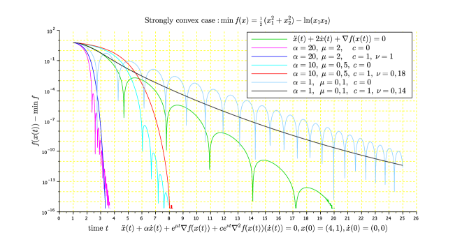
Figure 1: Evolution of $f(x(t))-\min f$ for solutions of (51), (52), and $f(x_{1},x_{2})=\frac{1}{2}\left(x_{1}^{2}+x_{2}^{2}\right)-\ln(x_{1}x_{2})$.

5.4 Numerical comparison

Figure 2 summarizes our convergence results, according to the behavior of the parameters $\gamma(t)$, $\beta(t)$, $b(t)$. Let’s comment on them and compare them, separately considering $f$ to be strongly convex or not.

$\gamma(t)$	$\beta(t)$	$b(t)$	$f(x(t))-\min f$	Reference
Cte	0	1	$\mathcal{O}\left(t^{-1}\right)$	(1964) polyak
Cte	Cte	1	$\mathcal{O}\left(t^{-1}\right)$	(2002) AABR
$\alpha/t$	0	1	$\mathcal{O}\left(t^{-\frac{2}{3}\alpha}\right)$ if $0<\alpha\leq 3$ $\mathcal{O}\left(t^{-2}\right)\;\;\;\;$ if $\alpha\geq 3$	(2019) att1 (2014) boyd
$\alpha/t$	Cte	1	$\mathcal{O}\left(t^{-2}\right)$ if $\alpha\geq 3,\beta>0$	(2016) APR
$\gamma(t)$	0	$b(t)$	$\mathcal{O}\left(\left(p(t)\int_{t}^{+\infty}(p(s))^{-1}ds\right)^{-2}(b(t))^{-1}\right)$ where $p(t):=\exp\left(\int_{t_{0}}^{t}\gamma(s)ds\right)$	(2019) att1
$\alpha/t$	$\beta(t)$	$b(t)$	$\mathcal{O}\left(\left(t^{2}b(t)-\dot{\beta}(t)-\dfrac{\beta(t)}{t}\right)^{-1}\right)$	(2020) ACFR

Figure 2: Convergence rate of $f(x(t))-\min f$ for instances of Theorem 2.1 and general $f$.

5.4.1 Strongly convex case

Suppose that $f$ is $s$-strongly convex. Following Polyak’s polyak , the system

$$\ddot{x}(t)+2\sqrt{s}\dot{x}(t)+\nabla f({x}(t))=0$$ (52)

provides the linear convergence rate $f(x(t))-\inf_{\mathcal{H}}f\leq Ce^{-\sqrt{s}t}$, see also (Siegel, , Theorem 2.2). In the presence of an additional Hessian-driven damping term

$$\ddot{x}(t)+2\sqrt{s}\dot{x}(t)+\beta\nabla^{2}f(x(t))\dot{x}(t)+\nabla f(x(t))=0\;\;\;(\beta\geq 0)$$ (53)

a related linear rate of convergence can be found in (ACFR, , Theorem 7). Let us insist on the fact that, in Corollary 3, we obtain a linear convergence rate for a general convex differentiable function $f$. In Figure 1, for the strongly convex function $f(x_{1},x_{2})=\frac{1}{2}\left(x_{1}^{2}+x_{2}^{2}\right)-\ln(x_{1}x_{2}),$ we can observe that some values of $\mu$ give a better speed of convergence of $f(x(t))-\min f$. We can also note that for $\mu$ correctly set, the system (51) provides a better linear convergence rate than the system (52).

5.4.2 Non-strongly convex case

We illustrate our results on the following simple example of a non strongly convex minimization problem, with non unique solutions.

$$\min_{{\mathbb{R}}^{2}}f(x_{1},x_{2})=\frac{1}{2}(x_{1}+10^{3}x_{2})^{2}.$$ (54)

From Figure 3 we get the following properties:
a) The convergence rate of the values is in accordance with Figure 2.
b) The system (51) is best for its linear convergence of values.
c) The Hessian-driven damping reduces the oscillations of the trajectories.

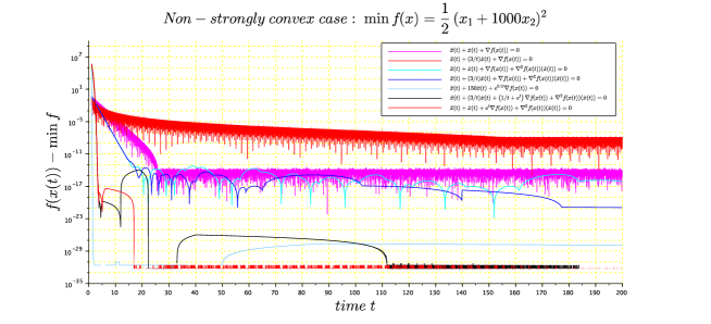
Figure 3: Evolution of $f(x(t))-\min f$ for systems in Figure 2, and $f(x_{1},x_{2})=\frac{1}{2}\left(x_{1}^{2}+10^{3}x_{2}^{2}\right)$.

6 Conclusion, perspectives

Our study is one of the first works to simultaneously consider the combination of three basic techniques for the design of fast converging inertial dynamics in convex optimization: general viscous damping (and especially asymptotic vanishing damping in relation to the Nesterov accelerated gradient method), Hessian-driven damping which has a spectacular effect on the reduction of the oscillatory aspects (especially for ill-conditionned minimization problems), and temporal rescaling. We have introduced a system of equations-inequations whose solutions provide the coefficients of a general Lyapunov functions for these dynamics. We have been able to encompass most of the existing results and find new solutions for this system, thus providing new Lyapunov functions. Also, we have been able to explain the mysterious coefficients which have been used in recent algorithmic developements, and which were just justified until now by the simplification of complicated calculations. Finally, by playing on fast rescaling methods, we have obtained linear convergence results for general convex functions. This work provides a basis for the development of corresponding algorithmic results.

References

- (1) F. Álvarez, On the minimizing property of a second-order dissipative system in Hilbert spaces, SIAM J. Control Optim., 38 (4) (2000), 1102-1119.
- (2) F. Álvarez, H. Attouch, J. Bolte, P. Redont, A second-order gradient-like dissipative dynamical system with Hessian-driven damping, J. Math. Pures Appl., 81 (2002), 747–779.
- (3) V. Apidopoulos, J.-F. Aujol, Ch. Dossal, Convergence rate of inertial Forward-Backward algorithm beyond Nesterov’s rule, Math. Program., 180 (2020) , 137–156.
- (4) H. Attouch, A. Cabot, Asymptotic stabilization of inertial gradient dynamics with time-dependent viscosity, J. Differential Equations, 263 (2017), 5412–5458.
- (5) H. Attouch, A., Cabot, Convergence rates of inertial forward-backward algorithms, SIAM J. Optim., 28 (2018), 849–874.
- (6) H. Attouch, A. Cabot, Z. Chbani, H. Riahi, Accelerated forward-backward algorithms with perturbations, J. Optim. Theory Appl., 179 (2018), 1–36.
- (7) H. Attouch, A. Cabot, Z. Chbani, H. Riahi, Rate of convergence of inertial gradient dynamics with time-dependent viscous damping coefficient, Evol. Equ. Control Theory, 7 (2018), 353–371.
- (8) H. Attouch, Z. Chbani, J. Fadili, H. Riahi, First-order optimization algorithms via inertial systems with Hessian driven damping, (2019) HAL-02193846.
- (9) H. Attouch, Z. Chbani, J. Peypouquet, P. Redont, Fast convergence of inertial dynamics and algorithms with asymptotic vanishing damping, Math. Program., (2019) DOI: 10.1007/s10107-016-0992-8.
- (10) H. Attouch, Z. Chbani, H. Riahi, Rate of convergence of the Nesterov accelerated gradient method in the subcritical case , ESAIM Control Optim. Calc. Var., 25(2) (2019), https://doi.org/10.1051/cocv/2017083
- (11) H. Attouch, Z. Chbani, H. Riahi, Fast proximal methods via time scaling of damped inertial dynamics, SIAM J. Optim., 29 (2019), 2227–2256.
-
(12)
H. Attouch, Z. Chbani, H. Riahi,