Localization transition, spectrum structure and winding numbers for one-dimensional non-Hermitian quasicrystals

Abstract

By analyzing the Lyapunov exponent (LE), we develop a rigorous, fundamental scheme for the study of general non-Hermitian quasicrystals with both complex phase factor and non-reciprocal hopping. Specially, the localization-delocalization transition point, $\mathcal{PT}$-symmetry-breaking point and the winding number transition points are determined by LEs of its dual Hermitian model. The analysis was based on Avila’s global theory, and we found that winding number is directly related to the acceleration, the slope of the LE, while quantization of acceleration is the crucial ingredient of Avila’s global theory. This result applies as well to the models with higher winding, not only the simplest Aubry-André model. As typical examples, we obtain the analytical phase boundaries of localization transition for non-Hermitian Aubry-André model in the whole parameter space, and the complete phase diagram is straightforwardly determined. For the non-Hermitian Soukoulis-Economou model, a high winding model, we show how the phase boundaries of localization transition and winding number transitions relate to the LEs of its dual Hermitian model. Moreover, we discover an intriguing feature of robust spectrum, i.e., the spectrum keeps invariant when one changes the complex phase parameter $h$ or non-reciprocal parameter $g$ in the region of $h<|h_{c}|$ or $g<|g_{c}|$ if the system is in the extended or localized state, respectively.

I Introduction

Localization induced by disorder is an old but everlasting research topic in condensed matter physics anderson1958absence . While Anderson localization induced by random disorder are thoroughly studied abrahams1979scaling ; lee1985disordered ; evers2008anderson ; Thouless72 , localization transition in quasiperiodic systems has attracted increasing interest in recent years luschen2018 ; Aubry1980 ; Kohmoto1983 ; Thouless1988 ; roati2008 . In comparison with the random disorder systems, the quasiperiodic systems manifest some peculiar properties and may support exact results due to the existence of duality relation for the transformation between lattice and momentum spaces. A typical example is the Aubry-André (AA) model Aubry1980 , which undergoes a localization transition when the quasiperiodical potential strength exceeds a transition point determined by a self-duality condition Jitomirskaya1999 . Various extensions of AA models have been studied Kohmoto1983 ; Ceccatto ; Zhou2013 ; Cai ; DeGottardi ; Kohmoto2008 ; WangYC-review ; Chandran ; Chong2015 . The quasiperiodic lattice models can support energy-dependent mobility edges when either short-range (long-range) hopping processes biddle2011localization ; biddle2010predicted ; ganeshan2015nearest ; li2016quantum ; li2017mobility ; li2018mobility ; DengX or modified quasiperiodic potentials sarma1988mobility ; sarma1990localization ; YCWang2020 are introduced.

The interplay of non-Hermiticity and disorder brings new perspective for the localization phenomena. Due to the releasing of the Hermiticity constrain, non-Hermitian random matrices contain much more rich symmetry classes according to Bernard-LeClair classification BL ; HYZhou ; CHLiu ; Sato than the corresponding Hermitian Altland-Zirnbauer classification. In the scheme of random matrix theory, it has been demonstrated that the spectral statistics for non-Hermitian disorder systems displays many different features from the Hermitian systems Goldsheid ; Markum ; Molinari ; Chalker ; Shindou ; Ueda-RM ; XRWang ; Ryu . The interplay of the nonreciprocal hopping and random disorder has been studied in terms of the Hatano-Nelson-type models hatano1996localization ; hatano1998non ; kolesnikov2000localization ; Gong ; ZhangDW ; Hughes . The effect of complex disorder potentials has also been investigated HuangYi ; ZhangDW2 ; Tzortzakakis . Non-Hermitian quasiperiodic systems have also attracted intensive studies very recently Yuce ; longhi2019metal ; jazaeri2001localization ; jiang2019interplay ; zeng2019topological ; longhiPRL ; ZengQB ; Zeng2020 ; Liutong ; Liu2020 ; Liu2020L ; Cai2021AA ; Longhi2021AA ; Zhai2020 ; Liu2020DM ; Tang2021TO ; Cai2021PW .

The LE is an important quantity to characterize the localization properties of disorder systems and plays an essential role in the study of localization transition. As one of Avila’s Fields Medal work, he developed global theory of quasiperiodic cocycles and studied the delicate but fundamental property of LE. This is quite an important progress in the spectral theory of self-adjoint quasiperiodic Schrödinger operators Avila2015 ; Avila2017 . Nevertheless, the application of the global theory to the study of physical properties of quasiperiodic systems is not well recognized in the physics communities. Particularly, the study of non-Hermitian quasicrystals in terms of the global theory was only addressed very recently Liu2020L , and a systematic scheme applicable for general non-Hermitian quasiperiodic systems is not established yet. The studies of the general non-Hermitian quasiperiodic models with high winding number are neglected due to the lack of the exact transition points and universal formulas. In this paper, we develop a fundamental scheme for the study of general non-Hermitian quasiperiodic systems by applying Avila’s global theory, where the non-Hermitian systems can be realized by introducing both non-reciprocal hopping and complex phase factor in the Hermitian quasiperiodic model. We find some universal results to determine the localization-delocalization transition point, $\mathcal{PT}$-symmetry-breaking point and the winding number transition points. For the case in presence of complex phase factor, the picture of LE actually gives us the mechanism of how winding number and localized phase change with complex phase factor. It is surprising that the relevant information for the non-Hermitian systems can be acquired from their dual Hermitian models. For the case in presence of non-reciprocal hopping, the skin effect-localization transition and winding number transition are also directly related to LEs.

We stress that our theory and formalism are valid for general non-Hermitian quasiperiodic systems. For a better understanding, our general theory is made concrete by focusing on two typical examples, i.e., non-Hermitian AA model and Soukoulis-Economou model, as showcases for presenting the main results. Despite its deceptively simple form, the phase boundaries of localization-delocalization transition of the general non-Hermitian AA model are still not known, except of two limit cases in the absence of either non-reciprocal hopping longhiPRL and complex potential jiang2019interplay . A complete phase diagram with analytical phase boundaries in the full parameter space is lacking. In addition, although the coincidence of localization transition point with the $\mathcal{PT}$-symmetry-breaking point in the $\mathcal{PT}$-symmetry AA model has been numerically observed longhiPRL , no analytical proof is given.We shall clarify these issues by applying our general scheme. Some unusual and unexplored spectrum features of non-Hermitian AA models, i.e., the spectra are invariant with the change of complex phase parameter $h$ or non-reciprocal parameter $g$ in specific regions, are also unveiled. The feature of robust spectra is found to exist very commonly in non-Hermitian quasiperiodic systems.

The paper is organized as follows. In section II, we first introduce the general model and present the formalism of our general theory. We start from the systems with complex quasiperiodic potential in the subsection II.A, and demonstrate that the localization-delocalization transition point for general non-Hermitian quasicrystals with complex phase factor can be determined by LEs of its dual Hermitian model. Under the general framework, both the complex AA model and Soukoulis-Economou model are studied. Then we study the general case in the presence of nonreciprocal hopping in the subsection II.B. Taking the non-Hermitian AA model as a typical example, we obtain the complete phase diagram which is determined by an analytical formula for the localization transition point. In section III, We study the properties of winding numbers and relate them directly to the slope of LEs. Then we identify that the phase diagram of non-Hermitian quasiperiodic models can be characterized by winding numbers. In section IV, we study the properties of robust spectrum and skin effect. The invariance of spectrum structure of non-Hermitian AA model under the change of $h$ or $g$ in specific regions are studied and analyzed. Then we study the interplay of skin effect and localization and demonstrate that the sensitivity of spectrum structures to the change of boundary condition from periodic to open boundary condition (PBC to OBC) can distinguish the skin and localized phases. In section V, we give some examples beyond the AA model and Soukoulis-Economou model. A summary is given in the final section.

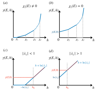
Figure 1: Schematic representation of Eq. (11): the LE $\gamma(E,h)$ as a function of $h$ for (a) $\chi\neq 0$ and (b) $\chi=0$, respectively. For the AA model, the LE $\gamma(E,h)$ with (c) $|\lambda_{1}|<1$ and (d) $|\lambda_{1}|>1$, respectively.

II Models and general theory

We consider the general non-Hermitian quasiperiodic models with both complex potential and non-reciprocal hopping, described by

$$H=\sum_{j=1}^{N}\left(t_{L}|j\rangle\left\langle j+1\right|+t_{R}\left|j+1\right\rangle\langle j|+V_{j}|j\rangle\langle j|\right),$$ (1)

where $t_{L}=te^{-g}$ and $t_{R}=te^{g}$ are the left-hopping and right-hopping amplitude, respectively, $V_{j}$ is given by

$$V_{j}=\sum_{l=1}^{d}2\lambda_{l}\cos[l(2\pi\omega j+\theta)],$$ (2)

with

$$\theta=\phi+ih$$

describing a complex phase factor, and $N$ is the lattice size. For convenience, we set $t=1$ as the unit of energy and take $\omega=\left(\sqrt{5}-1\right)/2$, which can be approached by $\omega=\lim_{n\rightarrow\infty}\frac{F_{n-1}}{F_{n}}$ with the Fibonacci numbers $F_{n}$ defined recursively by $F_{n+1}=F_{n}+F_{n-1}$ and $F_{0}=F_{1}=1$. By taking $|\psi\rangle=\sum_{j}u_{j}|j\rangle$, the eigen equation is given by

$$Eu_{j}=e^{-g}u_{j+1}+e^{g}u_{j-1}+V_{j}u_{j},$$ (3)

where the eigenvalue $E$ is generally complex.

II.1 Models with complex quasiperiodic potential

We first discuss the case in the absence of non-reciprocal hopping, i.e., $g=0$. For $\phi=0$, we have $V_{j}=V^{*}_{-j}$, the model (1) with $g=0$ has $\mathcal{PT}$ symmetryBender ; Yuce . Our whole analysis depends on Avila’s global theory of quasi-periodic Schrödinger operator Avila2015 (see Appendix A for brief introduction), where the key is to analysis the LE $\gamma\left(E,h\right)$ with respect to $h$. The LE is given by

$$\gamma\left(E\right)=\lim_{n\rightarrow\infty}\frac{1}{n}\ln\left|\left|T_{n}\left(E\right)\right|\right|,$$ (4)

where the transfer matrix

$$T_{n}\left(E\right)=\prod_{j=1}^{n}T^{j}=\prod_{j=1}^{n}\left(\begin{array}[]{cc}E-V_{j}&-1\\ 1&0\end{array}\right)$$ (5)

and $\left|\left|A\right|\right|$ represents the norm of the matrix $A$, defined by

$$\left|\left|A\right|\right|=max_{i=1:n}\sqrt{\lambda_{i}(A^{T}A)}$$

with $\lambda_{i}(A^{T}A)$ being the $i$-th eigenvalue of $A^{T}A$.

As shown in Avila2015 , $\gamma\left(E,h\right)$ is a convex and piece-wise linear function with respect to $h$ with their slopes being integers. If $V_{j}$ is trigonometric polynomial (i.e. $d<\infty$), then the extreme points of $\gamma\left(E,h\right)$ can be determined by the LE of corresponding dual Hermitian Hamiltonian GJYZ . More precisely, it has the following expansion:

$$\gamma\left(E,h\right)=\left\{\begin{array}[]{cc}\gamma(E,0),{}{}&h\in[0,\chi_{1}(E)],\\ \vdots&\vdots\\ \gamma(E,\chi_{i}(E))+(h-\chi_{i}(E))\sum_{j=1}^{i}{n_{j}},&~{}~{}h\in(\chi_{i}(E),\chi_{i+1}(E)],\\ \vdots&\vdots\\ \gamma(E,\chi_{\ell}(E))+(h-\chi_{l}(E))\sum_{j=1}^{\ell}{n_{j}},&~{}~{}h\in(\chi_{\ell}(E),\infty),\end{array}\right.$$ (11)

where $0\leq\chi_{1}(E)<\cdots<\chi_{\ell}(E)$ are the non-negative LEs with multiplicity $n_{1},\cdots,n_{\ell}$ for the dual model of the system (1) with $h=0$

$$E\tilde{u}_{k}=\sum\limits_{l=-d}^{d}\lambda_{|l|}\tilde{u}_{k+l}+2\cos(2\pi\omega k)\tilde{u}_{k}.$$ (12)

This means that the LE $\gamma\left(E,h\right)$ can be uniquely determined by $\gamma(E,0)$, $\chi_{i}$ and $n_{i}$. These points $h=\chi_{i}$ are knotted, which correspond to some physical consequence. However, we emphasize that duality is not the essence of our approach. The crucial things are the extreme point and the slope of $\gamma\left(E,h\right)$, and duality only gives an efficient way to achieve these parameters. That is also the reason why our approach works for general non-Hermitian quasiperiodic models (c.f. Section V). We also should point out that in the following discussion, we only need to consider the case $E$ belong to the spectrum of the Hermitian case($h=0$). Actually, based on Avila’s global theory, we can get that if $E$ doesn’t belong to the spectrum of the Hermitian case, $\gamma\left(E,0\right)>0$ and $\chi_{1}(E)>0$. To better understand the Eq. (11), we show the LE $\gamma\left(E,h\right)$ in Fig 1 (a) and (b) as a function of $h$ with $h>0$. Note that $\gamma(E,h)$ is symmetric over $h$, i.e.,

$$\gamma(E,h)=\gamma(E,-h).$$ (13)

An intriguing issue is that the $\mathcal{PT}$-symmetry breaking transition and the transition from extended to localized states can be both determined by the LE of Hermitian dual model $\chi_{1}(E)$. To explain it clearly, we will start with the representative model, the AA model, i.e., only $\lambda_{1}\neq 0$, which is discussed in detail in the following. The dual model form for the model (1) with $g=0$, $h=0$ and $\lambda_{l\geqslant 2}=0$ is

$$E\tilde{u}_{k}=\lambda_{1}\tilde{u}_{k+1}+\lambda_{1}\tilde{u}_{k-1}+2\cos(2\pi\omega k)\tilde{u}_{k},$$ (14)

The exact LE $\chi\left(E\right)$ of this dual model can be obtained by Eq. (4) with the transfer matrix $T_{n}$ is given by

$$T_{n}\left(E\right)=\prod_{j=1}^{n}T^{j}=\prod_{j=1}^{n}\left(\begin{array}[]{cc}\frac{E-2\cos(2\pi\omega k)}{\lambda_{1}}&-1\\ 1&0\end{array}\right).$$ (15)

From the discussions in Avila2015 ; YCWang2020 , we have

$$\chi(E)=\max\{-\ln|\lambda_{1}|,0\},$$ (16)

if the energy $E$ belongs to the spectrum. Thus the LE for the original model with $h\neq 0$ can be written as

$$\gamma\left(E,h\right)=\left\{\begin{array}[]{cc}\gamma\left(E,0\right),&h\in[0,\chi(E)],\\ \gamma\left(E,\chi(E)\right)+(h-\chi(E)),&h\in(\chi(E),\infty),\end{array}\right.$$ (19)

which can be also rewritten as

$$\gamma(E,h)=\max\{\ln|\lambda_{1}|+|h|,0\}.$$ (20)

The LE can be also directly derived from the original model (see Appendix A.1) without the need to introduce the dual model.

Figs.1(c) and (d) show the LE $\gamma(E,h)$ for non-critical AA models with $|\lambda_{1}|<1$ and $|\lambda_{1}|>1$, respectively. Note $\gamma\left(E,h\right)=0$ indicates the extended state, and $\gamma\left(E,h\right)>0$ corresponds the localized state. Thus if $|\lambda_{1}|<1$, all the eigenstates of Hermitian AA model ($h=0$) are extended. When $|h|>0$, there exists a localization-delocalization transition point determined by

$$|h|=-\ln|\lambda_{1}|.$$ (21)

If $|\lambda_{1}|>1$, all the eigenstates of Hermitian AA model are localized and all the eigenstates stay localized with $|h|>0$.

In the following, we first consider the case $|\lambda_{1}|<1$. For simplicity, we only discuss the case $h>0$. By Avila’s global theory Avila2015 , $E$ does not lie in the spectrum of the Hamiltonian $h=h_{0}$, if and only if $\gamma(E,h_{0})>0$, and $\gamma(E,h)$ is a linear function around $h_{0}$. Therefore, if $E$ lies in the spectrum of the Hermitian case $h=0$, it belongs to the spectrum of the system with $h<-\ln|\lambda_{1}|$, but does not belong to the spectrum of the system with $h>-\ln|\lambda_{1}|$, as shown in the blue dashed line of Fig.1 (c). Conversely, if the energy $E$ (might be complex) doesn’t lie in the spectrum of the Hermitian case $h=0$, then $\gamma(E,0)>0$ and $\gamma(E,h)$ is locally constant in $h$, as shown in the red dashed line of Fig.1 (c). Note that $h_{0}$ is an extreme point of $\gamma(E,h)$ if and only if $h_{0}>-\ln|\lambda_{1}|$. Therefore these energies $E$ do not belong to the spectrum of the system with $h<-\ln|\lambda_{1}|$, which might belong to the spectrum of the system with $h>-\ln|\lambda_{1}|$. By the above discussions, we prove that the extended states have real energies when $h<-\ln|\lambda_{1}|$, and the localized states have complex eigenvalues when $h>-\ln|\lambda_{1}|$. This explains why the localization transition point coincides with the $\mathcal{PT}$-symmetry breaking point. Furthermore, the spectrum keeps invariant in the regime of extended states, which is indeed a Cantor set by famous result of Avila-Jitomirskaya Avila .

However, the case $|\lambda_{1}|>1$ will be much simpler. By similar discussion as above, one can easily deduce that when $h>0$, all the sates are localized, which have complex eigenvalues, as shown in Fig.1 (d).

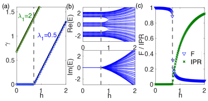
Figure 2: (a) Numerical results for the LE of eigenstates corresponding to the minimum (circles) and maximum(dots) real part of eigenvalues Re$(E)$ versus $h$ for the system with $g=0$, $N=1597$, $\lambda=0.5$ and $2$, respectively. The black solid lines represent the exact solution of the LE obtained by (20). (b) The real and the imaginary part of the eigenvalue spectra versus $h$ for the system with $\lambda_{1}=0.5$, $g=0$ and $N=55$. (c) The fidelity $F$ and IPR of eigenstate corresponding to the minimum real part of eigenvalues Re$(E)$ versus $h$ for the system with $g=0$, $N=1597$, and $\lambda_{1}=0.5$.

To get a straightforward understanding, next we demonstrate numerical results of LE, inverse participation ratio (IPR), the normalized participation ratio (NPR)li2016quantum ; li2018mobility ; li2017mobility and energy spectrum as a function of $h$. For a finite system, the LE can be numerically calculated via

$$\gamma\left(E\right)=\ln\left(\max\left(\theta_{i}^{+},\theta_{i}^{-}\right)\right),$$ (22)

where $\theta_{i}^{\pm}\in\mathbb{R}$ denote eigenvalues of the matrix

$$\mathbf{\Theta=}\left(T_{N}^{{\dagger}}T_{N}\right)^{1/(2N)}.$$ (23)

The IPR and NPR of an eigenstate is defined as

$$\text{IPR}^{(n)}=(\sum_{j}\left|u_{j}^{n}\right|^{4})/\left(\sum_{j}\left|u_{j}^{n}\right|^{2}\right)^{2},$$

and

$${\rm NPR}^{(n)}=\left[N\sum_{i}|u_{i}^{n}|^{4}\right]^{-1},$$ (24)

where the superscript $n$ labels the $n$th eigenstate of system, and $j$ represents the lattice coordinate. For an extended eigenstate, IPR$\simeq 1/N$ approaches zero as $N\rightarrow\infty$ and NPR is a finite value. On the other hand, IPR$\simeq 1$ and NPR$\simeq 0$ for a full localized eigenstate.

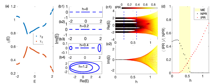
Figure 3: (a) The LE of the dual model with $\lambda_{1}=0.2$ and $\lambda_{2}=0.25$. (b) The complex spectrum for systems with (b1) $h=0$, (b2) $0.2$, (b3) $0.4$ and (b4) $1.1$, respectively. (c)The real and imaginary part of the eigenvalue spectra versus $h$ for the system with $g=0$, $\lambda_{1}=0.2$, and $\lambda_{2}=0.25$. Dashed blue lines indicate the transition point: $h_{1}=0.23$ and $h_{2}=0.6$. (d) Averaged IPR and NPR for all eigenstates in the model.

Figs.2 (a) and (c) show the numerical results of the LE and IPR versus $h$, respectively. If $|\lambda_{1}|<1$, when $|h|<\chi(E)$, where $\chi(E)=-\ln|\lambda_{1}|\approx 0.7$ for $\lambda_{1}=0.5$, all eigenstates are extended states and both LE and IPR approach zero. on the other hand, when $h>\chi(E)$, both LE and IPR have a sudden increase. If $|\lambda_{1}|>1$, all eigenstates are localized, as shown in the Fig.2(a) with $\lambda_{1}=2$. The numerical results of LE for finite size system are found to agree well with the analytical result (20). In Fig.2(b), we display the real and imaginary part of eigenvalues versus $h$ for the system with $\lambda_{1}=0.5$. While all eigenvalues are real for $h<\chi(E)$, they become complex when $h$ exceeds $\chi(E)$. This clearly shows that the transition from extended to localized states and $\mathcal{PT}$-symmetry breaking transition have the same boundary.

It is also interesting to notice that the spectrum does not change with $h$ in the extended region as long as $h<\chi(E)$. This kind of phenomenon is quite unusual, since the Hamiltonian with different $h$ is not unitary equivalent, and it’s just kind of robust spectrum. The similarity of two eigenstates can be characterized by the fidelity

$$F(h)=\langle\psi_{g}(0)|\psi_{g}(h)\rangle,$$ (25)

where $\psi_{g}(h)$ is the eigenstate of corresponding the minimum real part of eigenvalue, and $\psi_{g}(0)$ with $h=0$. The eigenstates vary only slightly from $h=0$ to $h<\chi(E)$, and change suddenly at the transition point $h=\chi(E)$, as shown in Fig. 2(c).

Although, the above phenomenons show in a simple case, these phenomenons can be commonly found in general non-Hermitian quasiperiodic models (1) with $g=0$. If $\chi_{1}(E)=0$, which means $\gamma(E,0)>0$, there is no extended-localized transition for complex phase $h>0$. We thus only need to consider the case $\chi_{1}(E)>0$. If $0<h<\chi_{1}(E)$ for a given eigenvalue $E$ of the system with $h=0$, the eigenvalue remains unchanged and the corresponding eigenstate is extended. If $h>\chi_{1}(E)$, the eigenvalue becomes complex and the corresponding eigenstate is localized. As a consequence, $h=\min\{\chi_{1}(E)\}$ gives the beginning of $\mathcal{PT}$ symmetry breaking and extended-mixed transition, while $h=\max\{\chi_{1}(E)\}$ gives us the mixed-localized transition. That is to say, if $\min\{\chi_{1}(E)\}<h<\max\{\chi_{1}(E)\}$, the mobility edges will occur, the spectrum will have both real and complex energies, and the phases will be mixture of extended and localized states. Moreover, if $0<h<\min\{\chi_{1}(E)\}$, the spectrum is exactly the same as the Hermitian case $h=0$, thus has robust spectrum when changing $h$. Just note that if $\min\{\chi_{1}(E)\}=\max\{\chi_{1}(E)\}$ or say $\chi_{1}(E)$ is a constant, then $h=\min\{\chi_{1}(E)\}$ gives the extended-localized transition point, just as the non-Hermitian AA model. Finally, we point out $\chi_{1}(E)$ is also the inverse of localization length of the eigenstate for the Hermitian dual model (12), and if $\chi_{1}(E)>0$, the corresponding eigenstate of system (12) is localized.

Next we will demonstrate this with Soukoulis-Economou model Soukoulis , one of the first proposals of one-dimensional quasiperiodic models containing single-particle mobility edges. It is a tight-binding model with nearest-neighbor hopping terms as well as two quasiperiodic on-site potentials:

$$V_{j}=2\lambda_{1}\cos(2\pi\omega j+ih)+2\lambda_{2}\cos(4\pi\omega j+2ih).$$ (26)

Our analysis shows that the mobility edge for the system with any $h$ can be determined by the LE $\chi_{1}(E)$ for its dual Hermitian system (12).

For the potential (26) with $h=0$, its dual model (12) is

$$E\tilde{u}_{k}=\lambda_{1}(\tilde{u}_{k+1}+\tilde{u}_{k-1})+\lambda_{2}(\tilde{u}_{k+2}+\tilde{u}_{k-2})+2\cos(2\pi\omega k)\tilde{u}_{k},$$ (27)

and $\tilde{u}_{k}=\sum_{n}e^{-i2\pi\omega kj}u_{j}.$ We can rewrite (27) as

$$\left(\begin{array}[]{c}\tilde{u}_{k+3}\\ \tilde{u}_{k+2}\\ \tilde{u}_{k+1}\\ \tilde{u}_{k}\\ \end{array}\right)=T^{k}\left(\begin{array}[]{c}\tilde{u}_{k+1}\\ \tilde{u}_{k}\\ \tilde{u}_{k-1}\\ \tilde{u}_{k-2}\\ \end{array}\right),$$

with

$$T^{k}=\left(\begin{array}[]{cc}C_{2}^{-1}(EI_{2}-B_{2})&-C_{2}^{-1}C_{2}^{*}\\ I_{2}&0\\ \end{array}\right),$$

where $I_{2}$ is the $2\times 2$ identity matrix, the matrices $C_{2}$ and $B_{2}$ are given by

$$C_{2}=\left(\begin{array}[]{cc}\lambda_{2}&\lambda_{1}\\ 0&\lambda_{2}\\ \end{array}\right),$$

and

$$B_{2}=\left(\begin{array}[]{cc}2\cos(2\pi\omega(k+1))&\lambda_{1}\\ \lambda_{1}&2\cos(2\pi\omega k)\\ \end{array}\right).$$

Denote the transfer matrix $T_{n}(E)=\prod_{k}T^{k}$, then the LEs of the model (27) are given by

$$\chi_{i}=\ln\theta_{i},$$ (28)

where $\theta_{i}$ are the eigenvalues of matrix

$$\mathbf{\Theta}=\left(T_{N}^{{\dagger}}T_{N}\right)^{1/(2N)}.$$

Since $T^{k}$ is a $4\times 4$ complex symplectic matrix, their LEs (28) come in pairs, and we write it as $-\chi_{2}(E)\leq-\chi_{1}(E)\leq 0\leq\chi_{1}(E)\leq\chi_{2}(E)$. The LE (11) for the original model with $d=2$ and $h\neq 0$ can be written as

$$\gamma\left(E,h\right)=\left\{\begin{array}[]{cc}\gamma\left(E,0\right),&~{}~{}h\in[0,\chi_{1}(E)],\\ \gamma\left(E,\chi_{1}(E)\right)+(h-\chi_{1}(E)),&~{}~{}h\in(\chi_{1}(E),\chi_{2}(E)],\\ \gamma\left(E,\chi_{2}(E)\right)+2(h-\chi_{2}(E)),&~{}~{}h\in(\chi_{2}(E),\infty).\end{array}\right.$$ (32)

Fig. 3(a) shows the LEs $\chi_{1}(E)$ and $\chi_{2}(E)$ of the dual model (27) with $\lambda_{1}=0.2$ and $\lambda_{2}=0.25$ as a function of eigennergy $E$, and in Fig.3(b) and (c), we display its spectrum versus $h$. We also show the averaged IPR and NPR in Fig.3(d) to distinguish these phases. From these pictures, it is clear that the spectrum keeps invariant in the region of $h<h_{1}$, where $h_{1}=\min\{\chi_{1}(E)\}=0.23$ is also the $\mathcal{PT}$-symmetry breaking point, all the eigenvalues are real and all the eigenstates are extended. The mobility edge region $h_{1}<h<h_{2}$ represents the system with a mixture of localized and extended states, where $h_{2}=\max\{(\chi_{1}(E)\}=0.6$. The extended states have real eigenvalues, while the localized states have complex eigenvalues, as shown in Fig.3 (b3) and (c). Eventually, when $h>h_{2}$, all the eigenstates are localized, and their corresponding eigenvalues are complex. Our results clearly indicate that the three distinct phases can be divided by $h=\max\{\chi_{1}(E)\}$ and $h=\max\{\chi_{1}(E)\}$.

II.2 Effect of non-reciprocal hopping

Now we consider the general case with $g\neq 0$. The nonreciprocal hopping breaks the $\mathcal{PT}$ symmetry and may induce skin effect under OBC. The Hamiltonian $H(g)$ under OBC can be transformed to $H^{\prime}$ via a similar transformation

$$H^{\prime}=SH(g)S^{-1},$$ (33)

where

$$S=\text{diag}\left(e^{-g},e^{-2g},\cdots,e^{-Ng}\right)$$

is a similarity matrix with only diagonal entries and $H^{\prime}=H(g=0)$ is the Hamiltonian with $g=0$. The eigenvectors of $H$ and $H^{\prime}$ satisfy $\left|\psi\right\rangle=S^{-1}\left|\psi^{\prime}\right\rangle$. An extended state $\left|\psi^{\prime}\right\rangle$ under the transformation $S^{-1}$ becomes skin states, which exponentially accumulate to one of boundaries jiang2019interplay ; Yao ; Kunst ; Alvarez ; Xiong ; Lee .

A localized state of $H^{\prime}$ generally takes the following form

$$\left|u_{i}\right|\propto e^{-\left|i-i_{0}\right|/\xi},$$

where $i_{0}$ represents the position of localization center of a given localized state, $\xi=1/\gamma$ is the localization length, and $\gamma$ is the LE of the localized state for the system with $g=0$. Then the corresponding wavefunction of $H(g)$ takes the following form:

$$\left|u_{i}\right|\propto\left\{\begin{array}[]{cc}e^{-\left(\gamma-g\right)\left|i-i_{0}\right|}&i>i_{0}\\ e^{-\left(\gamma+g\right)\left|i-i_{0}\right|}&i<i_{0}\end{array}\right.,$$ (34)

which has different decaying behaviors on different sides of the localization center. When $\left|g\right|\geq\gamma$, delocalization occurs on one side and then skin state emerges to the boundary. The transition point from the localized state to skin state is given by

$$\gamma(E)=\left|g\right|.$$ (35)

Since a localized state is not sensitive to the boundary condition of the system, we conclude that the boundary of localization-delocalization transition under the PBC is also given by Eq.(35).

For general Hermitian quasi-periodic model (1), LEs might depend on $E$, and mobility edge will occur. Consequently, if $g\neq 0$, Eq. (35) gives the mobility edge from the localized state to extended (skin) state. The localized eigenstate in the case $g=0$ is still localized when $0<g<\gamma(E)$. However, the localized eigenstate becomes extended (skin) under the PBC (OBC), when $g>\gamma(E)$.

For the non-Hermitian AA model with $h\neq 0$ and $g=0$, the LEs of the localized states are given by $\gamma=|h|+\ln|\lambda_{1}|$, according to Eq.(20). Thus if $g\neq 0$, by using Eq.(35), the localization transition boundary is determined by

$$\left|h\right|+\ln\left|\lambda_{1}\right|=\left|g\right|,$$ (36)

which can be alternatively represented as

$$|\lambda_{1}|=e^{-|h|+|g|}.$$ (37)

While all eigenstates are localized for $|\lambda_{1}|>e^{-|h|+|g|}$, they become extended (skin) states under PBC (OBC) for $|\lambda_{1}|<e^{-|h|+|g|}$. The model reduces to the classical AA model when $h=0$ and $g=0$. Eq.(37) recovers the result of Ref.longhiPRL for $h\neq 0$ and $g=0$ and the result of Ref.jiang2019interplay for $g\neq 0$ and $h=0$.

By using either Eq.(36) or Eq.(37), we can obtain the complete phase diagram. For a given $\lambda_{1}$, we display the phase diagram in Fig.4 with the phase boundaries (solid lines) determined by Eq.(36). Fig. 4(a) and 4(b) correspond to the case $\lambda_{1}<1$ and $\lambda_{1}>1$, respectively. Here regions labeled by $A$ denote the Anderson localized phase, and regions labeled by $L$ or $R$ represent the left or right skin states under OBC, which are extended phase under PBC. From the phase diagrams, we can see that, while increasing $|h|$ tends to driving the system into localized phase, increasing $|g|$ tends to driving the system into extended (skin) phase. When $|h|=|g|$, the transition point is given by $\lambda_{c}=1$, which is irrelevant to the values of $h$ and $g$, and eigenstates for system with $\lambda_{1}<1$ ($\lambda_{1}>1$) are extended (localized).

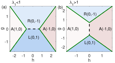
Figure 4: Phase diagrams for the case with (a) $|\lambda_{1}|<1$ and (b) $|\lambda_{1}|>1$, respectively. The phase boundaries are denoted by the green solid lines, which are determined by $|g|=\ln|\lambda_{1}|+|h|$. The winding numbers ($\nu_{\phi},\nu_{\psi}$) are defined in the text. $\{L,R,A\}$ represent the left-skin, right-skin, and Anderson localized phases, respectively. The left-skin and right-skin phases under OBC correspond to extended phases under PBC. We have taken $\lambda_{1}=0.5$ in (a) and $\lambda_{1}=2$ in (b).

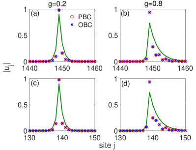
Figure 5: The distribution of eigenstates for systems with $\lambda_{1}=2$, $h=0.5$, $N=1597$, $g=0.2$ and $0.8$, respectively. The red circles and blue crosses represent the eigenvalues under PBC and OBC, respectively. The solid line is plotted by using Eq. (34). The localization centers for states shown in (a) and (b) are at $j=1449$, and for (c) and (d) are at $j=139$.

For the AA model, the LE of the localized state is independent of $E$. This suggests that all eigenstates are either localized or extended (skin) states with the transition point independent of $E$. Also, we can conclude that all localized states of non-Hermitian AA model can be described by a unified wavefuntion (34) with different states having different localization centers, as shown in Figs. 5(a) and (c) or Figs. 5(b) and (d).

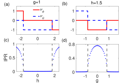
Figure 6: The winding number $\nu_{\phi}$, $\nu_{\psi}$ versus $h$ for the system with $g=1$ (a) and versus $g$ for the system with $h=1.5$ (b). The IPR of eigenstates corresponding to the middlemost real part of eigenvalue Re$(E)$ versus $h$ for the system with $g=1$ (c) and versus $g$ for the system with $h=1.5$ (d). Other parameters are $\lambda_{1}=0.5$ and $N=233$, and we have taken PBC in the numerical calculations.

III Winding numbers

The phase factor $\phi$ of the potential provides a parameter space to define topological invariant, i.e. the winding number, to characterize the topological phase of the non-Hermitian quasiperiodic system. Changing the complex phase $h$ may induce topological phase transition. Recall that the winding number of the system can be defined as

$$\nu_{\phi}=\frac{1}{2\pi i}\frac{1}{N}\int_{0}^{2\pi}\text{d}\phi\partial_{\phi}\ln\det[H(\phi)-E_{B}],$$ (38)

which measures the change of spectrum with respect to the base energy $E_{B}$ when $\phi$ is changed continuously. Thus it is interesting to know where does the topological transition occur? Indeed, this question can also be answered with the help of LE. As we explained above, the slope of LE, which is called acceleration Avila2015 is quantized. We will show that quantization of the winding number just means the acceleration is quantized.

Let us explain in more details. In the case $g=0$, as we show in the Appendix B, based on Cauchy-Riemann equation, we have the following relation

$$\nu_{\phi}(E,h)=-\frac{\partial\gamma(E,h)}{\partial h}.$$ (39)

Here $\frac{\partial\gamma(E,h)}{\partial h}$ is exactly the “acceleration” as defined by Avila Avila2015 . Note $\gamma\left(E,h\right)$ is a piece-wise linear function with respect to $h$ with their slopes being integers, then acceleration is just the slope. In the following sections, we only need to consider $h>0$. Due to the symmetry (13), $\nu_{\phi}(E,h)$ always satisfies

$$\nu_{\phi}(E,-h)=-\nu_{\phi}(E,h).$$ (40)

If $g\neq 0$, then boundary conditions make things different. Under PBC, we will show that

$$\nu_{\phi}(E,h,g)=\left\{\begin{array}[]{cc}0,&~{}|g|>\gamma(E,h)\\ -\frac{\partial\gamma(E,h)}{\partial h},&~{}0<|g|<\gamma(E,h)\end{array}\right..$$ (41)

However, within OBC, we have

$$\nu_{\phi}(E,h,g)=\nu_{\phi}(E,h)=-\frac{\partial\gamma(E,h)}{\partial h},$$ (42)

for any $g\neq 0$. The Eqs. (41) and (42) are strictly educed in Appendix B. The different boundary conditions correspond to the different winding number, which can also be interpreted as a phenomenon for breakdown of bulk-boundary correspondence.

Based on Eqs.(11), (39) and (41), our analysis really shows the topological transition of general non-Hermitian quasiperiodic models, that is to say, the transition point is also determined by the LE $\chi_{i}(E)$ of the dual model (12). For simplicity, we will just demonstrate this with AA model and Soukoulis-Economou model.

For the non-Hermitian AA model, when $\lambda_{1}<1$, the Eqs. (39) and (41) can be expressed as

$$\nu_{\phi}(E,h)=\left\{\begin{array}[]{cc}0,&~{}h<-\ln|\lambda_{1}|,\\ -1,&~{}h>-\ln|\lambda_{1}|,\end{array}\right.$$ (43)

and

$$\nu_{\phi}(E,h,g)=\left\{\begin{array}[]{cc}0,&~{}g>h+\ln|\lambda_{1}|,\\ -1,&~{}g<h+\ln|\lambda_{1}|,\end{array}\right.$$ (44)

based on Eq.(20). In Fig.6, we show how the winding numbers and IPR change with $h$ or $g$. Fig. 6(a) and (c) are for the system with fixed $\lambda_{1}=0.5$ and $g=1$. According to Eq.(35), we have $|h_{c}|=|g|-\ln|\lambda_{1}|\approx 1.7$. It is shown that the winding number $\nu_{\phi}$ takes different integer $0$ or $\pm 1$ in the region $|h|<1.7$ or $|h|>1.7$, and IPR shows that the corresponding states are extended or localized. Fig.6(b) and (d) show the winding numbers $\nu_{\phi}$ and IPR of the system with $\lambda_{1}=0.5$ and $h=1.5$ versus $g$. According to Eq.(35), we have $|g_{c}|=|h|+\ln|\lambda_{1}|\approx 0.8$. The winding number $\nu_{\phi}$ takes different integer $0$ or $-1$ in the region $|g|<0.8$ or $|g|>0.8$, and IPR shows that the corresponding states are localized or extended. The numerical results clearly indicate that the winding number changes its value when crossing the boundary of localization transition and takes different integer in extended and localized regions. Consequently, we also show that different phases in the phase diagram of Fig.4 can be characterized by different $\nu_{\phi}$.

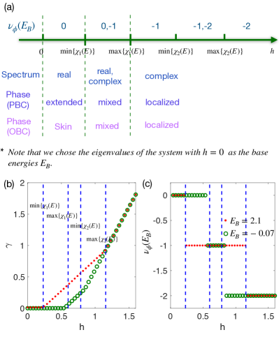
Figure 7: (a)The winding numbers $\nu_{\phi}$, spectrum and phases for the system with potential (26) and $g=0$ v.s. $h$, which is associated with the minimum and maximum values of $\chi_{1,2}(E)$. Numerical results for the LE (b) and the winding numbers $\nu_{\phi}$ (c) of systems with $\lambda_{1}=0.2$, $\lambda_{2}=0.25$, $g=0$ and $E_{B}=-0.071$ and $2.1$ v.s. $h$. For this case, the minimum and maximum values of $\chi_{1,2}(E)$ are $\min\{\chi_{1}(E)\}=0.23$, $\max\{\chi_{1}(E)\}=0.6$, $\min\{\chi_{2}(E)\}=0.786$, and $\max\{\chi_{2}(E)\}=1.156$, respectively.

Next we turn to the Soukoulis-Economou model (26). Take the eigenvalue $E_{B}$ of Hermitian system as the base energy, substitute Eq. (32) into Eq. (39), then one obtains its winding number when changing the parameter $h$:

$$\nu_{\phi}(E_{B},h)=\left\{\begin{array}[]{cc}0,&~{}0<h<\chi_{1}(E_{B}),\\ -1,&~{}\chi_{1}(E)<h<\chi_{2}(E_{B}),\\ -2,&~{}h>\chi_{2}(E_{B}).\\ \end{array}\right.$$ (45)

In Fig. 7 (a), we schematically display the winding number versus the change of $h$. Clearly, the value of winding number depends on the choice of base energy. Fig. 7 (b) and (c) show the numerical results of the LE and winding number as a function of $h$ with $g=0$, $\lambda_{1}=0.2$, $\lambda_{2}=0.25$, $E_{B}=2.1$ and $-0.07$, respectively. When $h=0$, all eigenstates of the system are extended, thus $\gamma(E_{B},0)=0$. It is clear that each of the LE $\gamma(E_{B},h)$ is a continuous piecewise linear function with variable $h$ and has two extreme points $h=\chi_{1}(E_{B})$ and $h=\chi_{2}(E_{B})$, where $\chi_{1,2}(E_{B})$ are the LEs of the dual model (27), as shown in Fig 3 (a). It is obvious that the slope of the LE is zero in the region $0<h<\chi_{1}(E_{B})$ and the winding number $\nu_{\phi}(E_{B},h)=0$, all the eigenstates are extended and all the eigenenergies are real in this region. The slope of the LE $\gamma(E_{B},h)$ is $1$ and the winding number $\nu_{\phi}(E_{B},h)=-1$ in the region $\chi_{1}(E)<h<\chi_{2}(E)$. The slope of the LE $\gamma(E_{B},h)$ is $2$ and the winding number $\nu_{\phi}(E_{B},h)=-2$ if $h>\chi_{2}(E)$. Consequently, according to $\min\{\chi_{1,2}(E_{B})\}$ and $\max\{\chi_{1,2}(E_{B})\}$, the parameter space $h>0$ can be divided into five regions, as shown in Fig.7 (a). In the regions $0<h<\min\{\chi_{1}(E_{B})\}$, $\max\{\chi_{1}(E_{B})\}<h<\min\{\chi_{2}(E_{B})\}$, and $\max\{\chi_{2}(E_{B})\}<h$, the winding numbers $\nu_{\phi}(E_{B},h)$ are $0$, $1$, and $2$, respectively and don’t change with $E_{B}$. In the region $\min\{\chi_{1}(E_{B})\}<h<\max\{\chi_{1}(E_{B})\}$, $\nu_{\phi}(E_{B})=-1$ or $0$, which depends on the selection of $E_{B}$, as shown in Fig.8 (c). Indeed, not only the winding numbers, but also the states are mixed in this region. In the region $\min\{\chi_{2}(E_{B})\}<h<\max\{\chi_{2}(E_{B})\}$, $\nu_{\phi}(E_{B},h)=-2$ or $-1$, which also depends on the the selection of $E_{B}$. Although the winding numbers are mixed, the states are not mixed, all the eigenstates are localized in this region.

IV Robust spectrum and skin effect

In Section II, we unveiled that for general non-Hermitian quasiperiodic models (1), if all the eigenstates of the Hermitian case ($h=0$) are extended, then the real spectrum keeps invariant in the whole extended region $h<\min\{\chi_{1}(E)\}$, i.e. the existence of robust spectrum. In this section, we will show that this kind of intriguing phenomenon could also happen for the non-reciprocal hopping. We will demonstrate this with AA model.

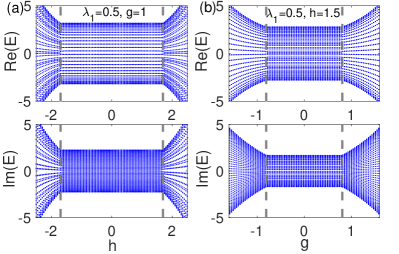
Figure 8: (a) The real and the imaginary part of the eigenvalue spectra versus $h$ for the AA model with $\lambda_{1}=0.5$, $g=1$ and $N=55$. (b) The real and imaginary part of the eigenvalue spectra versus $g$ for the system with $\lambda_{1}=0.5$, $h=1.5$ and $N=55$. Dashed gray lines represent transition points.

For the AA model, and the $\mathcal{PT}$-symmetrical case with $g=0$, the robust spectrum takes place in the regime $|h|<|h_{c}|=-\ln|\lambda_{1}|$. On the other hand, for the case $h=0$, we find that robust spectrum also occurs in the whole localized region $|g|<|g_{c}|=\ln|\lambda_{1}|$. The spectrum properties in these two limits can be understood from the observation that the two limit cases can be related together by a dual transformation jiang2019interplay . For the general case with $g\neq 0$ and $h\neq 0$, with the PBC, the spectrum is complex. Nevertheless, we find that the complex spectrum still keeps invariant when we change $h$ in the extended region $|h|<|h_{c}|=|g|-\ln|\lambda_{1}|$ for a fixed $g$ or change $g$ in the localized region $|g|<|g_{c}|=|h|+\ln|\lambda_{1}|$ for a fixed $h$. To give some concrete examples, we display the spectrum for the system with $\lambda_{1}=0.5$ and $g=1$ versus $h$ in Fig.8(a) and the system with $\lambda_{1}=0.5$ and $h=1.5$ versus $g$ in Fig.8(b). For the case of Fig.8(a), all eigenstates in the region of $|h|<1.7$ are extended state, and the corresponding spectrum does not change with $h$ as long as $|h|<1.7$. For Fig.8(b), all eigenstates in the region of $|g|<0.8$ are localized state, and the corresponding spectrum does not change with $g$ as long as $|g|<0.8$.

Next we shall give a straightforward explanation of robust spectrum shown in Fig.8(b). In the region $|g|<0.8$, the states are localized and are not sensitive to the boundary condition. Therefore, the spectra under PBC and OBC should be the same in the large size limit as long as $|g|<|g_{c}|$. From Eq.(33), we know that the open boundary spectrum is irrelevant with $g$ and should be identical to the case of $g=0$ due to the similar transformation does not change the spectrum. Therefore, it is not hard to understand why the periodic boundary eigenenergies do not change with $g$ for the localized states. When $|g|>|g_{c}|$, the spectra are sensitive to the boundary condition and the corresponding states are extended or skin states under PBC or OBC.

It is not so straightforward to understand the invariance of spectrum shown in Fig.8(a). Nevertheless, we can give an explanation by resorting the dual transformation. From this aspect, it is also useful to consider the ring chain with a flux penetrating through the center, yielding

$$H(\psi) = \sum_{j}(t_{L}e^{i\psi}|j\rangle\langle j+1|+t_{R}e^{-i\psi}|j+1\rangle\langle j|$$ (46)

$$\left.+\lambda_{1}\cos(2\pi\omega j+\theta)|j\rangle\langle j|\right),$$

or equivalently by replacing the hopping term connecting the first and $N$-th site as $h_{IN}=t_{L}e^{-iN\psi}|N\rangle\left\langle 1\right|+t_{R}e^{iN\psi}\left|1\right\rangle\langle N|$, and the winding number is defined as

$$\nu_{\psi}=\frac{1}{2\pi i}\frac{1}{N}\int_{0}^{2\pi}\text{d}\psi\partial_{\psi}\ln\det[H(\psi)-E_{B}].$$ (47)

$\nu_{\psi}$ have been utilized to characterize the loop of the energy spectra of extended and localized states longhiPRL ; jiang2019interplay ; Zeng2020 ; Gong .

By utilizing the dual transformation:

$$\left|j\right\rangle=\frac{1}{\sqrt{N}}\sum_{k}e^{-i2\pi\omega kj}\left|k\right\rangle,$$

we can get a duality form of the Hamiltonian (1) with $\lambda_{l\geqslant 2}=0$, given by

$$\tilde{H}=\sum_{k}\left(\lambda_{L}|k\rangle\left\langle k+1\right|+\lambda_{R}\left|k+1\right\rangle\langle k|+t_{k}|k\rangle\langle k|\right),$$ (48)

where $\lambda_{L}=\lambda_{1}e^{-h}$, $\lambda_{R}=\lambda_{1}e^{h}$ and $t_{k}=2\cos\left(2\pi\omega k+ig\right)$. The Hamiltonian (1) with $\lambda_{l\geqslant 2}=0$ and (48) have similar formulae only with coefficients difference, but have the same spectrum, although the wave functions of two Hamiltonian are entirely different. Let $\lambda_{1}$ as the unit of the energy, we can relabel $g^{\prime}=h$, $h^{\prime}=g$, $\lambda^{\prime}=1/\lambda_{1}$. Now we can see that the case of Fig.8(a) with a fixed $g$ and different $h$ can be mapped to the case with a fixed $h^{\prime}$ and different $g^{\prime}$, i.e., the case of Fig.8(b) in the dual Hamiltonian (48). So we can apply similar explanation why the spectrum is invariant in the region of $g^{\prime}<|g^{\prime}_{c}|$ ($h<|h_{c}|$) for fixed $h^{\prime}$ ($g$). We note under the dual transformation, the flux phase factor $\psi$ is transformed to the phase factor $\phi^{\prime}$ , i.e., $H(\psi,\lambda_{1},h,g)$ is mapping to $\tilde{H}(\phi^{\prime},\lambda^{\prime},h^{\prime},g^{\prime})$. Therefore, from the definitions of Eq.(38) and Eq.(47), we find that $\nu_{\phi,\psi}$ can be related by the following relation

$$\nu_{\psi}(\lambda_{1},h,g)=\nu_{\phi}(1/\lambda_{1},g,h),$$ (49)

i.e., $\nu_{\psi}$ for the system with parameter $\lambda_{1}$, $h$ and $g$ can be obtained from $\nu_{\phi}$ of the corresponding system with $\lambda^{\prime}=1/\lambda_{1}$, $h^{\prime}=g$ and $g^{\prime}=h$.

From the phase diagrams in Figs.4, we always have $\nu_{\phi}=0$ in the extended region and $\nu_{\psi}=\pm 1$. Nonzero winding number $\nu_{\psi}$ indicates the existence of skin states for the system under OBC Yokomizo ; Okuma ; KZhang . On the other hand, we have always $\nu_{\psi}=0$ in the localized region and $\nu_{\phi}=\pm 1$. The relation Eq.(49) constructs a mapping between the phase diagram of $\lambda_{1}<1$ and that of $\lambda_{1}>1$. The winding number $\nu_{\phi}$ ($\nu_{\psi}$) in Fig.4(a) can be read out from $\nu_{\psi}$ ($\nu_{\phi}$) in Fig.4(b) and vice versa.

By comparing the dual Hamiltonian (48) with the original Hamiltonian (1) with $\lambda_{l\geqslant 2}=0$, we can see the existence of a self-duality point at $g=h$ and $\lambda_{1}=1$. At this self-duality point, $\lambda_{c}=1$ is usually taken as the localization-delocalization transition point Zeng2020 . From Eq.(37), we have seen that $\lambda_{c}=1$ is a transition point when $|h|=|g|$, i.e., the self-duality relation is only a special case of our general result Eq.(37). It is worth indicating that our analytical result Eq.(37) does not rely on the self-duality relation or even the dual transformation.

Next we compare the spectra of the system under PBC and OBC to see the sensitivity of spectra to the change of boundary conditions. If non-Hermitian skin effect exists, the system shall display remarkably different eigenspectra under PBC and OBC Okuma ; KZhang ; Lee ; Yokomizo ; Slager . In the Fig.9(a)-(c), we show the spectra in the complex space spanned by Re$(E)$ and Im$(E)$ for systems with $\lambda_{1}=0.5$, $h=1.5$ and $g=-1$, $0.5$ and $1$, respectively, under both PBC and OBC. As shown in Fig.9(b), in the localized region the spectrum under PBC and OBC are almost the same except for several isolated points corresponding to edge states. On the other hand, the spectra under PBC and OBC are obviously different in the delocalized region as shown in Fig.9(a) and 9(c), which is a signature for the existence of skin effect under OBC as witnessed in the distributions of eigenstates shown in Fig.9(d) and 9(f), respectively. The distributions of localized states under PBC and OBC are identical as shown in Fig.9(e), showing clearly that the localized states are independent of the boundary conditions. The numerical results also indicate that the distributions of localized states can be well described by Eq.(34).

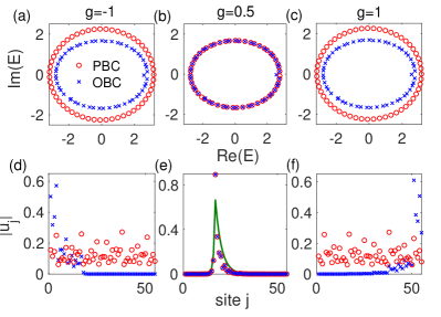
Figure 9: (a)-(c) The complex spectrum for systems with $\lambda_{1}=0.5$, $h=1.5$, $N=55$ and $g=-1$, $0.5$ and $1$, respectively. The red circles and blue crosses represent the eigenvalues under PBC and OBC, respectively. (d)-(f) The distribution of eigenstates corresponding to the minimum real part of eigenvalues for systems with $\lambda_{1}=0.5$, $h=1.5$, $g=-1$, $0.5$ and $1$, respectively. The solid line in (e) is plotted by using Eq.(34).

V Application to other models

V.1 Generalized Ganeshan-Pixley-Das Sarma model

Next we consider the generalized complex Ganeshan-Pixley-Das Sarma model ganeshan2015nearest

$$V_{j}=2\lambda\frac{\cos(2\pi\omega j+ih)}{1-b\cos(2\pi\omega j+ih)},$$ (50)

which is the first quasiperiodic model that the mobility edges have analytic formula for the Hermitian case$(g,h=0)$. By applying Avila’s global theory, the LE of the non-Hermitian model can be easily derived, and the expression is

$$\gamma(E,h)\geq\max\{|h|+\ln\frac{|bE+2\lambda|+\sqrt{(bE+2\lambda)^{2}-4b^{2}}}{2(1+\sqrt{1-b^{2}})},0\},$$ (51)

when $|h|<\ln|\frac{1+\sqrt{1-b^{2}}}{b}|$. The slope of $\gamma(E,h)$ might be $\pm 1$ or $0$. Fig.10 (a) shows the spectrum for the system with $g=0$, $\lambda=0.5$ and $b=0.1$ versus $h$. The spectrum does not change with $h$ in the extended-state region: $h<0.5$. This indicates clearly the existence of robust spectrum in the complex Ganeshan-Pixley-Das Sarma model. For $h>0.5$, the eigenstates with high real part of energies become localized firstly, thus the LE of eigenstates corresponding to the minimum and maximum real part of eigenvalues can determine the mobility edge region, as shown in Fig.10 (b). In the region $h>0.95$, all eigenstates are localized. Then we consider the system with $g\neq 0$. The wavefunction (34) and the transition point (35) tell us that $|g|<\gamma$, the states keep localized, while $|g|>\gamma$, the states become extended, where $\gamma$ is the LE with $g=0$. Fig.10 (c) shows the distribution of eigenstates corresponding to the minimum and maximum real part of eigenvalues for systems with $h=1.2$. Eigenstates are localized with $g=0.1$ and are extended with $g=0.8$, as shown in Fig.10 (c).

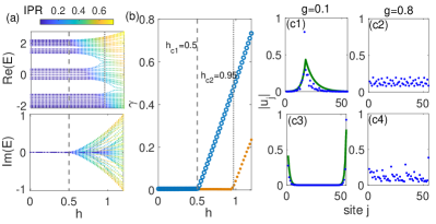
Figure 10: (a) The real and the imaginary part of the eigenvalue spectra versus $h$ for the system with potential (50). Here $g=0$, $\lambda=0.5$, $b=0.1$ and $N=55$. (b)The LE of eigenstates corresponding to the minimum (circles) and maximum(dots) real part of eigenvalues. For accuracy of LE, we choose $N=1597$. (c1) and (c2) The distribution of eigenstates corresponding to the minimum real part of eigenvalues for systems with $\lambda=0.5$, $h=1.2$, $g=0.1$ and $0.8$, respectively. (c3)(c4) The distribution of eigenstates corresponding to the maxmum real part of eigenvalues for systems with $\lambda=0.5$, $h=1.2$, $b=0.1$, $g=0.1$ and $0.8$, respectively. The solid lines in (c1) and (c3) are plotted by using Eq.(34). In (c), $N=55$.

V.2 Quasiperiodic exponential potential

The non-reciprocal hopping model with the quasiperiodic exponential potential

$$V_{j}=Ve^{i(2\pi\omega j+\phi)},$$ (52)

has the same basic idea to determine the transition point (35). The LE of the localized states for this model with $g=0$ is $\gamma=\ln(V)$, so the boundary of localization transition is given by

$$|V|=e^{\left|g\right|}.$$ (53)

The full details for the calculation of the LE are given in Appendix. While all eigenstates are localized for $|V|>e^{\left|g\right|}$, the eigenstates are extended states (skin states) under PBC (OBC) for $|V|<e^{\left|g\right|}$. When $g=0$, the model reduces to the one studied in Ref.longhi2019metal and no skin effect occurs. For $g\neq 0$, skin effect occurs in the region of $|V|<e^{\left|g\right|}$.

The unusual spectrum feature can be also found in this model. Eq.(53) suggests that the localized phase exists only for $|V|>1$. For a given $V$ with $|V|>1$, the system is in localized phase in the region $|g|<g_{c}$ with $g_{c}=\ln|V|$. We find that the spectrum of the system is invariant with the change of $g$ as long as $|g|<g_{c}$, which is verified by our numerical result and can be explained in a similar way as given in the above subsection.

VI Summary and outlook

In summary, based on Avila’s global theory, one of his Fields medal work, we developed a rigorous and general scheme for the study of non-Hermitian quasiperiodic systems with both complex phase factor and non-reciprocal hopping. We demonstrated that the localization-delocalization transition point, $\mathcal{PT}$-symmetry-breaking point for general non-Hermitian quasicrystals with $h\neq 0$, can be described by a conclusion expression $h=\min\{\chi_{1}(E)\}$, where $\chi_{1}(E)$ is the smallest positive LE of its dual model with $h=0$ for a given eigenvalue $E$. The general relation between winding numbers and acceleration is also unveiled, consequently we obtained that the winding number is just the slope of LE, and the topological transition points for the winding numbers are determined by all dual-model LEs $h=\chi_{i}(E)$. These results are applied to study the typical examples, including both the non-Hermitian AA model and Soukoulis-Economou model. Especially, for the non-Hermitian AA model, we analytically determined the complete phase diagram in the whole parameter space, which can be alternatively characterized by winding numbers. Moreover, we discovered an intriguing feature of robust spectrum, i.e., the spectrum keeps invariant under the change of the complex phase parameter $h$ or non-reciprocal parameter $g$ as long as $h<|h_{c}|$ or $g<|g_{c}|$ for system in the extended or localized region, respectively. We found that the existence of robust spectrum is a very common feature of non-Hermitian quasiperiodic systems. Models beyond the two typical examples are also discussed. Our analysis open a door to further study intriguing properties of non-Hermitian quasicrystals.

Photonic systems provide a valid platform of realization of non-Hermitian Hamiltonians with quasiperiodic potentials, which are manifested by the gain and loss of the laser pulse inside the optic fiber. Many typical phenomena have been observed in photonic experiments, such as PT symmetry, exceptional points, non-Hermitian skin effect., etc. Regensburger11 ; Regensburger12 ; Wimmer15 ; Vatnik17 ; Derevyanko19 ; Weidemann20 . We expect that our theoretical work shall stimulate the experimental study of localization transition in non-Hermitian quasiperiodic systems.

Appendix A Global theory of one-frequency cocycle

Suppose that $A$ is an analytic function from the circle $S^{1}$ to the group $SL(2,C)$, an analytic quasiperiodic cocycle $(\omega,A)$ can be seen as a linear skew product:

$$(\omega,A):S^{1}\times R^{2}\rightarrow S^{1}\times R^{2}$$

$$(\theta,v)\mapsto(\theta+\omega,A(\theta)\cdot v).$$

If $A(\theta)$ admits a holomorphic extension to $|Im\theta|<\delta$, then for $|\epsilon|<\delta$ we can define $A_{\epsilon}(\theta)=A(\theta+i\epsilon)$, and define its LE by

$$\gamma\left(E,h\right)=\lim_{n\rightarrow\infty}\frac{1}{2\pi n}\int_{0}^{2\pi}\ln\left|\left|T_{n}\left(E,\phi,h\right)\right|\right|d\phi,$$ (54)

where $T_{n}$ is the transfer matrix. The key observation of Avila’s global theory is that $h\rightarrow\gamma\left(E,h\right)$ is convex and piecewise linear, with right-derivatives satisfying

$$\lim_{h\rightarrow 0_{+}}\frac{1}{2\pi h}(\gamma\left(E,h\right)-\gamma\left(E,0\right))\in\mathbb{Z}.$$

Similarly, the left-derivative satisfy

$$\lim_{h\rightarrow 0_{-}}\frac{1}{2\pi h}(\gamma\left(E,h\right)-\gamma\left(E,0\right))\in\mathbb{Z}.$$

Note a sequence $(u_{n})_{n\in\mathbb{Z}}$ is a formal solution of the eigenvalue equation

$$u_{n+1}+u_{n-1}+V(\theta+n\omega)u_{n}=Eu_{n}$$

if and only if it satisfied

$$\begin{pmatrix}u_{n+1}\\ u_{n}\end{pmatrix}=\begin{pmatrix}E-v(\theta+n\omega)&-1\cr 1&0\end{pmatrix}\begin{pmatrix}u_{n}\\ u_{n-1}\end{pmatrix},$$

therefore, any quasiperiodic model (1) can be seen as a quasi-periodic cocycle.

Generally speaking, it is difficult to exactly calculate the LE, however Avila’s global theory actually provide an efficient way to calculate the LE, thus to determine to localize-delocalize transition. In the following, we will illustrate this by two well-known models, and explain the general results:

A.1 AA model

The eigenvalue equation of AA model is

$$u_{n+1}+u_{n-1}+2\lambda_{1}\cos 2\pi(\theta+n\omega)u_{n}=Eu_{n},$$

thus the corresponding cocycle is $(\omega,T(\theta))$ where

$$T(\theta)=\begin{pmatrix}E-2\cos\theta&-1\cr 1&0\end{pmatrix}.$$

Let us complexify the phase, and let $h\rightarrow+\infty$, direct computation shows that

$$T(\phi+ih)=e^{h}e^{i2\pi(\theta+\omega)}\left(\begin{array}[]{cc}-\lambda&0\\ 0&0\\ \end{array}\right)+o(1).$$

Thus we have $\gamma\left(E,h\right)=h+\log|\lambda|+o(1).$ Note $\gamma(E,h)$ is a convex, piecewise linear function of $h$ with their slopes being integers, thus if $h$ is large enough,

$$\gamma\left(E,h\right)=h+\log|\lambda|.$$

Furthermore, $E$ does not lie in the spectrum of the Hamiltonian $H$, if and only if $\gamma(E,h)>0$, and $\gamma(E,h)$ is a linear functions around $h$. Thus if the energy $E$ lies in the spectrum, we have

$$\gamma\left(E,h\right)=\max\{\ln|\lambda|+h,0\},\forall h\geq 0.$$

Note $T(\theta)\in SL(2,\mathbb{R})$, thus the LE is an even function with respect to $h$, which gives

$$\gamma\left(E,h\right)=\max\{\ln|\lambda|+|h|,0\},\forall h\in\mathbb{R}.$$

A.2 Complex quasiperiodic potential

For the complex quasiperiodic model $V_{n}=Ve^{-i(2\pi\omega n+\phi)},$ the transfer matrix takes the form

$$T(\phi)=\left(\begin{array}[]{cc}E-Ve^{i(2\pi\omega+\phi)}&-1\\ 1&0\\ \end{array}\right),$$

thus $T(\phi)\in SL(2,\mathbb{C})$, not belongs to $SL(2,\mathbb{R})$ anymore, thus compared to the AA model, the LE is not an even function with respect to $h$. Still if we complexify the phase, and let $h\rightarrow+\infty$, direct computation shows that

$$T(\phi+ih)=e^{h}e^{-i2\pi(\phi+\omega)}\left(\begin{array}[]{cc}-V&0\\ 0&0\\ \end{array}\right)+o(1).$$

Thus we have $\gamma\left(E,h\right)=h+\log|V|+o(1),h\geq 0$. Note $\gamma(E,h)$ is a convex, piecewise linear function of $h$ with their slopes being integers, then if the energy belongs to the spectrum, then

$$\gamma\left(E,h\right)=\max\{\ln|\lambda|+h,0\},\forall h\geq 0,$$

consequently, we have

$$\gamma\left(E,0\right)=\max\{\ln|V|,0\}.$$

On the other hand, for the model $V_{n}=Ve^{i(2\pi\omega n+\phi)},$ we can omplexify the phase, and let $h\rightarrow-\infty$, which gives us $\gamma\left(E,h\right)=-h+\log|V|+o(1),h\leq 0$. Similarly, we have

$$\gamma\left(E,0\right)=\max\{\ln|V|,0\}.$$ (55)

A.3 General models

As we mentioned above, one of the fundamental results of Avila’s global theory is that $\gamma\left(E,h\right)$ is a piecewise affine function in $h$ for each $E$, and the slope of each piece is an integer. Indeed, as proved in GJYZ , one can give the exact turning points of $\gamma\left(E,h\right)$ and the exact slope of it in every piece, which can be seen as quantitative version of Avila’s global theory, in the following, we will try to explain this:

For any trigonometric polynomials

$$V_{j}=\sum_{k=1}2\lambda_{l}\cos(2l\pi\omega j),$$

consider the quasi-periodic model

$$Eu_{j}=u_{j+1}+u_{j-1}+V_{j}u_{j},\ \ j\in\mathbb{Z}.$$ (56)

Through the transformation

$$u_{j}=\sum_{k}e^{i2\pi\omega kj}\tilde{u}_{k},\ \ k\in\mathbb{Z},$$

the dual model has the form

$$E\tilde{u}_{k}=\sum\limits_{l=-d}^{d}\lambda_{|l|}\tilde{u}_{k+l}+2\cos(2\pi\omega k)\tilde{u}_{k}.$$ (57)

The model (57) can be written as the following form

$$\tilde{u}_{k+d}=\frac{1}{\lambda_{d}}\big{\{}\left[E-2\cos(2\pi\omega k)\right]\tilde{u}_{k}-\sum\limits_{l=-d}^{d-1}\lambda_{|l|}\tilde{u}_{k+l}\big{\}}.$$ (58)

So the matrix form for the model (58) can be written as

$$\left(\begin{array}[]{c}\tilde{u}_{k+d}\\ \vdots\\ \tilde{u}_{k+1}\\ \tilde{u}_{k}\\ \vdots\\ \tilde{u}_{k-d+1}\\ \end{array}\right)=A^{k}\left(\begin{array}[]{c}\tilde{u}_{k+d-1}\\ \vdots\\ \tilde{u}_{k}\\ \tilde{u}_{k-1}\\ \vdots\\ \tilde{u}_{k-d}\\ \end{array}\right),$$

where

$$A^{k}=\left(\begin{array}[]{cccccc}\frac{-\lambda_{d-1}}{\lambda_{d}}&\cdots&\frac{E-2\cos(2\pi\omega k)}{\lambda_{d}}&\frac{-\lambda_{1}}{\lambda_{d}}&\cdots&-1\\ 1&\cdots&0&0&\cdots&0\\ 0&\ddots&&&&0\\ \vdots&&1&&&\vdots\\ &&&\ddots&&\\ 0&\cdots&&&1&0\\ \end{array}\right)$$

is a $2d\times 2d$ matrix. Then we can define the matrix

$$\mathbf{\Theta}=\left(T_{N}^{{\dagger}}T_{N}\right)^{1/(2N)},$$ (59)

where $T_{N}=\prod_{k}A^{k}$ is the total transfer matrix. When $N\rightarrow\infty$, $\mathbf{\Theta}$ is finite, which can be guaranteed by Oseledec’s ergodic theorem. The LEs are

$$\chi_{i}=\ln\theta_{i},$$

where $\theta_{i}$ are the eigenvalues of matrix $\mathbf{\Theta}$.

It is easy to check that

$$T^{dn}=\prod_{k=dn}^{dn+d-1}A^{k}=\left(\begin{array}[]{cc}C_{d}^{-1}(EI-B_{dn})&-C_{d}^{-1}C_{d}^{*}\\ I_{d}&O_{d}\\ \end{array}\right),$$ (60)

where

$$C_{d}=\left(\begin{array}[]{ccc}\lambda_{d}&\ldots&\lambda_{1}\\ 0&\ddots&\vdots\\ 0&0&\lambda_{d}\\ \end{array}\right),$$

$C_{d}^{*}$ is its adjoint and $B_{dn}$ is the Hermitian matrix

$$B_{dn}=\left(\begin{array}[]{cccc}W_{dn+n-1}&\lambda_{1}&\ldots&\lambda_{d-1}\\ \lambda_{1}&\ddots&\ddots&\vdots\\ \vdots&\ddots&W_{dn+1}&\lambda_{1}\\ \lambda_{d-1}&\ldots&\lambda_{1}&W_{dn}\\ \end{array}\right),$$

where $W_{k}=2\cos(2\pi\omega k)$, $I_{d}$ and $O_{d}$ are the $d$-dimensional identity and zero matrices.

Note the matrix (60) is complex symplectic, thus the eigenvalues of (59) will come in pairs, then the LEs can be denoted by $\pm\chi_{1},\cdots,\pm\chi_{\ell}$ with multiplicity $n_{1},\cdots,n_{\ell}$ respectively. We may assume that $0\leq\chi_{1}(E)<\cdots<\chi_{\ell}(E)$. It is obvious that $n_{1}+\cdots+n_{\ell}=d$.

As proved in GJYZ , the LEs for the model (1) with $g=0$ can be written as the following:

$$\gamma\left(E,h\right)=\left\{\begin{array}[]{cc}\gamma(E,0),&~{}~{}h\in[0,\chi_{1}(E)],\\ \vdots&\vdots\\ \gamma(E,\chi_{i}(E))+(h-\chi_{i}(E))\sum_{j=1}^{i}{n_{j}},&~{}~{}h\in(\chi_{i}(E),\chi_{i+1}(E)],\\ \vdots&\vdots\\ \gamma(E,\chi_{\ell}(E))+(h-\chi_{l}(E))\sum_{j=1}^{\ell}{n_{j}},&~{}~{}h\in(\chi_{\ell}(E),\infty),\end{array}\right.$$ (66)

where $E\in\mathbb{C}$ and $1<i<\ell$. For the $\mathcal{PT}$-symmetrical case: the model (1) with $g=0$, the boundaries of the extended-mixed transformation and mixed-localized transformation can be determined by $h=\min(\chi_{1}(E))$ and $h=\max(\chi_{1}(E))$, which only depends on $\chi_{1}(E)$ in connection with longest localization length for the dual model (58).

Appendix B Winding number $\nu_{\phi}$ for $g=0$ and $g\neq 0$

The definition of winding number $\nu_{\phi}$ is

$$\nu_{\phi}(g) = \lim_{N\rightarrow\infty}\frac{1}{2\pi i}\int_{0}^{2\pi}\text{d}\phi\partial_{\phi}\frac{\ln\det[H(\theta,g)-E_{B}]}{N}$$ (67)

$$= \lim_{N\rightarrow\infty}\frac{1}{2\pi i}\int_{0}^{2\pi}\text{d}\phi\partial_{\phi}\zeta(E_{B},\theta,g),$$

where $\theta=\phi+ih$ and the analytical function

$$\zeta(E_{B},\theta,g)=\frac{\ln D_{n}(E_{B},\theta,g)}{N}.$$ (68)

with

$$D_{n}(E_{B},\theta,g)=\det|H(\theta,g)-E_{B}|.$$

According to the Cauchy-Riemann equation in complex form, we can get

$$\frac{\partial\zeta(E_{B},\theta,g)}{\partial h}=i\frac{\partial\zeta(E_{B},\theta,g)}{\partial\phi}.$$ (69)

Then we can get

$$\nu_{\phi} = \frac{1}{2\pi i}\lim_{N\rightarrow\infty}\int_{0}^{2\pi}\text{d}\phi\partial_{\phi}\zeta(E_{B},\theta,g)$$

$$= -\frac{1}{2\pi}\lim_{N\rightarrow\infty}\int_{0}^{2\pi}\text{d}\phi\partial_{h}\zeta(E_{B},\theta,g)$$

$$= -\frac{1}{2\pi}\lim_{N\rightarrow\infty}\partial_{h}\int_{0}^{2\pi}\text{d}\phi\zeta(E_{B},\theta,g).$$

When $g=0$ and $n\rightarrow\infty$, the normal of the transfer matrix is

$$\lim_{n\rightarrow\infty}\frac{\ln||T_{n}(E_{B},\theta)||}{N}=\lim_{n\rightarrow\infty}\zeta(E_{B},\theta,0).$$

The transfer matrix of the system with $g=0$ can be written as

$$T_{n}\left(E,\theta\right)=\prod_{j=1}^{n}T^{j}=\prod_{j=1}^{n}\left(\begin{array}[]{cc}E-V_{j}&-1\\ 1&0\end{array}\right).$$

The transfer matrix can also be expressed

$$T_{n}\left(E,\theta\right)=\left(\begin{array}[]{cc}D_{n}(E_{B},\theta,0)&-D_{n-1}(E_{B},\theta,0)\\ D_{n-1}(E_{B},\theta,0)&-D_{n-2}(E_{B},\theta,0).\end{array}\right).$$

Then we can get

$$\lim_{N\rightarrow\infty}\int_{0}^{2\pi}\text{d}\phi\zeta(E_{B},\theta,0)$$

$$= \lim_{N\rightarrow\infty}\int_{0}^{2\pi}\text{d}\phi\frac{\ln||T_{N}(E_{B},\theta)||}{N}$$

$$= 2\pi\gamma(E_{B},h).$$

Finally we get the relaiton

$$\nu_{\phi}(0)=-\partial_{h}\gamma(E_{B},h).$$

Now, we calculate the winding number of system with $g\neq 0$. The Hamiltonian with a general boundary condition in matrix form can be written as

$$H\left(\phi,g\right)=\left(\begin{array}[]{ccccc}V_{1}&1&&&\eta e^{Ng}\\ 1&V_{2}&1&&\\ &\ddots&\ddots&\ddots&\\ &&1&V_{N-1}&1\\ \eta e^{-Ng}&&&1&V_{N}\\ \end{array}\right).$$ (70)

where $\eta$ is a finite value. $\eta=0$ or $1$ is corresponding to PBC or OBC. In the large $N$ limit, the determinant of $H\left(\phi\right)$ is

$$\det H\left(\phi,g\right)$$

$$= (-1)^{N+1}\eta e^{N|g|}-2\times(-1)^{N+1}+\det H\left(\phi,0\right).$$

First we calculate the integrand

$$\frac{1}{2\pi i}\partial_{\phi}\frac{\ln[D(E_{B},\theta,g)]}{N}=\frac{1}{2\pi i}\frac{\partial_{\phi}D(E_{B},\theta,0)}{ND(E_{B},\theta,g)}$$

$$= \frac{1}{2\pi i}\frac{\partial_{\phi}D(E_{B},\theta,0)}{N((-1)^{N+1}\eta e^{Ng}+D(E_{B},\theta,0))}.$$

To calculate the above equation, we need to get the behavior of $\partial_{\phi}D(E_{B},\theta,0)$ and $D(E_{B},\theta,0)$. According to the definition of the LE,

$$\lim_{N\rightarrow\infty}\ln|D(E_{B},\theta,0)|/N=\gamma$$ (71)

and thus $|D(E_{B},\theta,0)|$ can be written as

$$|D(E_{B},\theta,0)|=e^{\gamma N}.$$

According to the definition of the winding number,

$$\lim_{N\rightarrow\infty}\frac{1}{2\pi i}\int_{0}^{2\pi}\text{d}\phi\partial_{\phi}\frac{\ln\det[H(\theta,0)-E_{B}]}{N}=\nu_{\phi}(0),$$

we can get

$$\frac{\partial_{\phi}D(E_{B},\theta,0)}{D(E_{B},\theta,0)}=N\Omega(\psi),$$

with

$$\lim_{N\rightarrow\infty}\int_{0}^{2\pi}\Omega(\psi)=2\pi\nu_{\phi}(0)i.$$

Then, we can get

$$\frac{1}{2\pi i}\partial_{\phi}\frac{\ln[D(E_{B},\theta,g)]}{N}$$ (74)

$$= \left\{\begin{array}[]{cc}0,&|g|>\gamma\\ \Omega(\psi),&|g|<\gamma\end{array}\right.,$$

for $\eta\neq 0$ and

$$\frac{1}{2\pi i}\partial_{\phi}\frac{\ln[D(E_{B},\theta,g)]}{N}=\Omega(\psi),$$ (75)

for $\eta=0$. Finally, substitution of Eq. (74) into Eq. (67) gets the winding number of system with $g\neq 0$ and $\eta\neq 0$

$$\nu_{\phi}(g)= \lim_{N\rightarrow\infty}\frac{1}{2\pi i}\int_{0}^{2\pi}\text{d}\phi\partial_{\phi}\frac{\ln\det[H(\theta,g)-E_{B}]}{N}$$

$$= \left\{\begin{array}[]{cc}0,&|g|>\gamma\\ \nu_{\phi}(0)=-\partial_{h}\gamma(E_{B},h),&|g|<\gamma.\end{array}\right.$$ (78)

Substitution of Eq. (75) into Eq. (67) get the winding number of system under OBC ($\eta=0$)

$$\nu_{\phi}(g)=\nu_{\phi}(0).$$ (79)

Thus we can get that the winding number remains unchanged under the different boundary conditions except OBC.

References

- (1) P. W. Anderson, Absence of diffusion in certain random lattices, Phys. Rev. 109, 1492(1958).
- (2) E. Abrahams, P. W. Anderson, D. C. Licciardello, and T. V. Ramakrishnan, Scaling theory of localization: Absence of quantum diffusion in two dimensions, Phys. Rev. Lett. 42, 673 (1979).
- (3) D J Thouless, A relation between the density of states and range of localization for one dimensional random systems, J. Phys. C: Solid State Phys. 5, 77 (1972).
- (4) P. A. Lee and T. V. Ramakrishnan, Disordered electronic systems, Rev. Mod. Phys. 57, 287(1985).
- (5) F. Evers and A. D. Mirlin, Anderson transitions, Rev. Mod. Phys. 80, 1355 (2008).
- (6) G. Roati, C. DErrico, L. Fallani, M. Fattori, C. Fort, M. Zaccanti, G. Modugno, M. Modugno, and M. Inguscio, Anderson localization of a non-interacting bose Ceinstein condensate, Nature (London) 453, 895 (2008).
- (7) H. P. Lüschen, S. Scherg, T. Kohlert, M. Schreiber, P. Bordia, X. Li, S. Das Sarma, and I. Bloch, Single-particle mobility edge in a one-dimensional quasiperiodic optical lattice, Phys. Rev. Lett. 120, 160404 (2018).
- (8) S. Aubry and G. André, Analyticity breaking and Anderson localization in incommensurate lattices, Ann. Israel Phys. Soc. 3, 133 (1980).
- (9) D. J. Thouless, Localization by a potential with slowly varying period, Phys. Rev. Lett. 61, 2141(1988).
- (10) M. Kohmoto, Metal-insulator transition and scaling for incommensurate systems, Phys. Rev. Lett. 26, 1198 (1983).
- (11) S. Y. Jitomirskaya, Metal-insulator transition for the almost mathieu operator, Ann. Math. 3, 150 (1999).
- (12) H. A. Ceccatto, Quasiperiodic Ising Model in a Transverse Field: Analytical Results, Phys. Rev. Lett. 62, 203 (1989).
- (13) L. Zhou, H. Pu, and W. Zhang, Anderson localization of cold atomic gases with effective spin-orbit interaction in a quasiperiodic optical lattice, Phys. Rev. A 87, 023625 (2013).
- (14) M. Kohmoto and D. Tobe, Localization problem in a quasiperiodic system with spin-orbit interaction, Phys. Rev. B 77, 134204 (2008).
- (15) X. Cai, L.-J. Lang, S. Chen, and Y. Wang, Topological superconductor to Anderson localization transition in one-Dimensional incommensurate lattices, Phys. Rev. Lett. 110, 176403 (2013).
- (16) W. DeGottardi, D. Sen, and S. Vishveshwara, Majorana fermions in superconducting 1D systems having periodic, quasiperiodic, and disordered Potentials, Phys. Rev. Lett. 110, 146404 (2013).
- (17) F. Liu, S. Ghosh, and Y. D. Chong, Localization and Adiabatic Pumping in a Generalized Aubry-Andre-Harper Model, Phys. Rev. B 91, 014108 (2015).
- (18) A. Chandran and C. R. Laumann, Localization and Symmetry Breaking in the Quantum Quasiperiodic Ising Glass, Phys. Rev. X 7, 031061 (2017).
- (19) Y.-C. Wang, X.-J. Liu and S. Chen. Properties and applications of one dimensional quasiperiodic lattices. Acta Physica Sinica, 68 040301, (2019).
- (20) J. Biddle, D. J. Priour, B. Wang, and S. Das Sarma, Localization in one-dimensional lattices with non-nearest-neighbor hopping: Generalized Anderson and Aubry- André models, Phys. Rev. B 83, 075105 (2011).
- (21) J. Biddle and S. Das Sarma, Predicted mobility edges in one-dimensional incommensurate optical lattices: An exactly solvable model of Anderson localization, Phys. Rev. Lett. 104, 070601 (2010).
- (22) S. Ganeshan, J. H. Pixley, and S. Das Sarma, Nearest neighbor tight binding models with an exact mobility edge in one dimension, Phys. Rev. Lett. 114, 146601 (2015).
- (23) X. P. Li, J. H. Pixley, D. L. Deng, S. Ganeshan, and S. Das Sarma, Quantum nonergodicity and fermion localization in a system with a single-particle mobility edge, Phys. Rev. B 93, 184204 (2016).
- (24) X. Li, X. P. Li, and S. Das Sarma, Mobility edges in one-dimensional bichromatic incommensurate potentials, Phys. Rev. B 96, 085119 (2017).
- (25) X. Li and S. Das Sarma, Mobility edge and interme-diate phase in one-dimensional incommensurate lattice potentials, Phys. Rev. B 101, 064203 (2020).
- (26) X. Deng, S. Ray, S. Sinha, G. V. Shlyapnikov, and L. Santos, One-Dimensional Quasicrystals with Power-Law Hopping, Phys. Rev. Lett. 123, 025301 (2019).
- (27) S. Das Sarma, S. He, and X. C. Xie, Mobility edge in a model one-dimensional potential, Phys. Rev. Lett. 61, 2144 (1988).
- (28) S. Das Sarma, S. He, and X. C. Xie, Localization, mobility edges, and metal-insulator transition in a class of one-dimensional slowly varying deterministic potentials, Phys. Rev. B 41, 5544 (1990).
- (29) Y. Wang, X. Xia, L. Zhang, H. Yao, S. Chen, J. You, Q. Zhou, and X. Liu, One dimensional quasiperiodic mosaic lattice with exact mobility edges, Phys. Rev. Lett. 125, 196604 (2020).
- (30) D. Bernard and A. LeClair, A classification of non-Hermitian random matrices, arXiv:0110649.
- (31) K. Kawabata, K. Shiozaki, M. Ueda, and M. Sato, Symmetry and topology in non-Hermitian physics, Phys. Rev. X 9, 041015 (2019).
- (32) H. Zhou and J. Y. Lee, Periodic table for topological bands with non-Hermitian symmetries, Phys. Rev. B 99, 235112 (2019).
- (33) C.-H. Liu, and S. Chen, Topological classification of defects in non-Hermitian systems, Phys. Rev. B 100, 144106 (2019).
- (34) I. Y. Goldsheid and B. A. Khoruzhenko, Distribution of Eigenvalues in Non-Hermitian Anderson Models, Phys. Rev. Lett. 80 2897 (1998).
- (35) L. G. Molinari, Non-Hermitian spectra and Anderson localization, J. Phys. A: Math. Theor. 42 265204 (2009).
- (36) H. Markum, R. Pullirsch, and T. Wettig, Non-Hermitian Random Matrix Theory and Lattice QCD with Chemical Potential Phys. Rev. Lett. 83, 484 (1999).
- (37) J. T. Chalker and B. Mehlig, Eigenvector Statistics in Non-Hermitian Random Matrix Ensembles Phys. Rev. Lett. 81, 3367 (1998).
- (38) R. Hamazaki, K. Kawabata, N. Kura, and M. Ueda, Universality classes of non-hermitian random matrices, Phys. Rev. Research 2, 023286 (2020).
- (39) C. Wang and X. R. Wang, Level statisitcs of extended states in random non-Hermitian Hamiltonians, Phys. Rev. B 101, 165114 (2020).
- (40) X. Luo, T. Ohtsuki, and R. Shindou, Universality Classes of the Anderson Transitions Driven by Non-Hermitian Disorder, Phys. Rev. Lett. 126, 090402 (2021).
- (41) K. kawabata and S. Ryu, Nonunitary scaling theory of non-Hermitian localization, arXiv:2005.00604.
- (42) N. Hatano and D. R. Nelson, Localization transitions in non-hermitian quantum mechanics, Phys. Rev. Lett. 77, 570 (1996).
- (43) N. Hatano and D. R. Nelson, Non-hermitian delocalization and eigenfunctions, Phys. Rev. B 58, 8384 (1998).
- (44) A. V. Kolesnikov and K. B. Efetov, Localization- delocalization transition in non-hermitian disordered systems, Phys. Rev. Lett. 84, 5600 (2000).
- (45) Z. Gong, Y. Ashida, K. Kawabata, K. Takasan, S. Higashikawa, and M. Ueda, Topological Phases of Non-Hermitian Systems, Phys. Rev. X 8, 031079 (2018).
- (46) D.-W. Zhang, L.-Z. Tang, L.-J. Lang, H. Yan, and S.-L. Zhu, Non-hermitian topological anderson insulators, Sci. China Phys. Mech. 63, 1 (2020).
- (47) J. Claes and T. L. Hughes, Skin effect and winding number in disordered non-Hermitian systems, arXiv:2007.03738.
- (48) L.-Z. Tang, L.-F. Zhang, G.-Q. Zhang, and D.-W. Zhang, Topological Anderson insulators in two-dimensional non-Hermitian disordered systems, Phys. Rev. A 101, 063612 (2020).
- (49) Y. Huang and B. I. Shklovskii, Anderson transition in three-dimensional systems with non-Hermitian disorder, Phys. Rev. B 101, 014204 (2020).
- (50) A. F. Tzortzakakis, K. G. Makris, and E. N. Economou, Non-Hermitian disorder in two-dimensional optical lattices, Phys. Rev. B 101, 014202 (2020).
- (51) A. Jazaeri and I. I. Satija, Localization transition in incommensurate non-hermitian systems, Phys. Rev. E 63, 036222 (2001).
- (52) C. Yuce. symmetric Aubry-Andre model, Phys. Lett. A 378, 2024 (2014).
- (53) Q.-B. Zeng, S. Chen, and R. Lu, Anderson localization in the non-Hermitian Aubry-Andre-Harper model with physical gain and loss, Phys. Rev. A 95, 062118 (2017).
- (54) S. Longhi, Metal-insulator phase transition in a non-hermitian aubry-andré-harper model, Phys. Rev. B 100, 125157 (2019).
- (55) S. Longhi, Topological phase transition in non-hermitian quasicrystals, Phys. Rev. Lett. 122, 237601 (2019).
- (56) H. Jiang, L. J. Lang, C. Yang., S. L. Zhu, and S. Chen, Interplay of non-hermitian skin effects and anderson localization in nonreciprocal quasiperiodic lattices, Phys. Rev. B 100, 054301 (2019).
- (57) Q. B. Zeng, Y. B. Yang, and Y. Xu, Topological phases in non-hermitian aubry-andré-harper models, Phys. Rev. B 101, 020201 (2020).
- (58) Y. Liu, X.-P. Jiang, J. Cao, and S. Chen, Non-Hermitian mobility edges in one-dimensional quasicrystals with parity-time symmetry, Phys. Rev. B 101, 174205 (2020).
- (59) Q.-B. Zeng and Y. Xu, Winding numbers and generalized mobility edges in non-Hermitian systems, Phys. Rev. Research 2, 033052 (2020).
- (60) T. Liu, H. Guo, Y. Pu, and S. Longhi, Generalized Aubry-Andre self-duality and mobility edges in non-Hermitian quasiperiodic lattices Phys. Rev. B 102, 024205 (2020).
- (61) Y. Liu, Y. Wang, X.-J. Liu, Q. Zhou, and S. Chen, Exact mobility edges, PT-symmetry breaking and skin effect in one-dimensional non-Hermitian quasicrystals, Phys. Rev. B 103, 014203 (2021).
- (62) X. Cai, Boundary-dependent Self-dualities, Winding Numbers and Asymmetrical Localization in non-Hermitian Quasicrystals, Phys. Rev. B 103, 014201 (2021).
- (63) S. Longhi, Phase transitions in a non-Hermitian Aubry-André-Harper model, Phys. Rev. B 103, 054203 (2021).
- (64) L.-J. Zhai, S. Yin, G.-Y. Huang, Many-body localization in a non-Hermitian quasi-periodic system, Phys. Rev. B 102, 064206 (2020).
- (65) Y. Liu, Y. Wang, Z. Zheng, S. Chen, Exact non-Hermitian mobility edges in one-dimensional quasicrystal lattice with exponentially decaying hopping and its dual lattice, Phys. Rev. B 103, 134208 (2021).
- (66) L.-Z. Tang, G.-Q. Zhang, L.-F. Zhang, D.-W. Zhang, Localization and topological transitions in non-Hermitian quasiperiodic lattices, arXiv:2101.05505.
- (67) X. Cai, Anderson localization and topological phase transitions in non-Hermitian Aubry-Andre-Harper models with p-wave pairing, arXiv:2103.04107.
- (68) A. Avila, Global theory of one-frequency Schröinger operators, Acta. Math. 1, 215, (2015).
- (69) A. Avila, J. You , Q. Zhou, Sharp phase transitions for the almost Mathieu operator, Duke. Math. J. 14, 166 (2017)
- (70) C. M. Bender and S. Boettcher, Real spectra in non-hermitian hamiltonians having PT symmetry. Phys. Rev. Lett. 80, 5243 (1998).
- (71) L. Ge, S. Y. Jitomirskaya, J. You and Q. Zhou. Quantitative global theory of one-frequency quasiperiodic operators. Preprint
- (72) A. Avila, S. Y. Jitomirskaya, The Ten Martini Problem. Ann. of Math, 170, 303-342 (2009).
- (73) C. M. Soukoulis and E. N. Economou, Localization in One-Dimensional Lattices in the Presence of Incommensurate Potentials. Phys. Rev. Lett. 48, 1043 (1982).
- (74) S. Yao and Z. Wang, Edge states and topological invariants of non-Hermitian systems, Phys. Rev. Lett. 121, 086803 (2018).
- (75) Y. Xiong, Why does bulk boundary correspondence fail in some non-Hermitian topological models, J. Phys. Commun. 2, 035043 (2018).
- (76) V. M. Martinez Alvarez, J. E. Barrios Vargas, and L. E. F. Foa Torres, Non-Hermitian robust edge states in one dimension: Anomalous localization and eigenspace condensation at exceptional points, Phys. Rev. B 97, 121401(R) (2018).
- (77) F. K. Kunst, E. Edvardsson, J. C. Budich, and E. J. Bergholtz, Biorthogonal, bulk-boundary correspondence in non-Hermitian systems, Phys. Rev. Lett. 121, 026808 (2018).
- (78) C. H. Lee and R. Thomale, Anatomy of skin modes and topology in non-Hermitian systems, Phys. Rev. B 99, 201103(R) (2019).
- (79) K. Yokomizo and S. Murakami, Non-Bloch band theory of non-Hermitian system, Phys. Rev. Lett. 123, 066404 (2019).
- (80) K. Zhang, Z. Yang, and C. Fang, Correspondence between winding numbers and skin modes in non-hermitian systems, Phys. Rev. Lett. 125, 126402 (2020).
- (81) N. Okuma, K. Kawabata, K. Shiozaki, and M. Sato, Topological Origin of Non-Hermitian Skin Effects, Phys. Rev. Lett. 124, 086801 (2020).
- (82) D. S. Borgnia, A. J. Kruchkov, R.-J. Slager, Non-Hermitian Boundary Modes, Phys. Rev. Lett. 124, 056802 (2020).
- (83) A. Regensburger, C. Bersch, B. Hinrichs, G. Onishchukov, A. Schreiber, C. Silberhorn, and U. Peschel, Photon Propagation In A Discrete Fiber Network: An Interplay Of Coherence And Losses, Phys. Rev. Lett. 107, 233902 (2011).
- (84) A. Regensburger, C. Bersch, M. A. Miri, G. Onishchukov, D. N. Christodoulides, and U. Peschel, Parity-time synthetic photonic lattices, Nature (London) 488, 167 (2012).
- (85) M. Wimmer, M. A. Miri, D. Christodoulides, and U. Peschel, Observation of Bloch oscillations in complex PT-symmetric photonic lattices, Sci. Rep. 5, 17760 (2015).
- (86) I. D. Vatnik, A. Tikan, G. Onishchukov, D. V. Churkin, and A. A. Sukhorukov, Anderson localization in synthetic photonic lattices, Sci. Rep. 7, 4301 (2017).
- (87) S. Derevyanko, Disorder-aided pulse stabilization in dissipative synthetic photonic lattices, Sci. Rep. 9, 12883 (2019).
- (88) S. Weidemann, M. Kremer, T. Helbig, T. Hofmann, A. Stegmaier, M. Greiter, R. Thomale, and A. Szameit, Topological funneling of light, Science 368, 311 (2020).