Economic Complexity and Growth

Abstract

In economic literature, economic complexity is typically approximated on the basis of an economy’s gross export structure. However, in times of ever increasingly integrated global value chains, gross exports may convey an inaccurate image of a country’s economic performance since they also incorporate foreign value-added and double-counted exports. Thus, I introduce a new empirical approach approximating economic complexity based on a country’s value-added export structure. This approach leads to substantially different complexity rankings compared to established metrics. Moreover, the explanatory power of GDP per capita growth rates for a sample of 40 lower-middle- to high-income countries is considerably higher, even if controlling for typical growth regression covariates.

Keywords: complexity, economic growth, value-added exports

JEL: O19, O47, F43

1 Introduction

Economic complexity and its relationship to economic growth is an increasingly researched topic, originating in seminal contributions by Hidalgo.2007, Hausmann.2007, and Hidalgo.2009, who show that economic complexity can explain cross-country income differences and predict future growth rates.

A country is said to be complex if (i) it is diversified, i.e. is able to produce and export a wide range of products; and (ii) if it exports less ubiquitous products, which are assumed to be more complex than ubiquitous products. By taking both dimensions into account, economic complexity can be seen as a latent measure of the amount of productive knowledge a country holds, which influences economic performance. Hence, complexity is intertwined with, but goes beyond the concept of human capital.

Existing studies approximate an economy’s complexity by its gross export structure in terms of products. However, as Koopman.2014 point out, gross exports do not only capture the value that is added in the exporting country, but also the foreign value-added that was imported as intermediate goods, exported goods that are eventually consumed in the domestic country, as well as double-counted exports. Since the share of foreign value added in exports increased over the past decades Johnson  Noguera (2017), gross exports may lead to incorrect conclusions when analyzing a country’s economic performance <e.g.¿Timmer.2019.

To take this shortcoming into account, this article contributes to the literature by proposing to approximate an economy’s complexity based on the structure of its value-added exports, which are defined as domestic value added in exports of intermediary or final goods that are eventually consumed in a foreign country. The performance of the complexity measure based on value-added exports in explaining GDP per capita growth is then compared to two established indices - the Economic Complexity Index (ECI) by Hidalgo.2009 and Economic Fitness (EF) proposed in Tacchella.2012 and Tacchella.2013.

2 Data & Methodology

Data.

Value-added exports are calculated based on the most recent release of the World-Input-Output Database Timmer . (2015), covering 56 industries in 43 lower-middle- to high-income annually from 2000 to 2014.^, For data on GDP per capita, capital, and population I rely on the Penn World Table Feenstra . (2015). Data on human capital are obtained from the WittgensteinCentreforDemographyandGlobalHumanCapital.2018. Additionally, data on the $ECI$ are provided by TheGrowthLabatHarvardUniversity.2019, while data on $EF$ can be obtained from the World Bank data catalog.

Methodology.

The $ECI$ and $EF$ are calculated based on a binary adjacency matrix, which denotes whether a country has a Revealed Comparative Advantage Balassa (1965) in a specific product in terms of gross exports. However, since value-added exports only refer to industries and, thus, the dimensions of the adjacency matrix are reduced considerably, a binary adjacency matrix does not introduce satisfactory variation over time or within cross-sections, since specializations in value-added exports rarely change. Hence, I apply a weighted adjacency matrix W. Its elements are defined as the share of value-added exports ($VX$) country $c$ has in industry $s$, i.e.

$$W_{cs}=\frac{VX_{cs}}{\sum_{c}VX_{cs}}$$ (1)

This adjacency matrix allows for calculating $EF$ in terms of value-added exports, in the following referred to as value-added export Fitness ($VXF$). Analogous to Tacchella.2012 and Tacchella.2013, it is defined as an iterative process of order $N$ such that

$$VXF_{c,N}=\frac{\tilde{F}_{c,N}}{\frac{1}{C}\sum_{c}\tilde{F}_{c,N}}$$ (2)

$$Q_{s,N}=\frac{\tilde{Q}_{s,N}}{\frac{1}{S}\sum_{s}\tilde{Q}_{s,N}}$$ (3)

$\tilde{F}_{c,N}$ and $\tilde{Q}_{s,N}$ are defined as

$$\tilde{F}_{c,N}=\sum_{s}W_{cs}Q_{s,N-1}$$ (4)

$$\tilde{Q}_{s,N}=\frac{1}{\sum_{c}W_{cs}(1/VXF_{c,N-1})}$$ (5)

The starting values are set to $\tilde{Q}_{s,0}=1$ $\forall s$ and $\tilde{F}_{c,0}=1$ $\forall c$. $\tilde{F}_{c,N}$ describes the weighted sum of industry complexity levels $Q_{s,N}$, weighted by the share of value-added exports country $c$ has in the respective industry. After normalizing $\tilde{F}_{c,N}$ at every iteration, $VXF_{c,N}$ denotes the complexity level associated with country $c$. The auxiliary variable $\tilde{Q}_{s,N}$ shows that an industry’s complexity is positively related to the complexity of countries exporting significant value-added in that industry. Due to the normalization at every step, $VXF_{c,N}$ and $Q_{s,N}$ converge to a unique value for every $c$ or $s$, respectively.

3 Empirical assessment

In this section, I compare the proposed complexity metric VXF to the two established indices based on gross exports. As Table 1 shows for 2014, the complexity country rankings differ substantially. While the United States top the rankings if complexity is approximated by value-added exports, EF and ECI find China and Japan to be the most complex country, respectively, in 2014. Canada and the Netherlands are, for example, among the top 10 countries in terms of VXF, but are not present among the top 10 of the other metrics. For China, the high complexity is driven by a high share of value-added exports in complex manufacturing industries such as electronics, but also by the definition of China in the data, which includes Hong Kong and Macao. This increases the diversity, and thus complexity, considerably due to a high share of value-added in financial services and R&D.

Rank	VXF	EF	ECI
1	USA	CHN	JPN
2	CHN	DEU	DEU
3	DEU	JPN	CHE
4	GBR	ITA	SGP
5	JPN	USA	KOR
6	FRA	FRA	AUT
7	KOR	ESP	SWE
8	ITA	IND	CZE
9	CAN	BEL	FIN
10	NLD	GBR	HUN

Table 1: The ten most complex countries for VXF, EF and ECI in 2014

The indices seem to vary in their explanatory power of GDP per capita growth rates. For a preliminary inspection, Figure 1 displays the unconditional correlation between the growth of each of the complexity metrics and GDP per capita growth between 2000 and 2014. It can be seen that the empirical link between VXF and economic growth is stronger with an $R^{2}$ of $0.63$ compared to $0.31$ ($ECI$) or $0.24$ ($EF$).

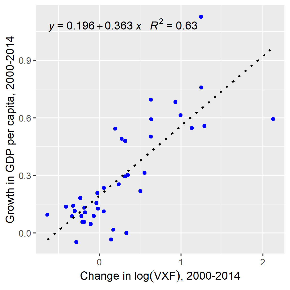
(a) VXF

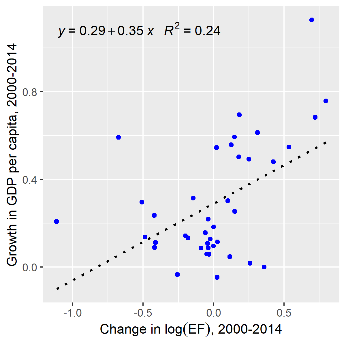
(b) EF

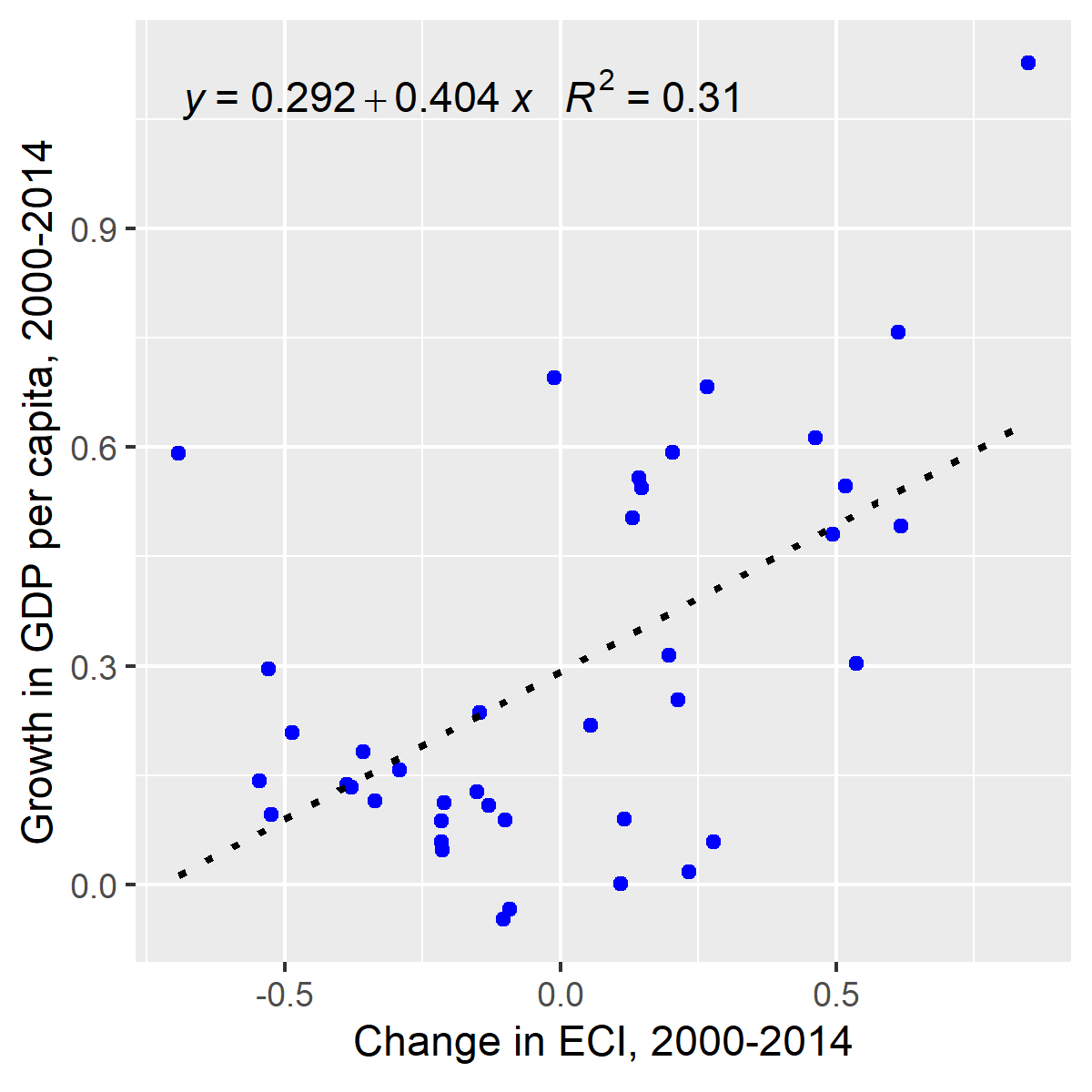
(c) ECI

Figure 1: Unconditional correlation between complexity and GDP per capita growth

For further investigation, I create a panel dataset including 40 lower-middle- to high-income countries and comprising three non-overlapping time periods: 2000-2004, 2005-2009, and 2010-2014. I estimate the following first-differenced growth model accounting for individual and time fixed effects

$$y_{i,t}-y_{i,t-4}=\alpha y_{i,t-4}+\beta_{1}(C_{i,t}-C_{i,t-4})+\beta_{2}C_{i,t-4}+\gamma X_{i,t}+\theta_{t}+(\epsilon_{i,t}-\epsilon_{i,t-4})\quad,$$ (6)

where $C$ denotes one of the three complexity metrics and $y$ the logarithmic GDP per capita. $X_{i,t}$ includes typical growth model covariates, i.e. population growth ($n$), change in capital ($K$), change in human capital ($H$), and the initial stock of human capital.

Columns (1)-(3) of Table 2 show the regression results. It shows that, on the one hand, the conditional correlation is stronger for $VXF$ than for metrics based on gross exports. On the other hand, including $VXF$ instead of $EF$ or $ECI$ heightens the explanatory power of the model considerably. Moreover, the lower point estimate for the initial human capital stock, if $VXF$ is included, may allow for the conclusion that complexity in terms of a country’s value-added export structure more accurately depicts capabilities.

Keeping in mind the caveats attached to dynamic panel models, I estimate a non-dynamic fixed effects model as a robustness check. Columns (4)-(6) in Table 2 show the results. While the impact of complexity in terms of gross exports on growth becomes insignificant in this specification, both for $EF$ and $ECI$, $VXF$ is still significantly correlated with economic growth.

Furthermore, the approximation of economic complexity based on value-added exports may be a source of endogeneity, since they directly represent a part of GDP. However, the iterative processes described in Equations 2 to 5 quantify the structure of an economy’s value-added exports. That is, an increase in value-added exports does not automatically lead to an increase in $VXF$. Rather, this depends on whether it positively affects the complexity of the value-added export basket, either by an increase in its diversification or by a further specialization in a complex industry (see Equation 1). To further support that the relationship between $VXF$ and GDP per capita growth is not driven by simply exporting more and thereby increasing value-added, I additionally control for a country’s trade openness. Table A.1 in the appendix shows that the results remain qualitatively unchanged, if holding trade openness constant.

	Dependent variable: $y_{i,t}-y_{i,t-4}$
	(1)	(2)	(3)	(4)	(5)	(6)
$y_{i,t-4}$	$-$0.254∗∗∗	$-$0.108∗∗∗	$-$0.120∗∗∗
	(0.062)	(0.038)	(0.044)
$n_{i,t}$	$-$0.044	0.476	0.179	$-$0.381	$-$0.193	$-$0.307
	(0.283)	(0.395)	(0.366)	(0.298)	(0.357)	(0.344)
$\Delta log(K)_{i,t}$	0.189∗∗∗	0.233∗∗∗	0.235∗∗∗	0.204∗∗∗	0.241∗∗∗	0.245∗∗∗
	(0.021)	(0.022)	(0.025)	(0.022)	(0.021)	(0.022)
$\Delta log(VXF)_{i,t}$	0.270∗∗∗			0.137∗∗∗
	(0.044)			(0.032)
$log(VXF)_{i,t-4}$	0.159∗∗∗
	(0.030)
$\Delta log(EF)_{i,t}$		0.112∗			0.073
		(0.068)			(0.067)
$log(EF)_{i,t-4}$		0.069∗∗
		(0.030)
$\Delta ECI_{i,t}$			0.090∗∗			0.045
			(0.036)			(0.033)
$ECI_{i,t-4}$			0.064∗∗
			(0.031)
$\Delta log(H)_{i,t}$	$-$0.099	$-$0.198	$-$0.045	$-$0.399	$-$0.717∗∗	$-$0.644∗∗
	(0.304)	(0.339)	(0.312)	(0.293)	(0.301)	(0.287)
$log(H)_{i,t-4}$	0.619∗∗∗	0.772∗∗∗	0.736∗∗∗
	(0.209)	(0.218)	(0.217)
Observations	120	120	120	120	120	120
R2	0.690	0.585	0.577	0.577	0.500	0.496
Adjusted R2	0.480	0.304	0.291	0.319	0.195	0.190

• Note: All regressions include individual and time fixed effects. Standard errors accounting for heteroskedasticity are applied. ^∗p$<$0.1; ^∗∗p$<$0.05; ^∗∗∗p$<$0.01

Table 2: Main regression results

4 Conclusion

This article contributes to the literature by providing a new perspective on complexity. Established metrics approximate an economy’s complexity by its gross export structure. I suggest using a country’s value-added export structure instead, since value-added exports are arguably a more reliable depiction of economic performance. Based on a weighted adjacency matrix and iterative processes analogous to Tacchella.2012 and Tacchella.2013, I introduce the value-added export Fitness ($VXF$) metric. I show that $VXF$, firstly, leads to substantially different complexity rankings compared to the established $ECI$ and $EF$ indices. That is, the United States top the rankings in terms of $VXF$, while Japan and China are the most complex countries in terms of $ECI$ and $EF$, respectively. Secondly, including $VXF$, instead of $ECI$ or $EF$, in a first-differenced growth model with fixed effects controlling for typical growth regression covariates, improves the explanatory power considerably.

Further research may rely on different inter-country Input-Output Tables to investigate a larger number of countries, including, specifically, more low- and middle-income countries. A larger sample may allow for a more robust econometric assessment of the effects of complexity on economic growth. Other currently available databases, however, use a coarser industry classification. Moreover, future research should more thoroughly investigate the interactions between human capital and complexity.

Appendix

List of countries (ISO 3166-1).

AUS, AUT, BEL, BGR, BRA, CAN, CHE, CHN, CYP, CZE, DEU, DNK, ESP, EST, FIN, FRA, GBR, GRC, HRV, HUN, IDN, IND, IRL, ITA, JPN, KOR, LTU, LVA, MEX, NLD, NOR, POL, PRT, ROU, RUS, SVK, SVN, SWE, TUR, USA.

	Dependent variable: $y_{i,t}-y_{i,t-4}$
	(1)	(2)	(3)	(4)	(5)	(6)
$y_{i,t-4}$	$-$0.278∗∗∗	$-$0.150∗∗∗	$-$0.185∗∗∗
	(0.057)	(0.037)	(0.037)
$n_{i,t}$	$-$0.001	0.487	0.168	$-$0.387	$-$0.265	$-$0.384
	(0.271)	(0.377)	(0.356)	(0.290)	(0.354)	(0.357)
$\Delta log(K)_{i,t}$	0.178∗∗∗	0.216∗∗∗	0.213∗∗∗	0.200∗∗∗	0.238∗∗∗	0.237∗∗∗
	(0.021)	(0.021)	(0.022)	(0.022)	(0.020)	(0.021)
$\Delta log(VXF)_{i,t}$	0.264∗∗∗			0.128∗∗∗
	(0.043)			(0.030)
$log(VXF)_{i,t-4}$	0.162∗∗∗
	(0.028)
$\Delta log(EF)_{i,t}$		0.081			0.044
		(0.063)			(0.062)
$log(EF)_{i,t-4}$		0.065∗∗
		(0.026)
$\Delta ECI_{i,t}$			0.118∗∗∗			0.056
			(0.037)			(0.035)
$ECI_{i,t-4}$			0.087∗∗∗
			(0.028)
$\Delta log(H)_{i,t}$	$-$0.226	$-$0.322	$-$0.242	$-$0.509∗	$-$0.825∗∗∗	$-$0.740∗∗
	(0.305)	(0.343)	(0.312)	(0.289)	(0.308)	(0.302)
$log(H)_{i,t-4}$	0.581∗∗∗	0.746∗∗∗	0.662∗∗∗
	(0.183)	(0.181)	(0.176)
$\Delta log(KOF)_{i,t}$	$-$0.081∗∗	$-$0.135∗∗∗	$-$0.152∗∗∗	$-$0.096∗∗∗	$-$0.116∗∗∗	$-$0.120∗∗∗
	(0.035)	(0.035)	(0.036)	(0.036)	(0.035)	(0.036)
Observations	117	117	117	117	117	117
R2	0.718	0.628	0.641	0.608	0.537	0.543
Adjusted R2	0.518	0.366	0.388	0.359	0.243	0.253

• Note In contrast to Table 2, these regressions do not include ROU due to availability of the trade openness indicator. All regressions include individual and time fixed effects. Standard errors accounting for heteroskedasticity are applied. ^∗p$<$0.1; ^∗∗p$<$0.05; ^∗∗∗p$<$0.01

Table A.1: Robustness check

References

- Balassa (\APACyear1965) \APACinsertmetastarBalassa.1965{APACrefauthors}Balassa, B. \APACrefYearMonthDay1965. \BBOQ\APACrefatitleTrade Liberalisation and Revealed Comparative Advantage Trade liberalisation and revealed comparative advantage.\BBCQ \APACjournalVolNumPagesThe Manchester School33299–123. {APACrefDOI} 10.1111/j.1467-9957.1965.tb00050.x \PrintBackRefs\CurrentBib
- Feenstra \BOthers. (\APACyear2015) \APACinsertmetastarFeenstra.2015{APACrefauthors}Feenstra, R\BPBIC., Inklaar, R.\BCBL \BBA Timmer, M\BPBIP. \APACrefYearMonthDay2015. \BBOQ\APACrefatitleThe Next Generation of the Penn World Table The next generation of the penn world table.\BBCQ \APACjournalVolNumPagesAmerican Economic Review105103150–3182. {APACrefDOI} 10.1257/aer.20130954 \PrintBackRefs\CurrentBib
- Gygli \BOthers. (\APACyear2019) \APACinsertmetastarGygli.2019{APACrefauthors}Gygli, S., Haelg, F., Potrafke, N.\BCBL \BBA Sturm, J\BHBIE. \APACrefYearMonthDay2019. \BBOQ\APACrefatitleThe KOF globalisation index–revisited The kof globalisation index–revisited.\BBCQ \APACjournalVolNumPagesThe Review of International Organizations143543–574. \PrintBackRefs\CurrentBib
- Hausmann \BOthers. (\APACyear2007) \APACinsertmetastarHausmann.2007{APACrefauthors}Hausmann, R., Hwang, J.\BCBL \BBA Rodrik, D. \APACrefYearMonthDay2007. \BBOQ\APACrefatitleWhat you export matters What you export matters.\BBCQ \APACjournalVolNumPagesJournal of Economic Growth1211–25. {APACrefDOI} 10.1007/s10887-006-9009-4 \PrintBackRefs\CurrentBib
- Hidalgo \BBA Hausmann (\APACyear2009) \APACinsertmetastarHidalgo.2009{APACrefauthors}Hidalgo, C\BPBIA.\BCBT \BBA Hausmann, R. \APACrefYearMonthDay2009. \BBOQ\APACrefatitleThe building blocks of economic complexity The building blocks of economic complexity.\BBCQ \APACjournalVolNumPagesPNAS1062610570–10575. \PrintBackRefs\CurrentBib
- Hidalgo \BOthers. (\APACyear2007) \APACinsertmetastarHidalgo.2007{APACrefauthors}Hidalgo, C\BPBIA., Klinger, B., Barabási, A\BHBIL.\BCBL \BBA Hausmann, R. \APACrefYearMonthDay2007. \BBOQ\APACrefatitleThe product space conditions the development of nations The product space conditions the development of nations.\BBCQ \APACjournalVolNumPagesScience (New York, N.Y.)3175837482–487. {APACrefDOI} 10.1126/science.1144581 \PrintBackRefs\CurrentBib
- Johnson \BBA Noguera (\APACyear2017) \APACinsertmetastarJohnson.2017{APACrefauthors}Johnson, R\BPBIC.\BCBT \BBA Noguera, G. \APACrefYearMonthDay2017. \BBOQ\APACrefatitleA Portrait of Trade in Value-Added over Four Decades A portrait of trade in value-added over four decades.\BBCQ \APACjournalVolNumPagesThe Review of Economics and Statistics995896–911. {APACrefDOI} 10.1162/REST_a_00665 \PrintBackRefs\CurrentBib
- Koopman \BOthers. (\APACyear2014) \APACinsertmetastarKoopman.2014{APACrefauthors}Koopman, R., Wang, Z.\BCBL \BBA Wei, S\BHBIJ. \APACrefYearMonthDay2014. \BBOQ\APACrefatitleTracing Value-Added and Double Counting in Gross Exports Tracing value-added and double counting in gross exports.\BBCQ \APACjournalVolNumPagesAmerican Economic Review1042459–494. {APACrefDOI} 10.1257/aer.104.2.459 \PrintBackRefs\CurrentBib
- Tacchella \BOthers. (\APACyear2012) \APACinsertmetastarTacchella.2012{APACrefauthors}Tacchella, A., Cristelli, M., Caldarelli, G., Gabrielli, A.\BCBL \BBA Pietronero, L. \APACrefYearMonthDay2012. \BBOQ\APACrefatitleA new metrics for countries’ fitness and products’ complexity A new metrics for countries’ fitness and products’ complexity.\BBCQ \APACjournalVolNumPagesScientific reports2723. {APACrefDOI} 10.1038/srep00723 \PrintBackRefs\CurrentBib
- Tacchella \BOthers. (\APACyear2013) \APACinsertmetastarTacchella.2013{APACrefauthors}Tacchella, A., Cristelli, M., Caldarelli, G., Gabrielli, A.\BCBL \BBA Pietronero, L. \APACrefYearMonthDay2013. \BBOQ\APACrefatitleEconomic complexity: Conceptual grounding of a new metrics for global competitiveness Economic complexity: Conceptual grounding of a new metrics for global competitiveness.\BBCQ \APACjournalVolNumPagesJournal of Economic Dynamics and Control3781683–1691. {APACrefDOI} 10.1016/j.jedc.2013.04.006 \PrintBackRefs\CurrentBib
- The Growth Lab at Harvard University (\APACyear2019) \APACinsertmetastarTheGrowthLabatHarvardUniversity.2019{APACrefauthors}The Growth Lab at Harvard University. \APACrefYear2019. \APACrefbtitleGrowth Projections and Complexity Rankings Growth projections and complexity rankings. {APACrefDOI} 10.7910/DVN/XTAQMC \PrintBackRefs\CurrentBib
- Timmer \BOthers. (\APACyear2015) \APACinsertmetastarTimmer.2015{APACrefauthors}Timmer, M\BPBIP., Dietzenbacher, E., Los, B., Stehrer, R.\BCBL \BBA de Vries, G\BPBIJ. \APACrefYearMonthDay2015. \BBOQ\APACrefatitleAn Illustrated User Guide to the World Input-Output Database: The Case of Global Automotive Production An illustrated user guide to the world input-output database: The case of global automotive production.\BBCQ \APACjournalVolNumPagesReview of International Economics233575–605. {APACrefDOI} 10.1111/roie.12178 \PrintBackRefs\CurrentBib
- Timmer \BOthers. (\APACyear2019) \APACinsertmetastarTimmer.2019{APACrefauthors}Timmer, M\BPBIP., Miroudot, S.\BCBL \BBA de Vries, G\BPBIJ. \APACrefYearMonthDay2019. \BBOQ\APACrefatitleFunctional specialisation in trade Functional specialisation in trade.\BBCQ \APACjournalVolNumPagesJournal of Economic Geography1911–30. {APACrefDOI} 10.1093/jeg/lby056 \PrintBackRefs\CurrentBib
- Wittgenstein Centre for Demography and Global Human Capital (\APACyear2018) \APACinsertmetastarWittgensteinCentreforDemographyandGlobalHumanCapital.2018{APACrefauthors}Wittgenstein Centre for Demography and Global Human Capital. \APACrefYear2018. \APACrefbtitleWittgenstein Centre Data Explorer Version 2.0 (Beta) Wittgenstein centre data explorer version 2.0 (beta). {APACrefURL} http://www.wittgensteincentre.org/dataexplorer \PrintBackRefs\CurrentBib