Parameter inference for a stochastic kinetic model of expanded polyglutamine proteins

Abstract

The presence of protein aggregates in cells is a known feature of many human age-related diseases, such as Huntington’s disease. Simulations using fixed parameter values in a model of the dynamic evolution of expanded polyglutamine (PolyQ) proteins in cells have been used to gain a better understanding of the biological system, how to focus drug development and how to construct more efficient designs of future laboratory-based in vitro experiments. However, there is considerable uncertainty about the values of some of the parameters governing the system. Currently, appropriate values are chosen by ad hoc attempts to tune the parameters so that the model output matches experimental data. The problem is further complicated by the fact that the data only offer a partial insight into the underlying biological process: the data consist only of the proportions of cell death and of cells with inclusion bodies at a few time points, corrupted by measurement error.

Developing inference procedures to estimate the model parameters in this scenario is a significant task. The model probabilities corresponding to the observed proportions cannot be evaluated exactly and so they are estimated within the inference algorithm by repeatedly simulating realisations from the model. In general such an approach is computationally very expensive and we therefore construct Gaussian process emulators for the key quantities and reformulate our algorithm around these fast stochastic approximations. We conclude by examining the fit of our model and highlight appropriate values of the model parameters leading to new insights into the underlying biological processes such as the kinetics of aggregation.

Keywords: Gaussian process emulator; history matching; MCMC; optimal design; stochastic kinetic model.

1 Introduction

One of the main aims of modelling biological systems is to describe and understand the temporal evolution of the system taking account of the potentially complex inter-relationships between components within the system. Models can also be used to facilitate in silico experiments in which virtual experiments are performed on a computer. These in silico experiments have an advantage over laboratory-based experiments as, in general, they are much cheaper and faster to conduct. This can lead to a better understanding of, for example, the biological system, how to focus drug development and how to construct more efficient designs of future laboratory-based in vitro experiments.

The accumulation of abnormal protein deposits within cells are hallmarks of neurodegenerative diseases affecting humans as they age. There are many such diseases, (e.g. Alzheimer’s and Parkinson’s disease), in which different parts of the brain are affected resulting in a range of clinical symptoms such as loss of motor function, dementia, and behavioural changes. Despite differences between symptoms, there are similarities in the underlying molecular mechanisms leading to the accumulation of protein aggregates and the neuronal cell death (Gan, Cookson et al. 2018). Although, age is the greatest risk factor for neurodegeneration, there is a group of diseases that are caused by genetic mutations. In nine of these diseases, the mutation occurs in a gene that contains a repeat of a CAG nucleotide triplet (Lieberman, Shakkottai et al. 2019). As CAG encodes for the amino acid glutamine, these diseases are known as polyglutamine diseases and the proteins they encode are referred to as PolyQ proteins, although different genes and proteins are involved in each disease, e.g. Huntington’s disease (HD), (Lieberman, Shakkottai et al. 2019). HD is an adult-onset, progressive disease characterised by loss of motor function, psychiatric disorders and dementia (McColgan and Tabrizi 2018). In this disease, the CAG triplet is found in the huntingtin gene (HTT, HGNC:4581). In the normal HTT gene, the CAG triplet is repeated 10-35 times but in the mutated form, the segment is expanded from 36 to over 120 repeats. This leads to the formation of an abnormally long protein which may be cleaved within the cell into small toxic fragments that enter the nucleus where they form aggregates, known as inclusion bodies (or inclusions), and sequester other proteins causing transcriptional dysregulation although the exact mechanisms of how this occurs are still unknown (McColgan and Tabrizi 2018). In addition, huntingtin fragments form aggregates in the cytoplasm and may impair cellular function, e.g. impairment of proteostasis (McColgan and Tabrizi 2018).

There are currently no effective interventions for the prevention, delay in onset or slowing down of disease progression in HD or in any other neurodegenerative disorder. This is mainly due to a lack of a full understanding of the underlying molecular mechanisms. In particular, although protein aggregation is a common feature of all these disorders, it is still not fully known how protein aggregates actually contribute to the disease process. There has been considerable controversy over which stage of the aggregation process is most toxic to cells, and it has been suggested that the formation of large inclusion bodies may be protective as they sequester misfolded proteins and prevent the overload of protein degradation pathways (Ross and Poirier 2004). This has been shown experimentally in cell culture (Arrasate, Mitra et al. 2004). However, this protective effect may only be short-term, as large aggregates also contain proteins involved in the removal and repair of damaged protein and it has been suggested that they may induce quiescence and induction of cell death via necrosis (Ramdzan, Trubetskov et al. 2017), which can cause damage to neighbouring cells. In addition, nuclear inclusions may impair redox signalling leading to an increase in oxidative stress and further damage (Paul and Snyder 2019). The controversy regarding cytoxicity of PolyQ proteins is largely due to insufficient understanding of the molecular mechanisms involved. This motivated our previous study which used live cell imaging with fluorescent reporter systems to examine the relationship between PolyQ protein, activation of the stress kinase p38MAPK (MAPK14; HGNC:6876 ), reactive oxygen species (ROS) generation, inhibition of the proteasome (a protein complex which degrades cellular proteins), and formation of PolyQ nuclear inclusions (Tang, Proctor et al. 2010). It was found that proteasome inhibition usually preceded formation of inclusion bodies and that p38MAPK inhibitors alleviated the inhibition of proteasomes and delayed the onset of inclusion formation. Conversely, the addition of proteasome inhibitors resulted in earlier formation of inclusions. This study also included a computational model which explored the complex interactions of PolyQ proteins with other elements of the cell and they used computer simulations from the model (with fixed parameter values) to suggest ways to reduce the toxicity of PolyQ proteins on cells. As their model describes dynamic interactions at the single cell level, the number of different biochemical species vary discretely over time, often with low copy numbers (Gillespie,, 1977). Also the interaction of the species is driven by Brownian motion and so accurate modelling requires that it take account of the inherent stochasticity present in the system.

Currently, plausible values for the parameters in the PolyQ model are determined by using model simulations for specified values of the parameters and then adjusting them in an attempt to match experimental data. Clearly this is a difficult task and one with which statisticians can make a contribution. The general scenario of modelling biological systems in computational systems biology is described by Kitano, (2001) with increasing focus on those describing the stochastic dynamics of individual cells (Elowitz et al.,, 2002; Swain et al.,, 2002). More recently an overview of this area has been provided by Villaverde and Banga, (2014).

A key difficulty in conducting parameter inference for complex stochastic models such as the PolyQ model is that the experimental data are typically incomplete and subject to measurement error. This necessitates the use of computationally intensive schemes such as Gibbs sampling (Boys et al.,, 2008), pseudo-marginal Metropolis-Hastings (Golightly and Wilkinson,, 2011; Georgoulas et al.,, 2016; Wilkinson,, 2018), population Monte Carlo (Koblents and Míguez,, 2015; Koblents et al.,, 2019) and approximate Bayesian computation (Wu et al.,, 2014; Owen et al.,, 2015). Inference is particularly challenging for the PolyQ model since the data consist only of the proportion of cells which are dead and the proportion of cells which contain inclusion bodies. Since the corresponding model probabilities are intractable, these latent proportions must be estimated at each observation time by repeatedly forward simulating the model over the duration of the time-course. Computational cost can be reduced by replacing the expensive and exact stochastic simulator with a cheap approximation. For example, approaches which replace the continuous-time stochastic model with a discrete-time approximation include tau-leaping (Gillespie,, 2001; Cao et al.,, 2006) and the chemical Langevin equation (Gillespie,, 2000; van Kampen,, 2001).

1.1 Contributions and organisation of the paper

The aim of this paper is to examine what insight the limited available experimental data provides about the PolyQ model parameters and to check whether the model gives a reasonable description of the dynamic variation observed in the experimental data.

Given the prohibitive computational cost associated with fitting the stochastic polyQ model, we consider a computationally feasible approximation and perform exact (simulation-based) inference for the resulting model. We eschew the use of an approximate simulator in favour of directly emulating the empirical logit of the proportions of interest with a Gaussian process (GP) (Rasmussen and Williams,, 2006; Santner et al.,, 2003). In particular, combining the fitted GP emulator with a Gaussian measurement model (on the same scale as the observed data) allows a direct approximation of the observed data likelihood without recourse to further simulation from the stochastic PolyQ model.

The findings from this analysis give new information regarding the parameters of the model, which in turn leads to new insights into the underlying biological processes. For example, this analysis has shown that during the first stages of the aggregation process both aggregation and disaggregation probably occur much faster and that the disaggregation/aggregation ratio is likely to be a magnitude higher than was originally assumed. The biological implication of this is that it will take longer to reach the threshold size required for inclusion formation but that there will also be higher levels of small aggregates which will inhibit the proteasome.

The remainder of the paper is organised as follows. Section 2 details the experimental data available and outlines how it was collected. A complete description of the model is given in section 3 which includes the underlying stochastic model which describes the dynamic evolution of this biological process and the observation model, which links the data to the underlying process. Our prior assumptions about parameter values and initial levels are given in 4. A method for determining the posterior distribution for model quantities is described in section 5 and, because a standard simulation-based MCMC solution is prohibitively expensive, we develop Gaussian process emulators in section 6 which facilitate timely generation of realisations from the posterior distribution. As we have high prior uncertainty on model parameters, in section 7 we employ a history matching technique which removes implausible training points in an attempt to fit the GPs within regions of non-negligible posterior support. We also include an assessment of the quality of the final fitted GPs. We present our findings about the the PolyQ model in section 8, and point out new insights into this biological system.

2 Experimental data

We have data from two different sets of experiments. These were carried out in the same laboratory and are described briefly below. A more comprehensive description of the experimental procedures can be found in Tang et al., (2010).

2.1 Cell death

The first experiment begins with a large number of human U87MG glioblastoma cells maintained in a suitable medium at 37^∘C at 5% CO₂. The cells are transfected with a construct that contains the expanded PolyQ Huntington protein (see section 2.2 for details). The survival of cells is monitored over time. Three different repeats of the experiment are carried out under the following experimental conditions:

1. Control group: No intervention.

2. Proteasome inhibition group: Cells are treated with a proteasome inhibitor 24 hours after transfection. The stochastic kinetic model captures this scenario by reducing the initial value $k_{proteff}=1$ to $k_{proteff}=0.05$ after 24 hours.

3. p38 inhibition group: Cells were pre-treated for 2 hours with a p38 inhibitor. The stochastic kinetic model captures this scenario by setting $k_{p38act}=0.05$.

The changes to parameter values used to describe the different experimental conditions were determined by conversations with the experimentalists. It was felt that reducing the rates to zero in conditions (ii) and (iii) overstated the effect of the experimental treatment and so these rates are set to low but non-zero values.

The cells are stained with propidium iodide, which is a fluorescent dye with the property that it only binds to non-viable (dead) cells. This technique is called propidium iodide exclusion and is used to identify the viability of the cells over time. The fluorescent dye can be viewed under a microscope and estimates of the proportion of cell death can be observed over time. These proportions of cell death form our experimental data which can be seen in Table 1. Each row of the table corresponds to experiments carried out under the different experimental conditions outlined above. We have two repeats of each experiment.

Within the stochastic model, cell death can occur via two biological pathways, either via proteasome inhibition or by p38 activation. This process is monitored within the model by using the dummy species PIdeath and p38death. These species are both binary variables, with a zero value representing that the cell is alive.

Table 1: Proportions of cell death observed under different experimental conditions.

Condition	24hrs	36hrs	48hrs
(i)	0.1503	0.1455	0.2608
	0.1788	0.1821	0.2846
(ii)	0.1897	0.1807	0.2250
	0.1640	0.1973	0.2998
(iii)	0.2168	0.2344	0.3644
	0.2436	0.2095	0.3872

2.2 Inclusion body formation

Experimentalists monitor the number of cells with inclusion bodies by first creating a construct that encodes an expanded PolyQ Huntington protein which is tagged with Yellow Fluorescent Protein (YFP). U87MG cells are transfected with the construct and then imaged at 10 minute intervals between 24 to 48 hours after transfection. Time lapse images reveal the formation of inclusions (by detecting YFP) and the percentage of cells with inclusions is recorded every 6 hours. The experimental results are given in Table 2. As with the data on cell death, each row corresponds to experiments carried out under different experimental conditions and we have two repeats of each experiment.

Within the stochastic model, the number of cells containing inclusions is counted via the number of cells containing SeqAggP. In the laboratory, image analysis suffers from a thresholding problem in detecting inclusions and we capture this aspect by defining cells with inclusions as those in which SeqAggP contains more than ten PolyQ proteins (i.e. $\texttt{SeqAggP}>10$). The value of this threshold is based on the biological modeller’s best understanding of the mechanism, though in fact the actual value is not crucial since aggregates grow very rapidly and there is only a very small timeframe when SeqAggP is less than ten.

Table 2: Proportions of inclusion bodies observed under different experimental conditions.

Condition	24hrs	30hrs	36hrs	42hrs	48 hrs
(i)	0.0909	0.2857	0.3824	0.4286	0.7273
	0.0175	0.2131	0.3538	0.4304	0.5742
(ii)	0.0909	0.4247	0.6125	0.7403	0.8194
	0.1154	0.5075	0.7895	0.8667	0.9157
(iii)	0.0303	0.0444	0.0612	0.1373	0.2200
	0.0189	0.0938	0.1286	0.1613	0.1833

3 The stochastic model

3.1 PolyQ mechanism

The stochastic model for the PolyQ mechanism we consider in this paper is a reduced form of that proposed by Tang et al., (2010). The original model developed by Tang et al. (Tang, Proctor et al. 2010) was constructed in the Systems Biology Markup Language (SBML) and is available from the Biomodels database (Li, Donizelli et al. 2010) (Model ID: BIOMD0000000285). The model was developed to investigate the effects of PolyQ on proteasome function, oxidative stress, and cell death. It contained a pool of PolyQ which was continually turned over, being degraded by the proteasome. It was assumed that the PolyQ aggregation process started by two monomers interacting, which then interacts with further monomers causing the aggregate to grow (AggPolyQ1-5). At early stages, it was assumed that disaggregation could also take place but that when the aggregate reached a threshold size (denoted by SeqAggP in the model), disaggregation does not take place, so that the aggregate continues to grow and an inclusion forms. The model also included a generic pool of protein which could be damaged by ROS leading to misfolding and aggregation. It was assumed that small aggregates bind to the proteasome but cannot be degraded and so inhibit proteasome function. In addition, they may increases levels of ROS. The model also included the stress kinase p38MAPK (simply modelled as two pools: inactive [p38] and active [p38P]) with activation occurring more frequently when levels of ROS are high (Sato, Okada et al. 2014), and that high levels of p38P activated a cell death pathway (denoted by p38death). Proteasomes bound by aggregates (AggPProteasome) could also activate a cell death pathway (denoted by PIdeath). The model also included the turnover of a fluorescent protein (mRFPu) as an increase in mRFPu levels indicates that the proteasome is inhibited, shown by live cell imaging in Tang et al. 2010. An example of this data is shown in Figure1.

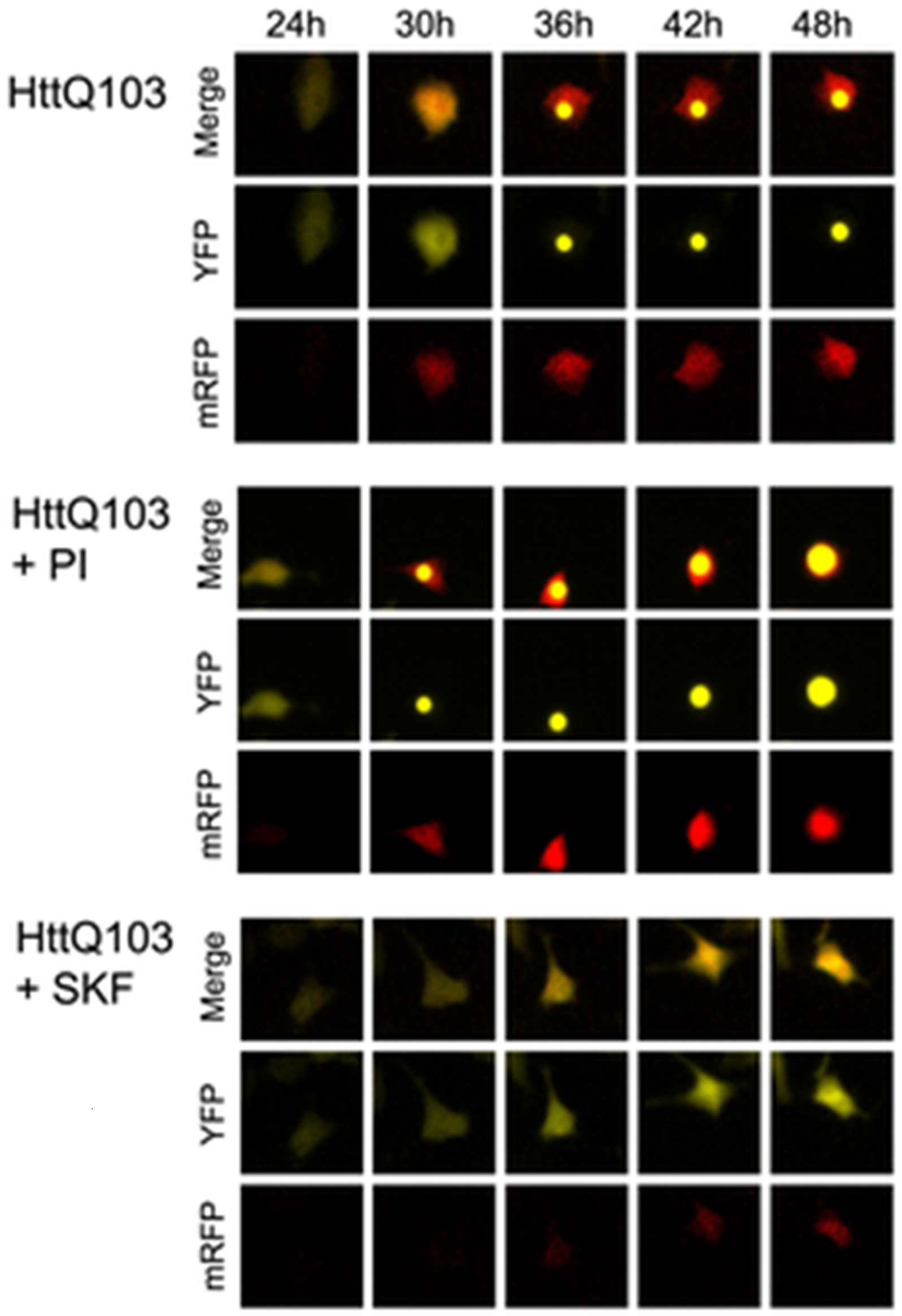
Figure 1: Example data from live cell imaging.

Given the complexity of the original model (with 27 chemical species and 72 reactions) it was necessary to consider a simplification for this study. The changes to the Tang model have been to reduce the number of species and reactions by removing the generic pool of protein and its associated reactions of misfolding and aggregation, and by removing the fluorescent protein mRFPu, which had been originally included as a marker of proteasome function. In the process of model construction, it was found neccesary to add in an effect of ROS on the aggregation process. The experimental biologists suggested that ROS increases the propensity of PolyQ proteins to aggregate due to ROS interfering with the ubiquitin-proteasome system (UPS), so that PolyQ proteins are more likely to aggregate than be degraded when ROS levels are high. The exact mechanism is not fully understood and so we simply included ROS in the rate laws for PolyQ aggregation.

The resulting reduced model contains 14 chemical species and 33 reaction channels, which is still relatively large when compared to other stochastic kinetic models for which fully Bayesian inference is available in the literature (Boys et al.,, 2008; Henderson et al.,, 2010). A complete list of the reactions and their stochastic rate laws describing the PolyQ model can be found in Appendix A of the Supplementary Materials. All reactions except those relating to aggregation follow the law of mass action kinetics. We used a Hill function for the effects of ROS as it is thought that low levels of ROS would have little effect on the UPS with a maximal effect when ROS levels are high. We assumed that the rate of aggregation would be half the maximal rate when ROS is at its basal level, which is achieved by using the value 10 in the denominator of the rate law.

The model is represented graphically in Figure 2, where oval shapes (nodes) represent chemical species and an arrow between two nodes represents a reaction which can take place involving the two chemical species. The figure clearly shows the complex interlinkages and complex feedback loops within the model.

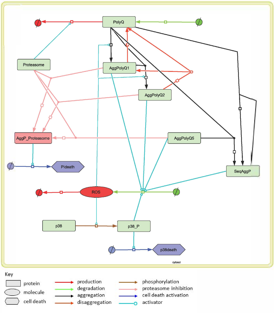
Figure 2: Network diagram of the PolyQ model

3.2 The observation model

We assume that the experimental data are noisy versions of the equivalent quantities in the stochastic model and adopt a simple model for this observation error which is additive independent normal noise on a logit scale (as the data are proportions). Other error models are possible, such as embedding the model probabilities within a Beta distribution, but this logistic normal model affords advantages in the subsequent analysis.

Suppose the stochastic model for the experiment run under condition $c$ with parameter vector $\boldsymbol{\theta}$ gives $p_{t,c}^{D}(\boldsymbol{\theta})$ and $p_{t,c}^{I}(\boldsymbol{\theta})$ as the probabilities of death and of the presence of inclusions at time $t$ and the logits of their observed versions as $y^{D}_{t,c,r}$ and $y^{I}_{t,c,r}$ in experimental repeat $r$. We assume the observation model is, for $c=1,2,3$, $r=1,2$

$$y^{D}_{t_{i},c,r} =\text{logit}\,p_{t_{i},c}^{D}(\boldsymbol{\theta})+\sigma_{D}\varepsilon_{i,c,r},\quad i=1,2,3$$

$$y^{I}_{t_{i},c,r} =\text{logit}\,p_{t_{i},c}^{I}(\boldsymbol{\theta})+\sigma_{I}\varepsilon_{i,c,r}^{*},\quad i=1,\ldots,5$$

where the $\varepsilon_{i,c,r}$ and $\varepsilon_{i,c,r}^{*}$ are i.i.d. standard normal quantities and $t_{i}$ denote the $i$th time-point at which an observation is available. Note that this model assumes the same measurement error distribution for each experimental condition and repeat. The implications of this observation model on the probability scale is explored in Appendix B of the Supplementary Materials.

4 Prior information

Tables 3 and 4 contain a list of all parameters in the model. Some parameters are known quite accurately in the literature. For example, the synthesis and degradation rates of PolyQ proteins $k_{synPolyQ}$ and $k_{degPolyQ}$ can be obtained by considering the half-life of PolyQ proteins (Persichetti et al.,, 1996).

Table 3: Parameters in the PolyQ model under condition (i) with their known values

Parameter	Value	Units	Reference
$k_{synPolyQ}$	$0.25$	molecule $s^{-1}$	Calculated from value of $k_{degPolyQ}$ to give
			steady state level of 1000 molecules
$k_{degPolyQ}$	$2.5\times 10^{-7}$	molecule${}^{-1}s^{-1}$	Half-life of $30$ hours (Persichetti et al., 1996)
$k_{actp38}$	$2\times 10^{-3}$	molecule${}^{-1}s^{-1}$	Phosphorylation occurs within
			(Aoki,Takahashi et al. 2013)
$k_{p38act}$	1.0	dimensionless	Dummy variable (set to $0.05$ for p38 inhibition)
$k_{proteff}$	1.0	dimensionless	Dummy variable (set to $0.05$ for proteasome
			inhibition)

Table 4: Parameters in the PolyQ model under condition (i) with their prior distribution.

Parameter	Prior distributions
$k_{aggPolyQ}$	$\theta_{1}=\log k_{aggPolyQ}\sim N(\log 10^{-7},5)$
$k_{disaggPolyQ_{1}}$	$\theta_{2}=\log k_{disaggPolyQ_{1}}\sim N(\log(5\times 10^{-7}),5)$
$k_{seqPolyQ}$	$\theta_{3}=\log k_{seqPolyQ}\sim N(\log(8\times 10^{-7}),5)$
$k_{inhprot}$	$\theta_{4}=\log k_{inhprot}\sim N(\log(5\times 10^{-9}),5)$
$k_{remROS}$	$\theta_{5}=\log k_{remROS}\sim N(\log(2\times 10^{-4}),5)$
$k_{genROSSeqAggP}$	$\theta_{6}=\log k_{genROSSeqAggP}\sim N(\log(10^{-7}),5)$
$k_{genROSAggP}$	$\theta_{7}=\log k_{genROSAggP}\sim N(\log(5\times 10^{-6}),5)$
$k_{inactp38}$	$\theta_{8}=\log k_{inactp38}\sim N(\log 0.8,5)$
$k_{genROSp38}$	$\theta_{9}=\log k_{genROSp38}\sim N(\log(7\times 10^{-7}),5)$
$k_{p38death}$	$\theta_{10}=\log k_{p38death}\sim N(\log(9\times 10^{-8}),5)$
$k_{PIdeath}$	$\theta_{11}=\log k_{PIdeath}\sim N(\log(2.5\times 10^{-8}),5)$
$\sigma_{D}$	$\sigma_{D}\sim InvChi(2,0.12)$
$\sigma_{I}$	$\sigma_{I}\sim InvChi(0.75,0.05)$

Also, to reduce the number of parameters in the model, it was thought reasonable to fix some rates to be identical to others or to be functions of other rates. For example, the disaggregation rates for different sized PolyQ aggregates have been fixed as known proportions of the rate for single PolyQ aggregates: $k_{disaggPolyQ2}=0.8\,k_{disaggPolyQ1}$, $k_{disaggPolyQ3}=0.6\,k_{disaggPolyQ1}$, and so on. In each case, these identities or fixed proportions have been chosen according to the biological modeller’s best understanding of the reaction system.

Only limited information is available for the remaining stochastic rate parameters and we represent these fairly weak prior beliefs using independent log-normal distributions with medians set at our biological modeller’s best guess. On the log scale, the kinetic rate parameters are denoted by $\theta_{1},\ldots,\theta_{11}$ and these parameters have independent normal prior distributions. The weak beliefs are represented by prior variances of five on the log scale as these correspond to a plausible range of values for the (untransformed) kinetic rates from 0.01 to 100 times their median value.

We have prior beliefs for the level of measurement error in the cell death experiments ($\sigma_{D}$) from time course data on two independent replicates from an independent (but similar) study measuring cell death proportions. The difference between these replicates on the logit scale form a random sample from a $N(0,\sigma_{D}^{2})$ distribution and so these logit differences lead to an inverse gamma posterior for $\sigma_{D}^{2}$ under a vague prior. This posterior corresponds to an inverse chi distribution for $\sigma_{D}$, where this distribution is defined as that of $1/\sqrt{X}$, where $X$ has a gamma distribution. Further, as these data arise from a similar but different study, we choose to construct our prior as a powered down version of this inverse chi posterior as this makes it more diffuse around an appropriate value (Ibrahim and Chen,, 2000). Our knowledge about the level of measurement error in the inclusion body experiments is weaker and so we use an even more powered down prior for $\sigma_{I}$.

There is also uncertainty about some of the initial levels of the different species. This uncertainty is captured by independent prior distributions elicited from the biological modeller. Other specie levels are known due to the construction of the experiment, such as those for AggPolyQ₁–AggPolyQ₅, others obey a conservation law ($\texttt{p38}+\texttt{p38P}=100$) and some levels, such as that for this conservation level and for PolyQ, set at fairly arbitrary high values reflecting the relative abundance of these species within the cell. The values or prior distribution of the initial levels are listed in Table 5. Note that two of these initial levels have a discrete log-normal $DLN$ prior distribution, with probability function $\pi(i)=Pr(i-0.5<X<i+0.5)$, where $X$ is a log-normal random variable.

Table 5: Value or prior distribution of the initial levels of the chemical species

Name	Value or prior distribution
PolyQ	1000
Proteasome	$DLN(6.9,0.1^{2})$
AggPolyQ1-5	0
SeqAggP	0
AggPProteasome	0
ROS	$DLN(2.5,0.25^{2})$
p38P	$U\{0,1,\ldots,5\}$
p38	100-p38P
PIdeath	0
p38death	0

5 Posterior inference

Knowledge of the kinetic rates $\boldsymbol{\theta}$ and the observation error levels $\boldsymbol{\sigma}=(\sigma_{D},\sigma_{I})$ is summarised in the posterior distribution, which has density

$$\pi(\boldsymbol{\theta},\boldsymbol{\sigma}|\boldsymbol{y})\propto\pi(\boldsymbol{\theta})\pi(\boldsymbol{\sigma})\pi(\boldsymbol{y}|\boldsymbol{\theta},\boldsymbol{\sigma}),$$

where $\boldsymbol{y}$ represents the collection of all data on cell death and inclusions. Although the normal likelihood has a simple form, it does require calculation of the probabilities $p_{t,c}^{D}(\boldsymbol{\theta})$ and $p_{t,c}^{I}(\boldsymbol{\theta})$. Unfortunately analytic expressions for these probabilities are not available due to the complexity of the stochastic model. Prior uncertainty around the initial specie levels $\boldsymbol{x}_{0}$ is a further complicating factor as, for example, $p_{t,c}^{D}(\boldsymbol{\theta})=E_{\boldsymbol{x}_{0}}\{p_{t,c}^{D}(\boldsymbol{\theta},\boldsymbol{x}_{0})\}$, where $E_{\boldsymbol{x}_{0}}\{\cdot\}$ denotes expectation with respect to $\boldsymbol{x}_{0}$. Therefore we estimate these probabilties using $n$ independent realisations of the stochastic model, initialised according to the prior distribution on initial levels. Suppose that a typical probability is estimated by the proportion $\widehat{p}_{n}$. For sufficiently large $n$, the empirical logit of such proportions $\text{elogit}\,\widehat{p}_{n}=\log\{(\widehat{p}_{n}+0.5/n)/(1-\widehat{p}_{n}+0.5/n)\}$ is unbiased for $\text{logit}~{}p$ and its sampling variability is closely described by a normal distribution with variance $1/\{n\widehat{p}_{n}(1-\widehat{p}_{n})\}$. Thus, taking an improper constant prior for $\text{logit}~{}p$ gives its posterior distribution as a normal distribution with mean $\text{elogit}\,\widehat{p}_{n}$ and variance $1/\{n\widehat{p}_{n}(1-\widehat{p}_{n})\}$. Therefore we can integrate out posterior uncertainty about $\text{logit}~{}p$ in the observation model, modifying it to have independent components of the form

$$y\sim N\bigl{(}\text{elogit}\,\widehat{p}_{n}(\boldsymbol{\theta}),~{}\sigma^{2}+1/[n\,\widehat{p}_{n}(\boldsymbol{\theta})\{1-\widehat{p}_{n}(\boldsymbol{\theta})\}]\bigr{)}.$$

Building an MCMC inference scheme around this normal likelihood is straightforward. We found that estimating the probabilities using $n=1000$ model simulations gave empirical logits which fitted well to a normal distribution. Note that, in order for these estimates to be uncorrelated, they have each been calculated using independent realisations of the model.

Unfortunately the MCMC scheme requires the generation of many millions (or even billions) of realisations from the stochastic model as it explores the posterior distribution. Clearly this problem prohibits using such a scheme for obtaining realisations from the posterior distribution in a timely manner. In such situations it is commonplace to use stochastic approximations for these deterministic model probabilities. We will use Gaussian process (GP) approximations (sometimes called emulators) which are popular in the deterministic computer model literature and elsewhere. Useful background articles in this area are Santner et al., (2003) and Bayarri et al., (2007). The suitability of GPs as emulators is highlighted in O’Hagan, (2006). Also see Henderson et al., (2009) for an illustration of the utility of GP emulators in the analysis of complex biological models.

6 Emulation

We need to build GP emulators approximating the stochastic output of the proportion of cell death and that of inclusions under the three different conditions. Time ($t$) is an input variable in these six emulators, in addition to the unknown stochastic rate constants ($\boldsymbol{\theta}$) and observation error levels ($\boldsymbol{\sigma}$). However, it can be problematic to specify appropriate covariance kernels over time. In any case, for Bayesian inference, all that is needed are emulators for the distributions of the probabilities under each experimental condition at the distinct time points ocurring in the datasets. Therefore we will build a total of 24 emulators: 9 for proportions of cell death and 15 for proportions of inclusion bodies. Using these time-condition-specific emulators also has the advantage that they can be built in parallel. Thus we build GP emulators for

$$x_{t_{i},c}^{D}(\boldsymbol{\theta}) =\text{elogit}\,\widehat{p}_{t_{i},c}^{D}(\boldsymbol{\theta})\quad i=1,2,3$$

and

$$x_{t_{i},c}^{I}(\boldsymbol{\theta}) =\text{elogit}\,\widehat{p}_{t_{i},c}^{I}(\boldsymbol{\theta})\quad i=1,\ldots,5,$$

for each condition $c=1,2,3$. The aim is to replace the empirical proportions in the observation model with GP emulators, allowing for their uncertainty. Fortunately this is straightfoward as each emulator prediction is also normally distributed and so, as before, the additional uncertainty introduced by the GPs can be integrated out analytically and there is no need for the MCMC scheme to integrate over an additional latent layer within the model.

6.1 Training data

In order to build the emulators for the $x_{t_{i},c}^{D}(\boldsymbol{\theta})$ and $x_{t_{i},c}^{I}(\boldsymbol{\theta})$, we first need to evalute their values at some set of chosen values for $\boldsymbol{\theta}$. This amounts to choosing the size and values in an $n_{d}$-point design $\boldsymbol{\Theta}=(\boldsymbol{\theta}_{1},\ldots,\boldsymbol{\theta}_{n_{d}})$. In common with other work in this area (Santner et al.,, 2003; Henderson et al.,, 2010) we choose to base our design on a Latin hypercube design (LHD) constructed using the maximin algorithm of Morris and Mitchell, (1995). These designs are popular as they produce an effective and efficient coverage of a bounded space. We take the bounded space to be the central hypercube of the prior distribution defined by the marginal 99% intervals for the rates $\theta_{j}$. Inevitably, determining an appropriate design from which to contruct GP emulators is a sequential process. This is because it is not unusual to find that there are only a few design points in the region of high posterior support, particularly when the marginal priors have large uncertainty (as we have here). To help with this problem, as part of the sequential building of the emulators, we filter out design points which are implausible (inconsistent with the data) by using a history matching technique (see section 7). Note that obtaining estimates at each point in the LHD for the proportions of cell death and of inclusions over repeated simulations of the stochastic model is easily parallelisable on a high performance computer system.

6.2 Mean function and covariance function

The mean function was taken as a linear predictor in the components of $\boldsymbol{\theta}$, with the least squares estimates as the coefficients. Thus each emulator has a mean function at input $\boldsymbol{\theta}=(\theta_{1},\ldots\theta_{11})^{T}$ of the form

$$m(\boldsymbol{\theta})=\hat{\beta}_{0}+\sum_{i=1}^{11}\hat{\beta}_{i}\theta_{i}.$$

This choice was taken to give a parsimonious yet reasonably well fitting mean function and essentially leaves the residuals to this fit being modelled by a zero mean function Gaussian process. As is commonly used in the emulation literature, we specified a squared exponential covariance function, with

$$K(\boldsymbol{\theta}_{i},\boldsymbol{\theta}_{j}|a,\boldsymbol{r})=a\exp\left\{-\sum_{k=1}^{11}r_{k}^{2}(\theta_{ik}-\theta_{jk})^{2}\right\}$$

where, for example, $\theta_{ik}$ denotes the $k$th component of $\boldsymbol{\theta}_{i}$. The parameters of this function control the overall level of variability and smoothness of the process, with smaller values of the inverse length scales $r_{k}$ giving smoother realisations.

6.3 Hyperparameter estimation

The hyperparameters $a$ and $\boldsymbol{r}=(r_{i})$ for each emulator need to be estimated from the training data before we can use them as part of the MCMC inference scheme. When fitting a typical GP to training data $\boldsymbol{x}(\boldsymbol{\Theta})=(x(\boldsymbol{\theta}_{1}),\ldots,x(\boldsymbol{\theta}_{n_{d}}))^{T}$, the likelihood for the hyperparameters results from $\boldsymbol{x}(\boldsymbol{\Theta})|a,\boldsymbol{r}\sim N_{n_{d}}(\boldsymbol{m}(\boldsymbol{\Theta}),K(\boldsymbol{\Theta},\boldsymbol{\Theta}|a,\boldsymbol{r}))$ where $N_{n_{d}}(\cdot,\cdot)$ denotes an $n_{d}$-dimensional Gaussian distribution and $K(\boldsymbol{\Theta},\boldsymbol{\Theta}|a,\boldsymbol{r})_{ij}=K(\boldsymbol{\theta}_{i},\boldsymbol{\theta}_{j}|a,\boldsymbol{r})$. In general it is not possible to obtain a posterior distribution in closed form for a prior on $(a,\boldsymbol{r})$. Here we take independent weak log-normal prior distributions for the hyperparameters, with $a\sim\text{LN}(0,100)$ and $r_{i}\sim\text{LN}(0,100)$, $i=1,\ldots,11$. The GPs were fitted by using the ‘no-U-Turn’ Hamiltonian Monte Carlo sampler and implemented via the RStan package interface to the Stan package (Carpenter et al.,, 2017; Stan Development Team,, 2018).

6.4 Modified observation model

For a typical GP, the prediction at a point $\boldsymbol{\theta}^{\dagger}$ has distribution

$$x(\boldsymbol{\theta}^{\dagger})\sim N(m^{*}(\boldsymbol{\theta}^{\dagger}),v^{*}(\boldsymbol{\theta}^{\dagger}))$$ (1)

where

$$m^{*}(\boldsymbol{\theta}^{\dagger}) =m(\boldsymbol{\theta}^{\dagger})+K(\boldsymbol{\theta}^{\dagger},\boldsymbol{\Theta})K(\boldsymbol{\Theta},\boldsymbol{\Theta})^{-1}\{\boldsymbol{x}(\boldsymbol{\Theta})-\boldsymbol{m}(\boldsymbol{\Theta})\}$$

$$v^{*}(\boldsymbol{\theta}^{\dagger}) =K(\boldsymbol{\theta}^{\dagger},\boldsymbol{\theta}^{\dagger})-K(\boldsymbol{\theta}^{\dagger},\boldsymbol{\Theta})K(\boldsymbol{\Theta},\boldsymbol{\Theta})^{-1}K(\boldsymbol{\theta}^{\dagger},\boldsymbol{\Theta})^{T}.$$

Strictly speaking, this emulator distribution is a function of the GP hyperparameters and so we should average over their posterior uncertainty. However, we have found that there is little gain in doing this over using a delta approximation in which the hyperparameters are fixed at their posterior mean.

We can incorporate the stochastic approximation of the GP emulator to $\text{elogit}~{}\widehat{p}_{n}$ into our observation model and integrate it out to give a model with independent components of the form

$$y\sim N\bigl{(}m^{*}(\boldsymbol{\theta}),~{}\sigma^{2}+v^{*}(\boldsymbol{\theta})+1/[n\,p^{*}_{n}(\boldsymbol{\theta})\{1-p^{*}_{n}(\boldsymbol{\theta})\}]\bigr{)}$$

where

$$p^{*}_{n}(\boldsymbol{\theta})=\text{eexpit}(\boldsymbol{\theta})=\{e^{m^{*}(\boldsymbol{\theta})}(1+0.5/n)-0.5/n\}/\{1+e^{m^{*}(\boldsymbol{\theta})}\}$$

is the GP prediction at point $\boldsymbol{\theta}$ on the probability scale.

7 History matching and validation

It is quite likely that large parts of parameter space will give rise to model outputs which are incompatible with the observed proportions. In practice, we need our Gaussian processes to be accurate over regions of parameter space with non-negligible posterior support and so time spent fitting them in regions of negligible posterior support is wasted. We can target the building of our GPs within regions of non-negligible posterior support using methods known as history matching (Cumming and Goldstein,, 2010; Vernon et al.,, 2014). These methods work by determining which design points are implausible before undertaking the computationally intensive task of evaluating the model output (here empirical logits) at these points. After fitting a GP over, implausible design points are determined by comparing data points $y_{i}$ with their GP prediction. An implausibility measure at data point $y_{i}$ takes the form

$$I_{i}(\boldsymbol{\theta})=\frac{|y_{i}-m^{*}(\boldsymbol{\theta})|}{\sqrt{\sigma^{2}+v^{*}(\boldsymbol{\theta})+1/[n\,p^{*}_{n}(\boldsymbol{\theta})\{1-p^{*}_{n}(\boldsymbol{\theta})\}]}}.$$

Adopting a conservative strategy, the implausibility measure over the entire data set is calculated as $I(\boldsymbol{\theta})=\max_{i}I_{i}(\boldsymbol{\theta})$. Large values of $I(\boldsymbol{\theta})$ indicate that $\boldsymbol{\theta}$ is an implausible point in parameter space. It is common to declare points as implausible if $I(\boldsymbol{\theta})>3$, this threshold being determined using Pukelsheim’s 3-sigma rule. Notice that the implausibility measure requires a value to be given for the measurement error level. We take the upper 1% value of its prior distribution ($\sigma_{D}=0.58$) as this possibly overestimates $\sigma_{D}$ and in doing so lowers the chance of incorrectly declaring a point as implausible whilst still ruling out a significant proportion of parameter space.

7.1 Iterative fitting of Gaussian processes

We used a sequential procedure for fitting the Gaussian process in order to make best use of the limited computing resources available to simulate realisations from the stochastic model (Figure 3). In what follows, we provide a brief description of this procedure and refer the reader to Appendix C of the Supplementary Materials for further details.

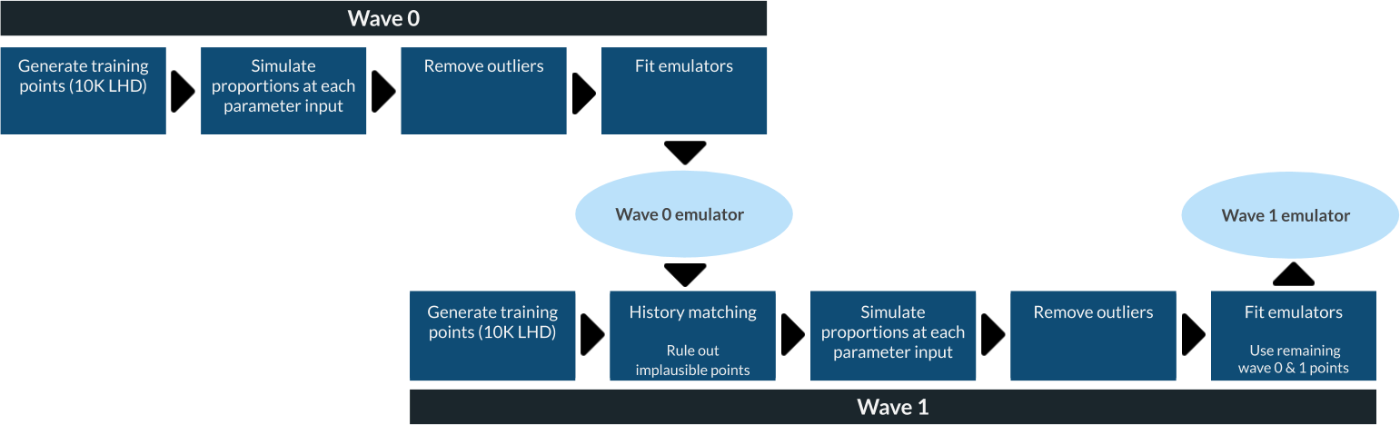
Figure 3: Flow chart showing the work flow involved in iteratively fitting Gausian process emulators.

We began in Wave 0 of the fitting procedure by constructing a 10K-point LHD within the cuboid defined by the 11 univariate marginal 99% prior equi-tailed intervals for each parameter $\theta_{j}$. Multiple realisations $(n=1000)$ were then obtained from the stochastic model at these design points to determine the empirical logit proportions of cell death and of inclusion bodies. Next we eliminated those design points which gave proportions (of cell death or of inclusion bodies) outside the range $(0.01,0.99)$, as such values look to be inconsistent with the data and they take considerable computing time to obtain. Finally, in Wave 0, we fitted a Gaussian process ($GP_{0}$) to the remaining 415 training points. Next, in Wave 1, we constructed an additional 10K-point LHD and removed any design points which had predicted probabilities (of the form $\text{eexpit}\{m^{*}_{GP_{0}}(\boldsymbol{\theta}_{i})\}$) outside $(0.01,0.99)$. The points surviving Wave 0 were then added and any points with implausibilities $I_{GP_{0}}(\boldsymbol{\theta}_{i})>3$ removed. Note that these implausibilities were calculated using the Gaussian processes $GP_{0}$ fitted at the end of Wave 0. Multiple realisations from the stochastic model were then simulated at the remaining 429 design points, empirical logits calculated and Gaussian processes $GP_{1}$ fitted to this output. In practice, this process could be repeated to give many more waves of history matching, and thereby narrow down the plausible parameter space even further. However, due to our limited computer resources, we terminated our process with $GP_{1}$.

7.2 Emulator validation

Before using the $GP_{1}$ emulators as part of the inference scheme it is important to verify that they provide an adequate description of model realisations of the empirical logits. There are a variety of diagnostic checks available based on comparisons of realisations from the stochastic model at a new set of design points ($\boldsymbol{\theta}^{\dagger}_{i}$) and comparing these with predictions made from the emulators; see, for example, Bastos and O’Hagan, (2009) and Gneiting et al., (2007).

We constructed a validation design of a similar size to that used for fitting the $GP_{{\color[rgb]{0,0,0}1}}$ emulators by repeating the Wave 0–1 procedure described in the previous section. This approach gives an independent design but still contains points in regions of non-negligible posterior support, where we most need the emulators to fit well. For each Gaussian process, we calculated individual prediction errors (IPEs) at each design point as $D(\boldsymbol{\theta}^{\dagger}_{i})=\{x(\boldsymbol{\theta}_{i}^{\dagger})-m^{*}(\boldsymbol{\theta_{i}}^{\dagger})\}/\surd{v^{*}(\boldsymbol{\theta}^{\dagger}_{i})}$, where $x(\boldsymbol{\theta}_{i}^{\dagger})$ is an empirical logit (for a particular time-condition proportion) calculated from $n=1000$ runs of the stochastic model with rates $\boldsymbol{\theta}=\boldsymbol{\theta}_{i}^{\dagger}$. Individual values of $D(\boldsymbol{\theta}^{\dagger}_{i})$ are informative about emulator fit but it is particularly instructive to look at their overall distribution. If the assumptions underpinning the emulator are appropriate then the $D(\boldsymbol{\theta}^{\dagger}_{i})$ values should be a random sample from a standard normal distribution. In particular, we would expect that roughly $95\%$ of the IPE values are within the interval $(-2,2)$. If the magnitude of the IPE is too large, this indicates that, at this input point, the emulator either fits poorly or its variability is underestimated. Conversely, too many very small values are indicative of an inflated emulator variance. Gneiting et al., (2007) suggest that checks also be made using the probability integral transform (PIT) to assess the (standard) normality of the $D(\boldsymbol{\theta}^{\dagger}_{i})$ as, if this holds, values of $\Phi\{D(\boldsymbol{\theta}_{i}^{\dagger})\}$ should form a random sample from a standard uniform distribution, where $\Phi(\cdot)$ is the standard normal distribution function. The IPEs for all 24 time-condition emulators are shown in Figure 4. Rather than produce additional PIT plots we give boxplot summaries for each emulator and include horizontal lines showing the positions of the quartiles and upper and lower 2.5% points of the standard normal distribution.

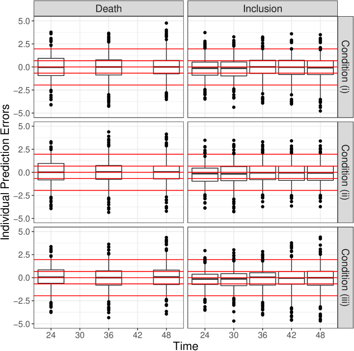
Figure 4: Boxplots of the individual prediction errors for each emulator together with horizontal lines showing the position of the quartiles and upper and lower 2.5% points of the standard normal distribution.

These and other plots (see Appendix D of the Supplementary Materials) suggest that there are no strong departures from the univariate normal assumptions (1) used to form the likelihood function.

8 Posterior summaries and conclusions

To construct the emulators, training data (consisting of stochastic realisations from the model) were generated in parallel on a high performance computer (HPC), with 64 compute nodes, where each node had at least 128GB of RAM and a minimum processor speed of 2.5GHz. Hyper-parameter inference was performed via the RStan interface to Stan, on a different HPC (with 23 cores and a minimum processor speed of 2.70GHz). The total CPU time to obtain the fitted emulators was approximately 1 day.

Realisations from the joint posterior distribution of all parameters of interest were obtained by using the fitted emulators and again implemented via the RStan interface to Stan.

This MCMC algorithm uses the ‘no-U-Turn’ Hamiltonian Monte Carlo sampler which efficiently explores the parameter space to maximise mixing. We ran three chains, each for 100K iterations, and using different initialisations. For each chain, the first half (50K iterates) were discarded as warm-up/adaptation and the remaining half were thinned to give 1K (almost) un-autocorrelated realisations from the posterior distribution. Convergence was assessed by a variety of methods, including graphical methods; see Appendix E in the Supplementary Materials for example traceplots and autocorrelation plots. We also examined diagnostics provided by the shinystan application (Gabry,, 2018). In particular, we looked at the potential scale reduction statistic $\hat{R}$, which is the ratio of the within-chain variance and between-chain variance of the posterior sample (Gelman and Rubin,, 1992). Here an $\hat{R}$-value close to one indicates that all chains have reached equilibrium, and in our posterior sample, all parameters had values less than $1.1$. We also found that, for all parameters, the Monte Carlo standard errors was less than $10\%$ of the posterior standard deviation and the effective sample sizes greater than $10\%$ of the total sample size. Running the MCMC scheme for 100K iterations took approximately 7 days. Hence, the total computational cost (of obtaining the fitted emulators and performing the final calibration task) is of the order of 8 days. For comparison, consider use of the simulator directly inside an MCMC scheme. If we assume that a single iteration takes 60 seconds, then 100K iteartions would take 70 days. We note that this estimate is conservative, as in reality, the mixing of such a scheme may necessitate many more iterations. Therefore, we expect that our use of emulators gives between one and two orders of magnitude increase in computational savings.

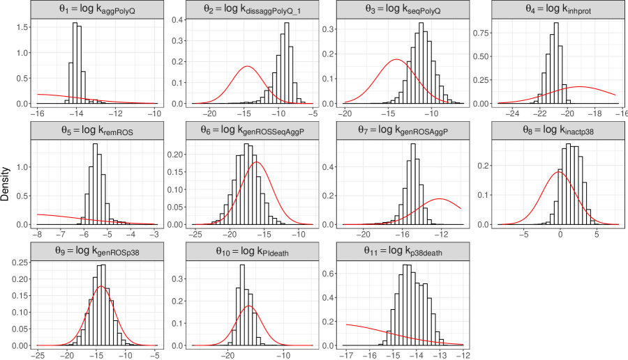
Figure 5: Marginal prior and posterior distributions for the (logged) stochastic kinetic rate parameters (histogram – posterior; red curve – prior).

Graphical summaries of the marginal posterior distributions of the (logged) kinetic rates are given in Figure 5. The figure shows that, despite the experimental data being thought to perhaps give only a very partial insight into the biological mechanism, it has in fact been very informative about many parameters. The analysis has confirmed values, with very much increased precision, for the rates of cell death due to activation of p38 ($k_{p38death}$) and due to inhibition of the proteasome by aggregates ($k_{PIdeath}$), which were also observed but with no information on cause of death. It is of particular note that the posterior distribution suggests that the early stages of the aggregation process, when it is reversible, probably occur at a much faster rate than had previously been assumed. This suggests that both the disaggregation of small aggregates and the formation and early growth of aggregates are more rapid. Also the ratio of disaggregation and aggregation rates $(k_{disaggPolyQ_{1}}/k_{aggPolyQ})$ is around an order of magnitude higher than was thought. This suggests on the one hand that it may take longer to reach the threshold size required for inclusion formation but also that there will be more small aggregates present which will inhibit the proteasome. The decrease in posterior mean also suggests that proteasome inhibition ($k_{inhprot}$) is likely to occur at a slower rate than first thought; probably due to originally underestimating the production of small aggregates.

Looking at the rates involved in ROS turnover, the posterior suggests that the rate at which ROS is removed (kremROS) is faster and that less ROS is generated by small aggregates (kgenROSAggP) than was thought, which means that the generation of ROS via the p38 pathway probably plays a larger contribution. This confirms the suggestion by Tang et al. (2010) that p38 inhibitors, an experimental intervention that they tested, have therapeutic potential to reduce the detrimental effects of the aggregation process.

Figure 6 shows summaries of the marginal posterior distributions of the (logged) measurement error levels.

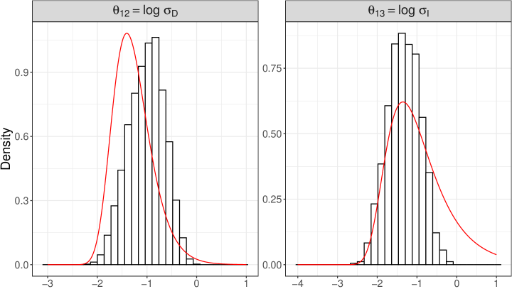
Figure 6: Marginal posterior distributions for the (logged) measurement error parameters (histogram – posterior; red curve – prior).

We have also looked at the overall adequacy of the stochastic and observational models by comparing the observed proportions under the three conditions with their posterior predictive distribution. These distributions can be determined by first running the stochastic model at a sample of realisations from the posterior distribution of the model parameters and then obtaining realisations from the observation model using this output. Figure 7 shows, for each experimental condition, 95% predictive intervals for the proportions of cell death or inclusion bodies on the logit scale, with the experimental data shown as crosses. The positions of the data points in these intervals suggest that there are no obvious departures from the joint observation-biological stochastic model, though there is, of course, scope for model refinement and further experiments.

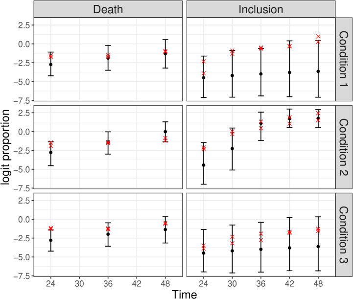
Figure 7: Mean and 95$\%$ posterior predictive intervals for the proportions of cell death and of inclusions for each experimental condition, with the experimental data shown as crosses.

Supplementary Materials

Web Appendix 1 referenced in Sections 3, 7 and 8 is available upon request. The associated computer code is available from

https://github.com/csgillespie/polyglutamine-inference

References

- Bastos and O’Hagan, (2009) Bastos, L. S. and O’Hagan, A. (2009). Diagnostics for Gaussian process emulators. Technometrics, 51:425–438.
- Bayarri et al., (2007) Bayarri, M. J., Berger, J. O., Paulo, R., Sacks, J., Cafeo, J. A., Cavendish, J., Lin, C.-H., and Tu, J. (2007). A framework for validation of computer models. Technometrics, 49:138–154.
- Boys et al., (2008) Boys, R. J., Wilkinson, D. J., and Kirkwood, T. B. L. (2008). Bayesian inference for a discretely observed stochastic kinetic model. Statistics and Computing, 18(2):125–135.
- Cao et al., (2006) Cao, Y., Gillespie, D. T., and Petzold, L. R. (2006). Efficient step size selection for the tau-leaping simulation method. Journal of Chemical Physics, 124:044109.
- Carpenter et al., (2017) Carpenter, B., Gelman, A., Hoffman, M., Lee, D., Goodrich, B., Betancourt, M., Brubaker, M., Guo, J., Li, P., and Riddell, A. (2017). Stan: A probabilistic programming language. Journal of Statistical Software, Articles, 76(1):1–32.
- Cumming and Goldstein, (2010) Cumming, J. A. and Goldstein, M. (2010). Bayes linear uncertainty analysis for oil reservoirs based on multiscale computer experiments. In O’Hagan, A. and West, M., editors, The Oxford Handbook of Applied Bayesian Analysis, pages 241–270. Oxford University Press, Oxford.
- Elowitz et al., (2002) Elowitz, M., Levine, A., Sigga, E., and Swain, P. (2002). Stochastic gene expression in a single cell. Science, 297(5584):1183–1186.
- Gabry, (2018) Gabry, J. (2018). shinystan: Interactive Visual and Numerical Diagnostics and Posterior Analysis for Bayesian Models. R package version 2.5.0.
- Gelman and Rubin, (1992) Gelman, A. and Rubin, D. B. (1992). Inference from iterative simulation using multiple sequences. Statist. Sci., 7(4):457–472.
- Georgoulas et al., (2016) Georgoulas, A., Hillston, J., and Sanguinetti, G. (2016). Unbiased Bayesian inference for population Markov jump processes via random truncations. Statistics and Computing, 27:991–1002.
- Gillespie, (1977) Gillespie, D. T. (1977). Exact stochastic simulation of coupled chemical reactions. Journal of Physical Chemistry, 81:2340–2361.
- Gillespie, (2000) Gillespie, D. T. (2000). The chemical Langevin equation. Journal of Chemical Physics, 113:297–306.
- Gillespie, (2001) Gillespie, D. T. (2001). Approximate accelerated stochastic simulation of chemically reacting systems. Journal of Chemical Physics, 115:1716.
- Gneiting et al., (2007) Gneiting, T., Balabdaoui, F., and Raftery, A. E. (2007). Probabilistic forecasts, calibration and sharpness. Journal of the Royal Statistical Society: Series B (Statistical Methodology), 69:243–268.
- Golightly and Wilkinson, (2011) Golightly, A. and Wilkinson, D. J. (2011). Bayesian parameter inference for stochastic biochemical network models using particle Markov chain Monte Carlo. Interface Focus, 1:807–820.
- Henderson et al., (2009) Henderson, D. A., Boys, R. J., Krishnan, K. J., Lawless, C., and Wilkinson, D. J. (2009). Bayesian emulation and calibration of a stochastic computer model of mitochondrial DNA deletions in substantia nigra neurons. Journal of the American Statistical Association, 104:76–87.
- Henderson et al., (2010) Henderson, D. A., Boys, R. J., Proctor, C. J., and Wilkinson, D. J. (2010). Linking systems biology models to data: a stochastic kinetic model of p53 oscillations. In O’Hagan, A. and West, M., editors, The Oxford Handbook of Applied Bayesian Analysis, pages 155–187. Oxford University Press, Oxford.
- Ibrahim and Chen, (2000) Ibrahim, J. G. and Chen, M.-H. (2000). Power prior distributions for regression models. Statistical Science, 15(1):pp. 46–60.
- Kitano, (2001) Kitano, H. (2001). Foundations of Systems Biology. MIT Press.
- Koblents et al., (2019) Koblents, E., Mariño, I. P., and Míguez, J. (2019). Bayesian computation methods for inference in stochastic kinetic models. Complexity, 2019.
- Koblents and Míguez, (2015) Koblents, E. and Míguez, J. (2015). A population monte carlo scheme with transformed weights and its application to stochastic kinetic models. Statistics and Computing, 25:407–425.
- Morris and Mitchell, (1995) Morris, M. D. and Mitchell, T. J. (1995). Explanatory designs for computational experiments. Journal of Statistical Planning and Inference, 43(3):381–402.
- O’Hagan, (2006) O’Hagan, A. (2006). Bayesian analysis of computer code outputs: a tutorial. Reliability Engineering and System Safety, 91:1290–1300.
- Owen et al., (2015) Owen, J., Wilkinson, D. J., and Gillespie, C. S. (2015). Likelihood free inference for Markov processes: a comparison. Statistical Applications in Genetics and Molecular Biology, 14:189–209.
- Persichetti et al., (1996) Persichetti, F., Carlee, L., Faber, P. W., McNeil, S. M., Ambrose, C. M., Srinidhi, J., Anderson, M., Barnes, G. T., Gusella, J. F., and MacDonald, M. E. (1996). Differential expression of normal and mutant Huntington’s disease gene alleles. Neurobiology of Disease, 3(3):183 – 190.
- Rasmussen and Williams, (2006) Rasmussen, C. E. and Williams, C. K. I. (2006). Gaussian Processes for Machine Learning. MIT Press.
- Santner et al., (2003) Santner, T. J., Williams, B. J., and Notz, W. I. (2003). The Design and Analysis of Computer Experiments. Springer, New York.
- Stan Development Team, (2018) Stan Development Team (2018). RStan: the R interface to Stan. R package version 2.18.2.
- Swain et al., (2002) Swain, P., Elowitz, M., and Siggna, E. (2002). Intrinsic amd extrinsic conributions to stochasticity in gene expression. PNAS, 99(20):12795–12800.
- Tang et al., (2010) Tang, M. Y., Proctor, C. J., Woulfe, J., and Gray, D. A. (2010). Experimental and computational analysis of polyglutamine-mediated cytotoxicity. PLOS Computational Biology, 6(9):1–14.
- van Kampen, (2001) van Kampen, N. G. (2001). Stochastic Processes in Physics and Chemistry. North-Holland.
- Vernon et al., (2014) Vernon, I., Goldstein, M., and Bower, R. (2014). Galaxy formation: Bayesian history matching for the observable universe. Statist. Sci., 29(1):81–90.
- Villaverde and Banga, (2014) Villaverde, A. F. and Banga, J. R. (2014). Reverse engineering and identification in systems biology: strategies, perspectives and challenges. J. R. Soc. Interface, 11:20130505.
- Wilkinson, (2018) Wilkinson, D. J. (2018). Stochastic Modelling for Systems Biology. Chapman & Hall/CRC Mathematical & Computational Biology. Taylor & Francis, 3 edition.
- Wu et al., (2014) Wu, Q., Smith-Miles, K., and Tian, T. (2014). Approximate bayesian computation schemes for parameter inference of discrete stochastic models using simulated likelihood density. BMC Bioinformatics, 15:S3.