Kernel-based $L_{2}$-Boosting with Structure Constraints

Abstract

Developing efficient kernel methods for regression is very popular in the past decade. In this paper, utilizing boosting on kernel-based weaker learners, we propose a novel kernel-based learning algorithm called kernel-based re-scaled boosting with truncation, dubbed as KReBooT. The proposed KReBooT benefits in controlling the structure of estimators and producing sparse estimate, and is near overfitting resistant. We conduct both theoretical analysis and numerical simulations to illustrate the power of KReBooT. Theoretically, we prove that KReBooT can achieve the almost optimal numerical convergence rate for nonlinear approximation. Furthermore, using the recently developed integral operator approach and a variant of Talagrand’s concentration inequality, we provide fast learning rates for KReBooT, which is a new record of boosting-type algorithms. Numerically, we carry out a series of simulations to show the promising performance of KReBooT in terms of its good generalization, near over-fitting resistance and structure constraints.

Keywords: Learning theory, kernel methods, boosting, re-scaling, truncation

1 Introduction

In a regression problem, data of input-output pairs are given to feed the learning with the purpose of modeling the relationship between inputs and outputs. Kernel methods (Evgeniou et al., 2000), which map input points from the input space to some kernel-based feature space to make the learning method be linear, have been widely used for regression in the last two decades. Learning algorithms including kernel ridge regression (Caponnetto and De Vito, 2007), kernel-based gradient descent (Yao et al., 2007), kernel-based spectral algorithms (Gerfo et al., 2008), kernel-based conjugate gradient algorithms (Blanchard and Kr$\ddot{\mbox{a}}$mer, 2016) and kernel-based LASSO (Wang et al., 2007) have been proposed for regression with perfect feasibility verifications. To attack the design flaw of kernel methods in computation, several variants such as distributed learning (Zhang et al., 2015), localized learning (Meister and Steinwart, 2016) and learning with sub-sampling (Grittens and Mahoney, 2016), have been developed to derive scalable kernel-based learning algorithms and been successfully used in numerous massive data regression problems.

Our purpose is not to pursue novel scalable variants of kernel methods to tackle massive data, but to present novel kernel-based learning algorithms to realize different utility of data. This is a hot topic in recent years and numerous novel kernel-based learning algorithms have been proposed for different purpose. In particular, (Lin and Zhou, 2018b) proposed the kernel-based partial least squares to accelerate the convergence rate of kernel-based gradient descent and provided optimal learning rate verifications; (Guo et al., 2017b) developed a kernel-based threshold algorithms to derive sparse estimator to enhance the interpretability and reduce testing time; (Guo et al., 2017c) proposed a bias corrected regularization kernel network to reduce the bias of kernel ridge regression; and more recently (Lin et al., 2019) combined the well known $L_{2}$-Boosting (Bühlmann and Yu, 2003) with kernel ridge regression to avoid the saturation of kernel ridge regression and reduce the difficulty of parameter-selection.

Besides the generalization capability (Evgeniou et al., 2000), three important factors affecting the learning performance of a kernel-based algorithm are the computational complexity, parameter selection and interpretability. The computational complexity (Rudi et al., 2015) reflects the time price of a learning algorithm in a single trail; the parameter selection (Caponnetto and Yao, 2010) frequently refers to the number of trails in the learning process and the interpretability in the framework of kernel learning (Shi et al., 2011) usually concerns the sparseness of the derived estimator. Our basic idea is to combine kernel methods with a new variant of boosting to derive a learning algorithms that is user-friendly, over-fitting resistant and well interpretable. Taking a set of kernel functions as the weak learners, the variant of boosting combines the ideas of regularization in (Zhang and Yu, 2005) and re-scaling in (Wang et al., 2019).

The idea of Regularization aims at controlling the step-size of boosting iterations and derives estimators with structure constraints (relatively small $\ell_{1}$ norm). Regularized boosting via truncation (RTboosting) (Zhang and Yu, 2005) is a typical variant of boosting based on regularization. RTboosting controls the step-size in each boosting iteration via limiting the range of linear search, which succeeds in improving the performance of boosting and enhancing the interpretability. However, to the best of our knowledge, fast numerical convergence rates were not provided for these variants. In particular, it can be found in (Zhang and Yu, 2005) that the numerical convergence of RTboosting is of an order $\mathcal{O}(k^{-1/3})$, which is far worse than the optimal rate for nonlinear approximation $\mathcal{O}(k^{-1})$ (DeVore and Temlaykov, 1996). Here and hereafter, $k$ denotes the number of boosting iterations. The idea of re-scaling focuses on multiplying a re-scaling parameter to the estimator of each boosting iteration to accelerate the numerical convergence rate of boosting. In particular, re-scaled boosting (Rboosting) (Wang et al., 2019) which shrinks the estimator obtained in the previous boosting iteration was shown to achieve the optimal numerical convergence rate under certain sparseness assumption. The problem is, however, there aren’t any guarantees for the structure ($\ell_{1}$ norm) of the estimator, making the strategy lack of interpretability.

In this paper, we propose a novel kernel-based re-scaled boosting with truncation (KReBooT) to embody advantages of regularization and re-scaling simultaneously. We find a close relation between the regularization parameter and re-scaling parameter to accelerate the numerical convergence and control the $\ell_{1}$ norm of the derived estimator. This together with the well developed integral operator technique in (Lin et al., 2017; Guo et al., 2017a) and a Talagrand’s concentration inequality (Steinwart and Christmann, 2008) yields an almost optimal numerical convergence rate and a fast learning rate of KReBooT. In particular, the new algorithm can achieve a learning rate as far as $\mathcal{O}(\frac{1}{m}\log^{2}m)$ under some standard assumptions to the kernel, where $m$ is the number of training samples. Due to the structure constraint again, we also prove that the new algorithm is almost overfitting resistant in the sense that the bias decreases inversely proportional to $k$, while the variance increases logarithmical with respect to $k$. Finally, it should be mentioned that there are totally three types of parameters including re-scaling parameters, regularization parameters and iteration numbers involved in the new algorithm. Our theoretical analysis shows that the learning performance is not sensitive to them, making the algorithm to be user-friendly. In fact, the re-scaling and regularization parameters can be determined before the learning process and the number of iterations can be selected to be relatively large, since KReBooT is almost overfitting resistant. We conduct a series of numerical simulations to illustrate the outperformance of the new algorithm, compared with widely used kernel methods. The numerical results are consistent with our theoretical claims and therefore verify our assertions.

The rest of paper is organized as follows. In the next section, we introduce detailed implementation of KReBooT. Section 3 provides convergence guarantees for KReBooT as well as its almost optimal numerical convergence rate. In Section 4, we derive fast learning rate for KReBooT in the framework of learning theory. Section 5 presents the numerical verifications for our theoretical assertions. In Section 6, we prove our main results.

2 Kernel-based Re-scaled Boosting with Truncation

Let $D=\{z_{i}\}_{i=1}^{m}=\{(x_{i},y_{i})\}_{i=1}^{m}$ be the set of samples with $x_{i}\in\mathcal{X}$ and $y_{i}\in\mathcal{Y}$, where $\mathcal{X}$ is a compact input space and $\mathcal{Y}\subseteq[-M,M]$ is the output space for some $M>0$. Given a Mercer kernel $K:\mathcal{X}\times\mathcal{X}\to\mathbb{R}$, denote by $(\mathcal{H}_{K},\|\cdot\|_{K})$ the corresponding reproducing kernel Hilbert space (RKHS). The compactness of $\mathcal{X}$ implies $\kappa:=\sqrt{\sup_{x\in\mathcal{X}}K(x,x)}\leq\infty$. Throughout this paper, we assume $\kappa\leq 1$ for the sake of brevity. Set $S:=\{K_{x_{i}}:i=1,\dots,m\}$ with $K_{x}(\cdot)=K(\cdot,x)$. Let $\mathcal{H}_{K,D}:=\left\{\sum_{i=1}^{m}a_{i}K_{x_{i}}:a_{i}\in\mathbb{R}\right\}.$ The well known representation theorem (Cucker and Zhou, 2007) shows that all the aforementioned kernel-based algorithms build an estimator in $\mathcal{H}_{K,D}$. Thus, it is naturally to take $\mathcal{H}_{K,D}$ rather than $\mathcal{H}_{K}$ as the hypothesis space.

Kernel-based boosting aims at learning an estimator from $\mathcal{H}_{K,D}$ based on $D$. Using different sets of weak learners, there are two strategies of kernel-based boosting. The one is to employ functions in $\mathcal{H}_{K,D}$ with small RKHS norms as the set of weak learners. Using the standard gradient descent technique, this type of $L_{2}$-Boosting boils down to iterative residual fitting scheme and was proved in (Lin et al., 2019) to be almost over-fitting resistant in the sense that its bias increases exponentially while its variance increases with a exponentially small increment as the boosting iteration happens. However, such a near over-fitting resistance is built upon some minimum eigen-value assumption of the kernel matrix, which is difficult to check for general data distributions and kernels. The other is to use $S$ as the set of weak learners (Zhang and Yu, 2005). This strategy coincides with the well known greedy algorithms (Barron et al., 2008) and dominates in reducing the computational burden and deducing sparse estimator (Zhang and Yu, 2005). However, the learning rate of these algorithms are usually slow, especially, only an order of $m^{-1/2}$ can be guaranteed (Barron et al., 2008).

In this paper, we focus on designing a kernel-based $L_{2}$-Boosting algorithm which is near over-fitting resistant for general kernels and data distributions, user-friendly and theoretically feasible. Our basic idea is to combine the classical truncation operator in (Zhang and Yu, 2005) to reduce the variance and a recently developed re-scaling technique in (Wang et al., 2019) to accelerate the numerical convergence rate. We thus name the new algorithm as kernel-based re-scaled boosting with truncation (KReBooT). Given a set of re-scaling parameters $\{\alpha_{k}\}_{k=1}^{\infty}$ with $\alpha_{k}\in(0,1)$ and a set of non-decreasing step sizes $\{l_{k}\}_{k=1}^{\infty}$. KReBooT starts with $f_{D,0}=0$ and then iteratively runs the following two steps:
Step 1 (Projection of gradient): Find $g_{k}^{*}\in S$ such that

$$g^{*}_{k}:=g^{*}_{k,D}:=\arg{\max_{g\in S}}|{\langle y-f_{D,k-1},g\rangle_{m}}|,$$ (1)

where $\langle f,g\rangle_{m}:=\frac{1}{m}\sum_{i=1}^{m}f(x_{i})g(x_{i})$ and $y$ is a function satisfying $y(x_{i})=y_{i}$.
Step 2 (Line search with re-scaling and truncation): Define

$$f_{D,k}:=(1-\alpha_{k})f_{D,k-1}+\beta_{k}^{*}g^{*}_{k},$$ (2)

where

$$\beta_{k}^{*}:=\arg\min_{\beta\in\Lambda_{k}}\left\|(1-\alpha_{k})f_{D,k-1}+\beta g_{k}^{*}-y\right\|_{m}^{2}$$ (3)

and $\Lambda_{k}:=[-\alpha_{k}l_{k},\alpha_{k}l_{k}].$

Compared with the classical boosting algorithm in which the linear search is on $\mathbb{R}$ rather than $\Lambda_{k}$ and $\alpha_{k}=0$, KReBooT involves two crucial operators, i.e., re-scaling and truncation, to control the structure of the derived estimator. In fact, we can derive the following structure constraint for KReBooT.

Lemma 1

Let $f_{D,k}$ be defined by (2). If $\{l_{k}\}_{k=1}^{\infty}$ with $l_{k}\geq 0$ is nondecreasing, then

$$\|f_{D,k}\|_{\ell_{1}}\leq l_{k},\qquad\forall k=0,1,\dots.$$

Proof  It follows from $\Lambda_{1}=[-\alpha_{1}l_{1},\alpha_{1}l_{1}]$, $\alpha_{1}\leq 1$ and $f_{D,0}=0$ that

$$\|f_{D,1}\|_{\ell_{1}}\leq(1-\alpha_{1})\|f_{D,0}\|_{\ell_{1}}+l_{1}\leq l_{1}.$$

If we assume $\|f_{D,k}\|_{\ell_{1}}\leq l_{k}$, then (2) yields

$$\|f_{D,k+1}\|_{\ell_{1}} \leq (1-\alpha_{k+1})\|f_{D,k}\|_{\ell_{1}}+\alpha_{k+1}l_{k+1}$$

$$\leq (1-\alpha_{k+1})l_{k+1}+\alpha_{k+1}l_{k+1}=l_{k+1}.$$

This proves Lemma 1 by induction.  

Lemma 1 shows that the $\ell_{1}$ norm of the KReBoot estimator can be bounded by the step-size parameter $l_{k}$ via re-scaling and truncation. With this, we can tune $l_{k}$ to control the structure of the estimator and consequently derive a near over-fitting resistent learner. There are totally three types of parameters in the new algorithm: re-scaling parameter $\alpha_{k}$, step-size parameter $l_{k}$ and iteration number $k$. It should be highlighted that $l_{k}$ is imposed to control the structure, $\alpha_{k}$ is adopted to accelerate the numerical convergence rate and $k$ is the number of iteration. We will present detailed parameter-selection strategies after the theoretical analysis.

Although, there are more tunable parameters than the classical boosting algorithm, we will show that the difficulty of selecting each parameter is much less than other variants of boosting (Zhang and Yu, 2005; Xu et al., 2017). Furthermore, the re-scaling and truncation operators do not require additional computation in each boosting iteration. In fact, for arbitrary $g\in S$ and $\beta\in\Lambda_{k}$, we have

$$\left\|[(1-\alpha_{k})f_{D,k-1}+\beta g]-y\right\|_{m}^{2}=\frac{1}{m}\sum_{i=1}^{m}[(1-\alpha_{k})f_{D,k-1}(x_{i})-y_{i}]^{2}+\beta^{2}\frac{1}{m}\sum_{i=1}^{m}g^{2}(x_{i})$$

$$- 2\beta\frac{1}{m}\sum_{i=1}^{m}[(1-\alpha_{k})f_{D,k-1}(x_{i})-y_{i}]g(x_{i}).$$

Direct computation then yields

$$\beta_{k}^{*}:=sign(\langle r_{k-1},g_{k}^{*}\rangle_{m})\min\left\{\frac{\left|\langle r_{k-1},g^{*}_{k}\rangle_{m}\right|}{\|g_{k}^{*}\|_{m}^{2}},\alpha_{k}l_{k}\right\},$$ (4)

where $r_{k-1}:=r_{D,k-1}:=y-(1-\alpha_{k})f_{D,k-1}$ and $sign(\cdot)$ is the sign function. With these, we summary the detailed implementation of KReBooT in Algorithm 1.

  Input: $D=\{(x_{i},y_{i})\}_{i=1}^{m}$, kernel $K(\cdot,\cdot)$.

  Parameters: Re-scaling parameter $\alpha_{k}\in(0,1)$, step size $l_{k}\in\mathbb{R}_{+}$, and number of iterations $k=1,2,\dots,$

  for $k=1,\ldots$ do

     $\blacktriangleright$ (Projection of Gradient) Find $g_{k}^{*}\in S$ satisfying (1).

     $\blacktriangleright$(Line search with re-scaling and truncation) Define

$$f_{D,k}:=(1-\alpha_{k})f_{D,k-1}+\beta_{k}^{*}g^{*}_{k},$$

where $\beta_{k}^{*}$ is obtained by (4) and $f_{D,0}=0$.

  end for

Algorithm 1 KReBooT

3 Numerical Convergence of KReBooT

Lemma 1 presents a structure constraint on the derived estimator of Algorithm 1. In this section, we conduct the numerical convergence analysis for KReBooT. At first, we present a sufficient condition for $\{\alpha_{k}\}_{k=1}^{\infty}$ to guarantee the convergence of Algorithm 1 in the following theorem.

Theorem 2

Assume $|y_{i}|\leq M$ and $\kappa\leq 1.$ Given the non-decreasing sequence $\{l_{k}\}_{k=1}^{\infty}$ and non-increasing $\{\alpha_{k}\}_{k=1}^{\infty}$ with $\alpha_{k}\in(0,1)$, if

$$\lim_{k\rightarrow\infty}\alpha_{k}=0,\qquad\mbox{and}\quad\sum_{k=1}^{\infty}\alpha_{k}=\infty,$$ (5)

then

$$\lim_{k\rightarrow\infty}f_{D,k}=\left\{\begin{array}[]{cc}\arg\min_{f\in\mathcal{H}_{K,D}}\frac{1}{m}\sum_{i=1}^{m}(f(x_{i})-y_{i})^{2},&\mbox{if}\ \lim_{k\rightarrow\infty}l_{k}=\infty,\\ \arg\min_{f\in B_{L}}\frac{1}{m}\sum_{i=1}^{m}(f(x_{i})-y_{i})^{2},&\mbox{if}\ l_{k}=L,\end{array}\right.$$ (6)

where $B_{L}:=\left\{f=\sum_{i=1}^{m}a_{i}K_{x_{i}}:\|f\|_{\ell_{1}}=\sum_{i=1}^{m}|a_{i}|\leq L\right\}$.

Algorithm 1 shows that the range of linear search is $[-\alpha_{k}l_{k},\alpha_{k}l_{k}]$, which means that $\lim_{k\rightarrow\infty}\alpha_{k}=0$ together with not so large $l_{k}$ guarantee the convergence of KReBooT. An extreme case is to set $\alpha_{k}=0$, where the step size is always to be zero and the output is always $f_{D,0}=0$. Under this circumstance, the condition $\sum_{k=1}^{\infty}\alpha_{k}=\infty$ guarantees the effectiveness of the boosting iteration and controls where the algorithm converges. For different $l_{k}$, KReBooT converges either to an empirical kernel-based least-squares solution or a kernel-based LASSO solution. Therefore, KReBooT with $l_{k}=L$ is a feasible and efficient algorithm to solve the kernel-based LASSO, whose learning rates were established in the learning theory community (Shi et al., 2011; Shi, 2013; Guo and Shi, 2013).

Due to the special iteration rule of KReBooT, its numerical convergence rate depends heavily on the re-scaling parameter $\alpha_{k}$. If $\alpha_{k}$ is too large, then the re-scaling operator offsets the effectiveness of the previous boosting iteration, making the numerical convergence rate be slow. On the contrary, if $\alpha_{k}$ is too small, then step sizes of the linear search are also very small, reducing the effectiveness of boosting iterations. Therefore, a suitable selection of the re-scaling parameter $\alpha_{k}$ is highly desired in KReBooT. In the following theorem, we show that, KReBooT with $\alpha_{k}=\frac{2}{k+2}$, can achieve the optimal numerical convergence rate of nonlinear approximation.

Theorem 3

Assume $|y_{i}|\leq M$ and $\kappa\leq 1.$ For arbitrary $h\in\mathcal{H}_{K,D}$ with $\|h\|_{\ell_{1}}<\infty$, if $\alpha_{k}=\frac{2}{k+2}$ and $\{l_{k}\}_{k=1}^{\infty}$ is a sequence of nondecreasing positive numbers satisfying $\lim_{k\rightarrow\infty}l_{k}=\infty$, then

$$\|y-f_{D,k}\|_{m}^{2}-\|y-h\|_{m}^{2}\leq 32\max\left\{16k^{*}_{h}\left[M^{2}(k^{*}_{h}+4)+8l_{k^{*}_{h}}^{2}\right],15\right\}k^{-1},$$ (7)

where $k^{*}_{h}$ is the smallest positive integer satisfying $l_{k^{*}_{h}}\geq\|h\|_{\ell_{1}}.$

In (7), the convergence rate depends on $k^{*}_{h}$ and $l_{k^{*}_{h}}$. For a given $h$ with $\|h\|_{\ell_{1}}<\infty$ and a nondecreasing positive numbers $\{l_{k}\}_{k=1}^{\infty}$ with $\lim_{k\rightarrow\infty}l_{k}=\infty$, there always exists a constant $k^{*}_{h}$ such that $l_{k^{*}_{h}}\geq\|h\|_{\ell_{1}}$. Under this circumstance, $k^{*}_{h}$ and $l_{k^{*}_{h}}$ can be regarded as constants in the estimate. However, it should be mentioned that for $k$ satisfying $l_{k}<\|h\|_{\ell_{1}}$, the boosting iteration in Algorithm 1 is not effective and the algorithm requires increasing property of $\{l_{k}\}_{k=1}^{\infty}$. Once $l_{k}\geq\|h\|_{\ell_{1}}$ for some $k$, then the algorithm converges of an order $\mathcal{O}(1/k)$. In this way, the selection of $l_{k}$ is crucial. We recommend to set $l_{k}=c_{0}\log(k+1)$ for some $c_{0}>0$.

A main problem of the classical $L_{2}$-Boosting algorithm is its low numerical convergence rate. Under the same setting as Theorem 3, it was shown in (Livshits, 2009) that the order of numerical convergence rate of $L_{2}$-Boosting lies in $(k^{-0.3796},k^{-0.364})$, which is much slower than the minimax nonlinear approximation rate (DeVore and Temlaykov, 1996), $\mathcal{O}(k^{-1})$, and leaves a large room to be improved. Furthermore, there lacks structure constraint for the derived boosting estimator, which requires in-stable relationship between generalization performance and boosting iterations. Noticing this, (Zhang and Yu, 2005) proposed RTboosting to control the structure for the derived estimator and then improve the generalization performance. However, the best numerical convergence rate of this variant is $\mathcal{O}(k^{-1/3})$ and the $\ell_{1}$ norm of the estimator satisfies $\|f_{D,k}\|_{\ell_{1}}=\mathcal{O}(k^{1/3})$. Using the re-scaling technique in (Bagirov et al., 2010), (Xu et al., 2017) proved that RBoosting can achieve the optimal numerical convergence rate as order $\mathcal{O}(k^{-1})$. The problem is, however, the $\ell_{1}$ norm of the derived estimator is much larger than $\mathcal{O}(k^{1/3})$, which makes the algorithms be sensitive to the re-scaling parameter and number of iterations. Theorem 3 embodies the advantages of RBoosting in terms of optimal numerical convergence rate and RTboosting by means of providing controllable $\ell_{1}$ norm of the derived estimate.

4 Learning Rate Analysis

In this section, we are interested in deriving fast learning rates for KReBooT. Our analysis is carried out in the framework of statistical learning theory (Cucker and Zhou, 2007) , where $D=\{z_{i}\}_{i=1}^{m}=\{(x_{i},y_{i})\}_{i=1}^{m}\subset\mathcal{Z}$ are assumed to be drawn independently according to an unknown joint distribution $\rho:=\rho(x,y)=\rho_{X}(x)\rho(y|x)$ with $\rho_{X}$ the marginal distribution and $\rho(y|x)$ the conditional distribution. The learning performance of an estimator $f$ is measured by the generalization error $\mathcal{E}(f):=\int_{\mathcal{Z}}(f(x)-y)^{2}d\rho.$ Noting that the regression function defined by $f_{\rho}(x)=E[y|X=x]$ minimizes the generalization error, our target is then to learn a function $f_{D}$ to approximate $f_{\rho}$ such that

$$\mathcal{E}(f_{D})-\mathcal{E}(f_{\rho})=\|f_{D}-f_{\rho}\|^{2}_{\rho}$$ (8)

is as small as possible.

To quantify the learning performance of KReBooT, some priori information including the regularity of the regression function and capacity of the assumption space should be given at first. Define $L_{K}:L_{\rho_{X}}^{2}\rightarrow L_{\rho_{X}}^{2}$ (or $\mathcal{H}_{K}\rightarrow\mathcal{H}_{K}$) as

$$L_{K}f:=\int_{\mathcal{X}}K_{x}f(x)d\rho_{X}.$$ (9)

Since $K$ is positive-definite, $L_{K}$ is a positive operator. The following two assumptions describe the regularity of $f_{\rho}$ and capacity of $\mathcal{H}_{K}$, respectively.

Assumption 1

There exists an $h_{\rho}\in L_{\rho_{X}}^{2}$ such that

$$f_{\rho}=L_{K}h_{\rho}=\int_{\mathcal{X}}K_{x}h_{\rho}(x)d\rho_{X}.$$ (10)

Assumption 1 describes the regularity of the regression function and is a bit stronger than the standard assumption $f_{\rho}\in\mathcal{H}_{K}$, i.e. $f_{\rho}=L_{K}^{1/2}h_{\rho}$. Such an assumption is to guarantee that there exists an $f_{0}\in\mathcal{H}_{D,K}$ which approximates $f_{\rho}$ well with high probability and satisfies $\|f_{0}\|_{\ell_{1}}\leq C$ for some constant $C$ depending only on $h_{\rho}$ (See Lemma 10 below). The aforementioned property is standard for boosting algorithms (DeVore and Temlaykov, 1996; Zhang and Yu, 2005; Temlyakov, 2008; Barron et al., 2008; Mukherjee et al., 2013; Temlyakov, 2015; Petrova, 2016; Xu et al., 2017; Wang et al., 2019). The second assumption concerns the eigenvalue-decay associated with $L_{K}$.

Assumption 2

Let $\{(\mu_{\ell},\phi_{\ell})\}_{\ell=1}^{\infty}$ be a set of normalized eigenpairs of $L_{K}$ with $\{\mu_{\ell}\}_{\ell=1}^{\infty}$ arranging in a non-increasing order. For $0<s<1$ and some $c>0$, we assume

$$\mu_{\ell}\leq c\ell^{-1/s},\qquad\forall\ell\geq 1.$$ (11)

The above assumption depicts the capacity of $\mathcal{H}_{K}$ as well as $\mathcal{H}_{K,D}$. Since the estimator derived by Algorithm 1 under Assumption 1 is always in $\mathcal{H}_{K,D}$ with structure constraints, its generalization performance depends heavily on the kernel and consequently $s$ in Assumption 2. Assumption 2 is slight stronger than the effective dimension assumption in (Guo et al., 2017a; Lin et al., 2017; Lu et al., 2018) and is widely used in bounding learning rates for numerous kernel approaches (Caponnetto and De Vito, 2007; Steinwart et al., 2009; Raskutti et al., 2014; Zhang et al., 2015; Lin et al., 2019). By the help of the above two assumptions, we present our third main result in the following theorem, which quantifies the learning performance of KReBooT.

Theorem 4

Let $0<\delta<1$ and $f_{D,k}$ be defined by (2) with $\alpha_{k}=\frac{2}{k+2}$ and $l_{k}=c_{0}\log(k+1)$ for some $c_{0}>0$. Under Assumption 1 and Assumption 2 with some $0<s<1$ and $c>0$, if $|y_{i}|\leq M$, $\kappa\leq 1$ and $m^{-1/(s+1)}\log^{2}\frac{6}{\delta}\leq 1$, then for arbitrary $k\geq c_{1}m^{\frac{1}{1+s}}$ with confidence $1-\delta$, there holds

$$\mathcal{E}(f_{D,k})-\mathcal{E}(f_{\rho})\leq C\left(\log(k+1)\right)^{2}m^{-\frac{1}{1+s}}\log^{4}\frac{18}{\delta},$$ (12)

where $c_{1}$ and $C$ are constants independent of $m$, $k$ or $\delta$.

Theorem 4 shows that for $k=m$ and sufficiently small $s$, KReBooT achieves a learning rate of order $\mathcal{O}(m^{-1}(\log m)^{2})$. It should be mentioned that it is a new record for boosting-type algorithms. In particular, under the similar setting as this paper, the learning rate of RTboosting (Zhang and Yu, 2005) is slower than $\mathcal{O}(m^{-1/2})$ while it of Rboosting (Barron et al., 2008) is $\mathcal{O}(m^{-1/2})$. However, the derived learning rate in Theorem 4 is slower than some existing kernel approaches like kernel ridge regression (Lin et al., 2017), kernel gradient descent (Lin and Zhou, 2018a), kernel partial least squares (Lin and Zhou, 2018b), kernel conjugate descent (Blanchard and Kr$\ddot{\mbox{a}}$mer, 2016) and kernel spectral algorithms (Guo et al., 2017a). The reason is that we impose the structure restrictions on the derived estimator as in Lemma 1 to reduce the testing time, enhance the interpretability and maintain the near overfitting resistant property of the algorithm. Under the similar structure constraints, our derived learning rate is much faster than that of kernel-based LASSO (Shi et al., 2011; Shi, 2013; Guo and Shi, 2013).

To guarantee the good learning performance of KReBooT, there are two requirements on the number of iterations, i.e., $k\geq c_{1}m^{1/(1+s)}$ and $k$ is not exponential with respect to $m$. Noting Theorem 3, the former is necessary to derive an estimator of bias $m^{-1/(1+s)}$. The latter, benefiting from the structure constraint of KReBooT, shows its near over-fitting resistance, which is novel for kernel-based learning algorithms and essentially different from the results in (Lin et al., 2019), since we do not impose any lower bounds for eigenvalues of $L_{K}$. This property shows that if $k$ is larger than a specific value of order $m^{1/(1+s)}$, then running KReBooT does not bring essentially negative effect.

Noting that there are three tunable parameters in Algorithm 1, that is, $\alpha_{k}$, $l_{k}$ and $k$. Our theoretical analysis and experimental verification below show that KReBooT is stable with respect to $\alpha_{k}$ and it can be fixed to be $\frac{2}{k+2}$ before the learning process. Moreover, we can set $l_{k}=c_{0}\log(k+1)$ to guarantee the good structure of the KReBooT estimator. Here, $c_{0}$ is a parameter which affects the constant $C$ in (12). In practice, it is somewhat important and should be specified by using some parameter-selection strategies such as “hold-out” (Caponnetto and Yao, 2010) or cross-validation (Györfy et al., 2002). The selection of $k$ depends on $c_{0}$. If $c_{0}$ is extremely large, $\infty$ for example, then the truncation operator does not make sense and the performance of algorithm is sensitive to $k$. If $c_{0}$ is suitable, it follows from Theorem 4 that a large $k$, comparable with $m$ or larger, is good enough. Thus, in the practical implementation of KReBooT, we suggest to set $\alpha_{k}=\frac{2}{k+2}$, $k$ to be large and $l_{k}=c_{0}\log(k+1)$ with $c_{0}$ to be a tunable parameter. Under this circumstance, there is only one key parameter in the new algorithm, which is fewer than other variants of regularized boosting algorithms such as RTboosting and Rboosting.

5 Experiments

In this section, we shall conduct several simulations to verify the merits of the proposed boosting algorithm. In all the simulations, we consider the following regression model:

$$y_{i}=g(x_{i})+\varepsilon_{i},\quad i=1,2,\cdots,N,$$ (13)

where $\varepsilon_{i}$ is the independent Gaussian noise, and

$$g(x):=h_{2}(\|x\|_{2}):=\left\{\begin{array}[]{cc}(1-\|x\|_{2})^{6}(35\|x\|_{2}^{2}+18\|x\|_{2}+3),&0<\|x\|_{2}\leq 1,x\in\mathbb{R}^{3},\\ 0,&\|x\|_{2}>1.\end{array}\right.$$

The kernel used for the proposed KReBooT is chosen as $K(x,x^{\prime})=h_{3}(\|x-x^{\prime}\|_{2})$ with

$$h_{3}(\|x\|_{2}):=\left\{\begin{array}[]{cc}(1-\|x\|_{2})^{4}(4\|x\|_{2}^{2}+1),&0<\|x\|_{2}\leq 1,x\in\mathbb{R}^{3},\\ 0,&\|x\|_{2}>1.\end{array}\right.$$

The reason why we make such choices of $g(\cdot)$ and $K(\cdot)$ is to guarantee Assumption 1 (Chang et al., 2017).

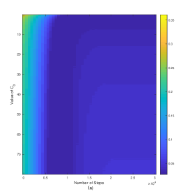
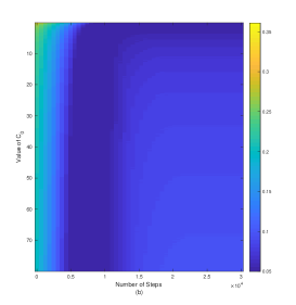
Figure 1: The visualization of testing MSE of the proposed algorithm with varying the number of iterations $k$ and the values of $c_{0}$. (a) $\varepsilon_{i}\sim\mathcal{N}(0,1)$; (b) $\varepsilon_{i}\sim\mathcal{N}(0,2)$.

Simulation I. Besides the number of iterations, there are two additional parameters, the re-scaling parameter $\alpha_{k}$ and the step-size parameter $l_{k}$, may play important roles on the learning performance of KReBooT. According to our theoretical assertions, if $\alpha_{k}=\frac{2}{k+2}$ and $l_{k}\sim c_{0}\log(k+1)$ for some $c_{0}>0$, then KReBooT can attain a fast learning rate. Thus, this simulation mainly focuses on investigating the effect of the constant $c_{0}$ on the prediction performance of KReBooT. To this end, we generate $m=500$ samples for training and $m^{\prime}=500$ samples for testing, under two noise levels, i.e. $\varepsilon_{i}$ is i.i.d. drawn from either $\mathcal{N}(0,1)$ or $\mathcal{N}(0,2)$. We then consider 50 candidates of $c_{0}$ that logarithmical equally spaced in $[0.1,80]$.

Figure 1 gives the visualization of testing mean-squared errors (MSE) of KReBooT with $\alpha_{k}=\frac{2}{k+2}$ via varying the number of iterations $k$ and the value of $c_{0}$. For any fixed step of iteration and $c_{0}$, the testing MSE is the average result over 20 independent trails. It is easy to observe from this figure that, there exits a number of $c_{0}$’s in $[0.1,10]$ for relatively small noise case or in $[0.1,5]$ for relatively large noise case, such that the testing MSE attains a stable value, neglecting the increasing of iterations. This finding means that an appropriate choice of $c_{0}$ could avoid over-fitting. Therefore, for simplicity, we fix $c_{0}=0.5$ in the following simulations.

Simulation II. The objective of this simulation is to describe the relation between the prediction accuracy and the size of training samples for the proposed KReBooT. We thus generate $m=300,900,1500,4500,12000$ samples, respectively, for training, and $m^{\prime}=500$ samples for testing. Similar to the previous simulation, we also consider two noise levels.

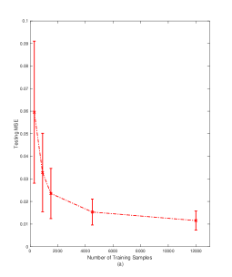
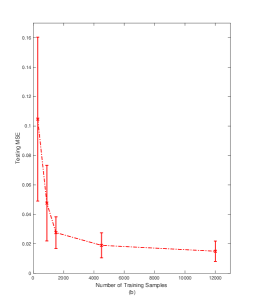
Figure 2: The testing MSE versus the different sizes of training samples. (a) $\varepsilon_{i}\sim\mathcal{N}(0,1)$; (b) $\varepsilon_{i}\sim\mathcal{N}(0,2)$.

Figure 2 depicts the average results over 100 independent trials. It is not hard to observe from this figure that the testing MSE deceases as the number of training samples increases in two noise levels. This partially supports the assertion presented in Theorem 4.

Simulation III. In this simulation, we shall compare the prediction performance of the proposed KReBooT with some other kernel-based methods, including kernel Lasso (Klasso) (Wang et al., 2007), kernel ridge regression (KRR) (Caponnetto and De Vito, 2007), and three kernel version of popular boosting algorithms, i.e., $\epsilon$-boosting (Hastie et al., 2007), rescale-boosting (Wang et al., 2019), regularized boosting with truncation (Zhang and Yu, 2005). We refer to these three kernel-based boosting algorithms as $\epsilon$-Kboosting, KRboosting and KRTboosting, respectively. For two different noise levels, we firstly generate $m=300$ or $1000$ samples to built up the training set, and then generate a validation set of size 500 for tuning the parameters of different methods, and another 500 samples to evaluate the performances in terms of MSE.

Table 1 documents the average MSE over 100 independent runs. Numbers in parentheses are the standard errors. It is not hard to see that the performance of the proposed KReBooT is comparable with Klasso and KRboosting, and clearly better than others. Two important things should be further emphasized. Firstly, though KRboosting illustrates a similar good generalization capability as KReBooT, this algorithm is more likely to overfit, just as the following simulation shown. Secondly, Klasso requires much more time in the training process than the proposed KReBooT.

Table 1: Prediction Performance of Different Methods under Different Settings

Training Size	Noise Level	Methods
			KReBooT	KRboosting	KRTboosting	$\epsilon$-Kboosting	Klasso	KRR
$m=300$	$\sigma^{2}=1$		$0.066\pm 0.036$	$0.064\pm 0.036$	$0.075\pm 0.037$	$0.074\pm 0.036$	$0.065\pm 0.036$	$0.102\pm 0.036$
	$\sigma^{2}=2$		$0.086\pm 0.049$	$0.086\pm 0.047$	$0.101\pm 0.048$	$0.100\pm 0.049$	$0.088\pm 0.048$	$0.137\pm 0.047$
$m=1000$	$\sigma^{2}=1$		$0.027\pm 0.013$	$0.025\pm 0.011$	$0.030\pm 0.010$	$0.029\pm 0.010$	$0.025\pm 0.009$	$0.043\pm 0.013$
	$\sigma^{2}=2$		$0.041\pm 0.021$	$0.039\pm 0.019$	$0.049\pm 0.022$	$0.049\pm 0.023$	$0.040\pm 0.019$	$0.072\pm 0.026$

Simulation IV. In this simulation, we shall show the overfitting resistence of KReBooT, as compared with its two cousins, i.e., KRboosting and KRTboosting. Here we generate 500 samples for training, and another 500 samples for testing, with $\varepsilon_{i}$ is i.i.d. drawn from $\mathcal{N}(0,1)$. Figure 3(a) clearly demonstrates the merits of our proposed KReBooT, that is, the obtained testing MSE does’t increase as the number of iterations increases. In addition, different from KRboosting and KRTboosting, the $\ell_{1}$ norm of the coefficients obtained by KReBooT could converge to a fixed value as shown in Figure 3(b), which conforms to the assertion of structure constraints of KReBoot, just as Lemma 1 purports to show.

Simulation V. In this simulation, we mainly show the coefficients estimation behavior of KReBooT. Similar to the above simulation, KRboosting and KRTboosting are considered for comparison. The aim now is to show the reason why KReBooT is overfitting-resistant. Thus, we generate 500 samples for training, and another 500 samples for testing, under two different noise levels, that is, $\varepsilon_{i}$ is iid drawn from $\mathcal{N}(0,1)$ and $\mathcal{N}(0,2)$. Figures 4 exhibits the numerical results. It can be found in both cases that the $\ell_{1}$ norm of the KReBooT estimator increases much slower than that of other algorithms, which implies that the variance of KReBooT keeps almost the same and is much smaller than other algorithms when the iterations increases. Thus, the generalization error does not increase very much as the iteration happens.

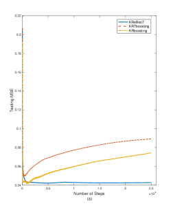
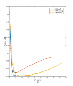
Figure 3: The prediction results obtained by three different kernel-based boosting algorithms. (a) The testing MSE versus the number of steps; (b) The testing MSE versus the $\ell_{1}$ norm.

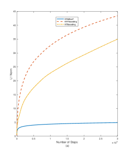
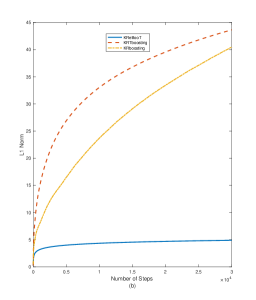
Figure 4: The coefficients estimated by three different kernel-based boosting algorithms versus the number of steps. (a) $\varepsilon_{i}\sim\mathcal{N}(0,1)$; (b) $\varepsilon_{i}\sim\mathcal{N}(0,2)$.

6 Proofs

6.1 Proof of Theorem 2

Before presenting the proof of Theorem 2, we at first proving the following lemma, which shows the role of iterations in kernel-based $L_{2}$-Boosting.

Lemma 5

Let $\Lambda_{k}:=[-\alpha_{k}l_{k},\alpha_{k}l_{k}]$. For arbitrary $h\in\mathcal{H}_{K,D}$ with $\|h\|_{\ell_{1}}<\infty$, if $|y_{i}|\leq M$, $\kappa\leq 1$ and $\{l_{k}\}$ is non-decreasing, then

$$\|y-f_{D,k}\|_{m}^{2}-\|y-h\|^{2}_{m}\leq(1-\alpha_{k})(\|y-f_{D,k-1}\|_{m}^{2}-\|y-h\|^{2}_{m})+2\alpha_{k}^{2}(M+\|h\|_{\ell_{1}})^{2}$$ (14)

holds for all $k\geq k^{*}_{h}:=\arg\min_{k}\{l_{k}\geq\|h\|_{\ell_{1}}\}$.

Proof  For $h\in\mathcal{H}_{K,D}$, write $h=\sum_{i=1}^{m}a_{i,h}K_{x_{i}}$ and $\|h\|_{\ell_{1}}=\sum_{i=1}^{m}|a_{i,h}|$. Define $S^{*}=\{\pm K_{x_{i}}:i=1,\dots,m\}$, then $h=\sum_{i=1}^{m}|a_{i,h}|sign(a_{i,h})K_{x_{i}}$. For $k\geq k^{*}_{h}$, set $\beta=\alpha_{k}\|h\|_{\ell_{1}}$ and notice $\beta\in\Lambda_{k}$. We get from (3) that

$$\|y-f_{D,k}\|_{m}^{2}\leq\|y-(1-\alpha_{k})f_{D,{k-1}}-\beta g_{k}^{*}\|_{m}^{2}=\|(1-\alpha_{k})(y-f_{D,{k-1}})+\alpha_{k}y-\beta g_{k}^{*}\|_{m}^{2}.$$

Since $|y|\leq M$, $|g_{i}|\leq\kappa\leq 1$ and $\beta=\alpha_{k}\|h\|_{\ell_{1}}$, we have

$$\|(1-\alpha_{k})(y-f_{D,{k-1}})+\alpha_{k}y-\beta g_{k}^{*}\|_{m}^{2}$$

$$+ \|(1-\alpha_{k})(y-f_{D,{k-1}})-\alpha_{k}y+\beta g_{k}^{*}\|_{m}^{2}$$

$$= 2(1-\alpha_{k})^{2}\|y-f_{D,{k-1}}\|_{m}^{2}+2\|\alpha_{k}y-\beta g_{k}^{*}\|_{m}^{2}$$

$$\leq 2(1-\alpha_{k})^{2}\|y-f_{D,{k-1}}\|_{m}^{2}+2\alpha_{k}^{2}(M+\|h\|_{\ell_{1}})^{2}.$$

But (1) implies that for arbitrary $g\in S^{*}$,

$$\|(1-\alpha_{k})(y-f_{D,{k-1}})-\alpha_{k}y+\beta g_{k}^{*}\|_{m}^{2}$$

$$\geq (1-\alpha_{k})^{2}\|y-f_{D,{k-1}}\|_{m}^{2}-2\langle(1-\alpha_{k})(y-f_{D,{k-1}}),\alpha_{k}y-\beta g_{k}^{*}\rangle_{m}$$

$$\geq (1-\alpha_{k})^{2}\|y-f_{D,{k-1}}\|_{m}^{2}-2\langle(1-\alpha_{k})(y-f_{D,{k-1}}),\alpha_{k}y-\beta g\rangle_{m}.$$

Then,

$$\|(1-\alpha_{k})(y-f_{D,{k-1}})+\alpha_{k}y-\beta g_{k}^{*}\|_{m}^{2}$$

$$\leq 2(1-\alpha_{k})^{2}\|y-f_{D,{k-1}}\|_{m}^{2}+2\alpha_{k}^{2}(M+\|h\|_{\ell_{1}})^{2}$$

$$- (1-\alpha_{k})^{2}\|y-f_{D,{k-1}}\|_{m}^{2}+2\langle(1-\alpha_{k})(y-f_{D,{k-1}}),\alpha_{k}y-\beta g\rangle_{m}.$$

Since the above estimate holds for arbitrary $g_{i}\in S^{*}$, $i=1,\dots,m$, it also holds for arbitrary convex combination of $\{\pm K_{x_{1}},\dots,\pm K_{x_{m}}\}$. In other words, the above estimate holds for $\sum_{i=1}^{m}b_{i}sign(a_{i,h})K_{x_{i}}$ with $b_{i}\geq 0$ and $\sum_{i=1}^{m}b_{i}=1$. Setting $b_{i}=\frac{a_{i,h}sign(a_{i,h})}{\sum_{i=1}^{m}|a_{i,h}|}$, it follows from $\beta=\alpha_{k}\|h\|_{\ell_{1}}=\alpha_{k}\sum_{i=1}^{m}|a_{i,h}|$ that for $k\geq k^{*}_{h}$,

$$\|y-f_{D,k}\|_{m}^{2}\leq\|(1-\alpha_{k})(y-f_{D,{k-1}})+\alpha_{k}y-\beta g_{k}^{*}\|_{m}^{2}$$

$$\leq (1-\alpha_{k})^{2}\|y-f_{D,{k-1}}\|_{m}^{2}+2\alpha_{k}^{2}(M+\|h\|_{\ell_{1}})^{2}$$

$$+ 2\alpha_{k}\langle(1-\alpha_{k})(y-f_{D,{k-1}}),y-h\rangle_{m}$$

$$\leq (1-\alpha_{k})^{2}\|y-f_{D,{k-1}}\|_{m}^{2}+2\alpha_{k}^{2}(M+\|h\|_{\ell_{1}})^{2}$$

$$+ \alpha_{k}(1-\alpha_{k})\|y-f_{D,{k-1}}\|_{m}^{2}+\alpha_{k}\|y-h\|_{m}^{2}$$

$$= (1-\alpha_{k})\|y-f_{D,{k-1}}\|_{m}^{2}+\alpha_{k}\|y-h\|_{m}^{2}+2\alpha_{k}^{2}(M+\|h\|_{\ell_{1}})^{2}.$$

Hence

$$\|y-f_{D,k}\|_{m}^{2}-\|y-h\|_{m}^{2}\leq(1-\alpha_{k})(\|y-f_{D,k-1}\|_{m}^{2}-\|y-h\|^{2}_{m})+2\alpha_{k}^{2}(M+\|h\|_{\ell_{1}})^{2}.$$

This completes the proof of Lemma 5.  

With the help of the above lemmas, we are in a position to prove Theorem 2.

Proof of Theorem 2. We firs prove (6), which will be divided into the following two steps.

Step 1: Limit inferior. Let $h_{\infty}:=\arg\min_{f\in\mathcal{H}_{K,D}}\frac{1}{m}\sum_{i=1}^{m}(f(x_{i})-y_{i})^{2}.$ It follows from the positive-definiteness of $K$ that there is a set of real numbers $\{a_{i,\infty}\}_{i=1}^{m}$ satisfying $\|h_{\infty}\|_{\ell_{1}}=\sum_{i=1}^{m}|a_{i,\infty}|<\infty$ such that $h_{\infty}=\sum_{i=1}^{m}a_{i,\infty}K_{x_{i}}$. Set $k^{*}_{\infty}:=\arg\min_{k}\{l_{k}\geq\|h_{\infty}\|_{\ell_{1}}\}.$ Then it follows from Lemma 5 that for all $k\geq k^{*}_{\infty}$, there holds

$$\|y-f_{D,k}\|_{m}^{2}-\|y-h_{\infty}\|^{2}_{m}\leq(1-\alpha_{k})(\|y-f_{D,k-1}\|_{m}^{2}-\|y-h_{\infty}\|^{2}_{m})+2\alpha_{k}^{2}(M+\|h_{\infty}\|_{\ell_{1}})^{2}.$$ (15)

We then use (15) to prove

$${\lim\inf}_{k\rightarrow\infty}\|y-f_{D,k}\|_{m}^{2}=\|y-h_{\infty}\|^{2}_{m}$$ (16)

by contradiction. Denote $A_{\infty,k}:=\|y-f_{D,k}\|_{m}^{2}-\|y-h_{\infty}\|^{2}_{m}$. If (16) does not hold, then there exist $K_{\infty}\in\mathbb{N}$ and $\gamma_{\infty}>0$ such that $A_{\infty,k}\geq\gamma_{\infty}$ holds for all $k\geq K_{\infty}$. Since $\alpha_{k}\rightarrow 0$, there exists a $K_{\infty}^{*}\in\mathbb{N}$ such that $\alpha_{k}(M^{2}+\|h_{\infty}\|_{\ell_{1}})\frac{2}{\gamma_{\infty}}\leq\frac{1}{2}$ for all $k\geq K_{\infty}^{*}$. Hence, it follows from (15) that for arbitrary $k>\max\{K_{\infty},K_{\infty}^{*},k^{*}_{\infty}\}$,

$$A_{\infty,k}\leq(1-\alpha_{k})A_{\infty,k-1}+2\alpha_{k}^{2}(M+\|h_{\infty}\|_{\ell_{1}})^{2}$$

$$\leq A_{\infty,k-1}\left[1-\alpha_{k}+\alpha_{k}^{2}(M+\|h_{\infty}\|_{\ell_{1}})^{2}\frac{2}{\gamma_{\infty}}\right]\leq A_{\infty,k-1}(1-\alpha_{k}/2).$$

This together with the assumption $\sum_{k=1}^{\infty}\alpha_{k}=\infty$ yields $A_{\infty,k}\rightarrow 0$ as $k\rightarrow\infty$. Thus, the assumption $\gamma_{\infty}>0$ is false and (16) holds.

Step 2: Limit superior. We then aim at deriving

$${\lim\sup}_{k\rightarrow\infty}\|y-f_{D,k}\|_{m}^{2}=\|y-h_{\infty}\|^{2}_{m}.$$ (17)

For arbitrary $\nu>0$ and $k\geq k^{*}_{\infty}$, Lemma 5 implies

$$A_{\infty,k}-\nu\leq(1-\alpha_{k})(A_{\infty,k-1}-\nu)+2\alpha_{k}^{2}(M+\|h_{\infty}\|_{\ell_{1}})^{2}.$$ (18)

Define $B_{\infty,k}:=A_{\infty,k}-\nu$ and

$$U_{\infty}:=\{k:k\geq k^{*}_{\infty},2\alpha_{k}(M+\|h_{\infty}\|_{\ell_{1}})^{2}\leq B_{\infty,k-1}\}.$$

If $U_{\infty}$ is the finite or empty set, then it follows from $\alpha_{k}\rightarrow 0$ that

$${\lim\sup}_{k\rightarrow\infty}B_{\infty,k-1}\leq 2(M+\|h_{\infty}\|_{\ell_{1}})^{2}\lim_{k\rightarrow\infty}\alpha_{k}=0.$$

This implies

$${\lim\sup}_{k\rightarrow\infty}A_{\infty,k}\leq\nu.$$ (19)

If $U_{\infty}$ is infinite, we have from (18) that

$$B_{\infty,k}\leq\left\{\begin{array}[]{cc}2\alpha_{k}^{2}(M+\|h_{\infty}\|_{\ell_{1}})^{2},&B_{\infty,k-1}=0\\ B_{\infty,k-1}\left(1-\alpha_{k}+2\alpha_{k}^{2}\frac{(M+\|h_{\infty}\|_{\ell_{1}})^{2}}{B_{\infty,k-1}}\right),&B_{\infty,k-1}\neq 0,\end{array}\right.$$ (20)

which implies

$$B_{\infty,k}\leq\max\{2\alpha_{k}^{2}(M+\|h_{\infty}\|_{\ell_{1}})^{2},B_{\infty,k-1}\},\qquad\forall\ k\in U_{\infty}.$$ (21)

Furthermore, (16) shows that there is a subsequence $\{k_{j}\}$ such that $B_{\infty,{k_{j}}}\leq 0$, $j=1,\dots.$ This means

$$U_{\infty}=\bigcup_{j=k_{\infty}^{*}}^{\infty}[m_{j},n_{j}]$$

for some $\{n_{j}\},\{m_{j}\}\subset\mathbb{N}$ satisfying $n_{j-1}<m_{j}-1.$ For $k\notin U_{\infty}$ and $k\geq k_{\infty}^{*}$, we have

$$B_{\infty,k-1}<2\alpha_{k}(M+\|h_{\infty}\|_{\ell_{1}})^{2}.$$ (22)

For $k\in[m_{j},n_{j}]$, it follows from $\alpha_{k+1}\leq\alpha_{k}$, (21), (20) and (22) that

$$B_{\infty,k}\leq\max\{2\alpha_{m_{j}-1}^{2}(M+\|h_{\infty}\|_{\ell_{1}})^{2},B_{\infty,m_{j-1}}\}$$ (23)

$$\leq \max\{2\alpha^{2}_{m_{j}-1}(M+\|h_{\infty}\|_{\ell_{1}})^{2},(1-\alpha_{m_{j}-1})B_{\infty,m_{j-2}}+2\alpha^{2}_{m_{j}-1}(M+\|h_{\infty}\|_{\ell_{1}})^{2}\}$$

$$\leq (1-\alpha_{m_{j}-1})2\alpha_{m_{j}-1}(M+\|h_{\infty}\|_{\ell_{1}})^{2}+2\alpha^{2}_{m_{j}-1}(M+\|h_{\infty}\|_{\ell_{1}})^{2}$$

$$\leq 2\alpha_{m_{j}-1}(M+\|h_{\infty}\|_{\ell_{1}})^{2}.$$ (24)

Combining (22) with (23), we get

$$\lim\sup_{k\rightarrow\infty}B_{\infty,k}\leq 0,$$

which implies

$$\lim\sup_{k\rightarrow\infty}A_{\infty,k}\leq\nu.$$

Since $\nu$ is arbitrary, (17) holds. Thus, (16) and (17) yield (6) by taking the uniqueness of the solution to

$${\arg\min}_{f\in\mathcal{H}_{K,D}}\frac{1}{m}\sum_{i=1}^{m}(f(x_{i})-y_{i})^{2}.$$

If $h\in B_{L}$, it follows from Lemma 5 that (14) holds for all $k\in\mathbb{N}$. Then the same approach as above and Lemma 1 implies (6). This completes the proof of Theorem 2.  

6.2 Proof of Theorem 3

To prove Theorem 3, we need the following lemma.

Lemma 6

Let $j_{0}>2$ be a natural number, $c_{1}<c_{2}\leq j_{0}$ and $\mathcal{C}_{0}(\cdot)$ is a nondecreasing function defined on $\mathbb{R}_{+}$. If $\{a_{v}\}_{v=1}^{\infty}$ satisfies

$$\left\{\begin{array}[]{cc}a_{v}\leq\mathcal{C}_{0}(v)v^{-c_{1}},&1\leq v\leq j_{0},\\ a_{v}\leq a_{v-1}+\mathcal{C}_{0}(v-1)(v-1)^{-c_{1}},&v>j_{0}\end{array}\right.$$ (25)

and

$$a_{v}>\mathcal{C}_{0}(v){v}^{-c_{1}}\quad\mbox{implies}\quad a_{v+1}\leq a_{v}(1-c_{2}/{v}),\qquad\forall v>j_{0},$$ (26)

then there holds

$$a_{k}\leq 2^{\frac{c_{1}c_{2}+c_{2}}{c_{2}-c_{1}}}\mathcal{C}_{0}(k)k^{-c_{1}},\qquad\forall k=1,2,\dots.$$

Proof  For $1\leq v\leq j_{0}$, (25) shows

$$a_{v}\leq\mathcal{C}_{0}(v)v^{-c_{1}}.$$

Thus,

$$V=\{v\in\mathbb{N}:a_{v}>\mathcal{C}_{0}(v)v^{-c_{1}}\}$$

does not contain $1,2,\dots,j_{0}$. Let $v\geq j_{0}+1$ satisfy $v-1\notin V$ and $v\in V$, and $\eta$ be the largest positive integer such that $[v,v+\eta]\subset V$. Then it follows from the non-decreasing of $\mathcal{C}_{0}(\cdot)$ that

$$a_{v-1}\leq\mathcal{C}_{0}(v-1)(v-1)^{-c_{1}}\leq\mathcal{C}_{0}(v)(v-1)^{-c_{1}},$$ (27)

$$a_{v+j}>\mathcal{C}_{0}(v+j)(v+j)^{-c_{1}}\geq\mathcal{C}_{0}(v)(v+j)^{-c_{1}},\qquad\forall j=0,1,\dots,\eta.$$ (28)

Hence, it follows from (26) and (25) that

$$a_{v+\mu}\leq a_{v}\Pi_{u=v}^{v+\mu-1}(1-c_{2}/u)\leq(a_{v-1}+\mathcal{C}_{0}(v-1)(v-1)^{-c_{1}})\Pi_{u=v}^{v+\mu-1}(1-c_{2}/u).$$ (29)

Inserting (28) into the above estimate and noting (27), the nondecreasing of $\mathcal{C}_{0}(\cdot)$ implies

$$(v+\mu)^{-c_{1}}\leq\frac{a_{v+\mu}}{\mathcal{C}_{0}(v)}\leq 2(v-1)^{-c_{1}}\Pi_{u=v}^{v+\mu-1}(1-c_{2}/u).$$

Taking the logarithmic operator on both sides and using the inequalities

$$\sum_{u=v}^{\ell-1}u^{-1}\geq\int_{v}^{\ell}t^{-1}dt=\ln(\ell/v),\qquad\mbox{and}\qquad\ln(1-t)\leq-t,\qquad t\in[0,1),$$

we derive

$$-c_{1}\ln\frac{v+\eta}{v-1}\leq\ln 2+\sum_{u=v}^{v+\eta-1}\ln(1-c_{2}/u)\leq\ln 2-\sum_{u=v}^{v+\eta-1}c_{2}/u\leq\ln 2-c_{2}\ln\frac{v+\eta}{v}.$$

That is,

$$(c_{2}-c_{1})\ln(v+\eta)\leq\ln 2+(c_{2}-c_{1})\ln v+c_{1}\ln\frac{v}{v-1}\leq(c_{1}+1)\ln 2+(c_{2}-c_{1})\ln v,$$

where we used $\frac{v}{v-1}\leq 2$ for $v\geq j_{0}+1\geq 2$ in the last inequality. Then, for any segment $[v,v+\mu]\subset V$, there holds

$$v+\mu\leq 2^{(c_{1}+1)/(c_{2}-c_{1})}v.$$ (30)

For any $k\in\mathbb{N}$, if $k\notin V$, we have the desired inequality in Lemma 6. Assume $k\in V$ and let $[v,v+\mu]$ be the maximal segment in $V$ containing $k$, then it follows from (29) and (27) that

$$a_{k} \leq a_{v-1}+\mathcal{C}(v-1)(v-1)^{-c_{1}}\Pi_{u=v}^{k-1}(1-c_{2}/u)\leq a_{v-1}+\mathcal{C}_{0}(v)(v-1)^{-c_{1}}$$

$$\leq 2\mathcal{C}_{0}(v)(v-1)^{-c_{1}}\leq 2\mathcal{C}_{0}(k)k^{-c_{1}}\left(\frac{v-1}{k}\right)^{-c_{1}}.$$

But (30) follows

$$\frac{k}{v-1}\leq 2\frac{v+\mu}{v}\leq 2^{\frac{c_{2}+1}{c_{2}-c_{1}}}.$$

Thus,

$$a_{k}\leq 2\mathcal{C}_{0}(k)k^{-c_{1}}2^{\frac{c_{1}c_{2}+c_{1}}{c_{2}-c_{1}}},$$

which completes the proof of Lemma 6.  

Proof of Theorem 3. Denoting

$$A_{k}=\|y-f_{D,k}\|_{m}^{2}-\|y-h\|_{m}^{2},$$

it follows from Lemma 5 with $\alpha_{k}=\frac{2}{k+2}$ yields

$$A_{k}\leq A_{k-1}-\frac{2}{k+2}A_{k-1}+\frac{8}{(k+2)^{2}}(M+\|h\|_{\ell_{1}})^{2},\qquad\forall k\geq k^{*}_{h}.$$ (31)

We then use Lemma 6 and (31) to prove (7). Let

$$\mathcal{C}_{1}:=\max\left\{16k^{*}_{h}(M^{2}k^{*}_{h}+4M^{2}+8l_{k^{*}_{h}}^{2}),15\right\}$$

Due to (3), $|y_{i}|\leq M$, $f_{D,0}=0$, and $\alpha_{k}\leq 1$, we have for arbitrary $k=1,2,\dots,$ that

$$\|y-f_{D,k}\|_{m}^{2}\leq\|y-(1-\alpha_{k})f_{D,k-1}\|_{m}^{2}\leq 2\|y\|_{m}^{2}+2(1-\alpha_{k})^{2}\|y-f_{D,k-1}\|_{m}^{2}\leq 2(k+1)M^{2}.$$

Hence

$$\|y-f_{D,k}\|_{m}^{2}-\|y-h\|_{m}^{2}\leq 2M^{2}(k+2)+2\|h\|_{\ell_{1}}^{2}.$$

Therefore, we have

$$A_{v}\leq\mathcal{C}_{1}v^{-1},\qquad 1\leq v\leq k^{*}_{h}-1.$$

Furthermore, (31) follows

$$A_{v}\leq A_{v-1}+\mathcal{C}_{1}(v-1)^{-1},\qquad v\geq k^{*}_{h}.$$

If $A_{v}\geq\mathcal{C}_{1}v^{-1}$, it then follows from (31) again that for arbitrary $v\geq k^{*}$

$$A_{v+1} \leq A_{v}-\frac{2}{v+3}A_{v}+\frac{8A_{v}}{(v+3)^{2}A_{v}}(M+\|h\|_{\ell_{1}})^{2}$$

$$\leq A_{v}\left(1-\frac{2}{v+3}+\frac{8v}{\mathcal{C}(v+3)^{2}}(M+\|h\|_{\ell_{1}})^{2}\right)\leq A_{v}\left(1-\frac{1.5}{v}\right).$$

Then, Lemma 6 with $\mathcal{C}_{0}(\cdot)=\mathcal{C}_{1}$, $c_{1}=1$ and $c_{2}=1.5$ shows that

$$A_{k}\leq 32\max\left\{16k^{*}(M^{2}k^{*}_{h}+4M^{2}+8\|h\|_{\ell_{1}}^{2}),15\right\}k^{-1},$$

which completes the proof of Theorem 3.  

6.3 Proof of Theorem 4

We divide the proof of Theorem 4 into four steps: error decomposition and approximation error estimate, hypothesis error estimate, sample error estimate and generalization error analysis.

6.3.1 Error decomposition and approximation error estimate

For arbitrary $\lambda>0$ define

$$f_{\lambda}^{0}=(L_{K}+\lambda I)^{-1}f_{\rho},\ f_{\lambda}=(L_{K}+\lambda I)^{-1}L_{K}f_{\rho},\ f_{D,\lambda}^{0}=L_{K,D}(L_{K}+\lambda I)^{-1}f_{\rho},$$ (32)

where $L_{K,D}:\mathcal{H}_{K}\rightarrow\mathcal{H}_{K}$ is the empirical operator defined by

$$L_{K,D}f:=\frac{1}{m}\sum_{i=1}^{m}f(x_{i})K_{x_{i}}.$$

Denoting

$$\mathcal{D}(\lambda) := \mathcal{E}(f_{\lambda})-\mathcal{E}(f_{\rho}),$$ (33)

$$\mathcal{H}(D,\lambda,k) := \{\mathcal{E}(f^{0}_{D,\lambda})-\mathcal{E}(f_{\lambda})+\mathcal{E}_{D}(f_{D,k})-\mathcal{E}_{D}(f_{D,\lambda}^{0})\},$$ (34)

$$\mathcal{S}_{1}(D,k) := [\mathcal{E}(f_{D,k})-\mathcal{E}(f_{\rho})]-[\mathcal{E}_{D}(f_{D,k})-\mathcal{E}_{D}(f_{\rho})],$$ (35)

$$\mathcal{S}_{2}(D,\lambda) := [\mathcal{E}_{D}(f^{0}_{D,\lambda})-\mathcal{E}_{D}(f_{\rho})]-[\mathcal{E}(f_{D,\lambda}^{0})-\mathcal{E}(f_{\rho})]$$ (36)

with $\mathcal{E}_{D}(f):=\frac{1}{m}(f(x_{i})-y_{i})^{2}$, we have

$$\mathcal{E}(f_{D,k})-\mathcal{E}(f_{\rho})=\mathcal{S}_{1}(D,k)+\mathcal{S}_{2}(D,\lambda)+\mathcal{H}(D,\lambda,k)+\mathcal{D}(\lambda).$$ (37)

Here, $\mathcal{D}(\lambda)$, $\mathcal{S}_{1}(D,k)+\mathcal{S}_{2}(D,\lambda)$ and $\mathcal{H}(D,\lambda,k)$ are the approximation error, sample error and hypothesis error, respectively. Due to (8), it can be found in (Caponnetto and De Vito, 2007; Lin et al., 2017) that Assumption 1 implies

$$\mathcal{D}(\lambda)\leq\lambda^{2}\|h_{\rho}\|^{2}_{L_{\rho_{X}}^{2}}.$$ (38)

6.3.2 Hypothesis error estimate

To estimate the hypothesis space $\mathcal{H}(D,\lambda,k)$, we bound $\mathcal{E}(f^{0}_{D,\lambda})-\mathcal{E}(f_{\lambda})$ and $\mathcal{E}_{D}(f_{D,k})-\mathcal{E}_{D}(f_{D,\lambda}^{0})$, respectively. We adopted the recently developed integral approaches in (Lin et al., 2017; Guo et al., 2017a) to derive an upper bound of $\mathcal{E}(f^{0}_{D,\lambda})-\mathcal{E}(f_{\lambda})$. The following lemma can be found in (Lin et al., 2017).

Lemma 7

Let $0<\delta<1$. If $\kappa\leq 1$, then with confidence at least $1-\delta$, there holds

$$\left\|\left(L_{K}+\lambda I\right)^{-1/2}(L_{K}-L_{K,D})\right\|\leq\frac{2}{\sqrt{m}}\left\{\frac{1}{\sqrt{m\lambda}}+\sqrt{{\mathcal{N}}(\lambda)}\right\}\log\frac{2}{\delta},$$ (39)

where ${\mathcal{N}}(\lambda)=\hbox{Tr}\left((L_{K}+\lambda I)^{-1}L_{K}\right)$ is the trace of the operator $(L_{K}+\lambda I)^{-1}L_{K}$.

Based on Lemma 7, we deduce the following lemma.

Lemma 8

Let $0<\delta<1$. If $\kappa\leq 1$, Assumptions 1 and 2 hold with some $c>0$ and $0<s<1$, then

$$\mathcal{E}(f^{0}_{D,\lambda})-\mathcal{E}(f_{\lambda})\leq 8\|h_{\rho}\|^{2}_{L_{\rho_{X}}^{2}}\left(\frac{1}{m^{2}\lambda}+\frac{\tilde{c}}{m\lambda^{s}}\right)\log^{2}\frac{4}{\delta}+\lambda^{2}\|h_{\rho}\|^{2}_{L_{\rho_{X}}^{2}}$$ (40)

holds with confidence $1-\delta/2$, where $\tilde{c}$ is a constant depending only on $c$.

Proof  Based on (10), (8) and (38), we get

$$\mathcal{E}(f^{0}_{D,\lambda})-\mathcal{E}(f_{\lambda})=\|f^{0}_{D,\lambda}-f_{\rho}\|^{2}_{L_{\rho_{X}}^{2}}-\|f_{\lambda}-f_{\rho}\|_{L_{\rho_{X}}^{2}}^{2}$$ (41)

$$\leq 2\|f^{0}_{D,\lambda}-f_{\lambda}\|^{2}_{L_{\rho_{X}}^{2}}+\|f_{\lambda}-f_{\rho}\|^{2}_{L_{\rho_{X}}^{2}}\leq 2\|f^{0}_{D,\lambda}-f_{\lambda}\|^{2}_{L_{\rho_{X}}^{2}}+\lambda^{2}\|h_{\rho}\|^{2}_{L_{\rho_{X}}^{2}}.$$

Due to (32), we have

$$f^{0}_{D,\lambda}-f_{\lambda}=(L_{K,D}-L_{K})(L_{K}+\lambda I)^{-1}f_{\rho}$$

Thus, $\kappa\leq 1$ implies

$$\|f^{0}_{D,\lambda}-f_{\lambda}\|_{L_{\rho_{X}}^{2}}=\|L_{K}^{1/2}(L_{K,D}-L_{K})(L_{K}+\lambda I)^{-1}L_{K}h_{\rho}\|_{K}$$

$$\leq \|(L_{K,D}-L_{K})(L_{K}+\lambda I)^{-1/2}\|\|L_{K}^{1/2}h_{\rho}\|_{K}=\|(L_{K}+\lambda I)^{-1/2}(L_{K,D}-L_{K})\|\|h_{\rho}\|_{L_{\rho_{X}}^{2}}.$$

But (11) and the definition of $\mathcal{N}(\lambda)$ yield

$$\mathcal{N}(\lambda) = \sum_{\ell=1}^{\infty}\frac{\mu_{\ell}}{\lambda+\mu_{\ell}}\leq\sum_{\ell=1}^{\infty}\frac{c\ell^{-1/s}}{\lambda+c\ell^{-1/s}}=\sum_{\ell=1}^{\infty}\frac{c}{c+\lambda\ell^{1/s}}$$

$$\leq \int_{0}^{\infty}\frac{c}{c+\lambda t^{1/s}}dt\leq c\lambda^{-s}\left(\int_{0}^{c}\frac{1}{c}dt+\int_{c}^{\infty}t^{-1/s}dt\right)=\tilde{c}\lambda^{-s},$$

where $\tilde{c}:=c+\frac{c}{1-s}c^{1-1/s}$. It then follows from Lemma 7 that with confidence at least $1-\delta/2$, there holds

$$\|f^{0}_{D,\lambda}-f_{\lambda}\|_{L_{\rho_{X}}^{2}}\leq\frac{2}{\sqrt{m}}\left\{\frac{1}{\sqrt{m\lambda}}+\sqrt{\tilde{c}\lambda^{-s}}\right\}\|h_{\rho}\|_{L_{\rho_{X}}^{2}}\log\frac{4}{\delta}.$$

Inserting the above inequality into (41) and noting $(a+b)^{2}\leq 2a^{2}+2b^{2}$, we get that with confidence at least $1-\delta/2$, there holds

$$\mathcal{E}(f^{0}_{D,\lambda})-\mathcal{E}(f_{\lambda})\leq 8\|h_{\rho}\|^{2}_{L_{\rho_{X}}^{2}}\left(\frac{1}{m^{2}\lambda}+\frac{\tilde{c}}{m\lambda^{s}}\right)\log^{2}\frac{4}{\delta}+\lambda^{2}\|h_{\rho}\|^{2}_{L_{\rho_{X}}^{2}}.$$

This completes the proof of Lemma 8.  

The bound of $\mathcal{E}_{D}(f_{D,k})-\mathcal{E}_{D}(f_{D,\lambda}^{0})$ is more technical. At first, we use the well known Bernstein inequality (Shi et al., 2011) to present a tight bound of $\|f^{0}_{D,\lambda}\|_{\ell_{1}}$.

Lemma 9

Let $\xi$ be a random variable on $\mathcal{Z}$ with variance $\gamma^{2}$ satisfying $|\xi-E[\xi]|\leq M_{\xi}$ for some constant $M_{\xi}$. Then for any $0<\delta<1$, with confidence $1-\delta$, we have

$$\frac{1}{m}\sum_{i=1}^{m}\xi(z_{i})-E[\xi]\leq\frac{2M_{\xi}\log\frac{1}{\delta}}{3m}+\sqrt{\frac{2\gamma^{2}\log\frac{1}{\delta}}{m}}.$$

With the help of Lemma 9, we derive the following $\ell_{1}$ norm estimate for $f_{D,\lambda}^{0}$.

Lemma 10

Let $0<\delta<1$. Under $\kappa\leq 1$ and Assumption 1, with confidence $1-\delta/2$, there holds

$$\|f^{0}_{D,\lambda}\|_{\ell_{1}}\leq\frac{1}{m}\sum_{i=1}^{m}|f^{0}_{\lambda}(x_{i})|\leq\left(1+\frac{4}{3m\sqrt{\lambda}}\log\frac{2}{\delta}+\sqrt{\frac{2}{m}\log\frac{2}{\delta}}\right)\|h_{\rho}\|_{L_{\rho_{X}}^{2}}.$$ (42)

Proof  We at first bound $\|f^{0}_{D,\lambda}\|_{\ell_{1}}-\|f_{\lambda}^{0}\|_{L_{\rho_{X}}^{1}}$ by using Lemma 9. Let $\xi_{1}=|f^{0}_{\lambda}(x)|$. We then have

$$E(\xi_{1})=\|f_{\lambda}^{0}\|_{L_{\rho_{X}}^{1}},\qquad\|f_{D,\lambda}^{0}\|_{\ell_{1}}=\frac{1}{m}\sum_{i=1}^{m}|f_{0}^{\lambda}(x_{i})|=\frac{1}{m}\sum_{i=1}^{m}\xi_{1}(x_{i}).$$

Due to $\kappa\leq 1$, we have $\|f\|_{\infty}\leq\|f\|_{K}$ for arbitrary $f\in\mathcal{H}_{K}$. Then it follows from $\|h_{\rho}\|_{L_{\rho_{X}}^{2}}=\|L_{K}^{1/2}h_{\rho}\|_{K}$, $f_{\lambda}^{0}\in\mathcal{H}_{K}$, (32) and Assumption 1 that

$$\|f^{0}_{\lambda}\|_{\infty}\leq\|f^{0}_{\lambda}\|_{K}\leq\frac{1}{\sqrt{\lambda}}\|(L_{K}+\lambda I)^{-1/2}L_{K}h_{\rho}\|_{K}\leq\frac{1}{\sqrt{\lambda}}\|h_{\rho}\|_{L_{\rho_{X}}^{2}}.$$ (43)

Furthermore,

$$\|f^{0}_{\lambda}\|_{L_{\rho_{X}}^{2}}=\frac{1}{\lambda}\|\lambda(L_{K}+\lambda I)^{-1}f_{\rho}\|_{L_{\rho_{X}}^{2}}=\frac{1}{\lambda}\|f_{\lambda}-f_{\rho}\|_{L_{\rho_{X}}^{2}}\leq\|h_{\rho}\|_{L_{\rho_{X}}^{2}}.$$ (44)

Then,

$$E[\xi_{1}^{2}]=\|f_{\lambda}^{0}\|_{L_{\rho_{X}}^{2}}^{2}\leq\|h_{\rho}\|_{L_{\rho_{X}}^{2}}^{2}.$$

Hence, for arbitrary $0<\delta<1$, Lemma 9 with $\xi=\xi_{1}=|f_{0}^{\lambda}(x)|$, $M_{\xi}=\frac{2}{\sqrt{\lambda}}\|h_{\rho}\|_{L_{\rho_{X}}^{2}}$ and $\gamma^{2}\leq\|h_{\rho}\|_{L_{\rho_{X}}^{2}}^{2}$ yields that with confidence $1-\delta/2$, there holds

$$\frac{1}{m}\sum_{i=1}^{m}|f_{0}^{\lambda}(x_{i})|-\|f_{\lambda}^{0}\|_{L_{\rho_{X}}^{1}}\leq\left(\frac{4}{3m\sqrt{\lambda}}\log\frac{2}{\delta}+\sqrt{\frac{2}{m}\log\frac{2}{\delta}}\right)\|h_{\rho}\|_{L_{\rho_{X}}^{2}}.$$ (45)

But (44) implies

$$\|f_{\lambda}^{0}\|_{L_{\rho_{X}}^{1}}\leq\|f^{0}_{\lambda}\|_{L_{\rho_{X}}^{2}}\leq\|h_{\rho}\|_{L_{\rho_{X}}^{2}}.$$ (46)

Plugging (46) into (45), with confidence $1-\delta/2$, there holds

$$\|f^{0}_{D,\lambda}\|_{\ell_{1}}\leq\frac{1}{m}\sum_{i=1}^{m}|f^{0}_{\lambda}(x_{i})|\leq\left(1+\frac{4}{3m\sqrt{\lambda}}\log\frac{2}{\delta}+\sqrt{\frac{2}{m}\log\frac{2}{\delta}}\right)\|h_{\rho}\|_{L_{\rho_{X}}^{2}}.$$

This completes the proof of Lemma 10.  

Then, we use Lemma 8, Lemma 10 and Theorem 3 to bound $\mathcal{H}(D,\lambda,k)$.

Proposition 11

Let $0<\delta<1$ and $f_{D,k}$ be defined by (2) with $l_{k}=c_{0}\log(k+1)$ and $\alpha_{k}=\frac{2}{k+2}$. Under $\kappa\leq 1$, Assumptions 1 and 2 with some $c>0$ and $0<s<1$, if $\lambda=m^{-1/(s+1)}$ and $m^{-1/(s+1)}\log^{2}\frac{4}{\delta}\leq 1$, then with confidence at least $1-\delta$, there holds

$$\mathcal{H}(D,\lambda,k)\leq C^{\prime}\left(m^{-\frac{1}{1+s}}\log^{2}\frac{4}{\delta}+k^{-1}\right),$$ (47)

where $C^{\prime}$ is a constant depending only on $c$, $c_{0}$ and $\|h_{\rho}\|_{L_{\rho_{X}}^{2}}$.

Proof. It follows from Lemma 8 with $\lambda=m^{-1/(s+1)}$ that there exists a subset $\mathcal{Z}^{m}_{1,\delta}\subset\mathcal{Z}^{m}$ with measure $1-\delta/2$ such that for arbitrary $D\in\mathcal{Z}^{m}_{1,\delta}$

$$\mathcal{E}(f^{0}_{D,\lambda})-\mathcal{E}(f_{\lambda})\leq(9+8\tilde{c})m^{-\frac{1}{1+s}}\log^{2}\frac{4}{\delta}\|h_{\rho}\|^{2}_{L_{\rho_{X}}^{2}}.$$ (48)

Since $m^{-1/(s+1)}\log^{2}\frac{4}{\delta}\leq 1$ and $\lambda=m^{-\frac{1}{1+s}}$, Lemma 10 shows that there exists a subset $\mathcal{Z}^{m}_{2,\delta}\subset\mathcal{Z}^{m}$ with measure $1-\delta/2$ such that for arbitrary $D\in\mathcal{Z}^{m}_{2,\delta}$, there holds

$$\frac{1}{m}\sum_{i=1}^{m}|f^{0}_{\lambda}(x_{i})|\leq 4\|h_{\rho}\|_{L_{\rho_{X}}^{2}}.$$ (49)

Let $k^{*}$ be the smallest integer satisfying $l_{k^{*}}\geq\frac{1}{m}\sum_{i=1}^{m}|f^{0}_{\lambda}(x_{i})|$. $l_{k}=c_{0}\log(k+1)$ then implies that for arbitrary $D\in\mathcal{Z}^{m}_{2,\delta}$, there holds

$$k^{*}\leq\exp\left\{\frac{4\|h_{\rho}\|_{L_{\rho_{X}}^{2}}}{c_{0}}\right\}+1,$$

and

$$l_{k^{*}}\leq\log\left(\exp\left\{\frac{4\|h_{\rho}\|_{L_{\rho_{X}}^{2}}}{c_{0}}\right\}+2\right)\leq\log 3+\frac{4\|h_{\rho}\|_{L_{\rho_{X}}^{2}}}{c_{0}}.$$

Hence, we have from Theorem 3 with $h=\frac{1}{m}\sum_{i=1}^{m}f_{\lambda}^{0}(x_{i})K_{x_{i}}$ that for arbitrary $D\in\mathcal{Z}^{m}_{2,\delta}$, there holds

$$\mathcal{E}_{D}(f_{D,k})-\mathcal{E}_{D}(f_{D,\lambda}^{0})\leq\tilde{C}^{\prime}_{1}k^{-1},$$ (50)

where

$$\tilde{C}^{\prime}_{1} := 32\left(\exp\left\{\frac{4\|h_{\rho}\|_{L_{\rho_{X}}^{2}}}{c_{0}}\right\}+1\right)$$

$$\left[16M^{2}\left(\exp\left\{\frac{4\|h_{\rho}\|_{L_{\rho_{X}}^{2}}}{c_{0}}\right\}+3\right)+4\left(\log 3+\frac{4\|h_{\rho}\|_{L_{\rho_{X}}^{2}}}{c_{0}}\right)^{2}\right].$$

Plugging (51) and (50) into (34), for arbitrary $D\in\mathcal{Z}^{m}_{1,\delta}\cap\mathcal{Z}^{m}_{2,\delta}$, we obtain

$$\mathcal{H}(D,\lambda,k)\leq C^{\prime}\left(m^{-\frac{1}{1+s}}\log^{2}\frac{4}{\delta}+k^{-1}\right),$$ (51)

where

$$C^{\prime}=\max\left\{C^{\prime}_{1},(9+8\tilde{c})\|h_{\rho}\|^{2}_{L_{\rho_{X}}^{2}}\right\}.$$

This proves Proposition 11 by noting the measure of $\mathcal{Z}^{m}_{1,\delta}\cap\mathcal{Z}^{m}_{2,\delta}$ is $1-\delta$. $\Box$

6.3.3 Sample error estimate

To bound the sample error, we need the following oracle inequality, which is a modified version of (Steinwart and Christmann, 2008, Theorem 7.20). We present its proof in Section 6.3.

Theorem 12

Let $0<\delta<1$ and $R>0$. If $|y_{i}|\leq M$, $\kappa\leq 1$ and Assumption 2 holds with some $c>0$ and $0<s<1$, then with confidence $1-\delta$, there holds

$$\left|\{\mathcal{E}(f)-\mathcal{E}(f_{\rho})\}-\{\mathcal{E}_{D}(f)-\mathcal{E}_{D}(f_{\rho})\}\right|\leq\frac{1}{2}(\mathcal{E}(f)-\mathcal{E}(f_{\rho}))+\frac{32(3M+R)^{2}\log\frac{1}{\delta}}{3m}$$ (52)

$$+ \bar{C}(3M+R)^{2}\max\left\{(\mathcal{E}(f)-\mathcal{E}(f_{\rho}))^{\frac{1-s}{2}}m^{-\frac{1}{2}},m^{-\frac{1}{1+s}}\right\},\qquad\forall f\in B_{K,R},$$

where $B_{K,R}:=\{f\in\mathcal{H}_{K}:\|f\|_{K}\leq R\}$ and $\bar{C}$ is a constant depending only on $s$ and $c$.

We then use the oracle inequality established in Theorem 12 to derive the upper bound of $\mathcal{S}_{2}(D,\lambda)$.

Proposition 13

Let $0<\delta<1$. Under $|y_{i}|\leq M$, $\kappa\leq 1$, Assumptions 1 and 2 with some $c>0$ and $0<s<1$ If $m^{-1/(s+1)}\log^{2}\frac{6}{\delta}\leq 1$ and $\lambda=m^{-1/(s+1)}$, then with confidence at least $1-\delta$, there holds

$$\mathcal{S}_{2}(D,\lambda)\leq C_{1}m^{-\frac{1}{1+s}}\log^{2}\frac{6}{\delta},$$ (53)

where $C_{1}$ is a constant independent of $m$ or $\delta$.

Proof  Due to (8), we have

$$\mathcal{E}(f^{0}_{D,\lambda})-\mathcal{E}(f_{\rho})=\mathcal{E}(f^{0}_{D,\lambda})-\mathcal{E}(f_{\lambda})+\|f_{\lambda}-f_{\rho}\|_{L_{\rho_{X}}^{2}}^{2}.$$

Then, it follows from (38) and Lemma 8 that with confidence $1-\delta$, there holds

$$\mathcal{E}(f^{0}_{D,\lambda})-\mathcal{E}(f_{\rho})\leq 8\|h_{\rho}\|^{2}_{L_{\rho_{X}}^{2}}\left(\frac{1}{m^{2}\lambda}+\frac{\tilde{c}}{m\lambda^{s}}\right)\log^{2}\frac{4}{\delta}+2\lambda^{2}\|h_{\rho}\|^{2}_{L_{\rho_{X}}^{2}}.$$ (54)

Since $m^{-1/(s+1)}\log^{2}\frac{4}{\delta}\leq 1$ and $\lambda=m^{-\frac{1}{1+s}}$, it follows from (49) that for arbitrary $D\in\mathcal{Z}^{m}_{2,\delta}$, there holds

$$\frac{1}{m}\sum_{i=1}^{m}|f^{0}_{\lambda}(x_{i})|\leq 4\|h_{\rho}\|_{L_{\rho_{X}}^{2}}.$$

Furthermore, (54) together with $\lambda=m^{-\frac{1}{1+s}}$ shows that there exists a subset $\mathcal{Z}^{m}_{3,\delta}$ of $\mathcal{Z}^{m}$ with measure $1-\frac{\delta}{2}$ such that for all $D\in\mathcal{Z}^{m}_{3,\delta}$, there holds

$$\max\left\{(\mathcal{E}(f_{D,\lambda}^{0})-\mathcal{E}(f_{\rho}))^{\frac{1-s}{2}}m^{-\frac{1}{2}},m^{-\frac{1}{1+s}}\right\}\leq\tilde{c}_{1}m^{-\frac{1}{1+s}}\log^{1-s}\frac{4}{\delta},$$

where $\tilde{c}_{1}:=[8(1+\tilde{c})+2]^{\frac{1-s}{2}}\|h_{\rho}\|_{L_{\rho_{X}}^{2}}^{1-s}$. Setting $R=4\|h_{\rho}\|_{L_{\rho_{X}}^{2}}$ , it then follows from Theorem 12 that there is a subset $\mathcal{Z}^{m}_{4,\delta}$ of $\mathcal{Z}^{m}$ with measure $1-\frac{\delta}{2}$ such that for each $D\in\mathcal{Z}^{m}_{2,\delta}\cap\mathcal{Z}^{m}_{3,\delta}\cap\mathcal{Z}^{m}_{4,\delta}$, there holds

$$\mathcal{S}_{2}(D,\lambda)\leq[4(1+\tilde{c})+2]\|h_{\rho}\|^{2}_{L_{\rho_{X}}^{2}}m^{-\frac{1}{s+1}}\log^{2}\frac{4}{\delta}+\frac{32(3M+R)^{2}\log\frac{2}{\delta}}{3m}$$

$$+ \bar{C}(3M+R)^{2}\tilde{c}_{1}m^{-\frac{1}{1+s}}\log^{1-s}\frac{4}{\delta}\leq C_{1}m^{-\frac{1}{1+s}}\log^{2}\frac{4}{\delta},$$

where

$$C_{1}:=[4(1+\tilde{c})+1]\|h_{\rho}\|^{2}_{L_{\rho_{X}}^{2}}+\frac{32(3M+4\|h_{\rho}\|_{L_{\rho_{X}}^{2}})^{2}}{3}+\bar{C}(3M+4\|h_{\rho}\|_{L_{\rho_{X}}^{2}})^{2}\tilde{c}_{1}.$$

This proves Proposition 13 by scaling $\frac{3\delta}{2}$ to $\delta$.  

In the following, we aim to derive the estimate for $\mathcal{S}_{1}(D,k)$.

Proposition 14

Let $0<\delta<1$ and $f_{D,k}$ be defined by (2) with $\alpha_{k}=\frac{2}{k+2}$ and $l_{k}=c_{0}\log(k+1)$. Under $|y_{i}|\leq M$, $\kappa\leq 1$, Assumptions 1 and 2 with some $c>0$ and $0<s<1$, if $m^{-1/(s+1)}\log^{2}\frac{6}{\delta}\leq 1$ and

$$\mathcal{E}(f_{D,k})-\mathcal{E}(f_{\rho})\geq m^{-\frac{1}{1+s}},$$ (55)

then

$$\mathcal{S}_{1}(D,k) \leq \frac{1}{2}(\mathcal{E}(f_{D,k})-\mathcal{E}(f_{\rho}))+\frac{32(3M+c_{0}\log(k+1))^{2}\log\frac{2}{\delta}}{3m}$$

$$+ \bar{C}(3M+c_{0}\log(k+1))^{2}(\mathcal{E}(f_{D,k})-\mathcal{E}(f_{\rho}))^{\frac{1-s}{2}}m^{-\frac{1}{2}}$$

holds with confidence $1-\delta$, where $C_{1}$ is a constant independent of $m$ or $\delta$.

Proof  Due to (55), there holds

$$\max\left\{(\mathcal{E}(f_{D,k})-\mathcal{E}(f_{\rho}))^{\frac{1-s}{2}}m^{-\frac{1}{2}},m^{-\frac{1}{1+s}}\right\}=(\mathcal{E}(f_{D,k})-\mathcal{E}(f_{\rho}))^{\frac{1-s}{2}}m^{-\frac{1}{2}}.$$ (56)

But Theorem 3 together with $\kappa\leq 1$ implies $f_{D,k}\in B_{R}\subset B_{K,R}$ with $R=c_{0}\log(k+1)$. Then it follows from Theorem 12 that there exists a subset $\mathcal{Z}^{m}_{5,\delta}$ of $\mathcal{Z}^{m}$ with measure $1-\frac{\delta}{2}$ such that for each $D\in\mathcal{Z}^{m}_{5,\delta}$, there holds

$$\mathcal{S}_{1}(D,k) \leq \frac{1}{2}(\mathcal{E}(f_{D,k})-\mathcal{E}(f_{\rho}))+\frac{32(3M+c_{0}\log(k+1))^{2}\log\frac{2}{\delta}}{3m}$$

$$+ \bar{C}(3M+c_{0}\log(k+1))^{2}(\mathcal{E}(f_{D,k})-\mathcal{E}(f_{\rho}))^{\frac{1-s}{2}}m^{-\frac{1}{2}}.$$

This completes the proof of Proposition 14.  

6.3.4 Generalization error analysis

In this part, we use Propositions 11, 13 and 14 to prove Theorem 4.

Proof of Theorem 4. If (55) does not hold, then we obtain (12) directly. In the rest, we are only concerned with $k$ for which (55) holds. It follows from Propositions 11, 13 and 14 to prove Theorem 4, (38) with $\lambda=m^{-\frac{1}{s+1}}$ and (37) that with confidence $1-\delta$, there holds

$$\mathcal{E}(f_{D,k})-\mathcal{E}(f_{\rho})\leq m^{-\frac{2}{s+1}}\|h_{\rho}\|_{L_{\rho_{X}}^{2}}^{2}+C^{\prime}\left(m^{-\frac{1}{1+s}}\log^{2}\frac{18}{\delta}+k^{-1}\right)$$

$$+ C_{1}m^{-\frac{1}{1+s}}\log^{2}\frac{18}{\delta}+\frac{1}{2}(\mathcal{E}(f_{D,k})-\mathcal{E}(f_{\rho}))+\frac{32(3M+c_{0}\log(k+1))^{2}\log\frac{18}{\delta}}{3m}$$

$$+ \bar{C}(3M+c_{0}\log(k+1))^{2}(\mathcal{E}(f_{D,k})-\mathcal{E}(f_{\rho}))^{\frac{1-s}{2}}m^{-\frac{1}{2}}$$

$$\leq 2(C_{1}+C^{\prime}+\|h_{\rho}\|_{L_{\rho_{X}}^{2}}^{2}+384M^{2})m^{-\frac{1}{s+1}}\log^{2}\frac{18}{\delta}+2C^{\prime}k^{-1}$$

$$+ 2\bar{C}(3M+c_{0}\log(k+1))^{2}(\mathcal{E}(f)-\mathcal{E}(f_{\rho}))^{\frac{1-s}{2}}m^{-\frac{1}{2}}+44c_{0}^{2}\frac{\log^{2}(k+1)}{m}\log^{2}\frac{18}{\delta}.$$

Since $m^{-\frac{1}{1+s}}=\left(m^{-\frac{1}{1+s}}\right)^{\frac{1-s}{2}}m^{-\frac{1}{2}}$, $k\geq m^{\frac{1}{s+1}}$ and (55) holds, we have

$$\mathcal{E}(f_{D,k})-\mathcal{E}(f_{\rho})\leq C_{1}^{\prime}\log(k+1)(\mathcal{E}(f_{D,k})-\mathcal{E}(f_{\rho}))^{\frac{1-s}{2}}m^{-1/2}\log^{2}\frac{18}{\delta},$$

where

$$C_{1}^{\prime}:=4\max\{(C_{1}+2C^{\prime}+\|h_{\rho}\|_{L_{\rho_{X}}^{2}}^{2}+384M^{2})+6M\bar{C},c_{0}\bar{C}+22c_{0}^{2}\}.$$

Hence, with confidence $1-\delta$, there holds

$$\mathcal{E}(f_{D,k})-\mathcal{E}(f_{\rho})\leq(C^{\prime}_{1})^{\frac{2}{1+s}}\left(\log(k+1)\right)^{\frac{2}{1+s}}m^{-\frac{1}{1+s}}\log^{4}\frac{18}{\delta}.$$

This proves Theorem 4 with $C:=(C^{\prime}_{1})^{\frac{2}{1+s}}$.  

6.4 Proof of Theorem 12

Our oracle inequality is built upon the eigenvalue decaying assumption (11). We at first connect it with the well known entropy number defined in Definition 15 below.

Definition 15

Let $E$ be a Banach space and $A\subset E$ be a bounded subset. Then for $i\geq 1,$ the $i$-th entropy number $e_{i}(A,E)$ of $A$ is the infimum over all $\varepsilon>0$ for which there exist $t_{1},\dots,t_{2^{i-1}}\in A$ with $A\subset\bigcup_{j=1}^{2^{i-1}}(t_{j}+\varepsilon B_{E})$, where $B_{E}$ denotes the closed unit ball of $E$. Moreover, the $i$-th entropy number of a bounded linear operator $\mathcal{T}:E\rightarrow F$ is $e_{i}(\mathcal{T}):=e_{i}(\mathcal{T}B_{E},F),$ where $\mathcal{T}B_{E}:=\{\mathcal{T}f:f\in B_{E}\}$.

We also need the following two lemmas, which can be found in (Steinwart et al., 2009, Theorem 15) and (Steinwart and Christmann, 2008, Corollary 7.31), respectively.

Lemma 16

Let $\{\mu_{i}\}_{i=1}^{\infty}$ be the set eigenvalues of the operator $L_{K}:L_{\rho_{X}}^{2}\rightarrow L_{\rho_{X}}^{2}$ arranging in a decreasing order. For arbitrary $0<p<1$, there exists a constant $c^{\prime}_{p}$ depending only on $p$ such that

$$\sup_{i\leq j}i^{\frac{1}{p}}e_{i}(id:\mathcal{H}_{K}\rightarrow L_{\rho_{X}}^{2})\leq c^{\prime}_{p}\sup_{i\leq j}i^{\frac{1}{p}}\mu^{1/2}_{i},\qquad\forall j\geq 1.$$

Lemma 17

Assume that there exist constants $0<p<1$ and $a\geq 1$ such that

$$e_{i}(id:\mathcal{H}_{K}\rightarrow L_{\rho_{X}}^{2})\leq ai^{-\frac{1}{2p}},\qquad i\geq 1.$$

Then there exists a constant $c_{p}>0$ depending only on $p$ such that

$$E[e_{i}(id:\mathcal{H}_{K}\rightarrow\ell^{2}(D_{X}))]\leq c_{p}i^{-\frac{1}{2p}},$$

where $\ell^{2}(D_{X})$ denotes the empirical $\ell^{2}$ space with respect to $(x_{1},\dots,x_{m})$.

With the help of Lemmas 16 and 17, we derive the following upper bound for the empirical entropy number in expectation.

Lemma 18

If $|y_{i}|\leq M$, $\kappa\leq 1$, and Assumption 2 holds with some $c>0$ and $0<s<1$, then

$$E[e_{i}(\mathcal{F}_{R},\ell^{2}(D))]\leq c_{s}c_{s}^{\prime}\sqrt{c}R(2M+2R)i^{-\frac{1}{2s}},$$ (57)

where

$$\mathcal{F}_{R}:=\{\phi_{f}(x)=(f(x)-y)^{2}-(f(x)-f_{\rho}(x))^{2}:f\in B_{K,R}\},$$ (58)

and $\ell^{2}(D)$ denotes the empirical $\ell^{2}$ space with respect to $(z_{1},\dots,z_{m})$.

Proof  Due to (11) and Lemma 16 with $p=s$, we have for arbitrary $j\geq 1$,

$$j^{\frac{1}{s}}e_{j}(id:\mathcal{H}_{K}\rightarrow L_{\rho_{X}}^{2})\leq\sup_{i\leq j}i^{\frac{1}{s}}e_{i}(id:\mathcal{H}_{K}\rightarrow L_{\rho_{X}}^{2})\leq c_{s}^{\prime}\sqrt{c}j^{\frac{1}{2s}},$$

which implies

$$e_{i}(id:\mathcal{H}_{K}\rightarrow L_{\rho_{X}}^{2})\leq c_{s}^{\prime}\sqrt{c}i^{-\frac{1}{2s}},\qquad\forall i=1,2,\dots.$$

This together with Lemma 17 yields

$$E[e_{i}(id:\mathcal{H}_{K}\rightarrow\ell^{2}(D_{X}))]\leq c_{s}c_{s}^{\prime}\sqrt{c}i^{-\frac{1}{2s}},\qquad\forall i=1,2,\dots.$$ (59)

For arbitrary $f\in B_{K,R}$, there exists an $f^{*}\in B_{K,1}$ such that $f=Rf^{*}$. Let $f_{1},\dots,f_{2^{n-1}}$ be an $\varepsilon$ net of $B_{K,1}$. Then there exists an $f_{j^{*}}$ such that

$$\frac{1}{m}\sum_{i=1}^{m}(f(x_{i})-Rf_{j^{*}}(x_{i}))^{2}=\frac{1}{m}\sum_{i=1}^{m}(Rf^{*}(x_{i})-Rf_{j^{*}}(x_{i}))^{2}\leq R^{2}\varepsilon^{2}.$$

Thus, $Rf_{1},\dots,Rf_{2^{n-1}}$ is an $R\varepsilon$ net of $B_{K,R}$. This together with (59) implies

$$E[e_{i}(B_{K,R},\ell^{2}(D_{X}))]\leq RE[e_{i}(B_{K,1},\ell^{2}(D_{X}))]\leq c_{s}c_{s}^{\prime}\sqrt{c}Ri^{-\frac{1}{2s}}.$$ (60)

For arbitrary $\phi_{f}\in\mathcal{F}_{R}$, there exists an $f\in B_{K,R}$ such that $\phi_{f}(x)=(f(x)-y)^{2}-(f_{\rho}(x)-y)^{2}$. Then there exists an $f_{j^{*}}$ with $1\leq j^{*}\leq 2^{n-1}$ such that

$$\frac{1}{m}\sum_{i=1}^{m}(\phi_{f}(x_{i})-((f_{j^{*}}(x_{i})-y_{i})^{2}-(f_{\rho}(x_{i})-y_{i})^{2}))^{2}$$

$$= \frac{1}{m}\sum_{i=1}^{m}(f(x_{i})-f_{j^{*}}(x_{i}))^{2}(f(x_{i})+f_{j^{*}}(x_{i})-2y_{i})^{2}\leq(2M+2R)^{2}R^{2}\varepsilon^{2},$$

where we used $|y_{i}|\leq M$ in above estimates. Hence, it follows from (58) and (60) that

$$E[e_{i}(\mathcal{F}_{R},\ell^{2}(D))]\leq(2M+2R)E[e_{i}(B_{R},\ell^{2}(D_{X}))]\leq c_{s}c_{s}^{\prime}\sqrt{c}R(2M+2R)i^{-\frac{1}{2s}}.$$

This completes the proof of Lemma 18.  
We then present a close relation between the empirical entropy number and empirical Rademacher average (Steinwart and Christmann, 2008, Definitions 7.8&7.9).

Definition 19

Let $(\Theta,\mathcal{C},\nu)$ be a probability space and $\epsilon_{i}:\Theta\rightarrow\{-1,1\}$, $i=1,\dots,m$, be independent random variables with $\nu(\epsilon_{i}=1)=\nu(\epsilon_{i}=-1)=1/2$ for all $i=1,\dots,m$. Then, $\epsilon_{1},\dots,\epsilon_{m}$ is called a Rademacher sequence with respect to $\nu$. Assume $\mathcal{H}\subset\mathcal{M}(\mathcal{Z})$ be a non-empty set with $\mathcal{M}(\mathcal{Z})$ the set of measurable functions on $\mathcal{Z}$. For $D=(z_{1},\dots,z_{m})\in\mathcal{Z}^{m}$, the $m$-th empirical Rademacher average of $\mathcal{H}$ is defined by

$$Rad_{D}(\mathcal{H},m):=E\left[\sup_{h\in\mathcal{H}}\left|\frac{1}{m}\sum_{i=1}^{m}\epsilon_{i}h(z_{i})\right|\right].$$

The following lemma which were proved in (Steinwart and Christmann, 2008, Lemma 7.6,Theorem 7.16) show that the upper bound of the empirical entropy number of $\mathcal{F}_{R}$ implies an upper bound of the empirical Rademacher average.

Lemma 20

Suppose that there exist constants $B_{1}\geq 0$ and $\sigma_{1}\geq 0$ such that $\|h\|_{\infty}\leq B_{1}$ and $E[h^{2}]\leq\sigma_{1}^{2}$ for all $h\in\mathcal{H}$. Furthermore, assume that for a fixed $m\geq 1$ there exist constants $p\in(0,1)$ and $a\geq B_{1}$ such that

$$E[e_{i}(\mathcal{F}_{R},\ell^{2}(D))]\leq ai^{-\frac{1}{2p}},\qquad i\geq 1.$$

Then there exist constants $C_{p}$ and $C_{p}^{\prime}$ depending only on $p$ such that

$$E[Rad_{D}(\mathcal{F}_{R},m)]\leq\max\left\{C_{p}a^{p}\sigma_{1}^{1-p}m^{-\frac{1}{2}},C_{p}^{\prime}a^{\frac{2p}{1+p}}B_{1}^{\frac{1-p}{1+p}}m^{-\frac{1}{1+p}}\right\}.$$

Furthermore, the following lemma proved in (Steinwart and Christmann, 2008, Lemma 7.6,Proposition 7.10), presents the role of the empirical Rademacher average in empirical process.

Lemma 21

For arbitrary $m\geq 1$ we have

$$E\left[\sup_{h\in\mathcal{F}_{R}}\left|E[h]-\frac{1}{m}\sum_{i=1}^{m}h(z_{i})\right|\right]\leq 2E[Rad_{D}(\mathcal{F}_{R},m)].$$

Based on the above two lemmas, we can derive the following bound, which plays an important role in our analysis.

Lemma 22

If $\kappa\leq 1$, $|y_{i}|\leq M$ and Assumption 2 holds with some $c>0$ and $0<s<1$, then there exists a constant $\widetilde{C}$ depending only on $s$ and $c$ such that

$$E\left[\sup_{\phi_{f}\in\mathcal{F}_{R}}\left|E[\phi_{f}]-\frac{1}{m}\sum_{i=1}^{m}\phi_{f}(z_{i})\right|\right]\leq\widetilde{C}(3M+R)^{2}\max\left\{(E[\phi_{f}])^{\frac{1-s}{2}}m^{-\frac{1}{2}},m^{-\frac{1}{1+s}}\right\}.$$ (61)

Proof  For arbitrary $\phi_{f}\in\mathcal{F}_{R}$, we have from (58) $|y_{i}\leq M$ and $\kappa\leq 1$ that

$$\|\phi_{f}\|_{\infty}\leq(3M+R)^{2}=:B_{1},\qquad E[\phi_{f}^{2}]\leq(3M+R)^{2}E[\phi_{f}]=:\sigma_{1}^{2}.$$

Let $\bar{c}\geq 1$ be the smallest constant such that $\overline{c}c_{s}c_{s}^{\prime}\sqrt{c}\geq 1$, that is,

$$B_{1}=(3M+R)^{2}\leq\bar{c}c_{s}c_{s}^{\prime}\sqrt{c}(3M+R)^{2}=:a.$$

Then, (57) implies

$$E[e_{i}(\mathcal{F}_{R},\ell^{2}(D))]\leq ai^{-\frac{1}{2s}}.$$

Thus, it follows from Lemma 20 with $p=s$ that

$$E[Rad_{D}(\mathcal{F}_{R},m)]\leq C^{\prime}(3M+R)^{2}\max\left\{(E[\phi_{f}])^{\frac{1-s}{2}}m^{-\frac{1}{2}},m^{-\frac{1}{1+s}}\right\},$$

where $C^{\prime}=\max\{C_{s}(\bar{c}c_{s}c^{\prime}_{s}\sqrt{c})^{s},C_{s}^{\prime}(\bar{c}c_{s}c_{s}^{\prime}\sqrt{c})^{\frac{2s}{1+s}}\}.$ Based on Lemma 21, we then get

$$E\left[\sup_{\phi_{f}\in\mathcal{F}_{R}}\left|E[\phi_{f}]-\frac{1}{m}\sum_{i=1}^{m}\phi_{f}(z_{i})\right|\right]\leq 2C^{\prime}(3M+R)^{2}\max\left\{(E[\phi_{f}])^{\frac{1-s}{2}}m^{-\frac{1}{2}},m^{-\frac{1}{1+s}}\right\}.$$

This proves Lemma 22 with $\widetilde{C}=2C^{\prime}$.  

For $\varepsilon>0$, define

$$\mathcal{G}_{R,\varepsilon}:=\left\{g_{\phi_{f},\varepsilon}=\frac{E[\phi_{f}]-\phi_{f}}{E[\phi_{f}]+\varepsilon}:\phi_{f}\in\mathcal{F}_{R}\right\}.$$ (62)

Lemma 22 implies the following estimate.

Lemma 23

If $|y_{i}|\leq M$, $\kappa\leq 1$ and Assumption 2 holds with some $c>0$ and $0<s<1$, then for arbitrary $\varepsilon\geq\inf_{\phi_{f}\in\mathcal{F}_{R}}E[\phi_{f}]$, there exists a constant $\widetilde{C}_{1}$ depending only on $c$ and $s$ such that

$$E\left[\sup_{g_{\phi_{f},\varepsilon}\in\mathcal{G}_{R,\varepsilon}}\left|\frac{1}{m}\sum_{i=1}^{m}g_{\phi_{f},\varepsilon}(z_{i})\right|\right]\leq\widetilde{C}_{1}\frac{(3M+R)^{2}}{\varepsilon}\max\left\{\varepsilon^{\frac{1-s}{2}}m^{-\frac{1}{2}},m^{-\frac{1}{1+s}}\right\}.$$

Proof  For arbitrary $\phi_{f}\in\mathcal{F}_{R}$, it follows from (58) that $E[\phi_{f}]=\mathcal{E}(f)-\mathcal{E}(f_{\rho})\geq 0$. Then,

$$\sup_{\phi_{f}\in\mathcal{F}_{R}}\left|\frac{E[\phi_{f}]-\frac{1}{m}\sum_{i=1}^{m}\phi_{f}(z_{i})}{E[\phi_{f}]+\varepsilon}\right|\leq\sup_{\phi_{f}\in\mathcal{F}_{R},E[\phi_{f}]\leq\varepsilon}\frac{\left|E[\phi_{f}]-\frac{1}{m}\sum_{i=1}^{m}\phi_{f}(z_{i})\right|}{\varepsilon}$$

$$+ \sum_{j=0}^{\infty}\sup_{\phi_{f}\in\mathcal{F}_{R},4^{j}\varepsilon\leq E[\phi_{f}]\leq 4^{j+1}\varepsilon}\frac{\left|E[\phi_{f}]-\frac{1}{m}\sum_{i=1}^{m}\phi_{f}(z_{i})\right|}{4^{j}\varepsilon+\varepsilon},$$

where we used the convention $\sup\varnothing:=0$. Let $r\geq\inf_{\phi_{f}\in\mathcal{F}_{R}}E[\phi_{f}]$ be arbitrary real number. It follows from (61) that

$$E\left[\sup_{\phi_{f}\in\mathcal{F}_{R},E[\phi_{f}]\leq r}\left|E[\phi_{f}]-\frac{1}{m}\sum_{i=1}^{m}\phi_{f}(z_{i})\right|\right]\leq\widetilde{C}(3M+R)^{2}\max\left\{r^{\frac{1-s}{2}}m^{-\frac{1}{2}},m^{-\frac{1}{1+s}}\right\}.$$

Repeating the above inequality with $r=4^{j}\varepsilon$ and $\varepsilon\geq\inf_{\phi_{f}\in\mathcal{F}_{R}}E[\phi_{f}]$ for $j=0,1,\dots,$ we get from the above two estimates that

$$E\left[\sup_{\phi_{f}\in\mathcal{F}_{R}}\left|\frac{E[\phi_{f}]-\frac{1}{m}\sum_{i=1}^{m}\phi(z_{i})}{E[\phi_{f}]+\varepsilon}\right|\right]\leq\frac{\widetilde{C}(3M+R)^{2}\max\left\{\varepsilon^{\frac{1-s}{2}}m^{-\frac{1}{2}},m^{-\frac{1}{1+s}}\right\}}{\varepsilon}$$

$$+ \sum_{j=0}^{\infty}\frac{\widetilde{C}(3M+R)^{2}\max\left\{(4^{j+1}\varepsilon)^{\frac{1-s}{2}}m^{-\frac{1}{2}},m^{-\frac{1}{1+s}}\right\}}{4^{j}\varepsilon+\varepsilon}$$

$$\leq \frac{\widetilde{C}(3M+R)^{2}}{\varepsilon}\max\left\{\varepsilon^{\frac{1-s}{2}}m^{-\frac{1}{2}},m^{-\frac{1}{1+s}}\right\}\left(1+\sum_{j=0}^{\infty}\frac{4^{\frac{(1-s)(j+1)}{2}}}{4^{j}+1}\right).$$

Since

$$\sum_{j=0}^{\infty}\frac{4^{\frac{(1-s)(j+1)}{2}}}{4^{j}+1}\leq 2^{1-s}\sum_{j=0}^{\infty}2^{(-s-1)j}=\frac{2^{1-s}}{1-2^{-s-1}}\leq 4,$$

we get from (62) that

$$E\left[\sup_{g_{\phi_{f},\varepsilon}\in\mathcal{G}_{R,\varepsilon}}\left|\frac{1}{m}\sum_{i=1}^{m}g_{\phi_{f},\varepsilon}(z_{i})\right|\right]=E\left[\sup_{\phi_{f}\in\mathcal{F}_{R}}\left|\frac{E[\phi_{f}]-\frac{1}{m}\sum_{i=1}^{m}\phi_{f}(z_{i})}{E[\phi_{f}]+\varepsilon}\right|\right]$$

$$\leq 4\widetilde{C}\frac{(3M+R)^{2}}{\varepsilon}\max\left\{\varepsilon^{\frac{1-s}{2}}m^{-\frac{1}{2}},m^{-\frac{1}{1+s}}\right\}.$$

This completes the proof of Lemma 23 with $\widetilde{C}_{1}:=4\widetilde{C}.$  

Lemma 23 builds the estimate in expectation. To derive similar bound in probability, we need the following concentration inequality, which is a simplified version of Talagrand’s inequality and can be found in (Steinwart and Christmann, 2008, Theorem 7.5, Lemma 7.6)

Lemma 24

Let $B\geq 0$ and $\sigma\geq 0$ be constants such that $E[g^{2}]\leq\sigma^{2}$ and $\|g\|_{\infty}\leq B$ for all $g\in\mathcal{G}_{R,\varepsilon}$. Then, for all $\tau>0$ and all $\gamma>0$, we have

$$P\left(\left\{z\in\mathcal{Z}^{m}:\sup_{g_{\phi_{f},\varepsilon}\in\mathcal{G}_{R,\varepsilon}}\left|\frac{1}{m}\sum_{i=1}^{m}g_{\phi_{f},\varepsilon}(z_{i})\right|\geq(1+\gamma)E\left[\sup_{g_{\phi_{f},\varepsilon}\in\mathcal{G}_{R,\varepsilon}}\left|\frac{1}{m}\sum_{i=1}^{m}g_{\phi_{f},\varepsilon}(z_{i})\right|\right]\right.\right.$$ (63)

$$+ \left.\left.\sqrt{\frac{2\tau\sigma^{2}}{m}}+\left(\frac{2}{3}+\frac{1}{\gamma}\right)\frac{\tau B}{m}\right\}\right)\leq e^{-\tau}.$$

Now, we are in a position to prove Theorem 12 by using Lemma 24 and lemma 23.

Proof of Theorem 12. For arbitrary $f\in B_{K,R}$, we have $E[\phi_{f}]=\mathcal{E}(f)-\mathcal{E}(f_{\rho})\geq 0$ with $\phi_{f}=(y-f(x))^{2}-(y-f_{\rho}(x))^{2}\in\mathcal{F}_{R}$. Furthermore, $|y_{i}|\leq M$ and $\|f\|_{\infty}\leq\|f\|_{K}\leq R$ yield $\|E[\phi_{f}]-\phi_{f}\|_{\infty}\leq 2(R+3M)^{2}$. For arbitrary $\varepsilon\geq\inf_{\phi_{f}\in\mathcal{F}_{R}}E[\phi_{f}]$ and $g_{\phi_{f},\varepsilon}\in\mathcal{G}_{\phi_{f},\varepsilon}$, there exists a $\phi_{f}\in\mathcal{F}_{R}$ such that $g_{\phi_{f},\varepsilon}=\frac{E[\phi_{f}]-\phi_{f}}{E[\phi_{f}]+\varepsilon}$. Then, we get

$$\|g_{\phi_{f},\varepsilon}\|_{\infty}\leq\frac{2(3M+R)^{2}}{\varepsilon}=:B,$$ (64)

and

$$E[g^{2}_{\phi_{f},\varepsilon}]\leq\frac{E[\phi_{f}^{2}]}{(E[\phi_{f}+\varepsilon)^{2}}\leq\frac{(3M+R)^{2}E[\phi_{f}]}{(E[\phi_{f}+\varepsilon)^{2}}\leq\frac{(3M+R)^{2}}{\varepsilon}.$$ (65)

Then Lemma 24 with $\gamma=1$ and $\varepsilon\geq\inf_{\phi_{f}\in\mathcal{F}_{R}}E[\phi_{f}]$, Lemma 23 with $\varepsilon\geq\inf_{\phi_{f}\in\mathcal{F}_{R}}E[\phi_{f}]$, (64) and (65) that with confidence at least $1-e^{-\tau}$, there holds

$$\sup_{\phi_{f}\in\mathcal{F}_{R}}\left|\frac{E[\phi_{f}]-\frac{1}{m}\sum_{i=1}^{m}\phi_{f}(z_{i})}{E[\phi_{f}]+\varepsilon}\right|=\sup_{g_{\phi_{f},\varepsilon}\in\mathcal{G}_{R,\varepsilon}}\left|\frac{1}{m}\sum_{i=1}^{m}g_{\phi_{f},\varepsilon}(z_{i})\right|$$

$$\leq 2E\left[\sup_{g_{\phi_{f},\varepsilon}\in\mathcal{G}_{R,\varepsilon}}\left|\frac{1}{m}\sum_{i=1}^{m}g_{\phi_{f},\varepsilon}(z_{i})\right|\right]+\sqrt{\frac{2\tau(3M+R)^{2}}{m\varepsilon}}+\frac{10(3M+R)^{2}\tau}{3m\varepsilon}$$

$$\leq 2\widetilde{C}_{1}\frac{(3M+R)^{2}}{\varepsilon}\max\left\{\varepsilon^{\frac{1-s}{2}}m^{-\frac{1}{2}},m^{-\frac{1}{1+s}}\right\}+\sqrt{\frac{2\tau(3M+R)^{2}}{m\varepsilon}}+\frac{10(3M+R)^{2}\tau}{3m\varepsilon}.$$

For arbitrary $f\in B_{K,R}$, set $\tau=\log\frac{1}{\delta}$ and $\varepsilon=\mathcal{E}(f)-\mathcal{E}(f_{\rho})\geq\inf_{\phi_{f}\in\mathcal{F}_{R}}E[\phi_{f}]$. It follows from $\mathcal{E}(f)-\mathcal{E}_{D}(f)=E[\phi_{f}]-\frac{1}{m}\sum_{i=1}^{m}\phi_{f}(z_{i})$ that , with confidence $1-\delta$, there holds

$$\left|\mathcal{E}(f)-\mathcal{E}(f_{\rho})+\mathcal{E}_{D}(f_{\rho})-\mathcal{E}_{D}(f_{\rho})\right|\leq\sqrt{\frac{8(3M+R)^{2}(\mathcal{E}(f)-\mathcal{E}(f_{\rho}))\log\frac{1}{\delta}}{m}}$$

$$+ \frac{20(3M+R)^{2}\log\frac{1}{\delta}}{3m}+4\widetilde{C}_{1}(3M+R)^{2}\max\left\{(\mathcal{E}(f)-\mathcal{E}(f_{\rho}))^{\frac{1-s}{2}}m^{-\frac{1}{2}},m^{-\frac{1}{1+s}}\right\}$$

$$\leq \frac{1}{2}(\mathcal{E}(f)-\mathcal{E}(f_{\rho}))+\frac{32(3M+R)^{2}\log\frac{1}{\delta}}{3m}$$

$$+ 4\widetilde{C}_{1}(3M+R)^{2}\max\left\{(\mathcal{E}(f)-\mathcal{E}(f_{\rho}))^{\frac{1-s}{2}}m^{-\frac{1}{2}},m^{-\frac{1}{1+s}}\right\},$$

where we used the element inequality $\sqrt{ab}\leq\frac{1}{2}(a+b)$ for $a,b>0$ in the last inequality. This completes the proof of Theorem 12 with $\bar{C}=4\widetilde{C}$.

References

- Bagirov et al. (2010) A. Bagirov, C. Clausen, and M. Kohler. An boosting algorithm for estimation of a regression function. IEEE. Trans. Inf. Theory. 56: 1417-1429, 2010.
- Barron et al. (2008) A. R. Barron, A. Cohen, W. Dahmen, and R. A. DeVore. Approximation and learning by greedy algorithms. Ann. Statist. 36: 64-94, 2008.
- Bickel et al. (2006) P. Bickel, Y. Ritov, and A. Zakai. Some theory for generalized boosting algorithms. J. Mach. Learn. Res. 7: 705-732, 2006.
- Bühlmann and Yu (2003) P. Bühlmann and B. Yu. Boosting with the loss: regression and classification. J. Amer. Satis. Assoc., 98: 324-339, 2003.
- Blanchard and Krmer (2016) G. Blanchard and N. Krmer. Convergence rates for kernel conjugate gradient for random design regression. Anal. Appl., 14: 763-794, 2016.
- Caponnetto and De Vito (2007) A. Caponnetto and E. DeVito. Optimal rates for the regularized least squares algorithm. Found. Comput. Math., 7: 331-368, 2007.
- Caponnetto and Yao (2010) A. Caponnetto and Y. Yao. Cross-validation based adaptation for regularization operators in learning theory. Anal. Appl., 8: 161-183, 2010.
- Chang et al. (2017) X. Chang, S. B. Lin, and D. X. Zhou. Distributed semi-supervised learning with kernel ridge regression. J. Mach. Learn. Res., 18: 1-22, 2017.
- Cucker and Zhou (2007) F. Cucker and D. X. Zhou. Learning Theory: An Approximation Theory Viewpoint. Cambridge University Press, 2007.
- DeVore and Temlaykov (1996) R. DeVore and V. Temlyakov. Some remarks on greedy algorithms. Adv. Comput. Math., 5: 173-187, 1996.
- Duffy and Helmbold (2002) N. Duffy and D. Helmbold. Boosting methods for regression. Mach. Learn. 47: 153-200, 2002.
- Evgeniou et al. (2000) T. Evgeniou, M. Pontil, and T. Poggio. Regularization networks and support vector machines. Adv. Comput. Math., 13: 1-50, 2000.
- Freund (1995) Y. Freund. Boosting a weak learning algorithm by majority. Inform. & Comput., 121: 256-285, 1995.
- Friedman (2001) J. H. Friedman. Greedy function approximation: a gradient boosting machine. Ann. Stat., 29: 1189-1232, 2001.
- Petrova (2016) G. Petrova. Rescaled pure greedy algorithm for Hilbert and Banach spaces. Appl. Comput. Harmonic Anal., 41: 852-866, 2016.
- Gerfo et al. (2008) L. L. Gerfo, L. Rosasco, F. Odone, E. De Vito, and A. Verri. Spectral algorithms for supervised learning. Neural Comput., 20: 1873-1897, 2008.
- Grittens and Mahoney (2016) A. Grittens and M. W. Mahoney. Revisitng the Nyström method for improved large scale machine learning. J. Mach. Learn. Res., 17: 1-65, 2016.
- Guo and Shi (2013) Z. C. Guo and L. Shi. Learning with coefficient-based regularization and -penalty. Adv. Comput. Math., 39: 493-510, 2013.
- Guo et al. (2017a) Z. C. Guo, S. B. Lin, and D. X. Zhou. Learning theory of distributed spectral algorithms. Inverse Probl., 33: 074009, 2017.
- Guo et al. (2017b) Z.-C. Guo, D. H. Xiang, X. Guo, and D. X. Zhou. Thresholded spectral algorithms for sparse approximations. Anal. Appl., 15: 433-455, 2017.
- Guo et al. (2017c) Z. C. Guo, L. Shi, and Q. Wu. Learning theory of distributed regression with bias corrected regularization kernel network. J. Mach. Learn. Res., 18(1): 4237-4261, 2017.
- Györfy et al. (2002) L. Györfy, M. Kohler, A. Krzyzak, and H. Walk. A Distribution-Free Theory of Nonparametric Regression. Springer, Berlin, 2002.
- Hastie et al. (2001) T. Hastie, R. Tibshirani, and J. Friedman. The Elements of Statistical Learning. Springer, New York, 2001.
- Hastie et al. (2007) T. Hastie, J. Taylor, R. Tibshirani, and G. Walther. Forward stagewise regression and the monotone lasso. Elec. J. Statis. 1: 1-29, 2007.
- Lin et al. (2017) S. B. Lin, X. Guo, and D. X. Zhou. Distributed learning with regularized least squares. J. Mach. Learn. Res., 18: 1-31, 2017.
- Lin and Zhou (2018a) S. B. Lin and D. X. Zhou. Distributed kernel-based gradient descent algorithms. Constr. Approx., 47:249–276, 2018.
- Lin and Zhou (2018b) S. B. Lin and D. X. Zhou. Optimal learning rates for kernel partial least squares. J. Fourier Anal. Appl., 24: 908-933, 2018.
- Lin et al. (2019) S. B. Lin, Y. Lei, and D. X. Zhou. Boosted kernel ridge regression: optimal learning rates and early stopping. J. Mach. Learn. Res., 20(46): 1-36, 2019.
- Livshits (2009) E. Livshits. Lower bounds for the rate of convergence of greedy algorithms. Izvestiya: Math., 73: 1197-1215, 2009.
- Lu et al. (2018) S. Lu, P. Mathé, and S. Pereverzyev. Balancing principle in supervised learning for a general regularization scheme. Appl. Comput. Harmon. Anal., In Press. 2018
- Meister and Steinwart (2016) M. Meister and I. Steinwart. Optimal learning rates for localized SVMs. J. Mach. Learn. Res., 17: 1-44, 2016.
- Mukherjee et al. (2013) I. Mukherjee, C. Rudin, and R. E. Schapire. The rate of convergence of AdaBoost. J. Mach. Learn. Res. 14: 2315-2347, 2013.
- Petrova (2016) G. Petrova. Rescaled pure greedy algorithm for Hilbert and Banach spaces. Appl. Comput. Harmonic Anal. 41: 852-866, 2016.
- Raskutti et al. (2014) G. Raskutti, M. Wainwright, and B. Yu. Early stopping and non-parametric regression: an optimal data-dependent stopping rule. J. Mach. Learn. Res., 15: 335-366, 2014.
- Rudi et al. (2015) A. Rudi, R. Camoriano, and L. Rosasco. Less is more: Nyström computational regularization. Advances in Neural Information Processing Systems, 1657-1665, 2015.
- Shi et al. (2011) L. Shi, Y. L. Feng, and D. X. Zhou. Concentration estimates for learning with -regularizer and data dependent hypothesis spaces. Appl. Comput. Harmonic Anal., 31: 286-302, 2011.
- Shi (2013) L. Shi. Learning theory estimates for coefficient-based regularized regression. Appl. Comput. Harmon. Anal., 34: 252-265, 2013.
- Steinwart and Christmann (2008) I. Steinwart and A. Christmann. Support Vector Machines. Springer, New York, 2008.
- Steinwart et al. (2009) I. Steinwart, D. Hush, and C. Scovel. Optimal rates for regularized least squares regression. In S. Dasgupta and A. Klivan, editors, Annual Conference on Learning Theory, pages 79-93, 2009.
- Temlyakov (2008) V. Temlyakov. Relaxation in greedy approximation. Constr. Approx., 28: 1-25, 2008.
- Temlyakov (2015) V. Temlyakov. Greedy approximation in convex optimization. Constr. Approx., 41: 269-296, 2015.
- Wang et al. (2007) G. Wang, D. Y. Yeung, and F. H. Lochovsky. The kernel path in kernelized LASSO. Artificial Intelligence and Statistics, 580-587, 2007.
- Wang et al. (2019) Y. Wang, X. Liao, and S. Lin. Rescaled boosting in classification. IEEE Trans. Neural Netw. & Learn. Syst., 30: 2598-2610, 2019.
- Xu et al. (2017) L. Xu, S. Lin, Y. Wang, and Z. Xu. Shrinkage degree in -rescale boosting for regression. IEEE Trans. Neural Netw. & Learn. Syst., 28: 1851-1864, 2017.
- Yao et al. (2007) Y. Yao, L. Rosasco, and A. Caponnetto. On early stopping in gradient descent learning. Constr. Approx., 26: 289-315, 2007.
- Zhang and Yu (2005) T. Zhang and B. Yu. Boosting with early stopping: convergence and consistency. Ann. Statis. 33: 1538-1579, 2005.
- Zhang et al. (2015) Y. C. Zhang, J. Duchi, and M. Wainwright. Divide and conquer kernel ridge regression: A distributed algorithm with minimax optimal rates. J. Mach. Learn. Res., 16: 3299-3340, 2015.