Thompson Sampling for Unsupervised Sequential Selection

Abstract

Thompson Sampling has generated significant interest due to its better empirical performance than upper confidence bound based algorithms. In this paper, we study Thompson Sampling based algorithm for Unsupervised Sequential Selection (USS) problem. The USS problem is a variant of the stochastic multi-armed bandits problem, where the loss of an arm can not be inferred from the observed feedback. In the USS setup, arms are associated with fixed costs and are ordered, forming a cascade. In each round, the learner selects an arm and observes the feedback from arms up to the selected arm. The learner’s goal is to find the arm that minimizes the expected total loss. The total loss is the sum of the cost incurred for selecting the arm and the stochastic loss associated with the selected arm. The problem is challenging because, without knowing the mean loss, one cannot compute the total loss for the selected arm. Clearly, learning is feasible only if the optimal arm can be inferred from the problem structure. As shown in the prior work, learning is possible when the problem instance satisfies the so-called ‘Weak Dominance’ $(\mathrm{WD})$ property. Under $\mathrm{WD}$, we show that our Thompson Sampling based algorithm for the USS problem achieves near-optimal regret and has better numerical performance than existing algorithms.

1 Introduction

Many variants of sequential decision-making problems are considered in the literature depending on the type of feedback and the amount of information they reveal about the rewards. The multi-armed bandits and the expert setting (Auer et al., 2002; Bubeck et al., 2012) are well-studied problems where feedback provides direct information about the rewards. In the multi-armed bandit setting, feedback observed from an action reveals only the reward associated with that action. However, in the expert setting, the feedback observed from an action reveals reward associated with the action played as well as all other actions. The settings that span in between these two extreme cases are also studied, namely, bandits with side-information (Mannor and Shamir, 2011; Alon et al., 2013, 2015; Wu et al., 2015). In many problems, the actions can be indirectly tied to the rewards. Such setting is referred as partial monitoring setting (Cesa-Bianchi et al., 2006; Bartók and Szepesvári, 2012; Bartók et al., 2014). It includes all the previously described setups as special cases.

Most of the previous work on partial monitoring is restricted to cases where feedback from the actions allows the learner to identify the rewards of the actions. However, in many areas like crowd-sourcing (Bonald and Combes, 2017; Kleindessner and Awasthi, 2018), medical diagnosis (Hanawal et al., 2017), resource allocation (Verma et al., 2019a), and many others, feedback from actions may not even be sufficient to identify their rewards.

Such reward structures can be found in many prediction problems, where one may have to predict labels for instances whose associated ground-truth cannot be obtained. Such problems arise naturally in medical diagnosis, crowd-sourcing, security system (Hanawal et al., 2017), and unsupervised features selection (Verma et al., 2020). In the medical diagnosis problem, the true state of the patients may not be known; hence, the test’s effectiveness cannot be known. Whereas in the crowd-sourcing systems, the expertise level of self-listed-agents (workers) is unknown; therefore, the quality of their work cannot be known. In these prediction problems, we can observe prediction from test/worker, but we cannot ascertain their reliability due to the absence of ground truth.

In many of the real-world situations like those found in medical diagnosis, airport security, and manufacturing, a set of tests or classifiers is used to monitor patients, people, and products. Tests have cost with the more informative ones resulting in higher monetary costs and higher latency. Thus, they are often organized as a cascade (Chen et al., 2012; Trapeznikov and Saligrama, 2013), so that a new input is first probed by an inexpensive test then more expensive one. We refer to such cascaded systems as Unsupervised Sequential Selection (USS) problem, where an arm represents a test/ worker. A learner’s goal in the USS problem is to select the most cost-effective arm so that the overall system maintains high accuracy at low average costs.

In this paper, we draw upon several concepts introduced in prior work (Hanawal et al., 2017; Verma et al., 2019b). Specifically, we use the notion of weak dominance (Verma et al., 2019b) that helps to find optimal arm using observed disagreements between arms. We propose a Thompson Sampling (Agrawal and Goyal, 2012; Kaufmann et al., 2012; Agrawal and Goyal, 2013) based algorithm for the USS problem and show that it is a near-optimal algorithm. We then validate its performance on several problem instances derived from synthetic and real datasets. Our contributions can be summarized as follows:

• We develop a Thompson Sampling based algorithm named USS-TS for the USS problem. This algorithm uses a one-sided test to find the optimal arm, whereas the state-of-the-art algorithm proposed in Verma et al. (2019b) uses a two-sided test to identify the optimal arm. The new one-sided test leads to a simpler algorithm.

• In Section 4, we characterize the regret of USS-TS in terms of how well the problem instance satisfies the $\mathrm{WD}$ property and show that it has sub-linear regret under $\mathrm{WD}$ property. We also give problem independent regret bound and establish that the regret bounds are near-optimal using results from the partial monitoring system.

• We demonstrate empirical performance of USS-TS on synthetic and real datasets in Section 5. Our experimental results show that regret of USS-TS is always lower than USS-UCB (Verma et al., 2019b) and heuristic algorithm given in Hanawal et al. (2017).

2 Problem Setting

We consider a stochastic $K$-armed bandits problem. The set of arms is denoted by $[K]$ where $[K]\doteq\{1,2,\ldots,K\}$. In each round $t$, the environment generates a binary $K+1$-dimensional vector $\left(Y_{t},\{Y_{t}^{i}\}_{i\in[K]}\right)$. The variable $Y_{t}$ denotes the best binary feedback for round $t$, which is hidden from the learner. The vector $\left(\{Y_{t}^{i}\}_{i\in[K]}\right)\in\{0,1\}^{K}$ represents observed feedback at time $t$, where $Y_{t}^{i}$ denote the feedback observed after playing arm $i$. We denote the cost for using arm $i\in[K]$ as $c_{i}\geq 0$ that is known to learner and the same for all rounds.

In the USS setup, the arms are assumed to be ordered and form a cascade. When the learner selects an arm $i\in[K]$, the feedback from all arms till arm $i$ in the cascade is observed. The expected loss of playing the arm $i$ is denoted as $\gamma_{i}\doteq\mathbb{E}\left[\mathds{1}_{\left\{Y^{i}\neq Y\right\}}\right]=\mathbb{P}\left\{Y^{i}\neq Y\right\}$, where $\mathds{1}_{\left\{A\right\}}$ denotes indicator of event $A$. The expected total cost incurred by playing arm $i$ is defined as $\gamma_{i}+\lambda_{i}C_{i}$, where $C_{i}\doteq c_{1}+\ldots+c_{i}$ and $\lambda_{i}$ is a trade-off parameter that normalizes the loss and the incurred cost of playing arm $i$.

Since the best binary feedback are hidden from the learner, the expected loss of an arm cannot be inferred from the observed feedback. We thus have a version of the stochastic partial monitoring problem, and we refer to it as unsupervised sequential selection (USS) problem. Let $\boldsymbol{Q}$ be the unknown joint distribution of $(Y,Y^{1},Y^{2}\ldots,Y^{K})$. Henceforth we identify an USS instance as $P\doteq(\boldsymbol{Q},\boldsymbol{c})$ where $\boldsymbol{c}\doteq(c_{1},c_{2},\ldots,c_{K})$ is the known cost vector of arms. We denote the collection of all USS instances as $\mathcal{P}_{\small{\text{USS}}}$. For instance $P\in\mathcal{P}_{\small{\text{USS}}}$, the optimal arm is given by

$${i^{\star}}\in\max\left\{\arg\!\min_{i\in[K]}\left(\gamma_{i}+\lambda_{i}C_{i}\right)\right\}$$ (1)

where the ‘max’ operator selects the arm with the largest index among the minimizers. The choice of ${i^{\star}}$ in Eq. 1 is risk-averse as we prefer the arm with lower error among the good arms. The interaction between the environment and a learner is given in Algorithm 1.

Algorithm 1 Learning with USS instance $(\boldsymbol{Q},\boldsymbol{c})$

For each round $t$:

1. Environment chooses a vector $(Y_{t},\{Y_{t}^{i}\}_{i\in[K]})\sim\boldsymbol{Q}$.

2. Learner selects an arm $I_{t}\in[K]$ to stop in cascade.

3. Feedback and Loss: The learner observes feedback $(Y_{t}^{1},Y_{t}^{2},\ldots,Y_{t}^{I_{t}})$ and incurs a total loss $\mathds{1}_{\left\{Y^{I_{t}}\neq Y_{t}\right\}}+\lambda_{I_{t}}C_{I_{t}}$.

The learner’s goal is to learn a policy that find an arm such that the cumulative expected loss is minimized. Specifically, for $T$ rounds, we measure the performance of a policy that selects an arm $I_{t}$ in round $t$ in terms of regret given by

$${\mathfrak{R}_{T}}=\sum_{t=1}^{T}\left(\gamma_{I_{t}}+\lambda_{I_{t}}C_{I_{t}}-\left(\gamma_{i^{\star}}+\lambda_{i^{\star}}C_{{i^{\star}}}\right)\right).$$ (2)

A good policy should have sub-linear regret, i.e., $\lim\limits_{T\rightarrow\infty}{\mathfrak{R}_{T}}/T=0$. The sub-linear regret implies that the learner collects almost as much reward in expectation in the long run as an oracle that knew the optimal arm from the first round. We say that a problem instance $P\in\mathcal{P}_{\small{\text{USS}}}$ is learnable if there exists a policy with sub-linear regret.

3 Conditions for Learning Optimal Arm

Next, we define the strong and weak dominance property of the USS problem instance that makes the learning of the optimal arm possible.

Definition 1 (Strong Dominance $(\mathrm{SD})$ (Hanawal et al., 2017)).

A problem instance is said to satisfy $\mathrm{SD}$ property if

$$Y^{i}=Y\mbox{ for some }i\in[K]\implies Y^{j}=Y,~{}~{}\forall j>i.$$

We represent the set of all instances in $\mathcal{P}_{\small{\text{USS}}}$ that satisfy $\mathrm{SD}$ property by $\mathcal{P}_{\mathrm{SD}}$.

The $\mathrm{SD}$ property implies that if the feedback of an arm is same as the true reward, then the feedback of all the arms in the subsequent stages of the cascade is also same as the true reward. Hanawal et al. (2017) show that the set of all instances satisfying SD property is learnable by mapping such instances to stochastic multi-armed bandits problem with side information (Wu et al., 2015). A weaker version of the $\mathrm{SD}$ property is defined as follows:

Definition 2 (Weak Dominance $(\mathrm{WD})$ (Verma et al., 2019b)).

Let ${i^{\star}}$ denote the optimal arm. Then an instance $P\in\mathcal{P}_{\small{\text{USS}}}$ is said to satisfy weak dominance property if

$$\forall j>{i^{\star}}:C_{j}-C_{i^{\star}}>\mathbb{P}\left\{Y^{i^{\star}}\neq Y^{j}\right\}.$$ (3)

We denote the set of all instances in $\mathcal{P}_{\small{\text{USS}}}$ that satisfy $\mathrm{WD}$ property by $\mathcal{P}_{\mathrm{WD}}$.

The set of problems satisfying the $\mathrm{WD}$ property is maximally learnable, and any relaxation of $\mathrm{WD}$ property makes the problem unlearnable (Verma et al., 2019b, Theorem 1). In the following equation, we use an alternative characterization of the $\mathrm{WD}$ property, given as

$$\xi\doteq\min_{j>{i^{\star}}}\left\{C_{j}-C_{i^{\star}}-\mathbb{P}\left\{Y^{i^{\star}}\neq Y^{j}\right\}\right\}>0.$$ (4)

The larger the value of $\xi$, ‘stronger’ is the $\mathrm{WD}$ property, and easier to identify an optimal arm. We later characterize the regret upper bound of our algorithm in terms of $\xi$.

3.1 Optimal Arm Selection

Without loss of generality, we set $\lambda_{i}=1$ for all $i\in[K]$ as their value can be absorbed into the costs. Since ${i^{\star}}=\max\big{\{}\arg\min\limits_{i\in[K]}\left(\gamma_{i}+C_{i}\right)\big{\}}$, it must satisfy following equation:

$$\forall j<{i^{\star}}\,:\,C_{i^{\star}}-C_{j}\leq\gamma_{j}-\gamma_{i^{\star}}\,,$$ (5a)

$$\forall j>{i^{\star}}\,:\,C_{j}-C_{i^{\star}}>\gamma_{i^{\star}}-\gamma_{j}\,.$$ (5b)

As the loss of an arm is not observed, the above equations can not lead to a sound arm selection criteria. We thus have to relate the unobservable quantities in terms of the quantities that can be observed. In our setup, we can compare the feedback of two arms, which can be used to estimate their disagreement probability. For notation convenience, we define $p_{ij}\doteq\mathbb{P}\left\{Y^{i}\neq Y^{j}\right\}$. The value of $p_{ij}$ can be estimated as it is observable. We use the following result from Hanawal et al. (2017) that relates the differences in the unobserved error rates in terms of their observable disagreement probability.

Proposition 1 (Proposition 3 in Hanawal et al. (2017)).

For any two arms $i$ and $j$, $\gamma_{i}-\gamma_{j}=p_{ij}-2\mathbb{P}\left\{Y^{i}=Y,Y^{j}\neq Y\right\}$.

Now, using 1, we can replace Eq. 5a by

$$\forall j<{i^{\star}}\,:\,C_{{i^{\star}}}-C_{j}\leq p_{ji^{\star}},$$ (6)

which only has observable quantities. For $j>{i^{\star}}$, we can replace Eq. 5b by using the $\mathrm{WD}$ property as follows:

$$\forall j>{i^{\star}}\,:\,C_{j}-C_{{i^{\star}}}>p_{i^{\star}j}.$$ (7)

Using Eq. 6 and Eq. 7, our next result gives the optimal arm for a problem instance.

Lemma 1.

Let $P\in\mathcal{P}_{\mathrm{WD}}$ and $\mathcal{B}=\left\{i:\forall j>i,C_{j}-C_{i}>p_{ij}\right\}\cup\{K\}$. Then the arm $I_{t}=\min(\mathcal{B})$ is the optimal arm for the problem instance $P$.

Proof.

Let ${i^{\star}}$ be an optimal arm for the problem instance $P$. Since $p_{i^{\star}j}\doteq\mathbb{P}\left\{Y^{i^{\star}}\neq Y^{j}\right\}$, we have $\forall j<{i^{\star}}:\,C_{{i^{\star}}}-C_{j}\leq\mathbb{P}\left\{Y^{i^{\star}}\neq Y^{j}\right\}\implies C_{{i^{\star}}}-C_{j}\ngtr\mathbb{P}\left\{Y^{i^{\star}}\neq Y^{j}\right\}\implies j\notin\mathcal{B},\forall j<{i^{\star}}$. If any sub-optimal arm $h\in\mathcal{B}$ then the index of arm $h$ must be larger than the index of optimal arm ${i^{\star}}$ in the cascade. Hence the element of the set $\mathcal{B}$ in round $t$ is given as follows:

$$\mathcal{B}=\{{i^{\star}},h_{1},\ldots,h_{t},K\},$$

where ${i^{\star}}<h_{1}<\cdots<h_{t}<K$. By construction of set $\mathcal{B}$, the minimum indexed arm in set $\mathcal{B}$ is the optimal arm. ∎

Remark 1.

The $\mathrm{WD}$ property holds trivially for the problem instances that satisfy $\mathrm{SD}$ property as the difference of mean losses is the same as the disagreement probability between two arms due to $\mathbb{P}\left\{Y_{t}^{i}=Y_{t},Y_{t}^{j}\neq Y_{t}\right\}=0$ for $j>i$. Also, by definition, the $\mathrm{WD}$ property holds for all problem instances where the last arm of the cascade is an optimal arm.

4 Thompson Sampling based Algorithm for USS

Upper Confidence Bound (UCB) based methods are useful for dealing with the trade-off between exploration and exploitation in bandit problems (Auer et al., 2002; Garivier and Cappé, 2011). UCB has been widely used for solving various sequential decision-making problems. On the other hand, Thompson Sampling (TS) is an online algorithm based on Bayesian updates. TS selects an arm to play according to its probability of being the best arm, and it is shown that TS is empirically superior then UCB based algorithms for various MAB problems (Chapelle and Li, 2011). TS also achieves lower bound for MAB when rewards of arms have Bernoulli distribution, as shown by Kaufmann et al. (2012).

4.1 Algorithm: USS-TS

We develop a Thompson Sampling based algorithm, named USS-TS, that uses 1 to select optimal arm. The algorithm works as follows: It sets the prior distribution of disagreement probability for each pair of arms as the Beta distribution, Beta$(1,1)$, which is the same as Uniform distribution on $[0,1]$. The variable $S_{ij}$ represents the number of rounds when a disagreement is observed between arm $i$ and $j$. Whereas, the variable $F_{ij}$ represents the number of rounds when an agreement is observed. The variables $S_{ij}^{(t)}$ and $F_{ij}^{(t)}$ denote the values of $S_{ij}$ and $F_{ij}$ at the beginning of round $t$.

Algorithm USS-TS Thompson Sampling based Algorithm for Unsupervised Sequential Selection

1:  Set $\forall 1\leq i<j\leq K:\mathcal{S}_{ij}^{(1)}\leftarrow 1,\mathcal{F}_{ij}^{(1)}\leftarrow 1$

2:  for $t=1,2,...$ do

3:     Set $i=1$ and $I_{t}=0$

4:     while $I_{t}=0$ do

5:        Play arm $i$

6:        $\forall j\in[i+1,K]:$ compute $\tilde{p}_{ij}^{(t)}\leftarrow\mbox{Beta}(\mathcal{S}_{ij}^{(t)},\mathcal{F}_{ij}^{(t)})$

7:        If $\forall j\in[i+1,K]:C_{j}-C_{i}>\tilde{p}_{ij}^{(t)}$ or $i=K$ then set $I_{t}=i$ else set $i=i+1$

8:     end while

9:     Select arm $I_{t}$ and observe $Y_{t}^{1},Y_{t}^{2},\dots,Y_{t}^{I_{t}}$

10:     $\forall 1\leq i<j\leq I_{t}:$ update $\mathcal{S}_{ij}^{(t+1)}\leftarrow\mathcal{S}_{ij}^{(t)}+\mathds{1}_{\left\{Y_{t}^{i}\neq Y_{t}^{j}\right\}},\mathcal{F}_{ij}^{(t+1)}\leftarrow\mathcal{F}_{ij}^{(t)}+\mathds{1}_{\left\{Y_{t}^{i}=Y_{t}^{j}\right\}}$

11:  end for

In round $t$, the learner plays the arm $i=1$ and then observe its feedback. For each $(i,j)$ pair, a sample $\tilde{p}_{ij}^{(t)}$ is independently drawn from Beta$(S_{ij}^{(t)},F_{ij}^{(t)})$. Then algorithm checks whether the arm $i$ is the best arm using Eq. 7 with $\tilde{p}_{ij}^{(t)}$ in place of $p_{ij}^{(t)}$. If the arm $i$ is not the best, then the algorithm plays the next arm, and the same process is repeated. If the arm $i$ is the best arm for the round $t$, then the algorithm stops at arm $I_{t}=i$ in the round $t$.

After selecting arm $I_{t}$, the feedback from arms $1,\ldots,I_{t}$ are observed, which is used to update the values of $S_{ij}^{(t+1)}$ and $F_{ij}^{(t+1)}$. The same process is repeated in the subsequent rounds.

Remark 2.

USS-TS is adapted for the USS problem from the Thompson Sampling algorithm for stochastic multi-armed bandits. However, the feedback structure and the way arms are selected in the USS setup differ from that in the stochastic multi-armed bandits.

4.2 Analysis

The following definitions and results are useful in subsequent proof arguments.

Definition 3.

For the optimal arm $i^{\star}$ and $j\in[K]$, define

$$\xi_{j}\doteq p_{i^{\star}j}-(C_{i^{\star}}-C_{j}),\;\text{ if }j<i^{\star}$$ (8a)

$$\xi_{j}\doteq C_{j}-C_{i^{\star}}-p_{i^{\star}j},\;\;\;\;\text{ if }j>i^{\star}$$ (8b)

where $p_{i^{\star}j}=\mathbb{P}\left\{Y^{i^{\star}}=Y^{j}\right\}$.

Note that the values of $\xi_{j}$ for all $j\in[K]$ is positive under the $\mathrm{WD}$ property.

Definition 4 (Action Preference ($\succ_{t}$)).

USS-TS prefers the arm $i$ over arm $j$ in round $t$ if:

$$i\succ_{t}j\doteq \tilde{p}_{ji}^{(t)}\geq C_{i}-C_{j}$$ if j<i (9a)

$$i\succ_{t}j\doteq \tilde{p}_{ij}^{(t)}<C_{j}-C_{i}$$ if j>i (9b)

Definition 5 (Transitivity Property).

If $i\succ_{t}j$ and $j\succ_{t}k$ then $i\succ_{t}k$.

Definition 6.

Let $\mathcal{H}_{t}$ denote the $\sigma$-algebra generated by the history of selected arms and observations at the beginning of the time $t$ and given as follows:

$$\mathcal{H}_{t}\doteq\left\{I_{s},\left\{Y_{s}^{i}\right\}_{i\leq I_{s}},s=1,\ldots,t-1\right\},$$

where $I_{s}$ denotes the arm selected and set $\left\{Y_{s}^{i}\right\}_{i\leq I_{s}}$ denotes the observations from arm $1$ to $I_{s}$ in the round $s$. Define $\mathcal{H}_{1}\doteq\{\}.$

Fact 1 (Beta-Binomial equality, Fact 1 in Agrawal and Goyal (2012)).

Let $F_{\alpha,\beta}^{beta}(y)$ be the cumulative distribution function (cdf) of the beta distribution with integer parameters $\alpha$ and $\beta$. Let $F_{n,p}^{B}(\cdot)$ be the cdf of the binomial distribution with parameters $n$ and $p$. Then,

$$F_{\alpha,\beta}^{beta}(y)=1-F_{\alpha+\beta-1,y}^{B}(\alpha-1).$$

Lemma 2 (Lemma 2 in Agrawal and Goyal (2013)).

Let $n\geq 0$ and $\hat{\mu}_{n}$ be the empirical average of $n$ samples from Bernoulli($\mu$). Let $x<\mu$ and $q_{n}(x)\doteq 1-F_{n\hat{\mu}_{n}+1,n(1-\hat{\mu}_{n})+1}^{beta}(x)$ be the probability that the posterior sample from the Beta distribution with its parameter $n\hat{\mu}_{n}+1,n(1-\hat{\mu}_{n})+1$ exceeds $x$. Then,

$$\mathbb{E}\left[\frac{1}{q_{n}(x)}-1\right]\leq\begin{cases}\frac{3}{\Delta(x)}&\mbox{if }n<8/\Delta(x)\\ \Theta\left(\exp^{-\frac{n\Delta(x)^{2}}{2}}+\frac{\exp^{-{nd(x,\mu)}}}{(n+1)\Delta(x)^{2}}+\frac{1}{\exp^{\frac{n\Delta(x)^{2}}{4}}-1}\right)&\mbox{if }n\geq 8/\Delta(x),\end{cases}$$

where $\Delta(x)\doteq\mu-x$ and $d(x,\mu)\doteq x\log\left(\frac{x}{\mu}\right)+(1-x)\log\left(\frac{1-x}{1-\mu}\right)$.

Recall that $p_{i^{\star}j}$ is the disagreement probability between arm $i^{\star}$ and $j$ and $\tilde{p}_{i^{\star}j}^{(t)}$ is the sample of $p_{i^{\star}j}$ using Beta distribution with the $t$ samples. Next, we bound the probability by which USS-TS selects the sub-optimal arm whose index is smaller than the optimal arm.

Definition 7.

For any $j<i^{\star}$, define $q_{j,t}$ as the probability

$$q_{j,t}\doteq\mathbb{P}\left\{\tilde{p}_{i^{\star}j}^{(t)}\geq p_{i^{\star}j}-\xi_{j}|\mathcal{H}_{t}\right\}.$$

Lemma 3.

Let $P\in\mathcal{P}_{\mathrm{WD}}$ and satisfies the transitivity property. If $j<i^{\star}$ then the probability by which USS-TS selects any sub-optimal arm $j$ over the optimal arm is given by

$$\mathbb{P}\left\{I_{t}=j,j<{i^{\star}}|\mathcal{H}_{t}\right\}\leq\frac{(1-q_{j,t})}{q_{j,t}}\mathbb{P}\left\{I_{t}\geq i^{\star}|\mathcal{H}_{t}\right\}.$$

Proof.

If the sub-optimal arm $j$ is selected then arm $j$ is preferred over the arms whose indexed is larger than $j$ (1). Hence we have

$$\mathbb{P}\left\{I_{t}=j,j<{i^{\star}}|\mathcal{H}_{t}\right\}= ~{}\mathbb{P}\left\{j\succ_{t}k,\forall k>j,j<i^{\star}|\mathcal{H}_{t}\right\}\leq\mathbb{P}\left\{j\succ_{t}k,\forall k\geq{i^{\star}},j<i^{\star}|\mathcal{H}_{t}\right\}.$$

Since the feedback from an arm is independent of the feedback of other arms,

$$= ~{}\mathbb{P}\left\{j\succ_{t}i^{\star},j<i^{\star}|\mathcal{H}_{t}\right\}\mathbb{P}\left\{j\succ_{t}k,\forall k>{i^{\star}},j<i^{\star}|\mathcal{H}_{t}\right\}.$$

If arm $$j i^{\star} \tilde{p}_{i^{\star}j}^{(t)}<C_{i^{\star}}-C_{j} C_{i^{\star}}-C_{j}=p_{i^{\star}j}-\xi_{j} j<i^{\star}$$ is preferred over the arm then . As for ,

$$= ~{}\mathbb{P}\left\{\tilde{p}_{i^{\star}j}^{(t)}<p_{i^{\star}j}-\xi_{j}|\mathcal{H}_{t}\right\}\mathbb{P}\left\{j\succ_{t}k,\forall k>{i^{\star}},j<i^{\star}|\mathcal{H}_{t}\right\}$$

$$= ~{}\left(1-\mathbb{P}\left\{\tilde{p}_{i^{\star}j}^{(t)}\geq p_{i^{\star}j}-\xi_{j}|\mathcal{H}_{t}\right\}\right)\mathbb{P}\left\{j\succ_{t}k,\forall k>{i^{\star}},j<i^{\star}|\mathcal{H}_{t}\right\}$$

$$\implies\mathbb{P}\left\{I_{t}=j,j<{i^{\star}}|\mathcal{H}_{t}\right\}\leq ~{}(1-q_{j,t})\mathbb{P}\left\{j\succ_{t}k,\forall k>{i^{\star}},j<i^{\star}|\mathcal{H}_{t}\right\}.\mbox{\hskip 11.38109pt (\lx@cref{creftype~refnum}{def:q})}$$ (10)

Similarly, the probability of selecting an arm whose index is larger than the optimal arm can be lower bounded as follows:

$$\mathbb{P}\left\{I_{t}\geq i^{\star}|\mathcal{H}_{t}\right\} \geq\mathbb{P}\left\{I_{t}=i^{\star}|\mathcal{H}_{t}\right\}\geq\mathbb{P}\left\{I_{t}=i^{\star},{i^{\star}}\succ_{t}j,j<{i^{\star}}|\mathcal{H}_{t}\right\}$$

$$=\mathbb{P}\left\{i^{\star}\succ_{t}k,\forall k>{i^{\star}},{i^{\star}}\succ_{t}j,j<{i^{\star}}|\mathcal{H}_{t}\right\}\mbox{\hskip 11.38109pt (\lx@cref{creftype~refnum}{lem:Bx})}$$

$$\geq\mathbb{P}\left\{{i^{\star}}\succ_{t}j,j\succ_{t}k,\forall k>{i^{\star}},j<{i^{\star}}|\mathcal{H}_{t}\right\}\mbox{\hskip 14.22636pt (\lx@cref{creftype~refnum}{def:trans_prop})}$$

$$=\mathbb{P}\left\{{i^{\star}}\succ_{t}j,j<{i^{\star}}|\mathcal{H}_{t}\right\}\mathbb{P}\left\{j\succ_{t}k,\forall k>{i^{\star}},j<{i^{\star}}|\mathcal{H}_{t}\right\}.$$

If arm $${i^{\star}} j \tilde{p}_{i^{\star}j}^{(t)}\geq C_{i^{\star}}-C_{j} C_{i^{\star}}-C_{j}=p_{i^{\star}j}-\xi_{j} j<i^{\star}$$ is preferred over the arm then . As for ,

$$=\mathbb{P}\left\{\tilde{p}_{i^{\star}j}^{(t)}\geq p_{i^{\star}j}-\xi_{j}|\mathcal{H}_{t}\right\}\mathbb{P}\left\{j\succ_{t}k,\forall k>{i^{\star}},j<i^{\star}\right\}$$

$$\implies\mathbb{P}\left\{I_{t}\geq{i^{\star}}|\mathcal{H}_{t}\right\} \geq q_{j,t}\mathbb{P}\left\{j\succ_{t}k,\forall k>{i^{\star}},j<i^{\star}\right\}.\mbox{\hskip 48.36967pt (\lx@cref{creftype~refnum}{def:q})}$$ (11)

Combining the Eq. 10 and Eq. 11, we get

$$\mathbb{P}\left\{I_{t}=j,j<{i^{\star}}|\mathcal{H}_{t}\right\}\leq\frac{(1-q_{j,t})}{q_{j,t}}\mathbb{P}\left\{I_{t}\geq{i^{\star}}|\mathcal{H}_{t}\right\}.\qed$$

Lemma 4.

Let $P\in\mathcal{P}_{\mathrm{WD}}$ and satisfies the transitivity property. If $s$ be the number of times the sub-optimal arm $j$ is selected by USS-TS then, for any $j<i^{\star}$,

$$\sum_{t=1}^{T}\mathbb{P}\left\{I_{t}=j,j<{i^{\star}}\right\}\leq\frac{24}{\xi_{j}^{2}}+\sum_{s\geq 8/\xi_{j}}\Theta\left(\exp^{-{s\xi_{j}^{2}}/{2}}+\frac{\exp^{-{sd(p_{i^{\star}j}-\xi_{j},p_{i^{\star}j})}}}{(s+1)\xi_{j}^{2}}+\frac{1}{\exp^{{s\xi_{j}^{2}}/{4}}-1}\right).$$

Proof.

(sketch) Using 3 and property of conditional expectations, we can have $\sum_{t=1}^{T}\mathbb{P}\left\{I_{t}=j,j<{i^{\star}}\right\}=\sum_{t=1}^{T}\mathbb{E}\left[\mathbb{P}\left\{jI_{t}=j,j<{i^{\star}}|\mathcal{H}_{t}\right\}\right]$. By using some simple algebraic manipulations on quantity $\sum_{t=1}^{T}\mathbb{E}\left[\mathbb{P}\left\{I_{t}=j,j<{i^{\star}}|\mathcal{H}_{t}\right\}\right]$ with 2, we can get the above stated upper bound. ∎

The detailed proof of 4 and all other missing proofs appear in the supplementary material. Our next result is useful to bound the probability by which USS-TS prefers the sub-optimal arms whose index is larger than the optimal arm.

Lemma 5.

Let $\hat{p}_{i^{\star}j}^{(t)}$ be the empirical estimate of $p_{i^{\star}j}$ and $j>{i^{\star}}$. Then, for any $x_{j}>p_{i^{\star}j}$ and $y_{j}>x_{j}$,

$$\sum_{t=1}^{T}\mathbb{P}\left\{\hat{p}_{i^{\star}j}^{(t)}\leq x_{j},\tilde{p}_{i^{\star}j}^{(t)}>y_{j}\right\}\leq\frac{\ln T}{d(x_{j},y_{j})}+1.$$

Proof.

Define $L_{j}(T)=\frac{\ln T}{d(x_{j},y_{j})}$. Let $N_{j}(t)$ be the number of times the output from arm $j$ is observed in $t$ rounds. Then, the given probability term can be decomposed into two parts:

$$\sum_{t=1}^{T}\mathbb{P}\left\{\hat{p}_{i^{\star}j}^{(t)}\leq x_{j},\tilde{p}_{i^{\star}j}^{(t)}>y_{j}\right\} =\sum_{t=1}^{T}\mathbb{P}\left\{\hat{p}_{i^{\star}j}^{(t)}\leq x_{j},\tilde{p}_{i^{\star}j}^{(t)}>y_{j},N_{j}(t)\leq L_{j}(T)\right\}+$$

$$\qquad\qquad\sum_{t=1}^{T}\mathbb{P}\left\{\hat{p}_{i^{\star}j}^{(t)}\leq x_{j},\tilde{p}_{i^{\star}j}^{(t)}>y_{j},N_{j}(t)>L_{j}(T)\right\}$$

$$\leq L_{j}(T) +\sum_{t=1}^{T}\mathbb{P}\left\{\hat{p}_{i^{\star}j}^{(t)}\leq x_{j},\tilde{p}_{i^{\star}j}^{(t)}>y_{j},N_{j}(t)>L_{j}(T)\right\}.$$ (12)

The first term of the above decomposition is bounded trivially by $L_{j}(T)$. To bound the second term, we demonstrate that if $N_{j}(t)$ is large enough and event $\hat{p}_{i^{\star}j}^{(t)}\leq x_{j}$ is satisfied, then the probability that the event $\tilde{p}_{ij}^{(t)}>y_{j}$ happens, is small. Then,

$$\sum_{t=1}^{T} \mathbb{P}\left\{\hat{p}_{i^{\star}j}^{(t)}\leq x_{j},\tilde{p}_{i^{\star}j}^{(t)}>y_{j},N_{j}(t)>L_{j}(T)\right\}$$

$$\qquad=\sum_{t=1}^{T}\mathbb{E}\left[\mathds{1}_{\left\{\hat{p}_{i^{\star}j}^{(t)}\leq x_{j},\tilde{p}_{i^{\star}j}^{(t)}>y_{j},N_{j}(t)>L_{j}(T)\right\}}\right]$$

$$\qquad=\mathbb{E}\left[\sum_{t=1}^{T}\mathbb{E}\left[\mathds{1}_{\left\{\hat{p}_{i^{\star}j}^{(t)}\leq x_{j},\tilde{p}_{i^{\star}j}^{(t)}>y_{j},N_{j}(t)>L_{j}(T)\right\}}|\mathcal{H}_{t}\right]\right].$$

Since $$N_{j}(t) \hat{p}_{i^{\star}j}^{(t)} \mathcal{H}_{t}$$ and are determined by the history ,

$$\qquad=\mathbb{E}\left[\sum_{t=1}^{T}\mathds{1}_{\left\{\hat{p}_{i^{\star}j}^{(t)}\leq x_{j},N_{j}(t)>L_{j}(T)\right\}}\mathbb{P}\left\{\tilde{p}_{i^{\star}j}^{(t)}>y_{j}|\mathcal{H}_{t}\right\}\right].$$ (13)

Now, by definition, $\mathcal{S}_{i^{\star}j}(t)=\hat{p}_{i^{\star}j}^{(t)}N_{j}(t)$, and therefore, $\tilde{p}_{i^{\star}j}^{(t)}$ is a Beta$(\hat{p}_{i^{\star}j}^{(t)}N_{j}(t)+1,(1-\hat{p}_{i^{\star}j}^{(t)})N_{j}(t)+1)$ distributed random variable. A Beta$(\alpha,\beta)$ random variable is stochastically dominated by Beta$(\alpha^{\prime},\beta^{\prime})$ if $\alpha^{\prime}\geq\alpha,\beta^{\prime}\leq\beta$. Therefore, if $\hat{p}_{i^{\star}j}^{(t)}\leq x_{j}$, the distribution of $\tilde{p}_{i^{\star}j}^{(t)}$ is stochastically dominated by Beta$(x_{j}N_{j}(t)+1,(1-x_{j})N_{j}(t))$. Therefore, given a history $\mathcal{H}_{t}$ such that $\hat{p}_{i^{\star}j}^{(t)}\leq x_{j}$ and $N_{j}(t)>L_{j}(T)$, we have

$$\mathbb{P}\left\{\tilde{p}_{i^{\star}j}^{(t)}>y_{j}|\mathcal{H}_{t}\right\}=1-F_{x_{j}N_{j}(t)+1,(1-x_{j})N_{j}(t)}^{beta}(y_{j}).$$

Now, using Beta-Binomial equality (1), we obtain that for any fixed $N_{j}(t)>L_{j}(T)$,

$$1-F_{x_{j}N_{j}(t)+1,(1-x_{j})N_{j}(t)}^{beta}(y_{j}) =F_{N_{j}(t),y_{j}}^{B}(x_{j}N_{j}(t))$$ (using 1)

Here $F_{N_{j}(t),y_{j}}^{B}(x_{j}N_{j}(t))$ is the cdf of Binomial distribution with parameter $y_{j}$ and $N_{j}(T)$ observations. Let $\mathcal{S}_{t}^{\prime}$ be the number of successes observed in $N_{j}(T)$ observations. Then,

$$1-F_{x_{j}N_{j}(t)+1,(1-x_{j})N_{j}(t)}^{beta}(y_{j}) =\mathbb{P}\left\{\mathcal{S}_{t}^{\prime}\leq x_{j}N_{j}(t)\right\}$$

$$=\mathbb{P}\left\{\frac{\mathcal{S}_{t}^{\prime}}{N_{j}(t)}\leq x_{j}\right\}$$

$$=\mathbb{P}\left\{\hat{y}_{j}\leq x_{j}\right\}\hskip 48.36967pt\mbox{(using $\hat{y}_{j}=\mathcal{S}_{t}^{\prime}/N_{j}(t)$)}$$

$$\leq\exp^{-N_{j}(t)d(x_{j},y_{j})}\hskip 28.45274pt\mbox{(using Chernoff-Hoeffding bound)}$$

$$\leq\exp^{-L_{j}(t)d(x_{j},y_{j})},\hskip 28.45274pt\mbox{(as $N_{j}(t)>L_{j}(T)$)}$$

which is smaller than $1/T$ because $L_{j}(T)=\frac{\log(T)}{d(x_{j},y_{j})}$. Substituting, we get that for a history $\mathcal{H}_{t}$ such that $\hat{p}_{i^{\star}j}^{(t)}\leq x_{j}$ and $N_{j}(t)>L_{j}(T)$,

$$\mathbb{P}\left\{\tilde{p}_{i^{\star}j}^{(t)}>y_{j}|\mathcal{H}_{t}\right\}\leq\frac{1}{T}.$$

For other history $\mathcal{H}_{t}$, the indicator term $\mathds{1}_{\left\{\hat{p}_{i^{\star}j}^{(t)}\leq x_{j},N_{j}(t)>L_{j}(T)\right\}}$ in Eq. 13 will be 0 as either event $\hat{p}_{i^{\star}j}^{(t)}\leq x_{j}$ or event $N_{j}(t)>L_{j}(T)$ is violated. Summing over $t$, this bounds the right hand side term in Eq. 13 as follows:

$$\sum_{t=1}^{T}\mathbb{P}\left\{\hat{p}_{i^{\star}j}^{(t)}\leq x_{j},\tilde{p}_{i^{\star}j}^{(t)}>y_{j},N_{j}(t)>L_{j}(T)\right\} \leq\mathbb{E}\left[\sum_{t=1}^{T}\frac{\mathds{1}_{\left\{\hat{p}_{i^{\star}j}^{(t)}\leq x_{j},N_{j}(t)>L_{j}(T)\right\}}}{T}\right]$$

$$\leq\mathbb{E}\left[\sum_{t=1}^{T}\frac{1}{T}\right]$$

$$=1.$$

Replacing the second term in Eq. 12 by its upper bound and $L_{j}(T)$ with its value,

$$\sum_{t=1}^{T}\mathbb{P}\left\{\hat{p}_{i^{\star}j}^{(t)}\leq x_{j},\tilde{p}_{i^{\star}j}^{(t)}>y_{j}\right\}\leq\frac{\ln T}{d(x_{j},y_{j})}+1.\qed$$

Lemma 6.

For any $x_{j}>p_{i^{\star}j}$,

$$\sum_{t=1}^{T}\mathbb{P}\left\{\hat{p}_{i^{\star}j}^{(t)}>x_{j}\right\}\leq\frac{1}{d(x_{j},p_{i^{\star}j})}.$$

Proof.

(sketch) This result is easily proved by using Chernoff-Hoeffding bound. See details in the supplementary material. ∎

Lemma 7.

Let $P\in\mathcal{P}_{\mathrm{WD}}$. For any $\varepsilon>0$ and $j>i^{\star}$,

$$\sum_{t=1}^{T}\mathbb{P}\left\{j\succ_{t}i^{\star},j>{i^{\star}}\right\}\leq(1+\varepsilon)\frac{\ln T}{d(p_{i^{\star}j},p_{i^{\star}j}+\xi_{j})}+O\left(\frac{1}{\varepsilon^{2}}\right).$$

Proof.

(sketch) Let $p_{i^{\star}j}<x_{j}<y_{j}<p_{i^{\star}j}+\xi_{j}$ where $j>{i^{\star}}$. Then, it can be easily shown that $\sum_{t=1}^{T}\mathbb{P}\left\{j\succ_{t}i^{\star},j>{i^{\star}}\right\}\leq\sum_{t=1}^{T}\mathbb{P}\left\{\hat{p}_{i^{\star}j}^{(t)}\leq x_{j},\tilde{p}_{i^{\star}j}^{(t)}>y_{j}\right\}+\sum_{t=1}^{T}\mathbb{P}\left\{\hat{p}_{i^{\star}j}^{(t)}>x_{j}\right\}.$ The upper bound on first term of right hand side quantity is given by 5 and the upper bound of the second term of right hand side quantity is given by 6. Then, for $\varepsilon\in(0,1)$ with suitable values of $x_{j}$ and $y_{j}$, we can get the above stated upper bound. ∎

Let $\Delta_{j}=C_{j}+\gamma_{j}-(C_{i^{\star}}+\gamma_{i^{\star}})$ be the sub-optimality gap for arm $j$. Now we state the problem dependent regret upper bound of USS-TS.

Theorem 1 (Problem Dependent Bound).

Let $P\in\mathcal{P}_{\mathrm{WD}}$ and satisfies the transitivity property. If $\varepsilon>0$ then, the expected regret of USS-TS in $T$ rounds is bounded by

$${\mathfrak{R}_{T}}\leq\sum_{j>i^{\star}}\frac{(1+\varepsilon)\ln T}{d(p_{i^{\star}j},p_{i^{\star}j}+\xi_{j})}\Delta_{j}+O\left(\frac{K-i^{\star}}{\varepsilon^{2}}\right),$$

Proof.

(sketch) Let $M_{j}(T)$ is the number of times arm $j$ is selected by USS-TS. Then, the regret of USS-TS is given by ${\mathfrak{R}_{T}}=\sum_{j\in[K]}\mathbb{E}\left[M_{j}(T)\right]\Delta_{j}=\sum_{j\in[K]}\sum_{t=1}^{T}\mathbb{E}\left[\mathds{1}_{\left\{I_{t}=j\right\}}\right]\Delta_{j}=\sum_{j\in[K]}\sum_{t=1}^{T}\mathbb{P}\left\{I_{t}=j\right\}\Delta_{j}$. We divide the regret into two parts and it can be re-written as ${\mathfrak{R}_{T}}\leq\sum_{j<i^{\star}}\sum_{t=1}^{T}\mathbb{P}\left\{I_{t}=j,j<i^{\star}\right\}\Delta_{j}+\sum_{j>i^{\star}}\sum_{t=1}^{T}\mathbb{P}\left\{I_{t}=j,j>i^{\star}\right\}\Delta_{j}$. The first part of the regret is upper bounded by using 4. For the second part, when arm $I_{t}>{i^{\star}}$ is selected, then there exists at least one arm $k>{i^{\star}}$, which must be preferred over ${i^{\star}}$. Using transitivity property and a recursive argument, we can show that the selected arm is preferred over the optimal arm. Hence, $\sum_{j>i^{\star}}\sum_{t=1}^{T}\mathbb{P}\left\{I_{t}=j,j>i^{\star}\right\}\Delta_{j}$ can be upper bounded by $\sum_{j>i^{\star}}\sum_{t=1}^{T}$ $\mathbb{P}\left\{j\succ_{t}{i^{\star}},j>i^{\star}\right\}\Delta_{j}$. We can upper bound $\sum_{j>i^{\star}}\sum_{t=1}^{T}\mathbb{P}\left\{j\succ_{t}{i^{\star}},j>i^{\star}\right\}\Delta_{j}$ by using 7 to get the above stated regret upper bound for USS-TS. ∎

Next we present problem independent bounds on the regret of USS-TS.

Theorem 2 (Problem Independent Bound).

Let $P\in\mathcal{P}_{\mathrm{WD}}$ and satisfies the transitivity property. Then the expected regret of USS-TS in $T$ rounds

• for any instance in $\mathcal{P}_{\mathrm{SD}}$ is bounded as

  $${\mathfrak{R}_{T}}\leq O\left(\sqrt{KT\ln T}\right).$$

• for any instance in $\mathcal{P}_{\mathrm{WD}}$ is bounded as

  $${\mathfrak{R}_{T}}\leq O\left(\left(K\ln T\right)^{1/3}T^{2/3}\right).$$

Proof.

(sketch) To get the above problem independent regret upper bound, we maximize the problem-dependent regret of USS-TS with respect to the value of $\xi_{j}$. ∎

Corollary 1.

Let $P\in\mathcal{P}_{\mathrm{WD}}$ and satisfies the transitivity property. Then the expected regret of USS-TS on $\mathcal{P}_{\mathrm{SD}}$ is $\tilde{O}(T^{1/2})$ and on $\mathcal{P}_{\mathrm{WD}}$ it is $\tilde{O}(T^{2/3})$, where $\tilde{O}$ hides $K$ and the logarithmic terms that are having $T$ in them.

Discussion on optimality of USS-TS:

Stochastic partial monitoring problems can be classified as an ‘easy,’ ‘hard,’ or ‘hopeless’ problem with expected regret bounds of the order $\Theta(T^{1/2}),\Theta(T^{2/3})$, or $\Theta(T)$, respectively. And there exists no other class of problems in between (Bartók et al., 2014). The class $\mathcal{P}_{\mathrm{SD}}$ is regret equivalent to a stochastic multi-armed bandit with side observations (Hanawal et al., 2017), for which regret scales as $\Theta(T^{1/2})$, hence $\mathcal{P}_{\mathrm{SD}}$ resides in the easy class and our bound on it is near-optimal. Since $\mathcal{P}_{\mathrm{WD}}\supsetneq\mathcal{P}_{\mathrm{SD}}$, $\mathcal{P}_{\mathrm{WD}}$ is not easy problem. Since $\mathcal{P}_{\mathrm{WD}}$ is also learnable, it cannot be a hopeless problem. Therefore, the class $\mathcal{P}_{\mathrm{WD}}$ is hard. We thus conclude that the regret bound of USS-TS is also near-optimal in $T$ up to a logarithmic term.

5 Experiments

We evaluate the performance of USS-TS on different problem instances derived from synthetic and two real datasets: PIMA Indians Diabetes (Kaggle, 2016) and Heart Disease (Cleveland) (Detrano, 1998). The details of the used problem instances are given as follows.

Synthetic Dataset:

We generate synthetic Bernoulli Symmetric Channel (BSC) dataset (Hanawal et al., 2017) as follows: The true binary feedback $Y_{t}$ is generated from i.i.d. Bernoulli random variable with mean $0.7$. The problem instance used in the experiment has three arms. We fix feedback as true binary feedback for the first arm with probability $0.6$, second arm with probability $0.7$, and third arm with probability $0.8$. To ensure strong dominance, we impose the condition during data generation. When the feedback of arm $1$ matches the true binary feedback, we introduce error up to 10% to the feedback of arm $2$ and $3$. We use five problem instances of the BSC dataset by varying the cumulative cost of playing the arms as given in Table 1.

Values/ Arms	Arm $1$	Arm $2$	Arm $3$	$\mathrm{WD}$ Property
Error-rate $(\gamma_{i})$	0.3937	0.2899	0.1358
Instance 1 Costs	0.05	0.285	0.45	✓
Instance 2 Costs	0.05	0.1	0.53	✓
Instance 3 Costs	0.05	0.3	0.45	✓
Instance 4 Costs	0.05	0.25	0.29	✓
Instance 5 Costs	0.1	0.2	0.41	✕

Table 1: $\mathrm{WD}$ propoerty doesn’t hold for Instance 5. Optimal arm’s cost is in red bold font.

Real Datasets:

An arm $i$ represents a classifier whose prediction is treated as the feedback of the arm $i$. The disagreement label for $(i,j)$ pair is computed using the labels of classifier (Clf.) $i$ and $j$. In Heart Disease dataset, each sample has $12$ features. We split the features into three subsets and train a logistic classifier on each subset. We associate 1st classifier with the first $6$ features as input, including cholesterol readings, blood sugar, and rest-ECG. The 2nd classifier, in addition to the $6$ features, utilizes the thalach, exang and oldpeak features, and the 3rd classifier uses all the features. In PIMA Indians Diabetes dataset, each sample has $8$ features related to the conditions of the patient. We split the features into three subsets and train a logistic classifier on each subset. We associate 1st classifier with the first $6$ features as input. These features include patient profile. The 2nd classifier, in addition to the $6$ features, utilizes the feature on the glucose tolerance test, and the 3rd classifier uses all the previous features and the feature that gives values of insulin test. The PIMA Indians Diabetes dataset has $768$ samples, whereas the Heart Disease dataset has only $297$ samples. As $10000$ rounds are used in our experiments, we select a sample from the original dataset in a round-robin fashion and give it as input to the algorithm. The details about the different costs used in five problem instances of the real datasets are given in Table 2.

Values/ Classifiers (Arms)	PIMA Indians Diabetes			Heart Disease			$\mathrm{WD}$ Property
	Clf. 1	Clf. 2	Clf. 3	Clf. 1	Clf. 2	Clf. 3
Error-rate ($\gamma_{i}$)	0.3098	0.233	0.2278	0.2929	0.2025	0.1483
Instance 1 Costs	0.05	0.28	0.45	0.02	0.32	0.45	✓
Instance 2 Costs	0.2	0.25	0.269	0.2	0.25	0.395	✓
Instance 3 Costs	0.05	0.309	0.45	0.02	0.34	0.45	✓
Instance 4 Costs	0.2	0.25	0.255	0.2	0.25	0.3	✓
Instance 5 Costs	0.05	0.146	0.3	0.2	0.25	0.325	✕

Table 2: Costs of different problem instances which are derived from real datasets. $\mathrm{WD}$ property doesn’t hold for Instance 5 and cost of optimal arm is in red bold font.

Verifying $\mathrm{WD}$ property:

The error-rate associated with each arm is known to us as given in Table 1 and Table 2 (but note that the error-rates are unknown to the algorithm); hence we can find an optimal arm for a given problem instance. After knowing optimal arm, $\mathrm{WD}$ property is verified by using the disagreement probability estimates after $10000$ rounds.

5.1 Experimental Results

We fix the time horizon to $10000$ in all experiments and repeat each experiment $500$ times. The average regret is presented with a $95$% confidence interval. The vertical line on each plot shows the confidence interval.

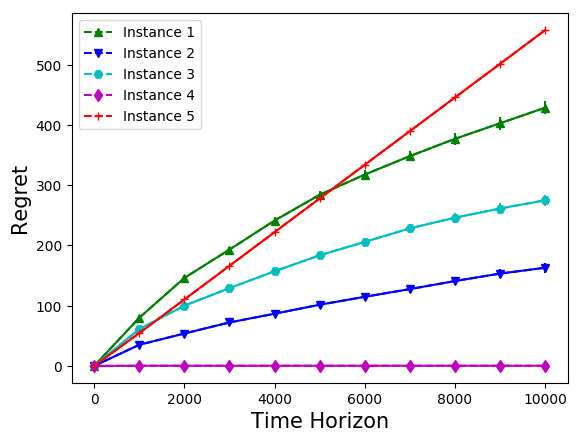
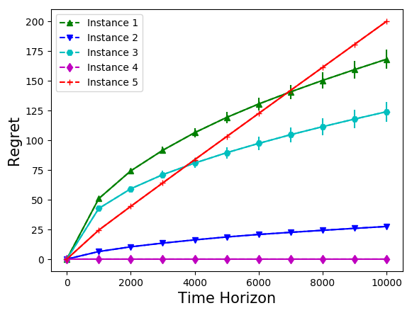
[BSC Dataset] [PIMA Indians Diabetes] [Heart Disease]

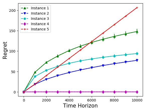
Figure 1: Regret of USS-TS for different problem instances derived from synthetic and real datasets.

Expected Cumulative Regret v/s Time Horizon:

The Regret of USS-TS versus Time Horizon plots for the different problem instances derived from BSC Dataset and two real datasets are shown in Figure 1. These plots verify that any instance that satisfies $\mathrm{WD}$ property has sub-linear regret. Note that USS-TS has linear regret for the Instance $5$ as it does not satisfy $\mathrm{WD}$ property. We also compare the performance of USS-TS with existing UCB based algorithm USS-UCB algorithm of Verma et al. (2019b) with value of $\alpha=0.5$ (best possible parameter value mentioned in the paper) and Algorithm 2 of Hanawal et al. (2017) with value of $\alpha=1.5$ (as used in the paper) on Heart Disease and PIMA Indians Diabetes datasets. As expected, USS-TS outperforms other algorithms with large margins as shown in Fig. 2 (PIMA Indians Diabetes dataset) and Fig. 2 (Heart Disease dataset).

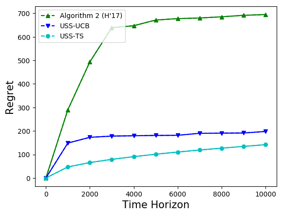
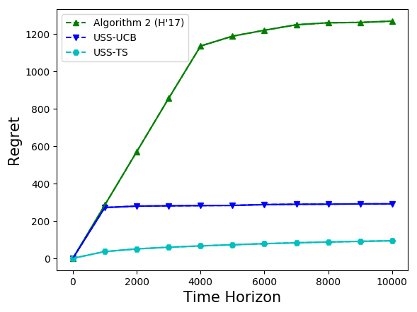
[PIMA Indians Diabetes] [Heart Disease] [BSC Dataset]

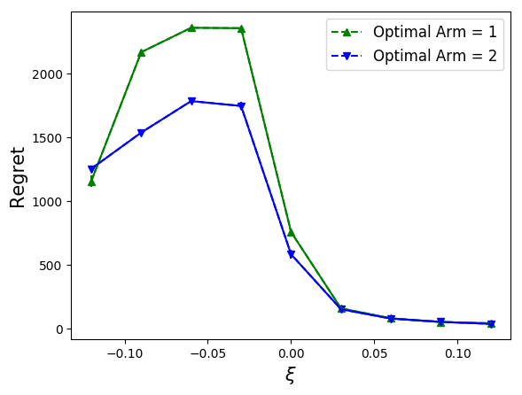
Figure 2: Comparing regret of USS-TS with USS-UCB (Verma et al., 2019b) and Algorithm 2 (Hanawal et al., 2017) for real datasets (Fig. 2 and Fig. 2). Regret behavior of USS-TS versus WD property for BSC Dataset is shown in Fig. 2.

Learnability v/s $\mathrm{WD}$ Property:

We experiment with different problem instances of the BSC dataset to know the relationship between regret of USS-TS and $\mathrm{WD}$ property. We fixed an optimal arm and vary the cumulative cost of using arms in such a way that we pass from the case where $\mathrm{WD}$ property does not hold ($\xi\leq 0$ or $C_{j}-C_{i^{\star}}\in(\gamma_{i^{\star}}-\gamma_{j},p_{i^{\star}j}]$ for any $j>i^{\star}$ where $\xi:=\min_{j>i^{\star}}\xi_{j}$) to the situation where $\mathrm{WD}$ property holds $(\xi>0$). When $\mathrm{WD}$ property does not hold for any problem instance, USS-TS treats a sub-optimal arm as the optimal arm. In such problem instances, as $C_{j}-C_{i^{\star}}$ increases, the regret will also increase due to selection of sub-optimal arm by USS-TS until $\mathrm{WD}$ property does not satisfy for that problem instance. When $\mathrm{WD}$ property does not satisfy for a problem instance then $C_{j}-C_{i^{\star}}\in(\gamma_{i^{\star}}-\gamma_{j},p_{i^{\star}j}]$ holds in such cases, hence, it is easy to verify that $\xi$ can not be smaller than $-\max(p_{i^{\star}j}-(\gamma_{i^{\star}}-\gamma_{j}))$.

We consider the problem instances with the minimum possible value of $\xi$ for which problem instance satisfies $\mathrm{WD}$ property. Then we increase the value of $\xi$ by increasing the cumulative cost of the arm. The regret versus $\xi$ plots for BSC Dataset is shown in Fig. 2. It can be observed that there is a transition at $\xi=0$. Through our experiments, we show that the stronger the $\mathrm{WD}$ property (large value of $\xi$) for the problem instance, it is easier to identify the optimal arm and, hence the less regret is incurred by USS-TS.

6 Conclusion

We studied the unsupervised sequential selection (USS) problem, where both accuracy and cost of using arms are important. It is a variant of the stochastic partial monitoring problem, where the losses are not observed. Still, one can compare the feedback of two arms to see if they agree or disagree. We estimate the disagreement probability between each pair of the arms and develop an algorithm named USS-TS that achieves near-optimal regret. We demonstrate our algorithms’ performance on two real datasets and empirically show that any problem instance satisfying WD property has sub-linear regret. We ignored the inherent side observations due to the arms’ cascade structure. By using these side observations, one can tighten the regret bounds. Another interesting future direction is to develop algorithms that relax the cascade structure assumption and selects the best subset of arms.

Supplementary Material for

‘Thompson Sampling for Unsupervised Sequential Selection’

Appendix A Useful results needed to prove regret bounds of USS-TS

We use the following results in our proofs.

Fact 2 (Chernoff bound for Bernoulli distributed random variables).

Let $X_{1},\ldots,X_{n}$ be i.i.d. Bernoulli distributed random variables. Let $\hat{\mu}_{n}=\frac{1}{n}\sum_{i=1}^{n}X_{i}$ and $\mu=\mathbb{E}\left[X_{i}\right]$. Then, for any $\varepsilon\in(0,1-\mu)$,

$$\mathbb{P}\left\{\hat{\mu}_{n}\geq\mu+\varepsilon\right\}\leq\exp\left(-d(\mu+\varepsilon,\mu)n\right),$$

and, for any $\varepsilon\in(0,\mu)$,

$$\mathbb{P}\left\{\hat{\mu}_{n}\leq\mu-\varepsilon\right\}\leq\exp\left(-d(\mu-\varepsilon,\mu)n\right),$$

where $d(x,\mu)=x\log\left(\frac{x}{\mu}\right)+(1-x)\log\left(\frac{1-x}{1-\mu}\right)$.

See Section 10.1 of Chapter 10 of book ‘Bandit Algorithms’ (Lattimore and Szepesvári, 2020) for proof.

Fact 3 (Pinsker’s Inequality for Bernoulli distributed random variables).

For $p,q\in(0,1)$, the KL divergence between two Bernoulli distributions is bounded as:

$$d(p,q)\geq 2(p-q)^{2}.$$

Fact 4.

Let $x>0$ and $D>0$. Then, for any $a\in(0,1)$,

$$\frac{1}{\exp^{Dx}-1}\leq\begin{cases}\frac{\exp^{-Dx}}{1-a}&\left(x\geq\ln\left(1/a\right)/D\right)\\ \frac{1}{Dx}&\left(x<\ln\left(1/a\right)/D\right).\end{cases}$$

Further, we have,

$$\sum_{x=1}^{n}\frac{1}{\exp^{Dx}-1}\leq\Theta\left(\frac{1}{D^{2}}+\frac{1}{D}\right).$$

Proof.

Using $\exp^{y}\geq y+1$ (by Taylor Series expansion), we have $\frac{1}{\exp^{Dx}-1}\leq\frac{1}{Dx}$ as $\exp^{Dx}-1\geq Dx$. We can re-write, $\frac{1}{\exp^{Dx}-1}=\frac{\exp^{-Dx}}{1-\exp^{-Dx}}$. Since $\exp^{-Dx}$ is strictly decreasing function for all $Dx>0$, it is easy to check that $\exp^{-Dx}\leq a$ holds for any $x\geq\ln\left(1/a\right)/D$ and $a\in(0,1)$. Hence, $\frac{\exp^{-Dx}}{1-\exp^{-Dx}}\leq\frac{\exp^{-Dx}}{1-a}$ for all $x\geq\ln\left(1/a\right)/D$.

Now we will prove the second part,

$$\sum_{x=1}^{n}\frac{1}{\exp^{Dx}-1} \leq\frac{\ln(1/a)}{D^{2}}+\sum_{x\geq\ln\left(1/a\right)/D}^{n}\frac{\exp^{-Dx}}{1-a}$$

$$\leq\frac{\ln(1/a)}{D^{2}}+\frac{1}{(1-a)}\int_{x=0}^{\infty}\exp^{-Dx}dx$$

$$=\frac{\ln(1/a)}{D^{2}}+\frac{1}{(1-a)}\left.\left(\frac{\exp^{-Dx}}{-D}\right)\right|_{x=0}^{\infty}$$

$$=\frac{\ln(1/a)}{D^{2}}+\frac{1}{(1-a)}\left(0-\frac{\exp^{0}}{-D}\right)$$

$$=\frac{\ln(1/a)}{D^{2}}+\frac{1}{(1-a)D}$$

$$\implies\sum_{x=1}^{n}\frac{1}{\exp^{Dx}-1} \leq\Theta\left(\frac{1}{D^{2}}+\frac{1}{D}\right).\qed$$

Fact 5.

Let $\varepsilon\in(0,1)$ and $0<x<y<z<1$. If $d(y,z)=d(x,z)/(1+\varepsilon)$ then

$$y-x\geq\frac{\varepsilon}{1+\varepsilon}\cdot\frac{d(x,z)}{\ln\left(\frac{z(1-x)}{x(1-z)}\right)}.$$

Proof.

By definition

$$d(p,q) =p\ln\frac{p}{q}+(1-p)\ln\left(\frac{1-p}{1-q}\right)$$

$$=\ln\left(\left(\frac{p}{q}\right)^{p}\left(\frac{1-p}{1-q}\right)^{1-p}\right)$$

$$=\ln\left(\left(\frac{q(1-p)}{p(1-q)}\right)^{-p}\right)+\ln\left(\frac{1-p}{1-q}\right)$$

$$\implies d(p,q) =-p\ln\left(\frac{q(1-p)}{p(1-q)}\right)+\ln\left(\frac{1-p}{1-q}\right).$$

Set $l(p,q)=\ln\left(\frac{q(1-p)}{p(1-q)}\right)$. Note that $l(p,\cdot)$ is a strictly decreasing function of $p$ and positive for all $p<q$. We can re-arrange above equation as

$$p\cdot l(p,q)=-d(p,q)+\ln\left(\frac{1-p}{1-q}\right).$$

Using above equation, we have

$$y\cdot l(y,z)-x\cdot l(x,z) =-d(y,z)+\ln\left(\frac{1-y}{1-z}\right)+d(x,z)-\ln\left(\frac{1-x}{1-z}\right).$$

Using $$d(y,z)=d(x,z)/(1+\varepsilon)$$,

$$y\cdot l(y,z)-x\cdot l(x,z) =\frac{\varepsilon}{1+\varepsilon}d(x,z)+\ln\left(\frac{1-y}{1-x}\right).$$

After adding $$y(l(x,z)-l(y,z))$$ both side, we have

$$(y-x)l(x,z) =\frac{\varepsilon}{1+\varepsilon}d(x,z)+\ln\left(\frac{1-y}{1-x}\right)+y(l(x,z)-l(y,z)).$$

Using $$l(x,z)=\ln\left(\frac{z(1-x)}{x(1-z)}\right) l(y,z)=\ln\left(\frac{z(1-y)}{y(1-z)}\right)$$ and

$$=\frac{\varepsilon}{1+\varepsilon}d(x,z)+\ln\left(\frac{1-y}{1-x}\right)+y\ln\left(\frac{y(1-x)}{x(1-y)}\right)$$

$$=\frac{\varepsilon}{1+\varepsilon}d(x,z)+\ln\left(\left(\frac{y(1-x)}{x(1-y)}\right)^{y}\cdot\frac{1-y}{1-x}\right)$$

$$=\frac{\varepsilon}{1+\varepsilon}d(x,z)+\ln\left(\left(\frac{y}{x}\right)^{y}\left(\frac{1-y}{1-x}\right)^{1-y}\right)$$

$$=\frac{\varepsilon}{1+\varepsilon}d(x,z)+d(y,x)$$

As $$d(p,q)\geq 0 l(x,z)$$ and dividing both side by ,

$$\implies y-x \geq\frac{\varepsilon}{1+\varepsilon}\cdot\frac{d(x,z)}{l(x,z)}.$$

Substituting value of $l(x,z)$ in the above equation, we get

$$y-x\geq\frac{\varepsilon}{1+\varepsilon}\cdot\frac{d(x,z)}{\ln\left(\frac{z(1-x)}{x(1-z)}\right)}.\qed$$

Appendix B Leftover proofs from Section 4

See 4

Proof.

Applying 3 and properties of conditional expectations, we have

$$\sum_{t=1}^{T}\mathbb{P}\left\{I_{t}=j,j<{i^{\star}}\right\} =\sum_{t=1}^{T}\mathbb{E}\left[\mathbb{P}\left\{I_{t}=j,j<{i^{\star}}|\mathcal{H}_{t}\right\}\right].$$

As $$q_{j,t} \mathcal{H}_{t}$$ is fixed given ,

$$\implies\sum_{t=1}^{T}\mathbb{P}\left\{I_{t}=j,j<{i^{\star}}\right\} \leq\sum_{t=1}^{T}\mathbb{E}\left[\frac{(1-q_{j,t})}{q_{j,t}}\mathbb{P}\left\{I_{t}\geq i^{\star}|\mathcal{H}_{t}\right\}\right]$$

$$\leq\sum_{t=1}^{T}\mathbb{E}\left[\mathbb{E}\left[\frac{(1-q_{j,t})}{q_{j,t}}\mathds{1}_{\left\{I_{t}\geq i^{\star}\right\}}|\mathcal{H}_{t}\right]\right].$$

Using law of iterated expectations,

$$\implies\sum_{t=1}^{T}\mathbb{P}\left\{I_{t}=j,j<{i^{\star}}\right\} \leq\sum_{t=1}^{T}\mathbb{E}\left[\frac{(1-q_{j,t})}{q_{j,t}}\mathds{1}_{\left\{I_{t}\geq i^{\star}\right\}}\right].$$ (14)

Let $s_{m}$ denote the time step at which the output of arm $i^{\star}$ is observed for the $m^{th}$ time for $m\geq 1$, and let $s_{0}=0$. For $j<i^{\star}$, whenever the output from arm $i^{\star}$ is observed then the output from arm $j$ is also observed due to the cascade structure. Note that $q_{j,t}=\mathbb{P}\left\{\tilde{p}_{i^{\star}j}^{(t)}>p_{i^{\star}j}-\xi_{j}|\mathcal{H}_{t}\right\}$ changes only when the distribution of $\tilde{p}_{i^{\star}j}^{(t)}$ changes, that is, only on the time step when the feedback from arms $i^{\star}$ and $j$ are observed. It only happens when selected arm $I_{t}\geq{i^{\star}}$. Hence, $q_{j,t}$ is the same at all time steps $t\in\{s_{m}+1,\ldots,s_{m+1}\}$ for every $m$. Using this fact, we can decompose the right hand side term in Eq. 14 as follows,

$$\sum_{t=1}^{T}\mathbb{E}\left[\frac{(1-q_{j,t})}{q_{j,t}}\mathds{1}_{\left\{I_{t}\geq i^{\star}\right\}}\right] =\sum_{m=0}^{T-1}\mathbb{E}\left[\frac{(1-q_{j,s_{m}+1})}{q_{j,s_{m}+1}}\sum_{t=s_{m}+1}^{s_{m+1}}\mathds{1}_{\left\{I_{t}\geq i^{\star}\right\}}\right]$$

$$\leq\sum_{m=0}^{T-1}\mathbb{E}\left[\frac{(1-q_{j,s_{m}+1})}{q_{j,s_{m}+1}}\right]$$

$$=\sum_{k=0}^{T-1}\mathbb{E}\left[\frac{1}{q_{j,s_{m}+1}}-1\right].$$

Using above bound in Eq. 14, we get

$$\sum_{t=1}^{T}\mathbb{P}\left\{I_{t}=j,j<{i^{\star}}\right\}\leq\sum_{m=0}^{T-1}\mathbb{E}\left[\frac{1}{q_{j,s_{m}+1}}-1\right].$$

Substituting the bound from 2 with $\mu=p_{i^{\star}j},x=p_{i^{\star}j}-\xi_{j},\Delta(x)=\xi_{j},$ and $q_{n}(x)=q_{j,s_{m}}$, we obtain the following bound,

$$\sum_{t=1}^{T}\mathbb{P}\left\{I_{t}=j,j<{i^{\star}}\right\}\leq\frac{24}{\xi_{j}^{2}}+\sum_{s\geq 8/\xi_{j}}\Theta\left(\exp^{-{s\xi_{j}^{2}}/{2}}+\frac{\exp^{-{sd(p_{i^{\star}j}-\xi_{j},p_{i^{\star}j})}}}{(s+1)\xi_{j}^{2}}+\frac{1}{\exp^{{s\xi_{j}^{2}}/{4}}-1}\right).\qed$$

See 6

Proof.

Let $s_{m}$ denote the time step at which the outputs of arm $i^{\star}$ and $j$ is observed for the $m^{th}$ time for $m\geq 1$, and let $s_{0}=0$. Note that probability $\mathbb{P}\left\{\hat{p}_{i^{\star}j}^{(t)}>x_{j}\right\}$ changes when the outputs from both arm $i^{\star}$ and $j$ are observed. Hence, we have

$$\sum_{t=1}^{T}\mathbb{P}\left\{\hat{p}_{i^{\star}j}^{(t)}>x_{j}\right\} \leq\sum_{m=0}^{T-1}\mathbb{P}\left\{\hat{p}_{i^{\star}j}(s_{m+1})>x_{j}\right\}$$

$$=\sum_{m=0}^{T-1}\mathbb{P}\left\{\hat{p}_{i^{\star}j}(s_{m+1})-p_{i^{\star}j}>x_{j}-p_{i^{\star}j}\right\}$$

$$\leq\sum_{m=0}^{T-1}\exp^{-kd(p_{i^{\star}j}+x_{j}-p_{i^{\star}j},p_{i^{\star}j})}\hskip 28.45274pt\text{(using \lx@cref{creftype~refnum}{fact:chernoff}})$$

$$=\sum_{m=0}^{T-1}\exp^{-kd(x_{j},p_{i^{\star}j})}.$$

Using $\sum_{s\geq 0}\exp^{-sa}\leq 1/a$, we get

$$\sum_{t=1}^{T}\mathbb{P}\left\{\hat{p}_{i^{\star}j}^{(t)}>x_{j}\right\}\leq\frac{1}{d(x_{j},p_{i^{\star}j})}.\qed$$

See 7

Proof.

Let $p_{i^{\star}j}<x_{j}<y_{j}<p_{i^{\star}j}+\xi_{j}$ for any $j>i^{\star}$. Than,

$$\sum_{t=1}^{T}\mathbb{P}\left\{j\succ_{t}i^{\star},j>{i^{\star}}\right\} =\sum_{t=1}^{T}\mathbb{P}\left\{\tilde{p}_{i^{\star}j}^{(t)}>p_{i^{\star}j}+\xi_{j}\right\}$$

$$\leq\sum_{t=1}^{T}\mathbb{P}\left\{\tilde{p}_{i^{\star}j}^{(t)}>y_{j}\right\}$$

$$\leq\sum_{t=1}^{T}\mathbb{P}\left\{\hat{p}_{i^{\star}j}^{(t)}\leq x_{j},\tilde{p}_{i^{\star}j}^{(t)}>y_{j}\right\}+\sum_{t=1}^{T}\mathbb{P}\left\{\hat{p}_{i^{\star}j}^{(t)}>x_{j}\right\}.$$

Using 6 and 5, we have

$$\sum_{t=1}^{T}\mathbb{P}\left\{j\succ_{t}i^{\star},j>{i^{\star}}\right\}\leq\frac{\ln T}{d(x_{j},y_{j})}+1+\frac{1}{d(x_{j},p_{i^{\star}j})}.$$

For $\varepsilon\in(0,1)$, we set $x_{j}\in(p_{i^{\star}j},p_{i^{\star}j}+\xi_{j})$ such that $d(x_{j},p_{i^{\star}j}+\xi_{j})=d(p_{i^{\star}j},p_{i^{\star}j}+\xi_{j})/(1+\varepsilon)$, and set $y_{j}\in(x_{j},p_{i^{\star}j}+\xi_{j})$ such that $d(x_{j},y_{j})=d(x_{j},p_{i^{\star}j}+\xi_{j})/(1+\varepsilon)=d(p_{i^{\star}j},p_{i^{\star}j}+\xi_{j})/(1+\varepsilon)^{2}$. Then this gives

$$\frac{\ln(T)}{d(x_{j},y_{j})}=(1+\varepsilon)^{2}\frac{\ln(T)}{d(p_{i^{\star}j},p_{i^{\star}j}+\xi_{j})}.$$

Using 5, if $\varepsilon\in(0,1)$, $x_{j}\in(p_{i^{\star}j},p_{i^{\star}j}+\xi_{j})$, and $d(x_{j},p_{i^{\star}j}+\xi_{j})=d(p_{i^{\star}j},p_{i^{\star}j}+\xi_{j})/(1+\varepsilon)$ then

$$x_{j}-p_{i^{\star}j}\geq\frac{\varepsilon}{1+\varepsilon}.\frac{d(p_{i^{\star}j},p_{i^{\star}j}+\xi_{j})}{\ln\left(\frac{(p_{i^{\star}j}+\xi_{j})(1-p_{i^{\star}j})}{p_{i^{\star}j}(1-p_{i^{\star}j}-\xi_{j})}\right)}.$$

Using Pinsker’s Inequality (3), $1/d(x_{j},p_{i^{\star}j})\leq 1/2(x_{j}-p_{i^{\star}j})^{2}=O({1}/{\varepsilon^{2}})$ where big-Oh is hiding functions of the $p_{i^{\star}j}$ and $\xi_{j}$,

$$\sum_{t=1}^{T}\mathbb{P}\left\{j\succ_{t}{i^{\star}},j>i^{\star}\right\} \leq(1+\varepsilon)^{2}\frac{\ln(T)}{d(p_{i^{\star}j},p_{i^{\star}j}+\xi_{j})}+O\left(\frac{1}{\varepsilon^{2}}\right)$$

$$\leq(1+3\varepsilon)\frac{\ln(T)}{d(p_{i^{\star}j},p_{i^{\star}j}+\xi_{j})}+O\left(\frac{1}{\varepsilon^{2}}\right)$$

$$\leq(1+\varepsilon^{\prime})\frac{\ln(T)}{d(p_{i^{\star}j},p_{i^{\star}j}+\xi_{j})}+O\left(\frac{1}{{\varepsilon^{\prime}}^{2}}\right),$$

where $\varepsilon^{\prime}=3\varepsilon$ and the big-Oh above hides $p_{i^{\star}j}$ and $\xi_{j}$ in addition to the absolute constants. Replacing $\varepsilon$ by $\varepsilon^{\prime}$ completes the proof. ∎

See 1

Proof.

Let $M_{j}(T)$ is the number of times arm $j$ is selected by USS-TS. Than, the regret is

$${\mathfrak{R}_{T}} =\sum_{j\in[K]}\mathbb{E}\left[M_{j}(T)\right]\Delta_{j}=\sum_{j\in[K]}\mathbb{E}\left[\sum_{t=1}^{T}\mathds{1}_{\left\{I_{t}=j\right\}}\right]\Delta_{j}$$

$$=\sum_{j\in[K]}\sum_{t=1}^{T}\mathbb{E}\left[\mathds{1}_{\left\{I_{t}=j\right\}}\right]\Delta_{j}=\sum_{j\in[K]}\sum_{t=1}^{T}\mathbb{P}\left\{I_{t}=j\right\}\Delta_{j}$$

$$=\sum_{j\in[K]}\sum_{t=1}^{T}\mathbb{P}\left\{I_{t}=j,j\neq{i^{\star}}\right\}\Delta_{j}$$

$$\implies{\mathfrak{R}_{T}} =\sum_{j<i^{\star}}\sum_{t=1}^{T}\mathbb{P}\left\{I_{t}=j,j<i^{\star}\right\}\Delta_{j}+\sum_{j>i^{\star}}\sum_{t=1}^{T}\mathbb{P}\left\{I_{t}=j,j>i^{\star}\right\}\Delta_{j}$$ (15)

First, we bound the first of term of summation. From 4, we have

$$\sum_{t=1}^{T}\mathbb{P}\left\{I_{t}=j,j<i^{\star}\right\}\leq\frac{24}{\xi_{j}^{2}}+\sum_{s\geq 8/\xi_{j}}\Theta\left(\exp^{-{s\xi_{j}^{2}}/{2}}+\frac{\exp^{-{sd(p_{i^{\star}j}-\xi_{j},p_{i^{\star}j})}}}{(s+1)\xi_{j}^{2}}+\frac{1}{\exp^{{s\xi_{j}^{2}}/{4}}-1}\right).$$

Using $\sum_{s\geq 0}\exp^{-sa}\leq 1/a$, $d(p_{i^{\star}j}-\xi_{j},p_{i^{\star}j})\leq 2\xi_{j}^{2}$ (3), and 4, we have

$$\sum_{t=1}^{T}\mathbb{P}\left\{I_{t}=j,j<i^{\star}\right\} \leq\frac{24}{\xi_{j}^{2}}+\Theta\left(\frac{1}{\xi_{j}^{2}}+\frac{1}{\xi_{j}^{4}}+\left(\frac{1}{\xi_{j}^{4}}+\frac{1}{\xi_{j}^{2}}\right)\right)\leq O(1).$$ (16)

If arm $I_{t}>{i^{\star}}$ is selected then there exists at least one arm $k_{1}>{i^{\star}}$ which must be preferred over ${i^{\star}}$. If the index of arm $k_{1}$ is smaller than the selected arm, then there must be an arm $k_{2}>k_{1}$, which must be preferred over $k_{1}$. By transitivity property, arm $k_{2}$ is also preferred over ${i^{\star}}$. If the index of arm $k_{2}$ is still smaller of the selected arm, we can repeat the same argument. Eventually, we can find an arm $k^{\prime}$ whose index is larger than the selected arm, and it is preferred over arm $k_{i},\ldots,k_{1},{i^{\star}}$. Note that the selected arm must be preferred over $k^{\prime}$; hence the selected arm is also preferred over ${i^{\star}}$. We can write it as follows:

$$\sum_{t=1}^{T}\mathbb{P}\left\{I_{t}=j,j>i^{\star}\right\}\Delta_{j}= ~{}\sum_{t=1}^{T}\mathbb{P}\left\{I_{t}=j,j>i^{\star},k^{\prime}\succ_{t}k,k\succ_{t}{i^{\star}},k^{\prime}>j,k>{i^{\star}}\right\}\Delta_{j}$$

$$= ~{}\sum_{t=1}^{T}\mathbb{P}\left\{I_{t}=j,j>i^{\star},k^{\prime}\succ_{t}{i^{\star}},k^{\prime}>j\right\}\Delta_{j}\mbox{\hskip 5.69054pt (\lx@cref{creftype~refnum}{def:trans_prop})}$$

$$= ~{}\sum_{t=1}^{T}\mathbb{P}\left\{j\succ_{t}k,\forall k>j,j>i^{\star},k^{\prime}\succ_{t}{i^{\star}},k^{\prime}>j\right\}\Delta_{j}\mbox{\hskip 2.84526pt(\lx@cref{creftype~refnum}{lem:Bx})}$$

$$= ~{}\sum_{t=1}^{T}\mathbb{P}\left\{j\succ_{t}k,\forall k>j,j>i^{\star},j\succ_{t}{i^{\star}}\right\}\Delta_{j}\mbox{\hskip 5.69054pt (\lx@cref{creftype~refnum}{def:trans_prop})}$$

$$\implies\sum_{t=1}^{T}\mathbb{P}\left\{I_{t}=j,j>i^{\star}\right\}\Delta_{j}\leq ~{}\sum_{t=1}^{T}\mathbb{P}\left\{j\succ_{t}{i^{\star}},j>{i^{\star}}\right\}\Delta_{j}.$$ (17)

Using 7 to upper bound $\sum_{t=1}^{T}$ $\mathbb{P}\left\{j\succ_{t}{i^{\star}},j>i^{\star}\right\}\Delta_{j}$ and with Eq. 16, we get

$${\mathfrak{R}_{T}} \leq O(1)+\sum_{j>i^{\star}}\left((1+\varepsilon)\frac{\ln(T)}{d(p_{i^{\star}j},p_{i^{\star}j}+\xi_{j})}+O\left(\frac{1}{\varepsilon^{2}}\right)\right)\Delta_{j}$$

$$\implies{\mathfrak{R}_{T}} \leq\sum_{j>i^{\star}}\ \frac{(1+\varepsilon)\ln(T)}{d(p_{i^{\star}j},p_{i^{\star}j}+\xi_{j})}\Delta_{j}+O\left(\frac{K-i^{\star}}{\varepsilon^{2}}\right).\qed$$

See 2

Proof.

Let $M_{j}(T)$ is the number of times arm $j$ preferred over the optimal arm in $T$ rounds. From 4, for any $j<i^{\star}$, we have

$$\mathbb{E}\left[M_{j}(T)\right] =\sum_{t=1}^{T}\mathbb{P}\left\{I_{t}=j,j<i^{\star}\right\}$$

$$\leq\frac{24}{\xi_{j}^{2}}+\sum_{s\geq 8/\xi_{j}}\Theta\left(\exp^{-{s\xi_{j}^{2}}/{2}}+\frac{\exp^{-{sd(p_{i^{\star}j}-\xi_{j},p_{i^{\star}j})}}}{(s+1)\xi_{j}^{2}}+\frac{1}{\exp^{{s\xi_{j}^{2}}/{4}}-1}\right).$$

It is east to show that $\frac{\exp^{-{sd(p_{i^{\star}j}-\xi_{j},p_{i^{\star}j})}}}{(s+1)\xi_{j}^{2}}\leq\frac{1}{(s+1)\xi_{j}^{2}}$ and ${\exp^{{s\xi_{j}^{2}}/{4}}-1}\geq{s\xi_{j}^{2}}/4$ (as $\exp^{y}\geq y+1$),

$$\mathbb{E}\left[M_{j}(T)\right]\leq\frac{24}{\xi_{j}^{2}}+\sum_{s\geq 8/\xi_{j}}\Theta\left(\frac{1}{\xi_{j}^{2}}+\frac{1}{(s+1)\xi_{j}^{2}}+\frac{4}{s\xi_{j}^{2}}\right).$$

By using $\sum_{s\geq 0}\exp^{-sa}\leq 1/a$ and $\sum_{s=1}^{T}(1/s)=\log T$,

$$\mathbb{E}\left[M_{j}(T)\right] \leq\frac{24}{\xi_{j}^{2}}+\Theta\left(\frac{1}{\xi_{j}^{2}}+\frac{\ln T}{\xi_{j}^{2}}\right)\implies\mathbb{E}\left[M_{j}(T)\right]\leq O\left(\frac{\ln T}{\xi_{j}^{2}}\right).$$ (18)

For any $j>i^{\star}$, using 5 and 6 with Eq. 17, we have

$$\mathbb{E}\left[M_{j}(T)\right]=\sum_{t=1}^{T}\mathbb{P}\left\{I_{t}=j,j>i^{\star}\right\}\leq\sum_{t=1}^{T}\mathbb{P}\left\{j\succ_{t}{i^{\star}},j>i^{\star}\right\}\leq\frac{\ln T}{d(x_{j},y_{j})}+1+\frac{1}{d(x_{j},p_{i^{\star}j})}.$$

By setting $x_{j}=p_{i^{\star}j}+\frac{\xi_{j}}{3}$ and $y_{j}=p_{i^{\star}j}+\frac{2\xi_{j}}{3}$, we have $d(x_{j},y_{j})\geq\frac{2\xi_{j}^{2}}{9}$ and $d(x_{j},p_{i^{\star}j})\geq\frac{2\xi_{j}^{2}}{9}$ (using 3).

$$\mathbb{E}\left[M_{j}(T)\right] \leq\frac{9\ln T}{2\xi_{j}^{2}}+1+\frac{9}{2\xi_{j}^{2}}$$

$$\implies\mathbb{E}\left[M_{j}(T)\right] \leq O\left(\frac{\ln T}{\xi_{j}^{2}}\right).$$ (19)

The regret of USS-TS is given by

$${\mathfrak{R}_{T}}=\sum\limits_{j\neq i^{\star}}\mathbb{E}\left[M_{j}(T)\right]\Delta_{j}=\sum\limits_{j<i^{\star}}\mathbb{E}\left[M_{j}(T)\right]\Delta_{j}+\sum\limits_{j>i^{\star}}\mathbb{E}\left[M_{j}(T)\right]\Delta_{j}$$

Recall $\Delta_{j}=C_{j}+\gamma_{j}-(C_{i^{\star}}+\gamma_{i^{\star}})$ and for any two arms $i$ and $j$, $0\leq p_{ij}-(\gamma_{j}-\gamma_{i^{\star}})\leq\beta$. By using Eq. (8a) for $j<i^{\star}$, we have $\Delta_{j}=\xi_{j}-(p_{i^{\star}j}-(\gamma_{i^{\star}}-\gamma_{j}))\implies\Delta_{j}\leq\xi_{j}$, and using Eq. (8b) for $j>i^{\star}$, we have $\Delta_{j}=\xi_{j}+(p_{i^{\star}j}-(\gamma_{i^{\star}}-\gamma_{j}))\implies\Delta_{j}\leq\xi_{j}+\beta$. Replacing $\Delta_{j}$,

$$\Rightarrow{\mathfrak{R}_{T}}\leq\sum\limits_{j<i^{\star}}\mathbb{E}\left[M_{j}(T)\right]\xi_{j}+\sum\limits_{j>i^{\star}}\mathbb{E}\left[M_{j}(T)\right](\xi_{j}+\beta).$$

Let $0<\xi^{\prime}<1$. Then ${\mathfrak{R}_{T}}$ can be written as:

$${\mathfrak{R}_{T}} \leq\sum\limits_{\begin{subarray}{c}\xi^{\prime}>\xi_{j}\\ j<i^{\star}\end{subarray}}\mathbb{E}\left[M_{j}(T)\right]\xi_{j}+\sum\limits_{\begin{subarray}{c}\xi^{\prime}<\xi_{j}\\ j<i^{\star}\end{subarray}}\mathbb{E}\left[M_{j}(T)\right]\xi_{j}$$

$$\qquad+\sum\limits_{\begin{subarray}{c}\xi^{\prime}>\xi_{j}\\ j>i^{\star}\end{subarray}}\mathbb{E}\left[M_{j}(T)\right](\xi_{j}+\beta)+\sum\limits_{\begin{subarray}{c}\xi^{\prime}<\xi_{j}\\ j>i^{\star}\end{subarray}}\mathbb{E}\left[M_{j}(T)\right](\xi_{j}+\beta).$$

Using $\sum\limits_{\xi^{\prime}>\xi_{j}}\mathbb{E}\left[M_{j}(T)\right]\leq T$ for any $j$ such that $\xi^{\prime}>\xi_{j}$,

$${\mathfrak{R}_{T}} \leq T\xi^{\prime}+\sum\limits_{\begin{subarray}{c}\xi^{\prime}<\xi_{j}\\ j<i^{\star}\end{subarray}}\mathbb{E}\left[M_{j}(T)\right]\xi_{j}+\sum\limits_{\begin{subarray}{c}\xi^{\prime}<\xi_{j}\\ j>i^{\star}\end{subarray}}\mathbb{E}\left[M_{j}(T)\right](\xi_{j}+\beta).$$

Substituting the value of ${\mathfrak{R}_{T}}$ from Eq. 18 and Eq. 19,

$${\mathfrak{R}_{T}} \leq T\xi^{\prime}+\sum\limits_{\begin{subarray}{c}\xi^{\prime}<\xi_{j}\\ j<i^{\star}\end{subarray}}O\left(\frac{\xi_{j}\ln T}{\xi_{j}^{2}}\right)+\sum\limits_{\begin{subarray}{c}\xi^{\prime}<\xi_{j}\\ j>i^{\star}\end{subarray}}O\left(\frac{(\xi_{j}+\beta)\ln T}{\xi_{j}^{2}}\right)$$

$$\leq T\xi^{\prime}+\sum\limits_{\begin{subarray}{c}\xi^{\prime}<\xi_{j}\\ j<i^{\star}\end{subarray}}O\left(\frac{\ln T}{\xi_{j}}\right)+\sum\limits_{\begin{subarray}{c}\xi^{\prime}<\xi_{j}\\ j>i^{\star}\end{subarray}}O\left(\frac{\ln T}{\xi_{j}}+\frac{\beta\ln T}{\xi_{j}^{2}}\right)$$

$$\leq T\xi^{\prime}+O\left(\frac{K\ln T}{\xi^{\prime}}\right)+O\left(\frac{K\ln T}{\xi^{\prime}}+\frac{\beta K\ln T}{{\xi^{\prime}}^{2}}\right)$$

$$=T\xi^{\prime}+O\left(K\ln T\left(\frac{1}{\xi^{\prime}}+\frac{\beta}{{\xi^{\prime}}^{2}}\right)\right)$$

Let there exist a variable $$\alpha O\left(K\ln T\left(\frac{1}{\xi^{\prime}}+\frac{\beta}{{\xi^{\prime}}^{2}}\right)\right)\leq\alpha K\ln T\left(\frac{1}{\xi^{\prime}}+\frac{\beta}{{\xi^{\prime}}^{2}}\right)$$ such that ,

$$\implies{\mathfrak{R}_{T}} \leq=T\xi^{\prime}+\alpha K\ln T\left(\frac{1}{\xi^{\prime}}+\frac{\beta}{{\xi^{\prime}}^{2}}\right).$$ (20)

Consider $\mathcal{P}_{\mathrm{WD}}$ class of problems. As $\xi^{\prime}<1$ and $\beta\leq 2$ (as arms in the cascade may not be ordered by their error-rates, it is possible that $\gamma_{i}<\gamma_{j}$), we have $\left(\frac{1}{\xi^{\prime}}+\frac{\beta}{{\xi^{\prime}}^{2}}\right)\leq\frac{\beta+1}{{\xi^{\prime}}^{2}}\leq\frac{3}{{\xi^{\prime}}^{2}}$,

$${\mathfrak{R}_{T}} \leq=T\xi^{\prime}+\frac{3\alpha K\ln T}{{\xi^{\prime}}^{2}}.$$

Choose $$\xi^{\prime}=\left(\frac{6\alpha K\ln T}{T}\right)^{1/3}$$ which maximize above upper bound and we get,

$${\mathfrak{R}_{T}} \leq\left(6\alpha K\ln T\right)^{1/3}T^{2/3}+\frac{\left(6\alpha K\ln T\right)^{1/3}}{2}T^{2/3}$$

$$\implies{\mathfrak{R}_{T}} \leq 2\left(6\alpha K\ln T\right)^{1/3}T^{2/3}=O\left(\left(K\ln T\right)^{1/3}T^{2/3}\right)$$

It completes our proof for the case when any problem instance belongs to $\mathcal{P}_{\mathrm{WD}}$.

Now we consider any problem instance $\theta\in\mathcal{P}_{\mathrm{SD}}$. For any $\theta\in\mathcal{P}_{\mathrm{SD}}\Rightarrow\forall j\in[K],\;p_{ij}=\gamma_{i}-\gamma_{j}\implies\beta=0$ (Setting $\mathbb{P}\left\{Y^{i}=Y,Y^{j}\neq Y\right\}=0$ for $j>i$ in Proposition 3 of Hanawal et al. (2017)). We can rewrite Eq. 20 as

$${\mathfrak{R}_{T}} \leq T\xi^{\prime}+\frac{\alpha K\ln T}{{\xi^{\prime}}}.$$

Choose $$\xi^{\prime}=\left(\frac{\alpha K\ln T}{T}\right)^{1/2}$$ which maximize above upper bound and we get,

$$\implies{\mathfrak{R}_{T}} \leq 2\left(\alpha KT\ln T\right)^{1/2}=O\left(\sqrt{KT\ln T}\right)$$

This complete proof for second part of Theorem 2. ∎

References

- Agrawal and Goyal (2012) Shipra Agrawal and Navin Goyal. Analysis of thompson sampling for the multi-armed bandit problem. In Conference on Learning Theory, pages 39–1, 2012.
- Agrawal and Goyal (2013) Shipra Agrawal and Navin Goyal. Further optimal regret bounds for thompson sampling. In Artificial intelligence and statistics, pages 99–107, 2013.
- Alon et al. (2013) Noga Alon, Nicolo Cesa-Bianchi, Claudio Gentile, and Yishay Mansour. From bandits to experts: A tale of domination and independence. In Advances in Neural Information Processing Systems, pages 1610–1618, 2013.
- Alon et al. (2015) Noga Alon, Nicolo Cesa-Bianchi, Ofer Dekel, and Tomer Koren. Online learning with feedback graphs: Beyond bandits. In Annual Conference on Learning Theory, volume 40. Microtome Publishing, 2015.
- Auer et al. (2002) Peter Auer, Nicolo Cesa-Bianchi, and Paul Fischer. Finite-time analysis of the multiarmed bandit problem. Machine learning, pages 235–256, 2002.
- Bartók and Szepesvári (2012) Gábor Bartók and Csaba Szepesvári. Partial monitoring with side information. In International Conference on Algorithmic Learning Theory, pages 305–319. Springer, 2012.
- Bartók et al. (2014) Gábor Bartók, Dean P Foster, Dávid Pál, Alexander Rakhlin, and Csaba Szepesvári. Partial monitoring—classification, regret bounds, and algorithms. Mathematics of Operations Research, 39(4):967–997, 2014.
- Bonald and Combes (2017) Thomas Bonald and Richard Combes. A minimax optimal algorithm for crowdsourcing. In Advances in Neural Information Processing Systems, pages 4352–4360, 2017.
- Bubeck et al. (2012) Sébastien Bubeck, Nicolo Cesa-Bianchi, et al. Regret analysis of stochastic and nonstochastic multi-armed bandit problems. Foundations and Trends® in Machine Learning, 5(1):1–122, 2012.
- Cesa-Bianchi et al. (2006) Nicolo Cesa-Bianchi, Gábor Lugosi, and Gilles Stoltz. Regret minimization under partial monitoring. Mathematics of Operations Research, 31(3):562–580, 2006.
- Chapelle and Li (2011) Olivier Chapelle and Lihong Li. An empirical evaluation of thompson sampling. In Advances in neural information processing systems, pages 2249–2257, 2011.
- Chen et al. (2012) Minmin Chen, Zhixiang Xu, Kilian Weinberger, Olivier Chapelle, and Dor Kedem. Classifier cascade for minimizing feature evaluation cost. In Artificial Intelligence and Statistics, pages 218–226, 2012.
- Detrano (1998) Robert Detrano. V.A. Medical Center, Long Beach and Cleveland Clinic Foundation: Robert Detrano, MD, Ph.D., Donor: David W. Aha, 1998. URL https://archive.ics.uci.edu/ml/datasets/Heart+Disease.
- Garivier and Cappé (2011) Aurélien Garivier and Olivier Cappé. The kl-ucb algorithm for bounded stochastic bandits and beyond. In Proceedings of the 24th annual Conference On Learning Theory, pages 359–376, 2011.
- Hanawal et al. (2017) Manjesh Hanawal, Csaba Szepesvari, and Venkatesh Saligrama. Unsupervised sequential sensor acquisition. In Artificial Intelligence and Statistics, pages 803–811, 2017.
- Kaggle (2016) UCI Machine Learning, Kaggle. Pima Indians Diabetes Database, 2016. URL https://www.kaggle.com/uciml/pima-indians-diabetes-database.
- Kaufmann et al. (2012) Emilie Kaufmann, Nathaniel Korda, and Rémi Munos. Thompson sampling: An asymptotically optimal finite-time analysis. In International Conference on Algorithmic Learning Theory, pages 199–213. Springer, 2012.
- Kleindessner and Awasthi (2018) Matthäus Kleindessner and Pranjal Awasthi. Crowdsourcing with arbitrary adversaries. In International Conference on Machine Learning, pages 2713–2722, 2018.
- Lattimore and Szepesvári (2020) Tor Lattimore and Csaba Szepesvári. Bandit algorithms, 2020.
- Mannor and Shamir (2011) Shie Mannor and Ohad Shamir. From bandits to experts: On the value of side-observations. In Advances in Neural Information Processing Systems, pages 684–692, 2011.
- Trapeznikov and Saligrama (2013) Kirill Trapeznikov and Venkatesh Saligrama. Supervised sequential classification under budget constraints. In Artificial Intelligence and Statistics, pages 581–589, 2013.
- Verma et al. (2019a) Arun Verma, Manjesh Hanawal, Arun Rajkumar, and Raman Sankaran. Censored semi-bandits: A framework for resource allocation with censored feedback. In Advances in Neural Information Processing Systems, pages 14499–14509, 2019a.
- Verma et al. (2019b) Arun Verma, Manjesh Hanawal, Csaba Szepesvari, and Venkatesh Saligrama. Online algorithm for unsupervised sensor selection. In Artificial Intelligence and Statistics, pages 3168–3176, 2019b.
- Verma et al. (2020) Arun Verma, Manjesh K Hanawal, and Nandyala Hemachandra. Unsupervised online feature selection for cost-sensitive medical diagnosis. In 2020 International Conference on COMmunication Systems & NETworkS (COMSNETS), pages 1–6. IEEE, 2020.
- Wu et al. (2015) Yifan Wu, András György, and Csaba Szepesvári. Online learning with gaussian payoffs and side observations. In Advances in Neural Information Processing Systems, pages 1360–1368, 2015.