Manipulation-Robust Regression Discontinuity Designs

Abstract

We present a new identification condition for regression discontinuity designs. We replace the local randomization of Lee (2008) with two restrictions on its threat, namely, the manipulation of the running variable. Furthermore, we provide the first auxiliary assumption of McCrary (2008)’s diagnostic test to detect manipulation. Based on our auxiliary assumption, we derive a novel expression of moments that immediately implies the worst-case bounds of Gerard, Rokkanen, and Rothe (2020) and an enhanced interpretation of their target parameters. We highlight two issues: an overlooked source of identification failure, and a missing auxiliary assumption to detect manipulation. In the case studies, we illustrate our solution to these issues using institutional details and economic theories.

font=itshape

T1We would like to thank Michihito Ando, Yoichi Arai, Yu Awaya, Marinho Bertanha, Kojima Fuhito, Kentaro Fukumoto, Koki Fusejima, Hidehiko Ichimura, Masaaki Imaizumi, Shoya Ishimaru, Ryo Kambayashi, Kohei Kawaguchi, Nobuyoshi Kikuchi, Toru Kitagawa, Kenichi Nagasawa, Shunya Noda, Ryo Okui, Tomasz Olma, Shosei Sakaguchi, Pedro Sant’Anna, Yuya Sasaki, Katsumi Shimotsu, Suk Joon Son, Kensuke Teshima, Edward Vytlacil, Junichi Yamasaki, Takahide Yanagi, and the participants of the SWET 2020, Happy Hour Seminar!, Kansai Keiryo Keizaigaku Kenkyukai 2021, ASEM 2021, Ouyou Keiryoukeizaigaku Conference 2021, IAAE 2022 Annual Conference, ESAM 2022, seminars at Kyoto University, Hitotsubashi University, and the University of Tokyo for their valuable comments. First Version: August 25, 2020; current version: . This work has been previously circulated under the title “Harmless and Detectable Manipulations of the Running Variable in Regression Discontinuity Designs: Tests and Bounds.” This study was supported by the Grant-in-Aid for JSPS KAKENHI (Grant Number 22K13373 (Ishihara) and 21K13269 (Sawada)).

1 Introduction

Regression discontinuity (RD) design is “one of the most credible non-experimental strategies for the analysis of causal effects” (Cattaneo, Idrobo, and Titiunik, 2020a, page. 3). In RD designs, the treatment assignment is based on a running variable that exceeds the cutoff. Its credibility relies on its identification strategy, namely, the local randomization (Lee, 2008) of the running variable. However, individuals manipulate the running variable, and local randomization can fail “if individuals can precisely manipulate” the running variable (Lee and Lemieux, 2010, page. 238), for example.

For credible RD designs, manipulation must not disrupt local randomization; otherwise, such manipulation must be detected. However, local randomization is challenging to verify because manipulation is implicit in the local randomization. Furthermore, the null hypotheses of diagnostic tests neither imply nor are implied by identification. McCrary (2008) acknowledges this fact for the density test, stating that “a running variable with a continuous density is neither necessary nor sufficient for identification except under auxiliary assumptions” (page. 701), but the auxiliary assumption is missing. Hence, researchers facing a particular manipulation must address the following two problems: Does this manipulation maintain identification? Can diagnostic tests detect it?

In this study, we propose a solution to these problems. Specifically, we present a new condition for local randomization without directly assuming it. This condition comprises a pair of restrictions on manipulation under the explicit definition of manipulation proposed by McCrary (2008). Hence, we establish the first formal connection of manipulation and identification to clarify when identification fails by manipulation.

We further establish the first connection of continuous density and identification. First, continuous density is almost necessary for identification, except that the manipulators are similar to the non-manipulators. In two examples, we demonstrate that identification can fail when the potential outcomes of the manipulators are balanced around the cutoff but their frequencies are not. Second, and more importantly, continuous density is sufficient for identification under our new auxiliary restriction on manipulation.

The auxiliary assumption excludes manipulations with two-sided incentives; some precisely attain treatment and others remain precisely in the control. Additional attention should be paid to the opposing incentives for manipulation. For example, in a school-matching mechanism, some students favor the treatment of being accepted into prestigious schools but others favor non-prestigious schools for other amenities. Nevertheless, economic theories and institutional details help justify identification. We illustrate the role of economic theory in a school-matching design and a plausible violation of the auxiliary assumption (including a remedy against it) in an electoral design.

Under the same auxiliary assumption, we obtain a novel representation of the relevant moments, which naturally induces the worst-case bounds from Gerard, Rokkanen, and Rothe (2020). In other words, Gerard et al. (2020)’s bounds are valid whenever the density test can detect manipulation. Consequently, the auxiliary assumption serves as an alternative foundation for the bounds. In summary, we create a toolkit to make an RD design manipulation-robust for identification, diagnostic testing, and bounds.

We emphasize that the existing practices of RD designs remain valid; nevertheless, we propose avenues for their updated usage, based on new interpretations. Statistical packages for RD design are well established. For example, rdrobust (Calonico, Cattaneo, and Titiunik, 2014,Cattaneo, Frandsen, and Titiunik, 2015, Calonico, Cattaneo, Farrell, and Titiunik, 2017) is the dominant option for estimation and balance or placebo tests. Further, the rddensity package (Cattaneo, Jansson, and Ma, 2018, Cattaneo, Jansson, and Ma, 2020b) is increasingly used for the density test. For partial identification, Gerard et al. (2020) developed rdbounds for the parameters and bounds considered in this study. All of these devices remain functional; the difference lies in when and how they are used.

Related literature

RD is a powerful tool in a variety of disciplines. For extensive surveys, see Lee and Lemieux (2010), DiNardo and Lee (2011), Cattaneo, Idrobo, and Titiunik (2020a,2023). Among the growing body of RD studies, we contribute to three strands of the literature.

First, we contribute to the literature on point identification in RD designs. Hahn, Todd, and Van der Klaauw (2001) formalize the idea of RD in Thistlethwaite and Campbell (1960) with the continuity condition that the mean potential outcomes are similar around the cutoff. The continuity condition is minimal but less intuitive. Lee (2008) replaces the continuity condition with an analogy of randomization: the treatment is not a random assignment globally, but the running variable is equally likely to be just below or just above the cutoff; hence, the treatment is as good as randomization around the cutoff. Lee (2008) and Lee and Lemieux (2010) find that a precisely controlled manipulation violates local randomization. However, manipulation is implicit in local randomization or their imprecise control condition because the definition of manipulation is absent in their model. McCrary (2008) introduces an explicit manipulation concept but its connection to identification is also implicit. In the present study, we present the first identification condition with explicit restrictions on manipulation by formalizing the concepts introduced by McCrary (2008), Lee (2008), and Lee and Lemieux (2010).

We also contribute to a recent alternative approach: the explicit local randomization assumption of Cattaneo, Frandsen, and Titiunik (2015) with a randomization inference, as that of Cattaneo, Titiunik, and Vazquez-Bare (2017). Under the alternative assumption, the running variable is explicitly randomized and has no impact on the outcome within a fixed interval around the cutoff. These restrictions are much stronger than those of the continuity-based approach in a design with a continuous running variable; nevertheless, it can be a reasonable assumption for designs with a discrete running variable or an extremely small sample. Because Cattaneo et al. (2015) establish a connection between explicit randomization and the continuity-based approach, our results may also serve as a foundation for the explicit randomization approach.

Second, we contribute to the literature on the diagnostic testing of RD designs. Lee (2008) shows three consequences of local randomization: the continuity condition (identification), the continuity of the density function (the null of the density test), and the balance of mean covariates (the null of the balance test). However, neither of the latter two null hypotheses imply identification. Several methodological updates have been made to test these restrictions. For example, Otsu, Xu, and Matsushita (2013) propose an empirical likelihood test for the density test, Cattaneo et al. (2020b) propose a density test from local polynomial estimates, Bugni and Canay (2021) provide a density test with $g$-order statistics, and Canay and Kamat (2018) propose randomization tests for covariate balancing. McCrary (2008) conjectures an assumption (monotonic manipulation); however, we demonstrate that the conjectured condition is neither necessary nor sufficient for the validity of the density test. In this study, we present the first auxiliary assumption to connect these diagnostic tests with identification.

Our findings also complement the literature on fuzzy RD designs. Numerous studies have proposed analyses and tests of fuzzy RD designs. For example, Frandsen, Frölich, and Melly (2012) study the quantile treatment effect with fuzzy designs, Dong and Lewbel (2015) study a new estimand to assess external validity, and Bertanha and Imbens (2020) consider testing for exogeneity and external validity. Specifically, we complement the research of Arai, Hsu, Kitagawa, Mourifié, and Wan (2021a), who provide testable restrictions for fuzzy designs. On the one hand, within fuzzy designs, Arai et al. (2021a) directly test the minimal identification restriction, thereby requiring fewer restrictions than the density test. On the other hand, Arai et al. (2021a)’s approach has no testable restriction for sharp designs. In contrast, our approach applies to sharp designs as well as the reduced form of fuzzy designs.

Finally, we contribute to the literature on procedures robust against identification failures in RD designs. Several researchers have considered eliminating the sample near the cutoff and extrapolating the eliminated donut hole, such as Bajari, Hong, Park, and Town (2011) and Barreca, Guldi, Lindo, and Waddell (2011). See Angrist, Lavy, Leder-Luis, and Shany (2019) for a recent use of a related approach. The donut-hole approach requires a strong shape restriction on the counterfactual running variable if the policy is absent. Gerard et al. (2020) propose a partial identification without such shape restriction; instead, they consider the always-assigned units, whose running variable is always above the cutoff. Gerard et al. (2020) construct their bounds by replacing the mean outcome value of the always-assigned unit with its worst-case values. In this study, we offer an alternative foundation for their results by explicitly defining manipulation. We require the counterfactual running variable to define manipulation. However, as in Gerard et al. (2020), no shape restriction is imposed on the distribution of the counterfactual running variable. We derive a convex average representation of the relevant moments that naturally imply the worst-case bounds. Consequently, their bounds are valid when the auxiliary assumption for the diagnostic test is valid. Using the same representation, we provide richer interpretations of the parameters in the research of Gerard et al. (2020) and Gerard et al. (2016). In this study, we complement Gerard et al. (2020) by enhancing the usability and interpretation of their bounds.

In the remainder of this paper, we present the key concept and point identification conditions in Section 2.1. In Section 2.2, we address the auxiliary condition for the diagnostic tests. In Section 2.3, we derive a convex average representation to demonstrate that the Gerard et al. (2020) bounds are valid under the same auxiliary condition. In Section 3, we summarize instances where our concerns apply and what empirical researchers should do. Further, we illustrate our recommendations using two empirical case studies. In Section 4, we conclude the paper and discuss future challenges.

2 Manipulation-robust RD design

Throughout this section, we illustrate our results using an RD design in which students receive qualifications based on an exam. We consider a sharp RD design that awards qualifications if and only if a scalar test score is greater than or equal to a cutoff. In this study, we limit our focus to sharp designs. For fuzzy designs with noncompliance, we consider their reduced form, which is essentially a sharp design. Let $R$ be the running variable, $c$ the cutoff, and $D$ the binary treatment. In the sharp design, $D=1\{R\geq c\}$; for example, qualification $D$ is awarded if and only if the score $R$ is greater than or equal to the cutoff $c$. For a pair of potential outcomes, $\{Y(1),Y(0)\}$, $Y=DY(1)+(1-D)Y(0)$ is observed. Our primary goal is to identify our target parameter, the average treatment effect (ATE), for students whose score is at the cutoff: $E[Y(1)-Y(0)|R=c]$.

The remainder of this paper introduces the following notation: For random variable $Z$, let $E[Z|R=c_{+}]\equiv\lim_{r\downarrow c}E[Z|R=r]$ and $E[Z|R=c_{-}]\equiv\lim_{r\uparrow c}E[Z|R=r]$. For density function $f$, let $f(c_{+})\equiv\lim_{r\downarrow c}f(r)$ and $f(c_{-})\equiv\lim_{r\uparrow c}f(r)$.

2.1 Identification with the pair of restrictions

If the test score $R$ is random around the cutoff, then $E[Y|R=c_{+}]-E[Y|R=c_{-}]$ equals the ATE; however, anecdotes suggest that the assignment procedure of $R$ is not random. Hence, we do not assume that the observed $R$ is explicitly randomized; instead, we consider an unobserved latent $R^{*}$ that is as good as if it were randomized. Specifically, the latent $R^{*}$ satisfies the consequence of local randomization (Lee, 2008).

Assumption 2.1.

The latent running variable, $R^{*}$, with density function $f^{*}$ satisfies $f^{*}(c_{+})=f^{*}(c_{-})$ and $E[Y(d)|R^{*}=c_{+}]=E[Y(d)|R^{*}=c_{-}]$ for each $d\in\{0,1\}$.

Latent $R^{*}$ is a running variable that would be realized if a policy of interest were absent. For example, a practice exam score is latent $R^{*}$. The practice exam has no influence on qualifications; hence, the assignment of $R^{*}$ to $R^{*}=c_{+}$ or $R^{*}=c_{-}$ is independent of $Y(d)$. The practice exam scores are unknown and counterfactual. By contrast, the observed test score $R$ is known and factual. The observed $R$ determines the qualification and everyone knows this fact. Consequently, the observed $R$ may differ substantially from the latent $R^{*}$. In other words, the observed $R$ is manipulated.

Manipulation is an arbitrary deviation of the observed $R$ from the latent $R^{*}$, $R\neq R^{*}$ (McCrary, 2008). For example, teachers may directly alter the scores $R$ of students who fail, $R^{*}<c$. For another example, a score of a student is missing $R=missing$ or researchers set $R=missing$ for a student whose outcome is missing, but her practice exam score $R^{*}$ is not. Such actions are also manipulation, $R\neq R^{*}$, that manipulate non-missing $R^{*}$ to missing $R$. We consider any manipulation where the observed $R$ differs from the latent $R^{*}$ in a sharp RD design.

Our central idea in identification is the following decomposition of the conditional mean function $E[Y(d)|R=r]$ by manipulating $R\neq R^{*}$ or not $R=R^{*}$:

$$\begin{split}E[Y(d)|R=r]=&E[Y(d)|R=r,R\neq R^{*}]P(R\neq R^{*}|R=r)\\ &+E[Y(d)|R=r,R=R^{*}]P(R=R^{*}|R=r).\end{split}$$

Applying Bayes’ rule, we obtain the essence of our identification results:

$$\begin{split}E[Y(d)|R=r]=&E[Y(d)|R=r,R\neq R^{*}]f(r|R\neq R^{*})P(R\neq R^{*})/f(r)\\ &+E[Y(d)|R^{*}=r,R=R^{*}]f^{*}(r|R=R^{*})P(R=R^{*})/f(r),\end{split}$$ (2.1)

where $f$ and $f^{*}$ are the densities of $R$ and $R^{*}$. The ATE is identified if $E[Y(d)|R=r]$ is continuous at $r=c$. Hence, the following restrictions are sufficient for identification:

$$\begin{split}f&(c_{-}|R\neq R^{*})=f(c_{+}|R\neq R^{*}),\\ E&[Y(d)|R=c_{-},R\neq R^{*}]=E[Y(d)|R=c_{+},R\neq R^{*}],\mbox{ and }\end{split}$$ (2.2)

$$\begin{split}f^{*}&(c_{-}|R=R^{*})=f^{*}(c_{+}|R=R^{*}),\\ E&[Y(d)|R^{*}=c_{-},R=R^{*}]=E[Y(d)|R^{*}=c_{+},R=R^{*}],\mbox{ for each }d\in\{0,1\}.\end{split}$$ (2.3)

This sufficient condition has two implications for identification: (i) Manipulation affects not only the manipulators $R\neq R^{*}$ but also the non-manipulators $R=R^{*}$ who remain around the cutoff; (ii) Identification involves not just the potential outcome type $Y(d)$ but also the density of $R$ and $R^{*}$.

First, restricting the manipulators $R\neq R^{*}$ is insufficient for identification; hence, one should consider restricting the non-manipulators $R=R^{*}$ who remain around the cutoff. This first implication is critical for justifying identification under manipulation. The restrictions (2.2) and (2.3) are parallel to the local randomization for the latent $R^{*}$ that implies $f^{*}(c_{+})=f^{*}(c_{-})$ and $E[Y(d)|R^{*}=c_{+}]=E[Y(d)|R^{*}=c_{-}]$ (Assumption 2.1). The former (2.2) implies the manipulated $R|R\neq R^{*}$ is locally randomized; namely, the manipulation $R\neq R^{*}$ cannot determine the manipulated value of $R$ precisely around the cutoff. Hence, the manipulated value of $R$ is imprecisely controlled. The latter (2.3) implies the latent $R^{*}|R=R^{*}$ is locally randomized; namely, the latent $R^{*}|R=R^{*}$ remains locally randomized when the manipulation $R\neq R^{*}$ is equally likely at $R^{*}=c_{-}$ against $R^{*}=c_{+}$. Hence, the non-manipulators $R^{*}|R=R^{*}$ are imprecisely selected based on the latent treatment status $R^{*}<c$ against $R^{*}\geq c$. In summary, the identification condition comprises a pair of restrictions on manipulation for being imprecise:

Proposition 2.1.

For a pair $(R^{*},R)$ satisfying Assumptions 2.1 and A.1, if (2.2) and (2.3) hold, then $E[Y(1)-Y(0)|R=c]$ is identified.

Here, Assumption A.1 in Appendix A is a set of regularity conditions on the existence of the conditional density functions and conditional expectation functions.

Failures of imprecise conditions threaten identification. Precise control (Lee and Lemieux, 2010) is a known threat. For example, if a bribed teacher precisely controls the observed score $R$ of a student to pass, namely, $R=c_{+}$, then the manipulated $R|R\neq R^{*}$ is not locally randomized; consequently, the former restriction (2.2) fails and thereby identification can fail.

Nevertheless, precise control is not the only threat. For example, teachers may offer exam retakes only to students who initially failed ($R^{*}<c$). Such students ($R^{*}<c$) may have a score $R$ for the retake, which is different from the initial $R^{*}$; the others ($R^{*}\geq c$) continue to have the same observed $R$ as the initial $R^{*}$. Importantly, a retake is not a precise control because it does not guarantee to pass the exam; however, the retake sample is precisely selected based on the initial failure $(R^{*}<c)$. Consequently, the latter restriction (2.3) fails without precisely controlling the manipulated $R$.

Failure in (2.3) is precise selection of the manipulating units based on their latent status $R^{*}\geq c$. In the example above, the manipulating units are precisely selected based on their initial failure $R^{*}<c$. For another example, if a researcher sets $R=missing$ for observations with missing $Y$ values and the attrition is due to the failure of exam $R^{*}<c$, identification may fail. Note that this selection is a consequence of the manipulation that changes the value of $R$ from $R^{*}$. Because the latter restriction (2.3) does not appear without the notion of a latent $R^{*}$, it highlights the uniqueness of our strategy.

Second, identification fails from discontinuous density. The continuous density plays a critical role in identification because restricting the potential outcome $Y(d)$ is insufficient for identification. The following examples reveal that seemingly innocuous probabilistic manipulations fail identification when the manipulators differ from the non-manipulators:

Example 2.1.

Consider a lottery for students who have $R^{*}<\bar{c}$ for some $\bar{c}<c$ as the manipulation $R\neq R^{*}$. No students who have $R^{*}$ around $c$ are manipulated; hence (2.3) holds. If the lottery is a probabilistic assignment into $R=c_{+}$ against $R=c_{-}$, we have $E[Y(d)|R=c_{-},R\neq R^{*}]=E[Y(d)|R=c_{+},R\neq R^{*}]$. However, the lottery is not equally likely. If $(R=c_{+})$ is more likely than $(R=c_{-})$, $f(c_{-}|R\neq R^{*})<f(c_{+}|R\neq R^{*})$ and (2.2) fails. Identification can fail when $E[Y(d)|R=c_{+},R\neq R^{*}]\neq E[Y(d)|R^{*}=c_{+},R=R^{*}]$, namely, the manipulators $R^{*}<\bar{c}$ have different $Y(d)$ than the others $R^{*}=c_{+}$.

Example 2.2.

Consider another lottery that randomly reassigns students’ score $R$ at $c_{+}$ against $c_{-}$ as the manipulation, $R\neq R^{*}$. The manipulated $R$ is randomly assigned; hence (2.2) holds. If students $R^{*}$ are initially randomized and the lottery randomly selects a fraction of students from $R^{*}<c$, we have $E[Y(d)|R^{*}=c_{-},R=R^{*}]=E[Y(d)|R^{*}=c_{+},R=R^{*}]=E[Y(d)|R^{*}=c_{+}]$. However, no one is manipulated from $R^{*}=c_{+}$; hence, $f^{*}(c_{-}|R=R^{*})<f^{*}(c_{+}|R=R^{*})=f^{*}(c)$. Identification can fail when $E[Y(d)|R=c_{-},R\neq R^{*}]\neq E[Y(d)|R^{*}=c_{-},R=R^{*}]$, namely the students who are initially at $R^{*}=c_{-}$ differ from the students who are manipulated into $R=c_{-}$.

In these examples, the manipulators at $R=c_{+}$ against $R=c_{-}$ are of the same type $Y(d)$ and the non-manipulators at $R^{*}=c_{+}$ against $R^{*}=c_{-}$ are also of the same type $Y(d)$. However, the identification fails because the manipulators bunch more at $R=c_{+}$ than at $R=c_{-}$ or the non-manipulators notch more at $R^{*}=c_{-}$ than at $R^{*}=c_{+}$ when the type $Y(d)$ differ across the manipulators against non-manipulators. Consequently, the average type $Y(d)$ at $R=c_{+}$ and $R=c_{-}$ differ. Hence, the identification can fail because the manipulators or non-manipulators have discontinuous densities around the cutoff. Hence, balancing the potential outcome $Y(d)$ type is insufficient for identification.

These examples also reveal that continuous density is almost but not necessary for identification because identification nevertheless holds when the manipulators $R\neq R^{*}$ and the non-manipulators $R=R^{*}$ are similar. In contrast, we will show that the continuous density is sufficient for identification under our new auxiliary condition.

2.2 Auxiliary condition for the valid density test

Proposition 2.1 is the identification result; however, its true merit is the characterization of identification threats: precise manipulations that violate either (2.2) or (2.3). For some designs, anecdotes suggest that precise manipulations are plausibly absent. However, for other designs in which precise manipulations are likely, diagnostic tests must be able to detect such manipulations.

We illustrate precise manipulations in the following toy example of a bribed teacher: The teacher receives a rebate of $\beta_{i}>0$ if a student $i$ with $R_{i}^{*}$ passes while manipulating the score incurs a marginal cost of $\kappa>0$. In this toy model, inspired by Diamond and Persson (2016), the teacher maximizes the net payoff $\beta_{i}1\{R\geq c\}-\kappa|R-R^{*}_{i}|$. For a student with the initial score $R_{i}^{*}$, the optimal $R^{opt}_{i}$ is:

$$R_{i}^{opt}=\begin{cases}c&\mbox{if }R_{i}^{*}<c\mbox{ and }\beta_{i}\geq\kappa\cdot(c-R_{i}^{*}),\\ R_{i}^{*}&\mbox{otherwise}.\end{cases}$$ (2.4)

This optimal $R_{i}^{opt}$ precisely controls $R_{i}^{opt}=c$ and precisely selects failed students $c-\beta_{i}/\kappa\leq R^{*}_{i}<c$ for manipulation. Hence, the passing students $R=c_{+}$ include more students who should have failed than among the failed students $R=c_{-}$. If the manipulated students are different from others in their $Y(d)$, identification can fail.

Our objective is to detect the precise manipulation. We illustrate the concept of detection in Figure 2.1, deviating from $R_{i}^{opt}$ to have a density for $R$. The dashed line represents the density of the latent $R^{*}$ and the solid line represents the density of the manipulated $R$. These two densities differ in two ways. First, the manipulation precisely controls $R$ and it never assigns $R=c_{-}$ and always assigns $R\geq c_{+}$. Hence, a bunch (shaded area) in the observed density $f(r)$ appears at the cutoff point. Second, the manipulation precisely selects the failed students $R^{*}<c$ and never manipulates passing students $R^{*}\geq c$. Hence, a notch (dotted area) appears at the cutoff point. Consequently, the manipulated score density, $f(r)$, jumps by $f(c_{+})-f(c_{-})$ at the cutoff. The jump $f(c_{+})-f(c_{-})$ indicates the presence of precise manipulations.

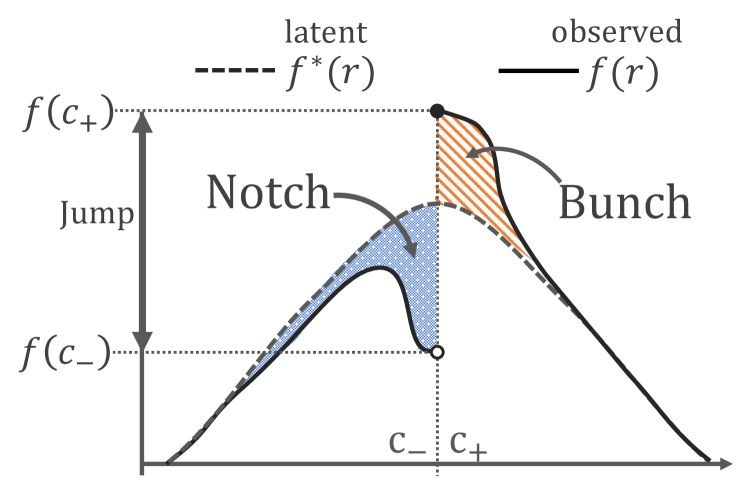
Figure 2.1: Idea of detection with latent and observed density functions.

However, this detection strategy fails if bunches or notches are present on the other side. This failure is illustrated in Figure 2.2. If someone precisely controls $R$ against treatment and others precisely control $R$ in favor of treatment (Figure 2.2 (a)), then the bunches may be canceled out. Furthermore, if someone is precisely selected against treatment and others are precisely selected in favor of treatment (Figure 2.2 (b)), then the notches may be canceled out. Hence, the detection strategy can fail with two-sided incentives for manipulation; some favor treatment but others are against treatment.

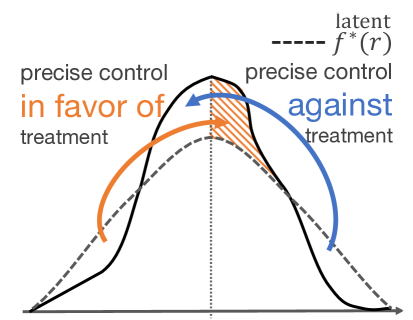
(a) Two-sided bunching fails the detection.

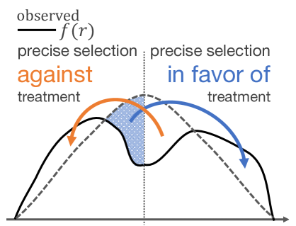
(b) Two-sided notching fails the detection.

Figure 2.2: Examples of detection failures. Detection in Panel (a) fails by bunching at both sides; detection in Panel (b) fails by notching from both sides.

Manipulations in many designs have one-sided incentives. However, the following two designs require closer examination. First, manipulation incentives can be mechanically two-sided. Consider the elections between two major parties, such as the Democrats and Republicans in the US. In such a design, the Democrats favor the treatment where the Democratic Party wins, whereas the Republicans are against the treatment where the Democratic Party wins. In Example 3.2 in Section 3.3, we illustrate our concerns through Lee (2008)’s design. Second, two-sided incentives may arise from multi-dimensional sorting through two-sided matching, such as school matching or labor market matching. Manipulation of this mechanism can disrupt identification and detection. In Section 3.1 and Example 3.1, we detail our concerns and the role of economic theory.

To prevent detection failures, we provide an auxiliary assumption for regulating precise manipulations. As illustrated in Figure 2.2, the detection of precise manipulation depends on who is manipulating for what types of manipulation. Hence, we consider subpopulations based on the latent type of the manipulators and impose the auxiliary restriction on each subpopulation of the manipulators.

We consider three subpopulations of the manipulators. In the toy example, the bribed teachers had complete manipulation that violates both (2.2) and (2.3). Their optimal manipulation $R^{opt}_{i}$ precisely controlled $R_{i}^{opt}=c$ and precisely selected failed students $c-\beta_{i}/\kappa\leq R^{*}_{i}<c$ for manipulation. In some schools, the initial scores $R^{*}_{i}$ are unknown but teachers nevertheless precisely control $R_{i}$ of a few favorite students. For those teachers, precise selection is impossible; hence, their observed-precise manipulation satisfies (2.3) but violates (2.2). In another school, the submitted score $R^{opt}_{i}$ is corrected with an independent random noise $\epsilon_{i}$ to $R_{i}=R_{i}^{opt}+\epsilon_{i}$ to prevent manipulation. For those teachers, precise control is impossible; hence, their latent-precise manipulation satisfies (2.2) but violates (2.3). Table 2.1 summarizes the three types of manipulators that threaten identification.

Table 2.1: Classification of manipulators by their precision

Manipulation is		imprecise control: (2.2) holds
		yes	no
imprecise selection:	yes	$im$ (imprecise)	$op$ (observed-precise)
(2.3) holds	no	$\ell p$ (latent-precise)	$cm$ (complete)

Specifically, we exploit the above classification (imprecise, observed-precise, latent-precise, and complete), formally defined by the following indicator $G$:

Definition 2.1.

Let $G$ be an indicator function that takes one of four values in
$\mathcal{G}\equiv\left\{\begin{gathered}im\text{ (imprecise)},op\text{ (observed-precise)},\ell p\text{ (latent-precise)},cm\text{ (complete)}\end{gathered}\right\}$. For $g\in\{im\mbox{ or }\ell p\}$, the manipulation is an imprecise control; that is,

$$\begin{split}&f(c_{-}|R\neq R^{*},G=g)=f(c_{+}|R\neq R^{*},G=g),\\ &E[Y(d)|R=c_{-},R\neq R^{*},G=g]=E[Y(d)|R=c_{+},R\neq R^{*},G=g],\end{split}$$ (2.5)

and for $g\in\{im\mbox{ or }op\}$, the manipulation is an imprecise selection; that is,

$$\begin{split}&f^{*}(c_{-}|R=R^{*},G=g)=f^{*}(c_{+}|R=R^{*},G=g),\\ &E[Y(d)|R^{*}=c_{-},R=R^{*},G=g]=E[Y(d)|R^{*}=c_{+},R=R^{*},G=g].\end{split}$$ (2.6)

For each $g\in\mathcal{G}$, we impose an auxiliary assumption to regulate precise control and selection. With precise control (op: observed-precise or cm: complete), precise control units should never assign $R$ at $c_{-}$. With precise selection ($\ell$p: latent-precise or cm: complete), precisely selected units should never be manipulated from $R^{*}=c_{+}$:

Assumption 2.2 (One-sided).

Given the classification $G$ in Definition 2.1,

$$0=f(c_{-}|R\neq R^{*},G=g)<f(c_{+}|R\neq R^{*},G=g)\mbox{ for }g\in\{\textit{op},\textit{cm}\};$$

$$P(R=R^{*}|R^{*}=c_{-},G=g)<P(R=R^{*}|R^{*}=c_{+},G=g)=1\mbox{ for }g\in\{\ell p,\textit{cm}\}.$$

Under the auxiliary assumption, precise manipulation is one-sided; if some precise manipulation is in favor of treatment, then no precise manipulation should be against treatment. We emphasize that the above one-sided restriction does not restrict imprecise manipulations. This feature of Assumption 2.2 is a critical difference from the restriction conjectured by McCrary (2008). Appendix B details these differences and provides a counterexample in which the conjectured restriction fails to guarantee detection.

For the desired result, we (i) adjust Assumption 2.1 to accommodate $G$ and (ii) impose that each subpopulation $G=g,g\in\{op,\ell p,cm\}$ always include some manipulators:

Assumption 2.3.

Given an indicator $G$ with the support of $\mathcal{G}$, (i) the latent running variable $R^{*}$ with the density function $f^{*}$ satisfies $f^{*}(c_{+}|G=g)=f^{*}(c_{-}|G=g)$ and $E[Y(d)|R^{*}=c_{+},G=g]=E[Y(d)|R^{*}=c_{-},G=g]$ for each $d\in\{0,1\}$ for any $g\in\mathcal{G}$, and (ii) $P(R\neq R^{*}|G=g)>0$ for $g\in\{op,\ell p,cm\}$.

Under Assumption 2.3, regularity conditions (Assumption A.2 in Appendix A) for the well-defined density and conditional expectations at the boundary, and the auxiliary assumption (Assumption 2.2), the observed density is continuous if and only if all the manipulations are imprecise.

Theorem 2.1.

For a pair $(R,R^{*})$ that satisfies Assumptions 2.2, 2.3, and A.2 for indicator $G$ in Definition 2.1, we have $f(c_{-})\leq f(c_{+})$. Furthermore, the null hypothesis of the density test ($f(c_{-})=f(c_{+})$) holds if and only if $P(G=im)=1$, thereby implying identification.

Proof.

Proof is in Appendix A ∎

Theorem 2.1 also justifies the balance test; that is, the conditional means of covariates are continuous at the cutoff under the null hypothesis of the density test:

Corollary 2.1.

Under the conditions of Theorem 2.1, replacing $Y(d)$ with a pre-determined covariate $W$, $f(c_{-})=f(c_{+})$ implies $E[W|R=c_{+}]=E[W|R=c_{-}]$.

2.3 Validating the bounds with new interpretations

From Theorem 2.1, the continuous density implies identification. In other words, Theorem 2.1 connects the (absence of) discontinuity in the density and the conditional mean for point identification. In this section, we establish the connection between the discontinuity in the density and the conditional mean for partial identification.

In the proof of Theorem 2.1, we show $f(c_{+})-f(c_{-})$ is the sum of a bunch and notch:

$$f(c_{+})-f(c_{-})=\underbrace{f(c_{+};R\neq R^{*},\{op,cm\})}_{\text{bunch}}+\underbrace{f^{*}(c_{-};R\neq R^{*},\{\ell p,cm\})}_{\text{notch}}$$

where the former bunch,

$$f(c_{+};R\neq R^{*},\{op,cm\})\equiv f(c_{+}|R\neq R^{*},G\in\{op,cm\})P(R\neq R^{*},G\in\{op,cm\}),$$

is the inflow of the precisely controlled $R$ into $R=c_{+}$ and the latter notch,

$$f^{*}(c_{-};R\neq R^{*},\{\ell p,cm\})\equiv f^{*}(c_{-}|R\neq R^{*},G\in\{\ell p,cm\})P(R\neq R^{*},G\in\{\ell p,cm\}),$$

is the outflow precisely selected from $R^{*}=c_{-}$ by manipulation. Under the same assumptions, the jump in the conditional mean of $Y(d)$ follows the same interpretation.

Theorem 2.2.

Under the conditions in Theorem 2.1, for each $d\in\{0,1\}$, we have:

$$E[Y(d) |R=c_{+}]f(c_{+})-E[Y(d)|R=c_{-}]f(c_{-})$$

$$= f(c_{+};R\neq R^{*},\{op,cm\})\cdot E[Y(d)|R=c_{+},R\neq R^{*},G\in\{op,cm\}]$$

$$+f^{*}(c_{-};R\neq R^{*},\{\ell p,cm\})\cdot E[Y(d)|R^{*}=c_{-},R\neq R^{*},G\in\{\ell p,cm\}].$$

Proof.

The proof is in Appendix A. ∎

Transforming the expression of Theorem 2.2, the mean at $R=c_{+}$ becomes a convex average of the mean at $R=c_{-}$ and the means of the precise manipulators. Specifically,

$$\begin{split}E[Y(d)|R=c_{+}]=&(1-\tau)\cdot E[Y(d)|R=c_{-}]\\ &+\omega_{op}\cdot E[Y(d)|R=c_{+},R\neq R^{*},G\in\{op,cm\}]\\ &+\omega_{\ell p}\cdot E[Y(d)|R^{*}=c_{-},R\neq R^{*},G\in\{\ell p,cm\}]\end{split}$$ (2.7)

where $\tau\equiv 1-f(c_{-})/f(c_{+})=\omega_{op}+\omega_{\ell p}$, $\omega_{op}=f(c_{+};R\neq R^{*},\{op,cm\})/f(c_{+})$ and $\omega_{\ell p}=f^{*}(c_{-};R\neq R^{*},\{\ell p,cm\}/f(c_{+})$.

This convex average representation (2.7) is the basis for partial identification. For $d=1$, $E[Y(1)|R=c_{+}]$ is observed and the other $E[Y(1)|R=c_{-}]$ is an unobserved target parameter. For $d=0$, $E[Y(0)|R=c_{-}]$ is observed and the other $E[Y(0)|R=c_{+}]$ is an unobserved target parameter. Hence, this representation (2.7) induces the worst-case bounds by replacing the unobserved manipulated moments $E[Y(d)|R=c_{+},R\neq R^{*},G\in\{op,cm\}]$ and $E[Y(d)|R^{*}=c_{-},R\neq R^{*},G\in\{\ell p,cm\}]$ with their worst-case values. Specifically, our representation (2.7) is the foundation of the Gerard et al. (2020) bounds for two different target parameters, $\Gamma_{+}\equiv E[Y(1)-Y(0)|R=c_{+}]$ (Gerard et al., 2016) and $\Gamma_{-}\equiv E[Y(1)-Y(0)|R=c_{-}]$ (Gerard et al., 2020). For both parameters, our representation (2.7) induces the Manski (1989, 1990)-type worst-case bounds:

Assumption 2.4.

For some $(y_{L},y_{U})\in\mathbb{R}^{2}$, $P(y_{L}\leq Y(d)\leq y_{U},d\in\{0,1\})=1$.

Corollary 2.2.

Under the conditions in Theorem 2.2 and Assumption 2.4,

$$(\mu_{+}-y_{U})-(1-\tau)(\mu_{-}-y_{U})\ \leq\ \Gamma_{+}\ \leq\ (\mu_{+}-y_{L})-(1-\tau)(\mu_{-}-y_{L})$$ (2.8)

where $\mu_{+}\equiv E[Y|R=c_{+}],\mu_{-}\equiv E[Y|R=c_{-}]$ and the bounds are sharp. Furthermore,

$$(1-\tau)^{-1}(\mu_{+}-y_{U})-(\mu_{-}-y_{U})\ \leq\ \Gamma_{-}\ \leq\ (1-\tau)^{-1}(\mu_{+}-y_{L})-(\mu_{-}-y_{L}).$$

Proof.

The expressions of the bounds immediately follow from Theorem 2.2. The sharpness of the former bounds follows from Horowitz and Manski (1995). ∎

From these bounds, the auxiliary assumption is the foundation for the Gerard et al. (2016, 2020) bounds. For the former, $\Gamma_{+}\equiv E[Y(1)-Y(0)|R=c_{+}]$, the Manski bounds (2.8) are equivalent to those in the research of Gerard et al. (2016). For the latter, $\Gamma_{-}\equiv E[Y(1)-Y(0)|R=c_{-}]$, we can extend Theorem 2.2 to distribution functions under alternative regularity conditions for the conditional distribution of $Y(d)$. The Lee (2009)-type bounds follow from Lee (2009) via Horowitz and Manski (1995) as:

$$E[Y|R=c_{+},Y\leq Q^{Y|R=c_{+}}_{1-\tau}]-\mu_{-}\leq\Gamma_{-}\leq E[Y|R=c_{+},Y\geq Q^{Y|R=c_{+}}_{\tau}]-\mu_{-}$$ (2.9)

where $Q^{Y|R=c_{+}}_{\tau}$ represents $\tau$th quantile of $Y|R=c_{+}$. The Lee bounds in (2.9) are equivalent to those in Gerard et al. (2020) for $\Gamma_{-}$. We emphasize that these bounds are the immediate consequences of the representation (2.7). Consequently, if the density test is valid, the Gerard et al. (2016, 2020) bounds are valid.

Remark 2.1.

From the construction through (2.7), $\Gamma_{-}$ has a straightforward interpretation when precise selection is absent. Consider the special case of imprecise manipulation for simplicity, namely, $P(G\in\{op,\ell p\})=0$ and $P(R\neq R^{*},G=im)=0$. By applying Assumption 2.2 to precise controls,

$$P(R=R^{*}|R^{*}=c_{-}) =\frac{f^{*}(c_{-}|R=R^{*})P(R=R^{*})}{f^{*}(c)}\ =\ \frac{f(c_{-}|R=R^{*})P(R=R^{*})}{f^{*}(c)}$$

$$=\frac{P(R=R^{*}|R=c_{-})f(c_{-})}{f^{*}(c)}\ =\ \frac{f(c_{-})}{f^{*}(c)},$$

where we use the fact that $f(c_{-}|R\neq R^{*})=0$; consequently,

$$\begin{split}E[Y(d)|R^{*}=c]=&E[Y(d)|R=c_{-}]\left(\frac{f(c_{-})}{f^{*}(c)}\right)\\ &+E[Y(d)|R^{*}=c_{-},R\neq R^{*}]\left(\frac{f^{*}(c)-f(c_{-})}{f^{*}(c)}\right).\end{split}$$ (2.10)

In the absence of imprecise manipulation, no precise selection implies that no one manipulates from $R^{*}=c$. In other words, $P(R=R^{*}|R^{*}=c_{-})=f(c_{-})/f^{*}(c)=1$. Consequently, equality (2.10) becomes

$$E[Y(d)|R^{*}=c]=E[Y(d)|R=c_{-}],\mbox{ for each }d\in\{0,1\},$$

Hence, $\Gamma_{-}=E[Y(1)-Y(0)|R=c_{-}]=E[Y(1)-Y(0)|R^{*}=c]$ that is the ATE for students at $R^{*}=c$. If imprecise manipulation is allowed, $\Gamma_{-}$ is the ATE for students at $R^{*}=c$ by adding students who manipulated $R$ to $R=c_{+}$ by chance, and excluding students who manipulated from $R^{*}=c_{-}$ without knowing $R^{*}<c$. This interpretation of $\Gamma_{-}$ is consistent with Gerard et al. (2020) on $E[Y(1)-Y(0)|M=0]$, where $M=1$ is the always-assigned, whose $R$ is always above the cutoff.

Remark 2.2.

When precise control is absent, $\Gamma_{+}$ also has a straightforward interpretation. Consider again the special case of imprecise manipulation. By applying Assumption 2.2 for precise selection,

$$P(R=R^{*}|R=c_{+})= \frac{f(c_{+}|R=R^{*})P(R=R^{*})}{f(c_{+})}\ =\ \frac{f^{*}(c_{+}|R=R^{*})P(R=R^{*})}{f(c_{+})}$$

$$= \frac{P(R=R^{*}|R^{*}=c_{+})f^{*}(c)}{f(c_{+})}\ =\ \frac{f^{*}(c)}{f(c_{+})}$$

where we use the fact that $P(R=R^{*}|R^{*}=c_{+})=1$. As a result,

$$\begin{split}E[Y(d)|R=c_{+}]=&\left(\frac{f^{*}(c)}{f(c_{+})}\right)E[Y(d)|R^{*}=c]\\ &+\left(\frac{f(c_{+})-f^{*}(c)}{f(c_{+})}\right)E[Y(d)|R=c_{+},R\neq R^{*}].\end{split}$$ (2.11)

In the absence of imprecise manipulation, no precise control implies that no one manipulates into $R=c_{+}$. In other words, anyone at $R=c_{+}$ never manipulated, $P(R=R^{*}|R=c_{+})=f^{*}(c)/f(c_{+})=1$. Consequently, the equality (2.11) becomes

$$E[Y(d)|R=c_{+}]=E[Y(d)|R^{*}=c],\mbox{ for each }d\in\{0,1\}.$$

Hence, $\Gamma_{+}=E[Y(1)-Y(0)|R=c_{+}]$ is the ATE for the students at $R^{*}=c$. If imprecise manipulation is allowed, $\Gamma_{+}$ is the ATE for students at $R^{*}=c$ by adding students who manipulated $R$ to $R=c_{+}$ by chance, and excluding students who manipulated from $R^{*}=c_{-}$ without knowing $R^{*}<c$. This interpretation of $\Gamma_{+}$ is novel. Hence, the new interpretation of $\Gamma_{+}$ enriches the use of the other bounds by Gerard et al. (2016).

Remark 2.3.

Precise control without precise selection is possible when the test score $R^{*}$ is unknown and there is no systematic attrition, but some students obtain a passing grade $R\geq c$, regardless of the score $R^{*}$ they initially received. Precise selection without precise controls is also plausible. For example, precise selection occurs when we observe all treated students but only a self-selected sample of control students. Another example is the second home visit example (Gerard et al., 2020, Appendix D.). In this example, a poverty score survey, $R^{*}$, determines eligibility for a program, but a household may claim a second home visit to correct errors in the initial survey. If the claim for a second home visit is made only after learning that they are ineligible, $R^{*}<c$, then this results in precise selection. If the manipulating households know the cutoff and $R^{*}$, then the manipulation can also be precisely controlled. Nevertheless, if neither surveyors nor households know the cutoff, precise control is impossible.

Remark 2.4.

Combining the expressions (2.10) and (2.11) yields the expression of Theorem 2.2 in the special case. The general case is derived in the Appendix proof.

3 Recommended procedures and case studies

3.1 When do our concerns apply?

Our analysis reveals two concerns regarding RD practices: The current identification argument is insufficient, and diagnostic tests may not detect identification failures. We summarize when these concerns apply in practice.

First, the typical identification argument is insufficient. Lee and Lemieux (2010) claim that local randomization holds if “individuals do not have precise control over the assignment variable” (page. 295). Also in the latest textbook exposition, “if units lack the ability to precisely manipulate the score value they receive, there should be no systematic differences between units with similar values of the score.” (Cattaneo et al., 2023, page. 89). Empirical studies follow the same argument. However, such arguments are insufficient for identification.

We demonstrate that identification could fail without precise control. Identification can fail without any control over the value of the observed running variable or final assignment status. If the likelihood of manipulation differs around the cutoff value, identification can fail. Hence, identification can fail from any attempt to control the final assignment status. If there is any sample selection involving the treatment assignment, one should be concerned about its identification.

Second, no studies have provided the auxiliary assumption for the diagnostic tests to detect precise manipulations. We show that the manipulation incentive must be one-sided to detect manipulations. If all units prefer the treatment and avoid the control, our one-sided restriction is appropriate. Most designs with favorable policies have a one-sided incentive to favor treatment when there are no expected side effects.

However, two types of design concerns exist. The first type of concerning design is when the units may have mechanically two-sided incentives. For example, electoral RD designs are concerning when the running variable is the vote-share gap between the two major parties. In the US election, if a Democratic candidate is capable of having precise manipulation in one district, then a Republican candidate should also be capable of having precise manipulation in another district. Consequently, precise manipulations are likely to favor both high and low values of the running variable. See Example 3.2 for a further illustration in the context of Lee (2008) and how to mitigate this issue.

The second type of concerning design is when the design is from two-sided matching mechanisms such as school matching. For example, Abdulkadiroğlu, Angrist, Narita, and Pathak (2022) exploit the tie-breaking rule for test scores in an RD design. In some school matching mechanisms, schools sort students using a tie breaker, such as test scores. Tie breakers themselves may be locally random, but students favor different schools for different reasons in two-sided matching. Some students favor prestigious schools with higher tie-breaking thresholds, whereas others favor less prestigious schools for other amenities. If students or schools submit a particular preference order to manipulate the matching system, these manipulations are precise and their motivations are two-sided.

Economic theory may help justify restrictions because the manipulation of the mechanism has been well studied. As summarized by Kojima and Pathak (2009), in the Gale-Sharpley mechanism, schools may have manipulation incentives, whereas students do not (Dubins and Freedman, 1981; Roth, 1982). In a small market, schools can manipulate assignments by falsely submitting their capacity constraints (Sönmez, 1997); however, such manipulation is difficult in a large market (Kojima and Pathak, 2009). In a large market, manipulation is less of a concern in the Gale-Sharpley mechanism. Nevertheless, any manipulation (in our sense) after the assignment of the mechanism remains concerning. For example, precise selection still arises from attrition of the outcome variable. See Example 3.1 for a case study on this attrition issue.

3.2 How should empirical researchers deal with our concerns?

This study offers solutions to the aforementioned concerns. We recommend the following three steps. First, specify the latent $R^{*}$. Second, categorize any manipulations that deviate the observed $R$ from the latent $R^{*}$. Third, justify the one-sided restriction or take measures to justify it. Following these three steps guarantees the partial identification results of Gerard et al. (2016, 2020).

First, we specify the latent running variable $R^{*}$. For most designs with an artificial policy cutoff, latent $R^{*}$ is the running variable that would be realized if the policy of interest were absent. If the policy were absent, then nobody would care about being on either side of the cutoff; hence, latent $R^{*}$ satisfies local randomization (Assumption 2.1). Again, we emphasize that neither knowledge nor shape restrictions of the distribution of $R^{*}$ are required. Consequently, specifying $R^{*}$ does not impose any restrictions on the design. With latent $R^{*}$, the manipulation is unambiguously defined.

Second, we list all the possible manipulations to assess their precision. Any control over the realized score is concerning because it can be a precise control of the manipulated $R$ (violation of (2.2)). Any sample selection from either side of the cutoff is also concerning because it can be a precise selection (violation of (2.3)). If neither of the two precise manipulations is possible, then the point estimand equals the ATE at $R=c$ (Proposition 2.1). For example, if the cutoff $c$ is unknown to all stakeholders, then most precise manipulations are impossible; nevertheless, sample selection remains a concern for precise selection. See Example C.1 in Appendix C for an example of this situation.

Finally, we justify the diagnostic test whenever precise manipulations are concerning. To test whether precise manipulations are present, such manipulations must satisfy a one-sided restriction (Assumption 2.2). We emphasize that identification and detection are valid with two-sided incentives for imprecise manipulation.

Sometimes, the one-sided restriction is difficult to justify because of two-sided incentives. Economic theory may help justify this restriction as demonstrated in Section 3.1. Otherwise, we may modify the definition of the running variable or take a subsample using pre-treatment covariates. See Example 3.2 for a remedy of the former approach.

3.3 Case studies

We illustrate the recommended practices in two case studies. Appendix C provides further case studies and a review of past partial identification strategies.

Example 3.1 (A Romanian secondary school matching study).

Pop-Eleches and Urquiola (2013a) study the effect of being accepted into a better school through a school matching system for Romanian secondary schools. Their study follows an RD design in which precise control is difficult, but precise selection is likely.

In Romania, secondary education is mandatory and every middle school student takes a nationwide exam for transition. Each student receives a transition score, which is the average of the exam score and grade point average. Given the transition score, students submit their school preferences, while the transition score determines the final assignment of students to each school. Better schools are those with higher average transition scores among the accepted students. They study the effect of being accepted into a better school on their future Baccalaureate grades for college admission.

First, we specify the latent transition score $R^{*}$. For each school $j$, the cutoff is the lowest transition score $c_{j}$ among the accepted students. Hence, the realized score $R$ is the transition score minus the cutoff value $c_{j}$. Consequently, the cutoff value is normalized $0$. The latent score $R^{*}$ is the transition score that students would receive if the transition score were irrelevant to the matching.

Second, we list all the concerning manipulations given the notion of $R^{*}$. According to Pop-Eleches and Urquiola (2013a), the transition score is the sole criterion for ranking students, given their submitted preferences. A computerized system at the Ministry of Education governs the assignment based on the transition score; additionally, the assignment is endogenous to satisfy the capacity constraint of each school. Consequently, precise control is challenging because students must manipulate the matching mechanism to control their final assignment status. The same argument applies to precise selection through the matching mechanism. However, precise selection is also possible from selective attrition because not everyone takes the Baccalaureate exam. Pop-Eleches and Urquiola (2013a) omitted students with missing Baccalaureate grades. Hence, the selective attrition of this outcome variable induces (unintentional) precise selection.

Finally, we assess the one-sided restriction. The assignment is based on two-sided matching: students submit their preferences and the matching mechanism assigns students based on their transition scores. In principle, a two-sided manipulation is a concern. Some students may favor better schools based on their scores, while others may favor non-better schools with other amenities. Hence, it is critical to argue that precise manipulation through the mechanism is difficult. Fortunately, manipulation of the mechanism appears to be challenging. Furthermore, the theory of the underlying mechanism helps validate the design. In fact, “Under this set up students have incentives to truthfully reveal their preference rankings.” (page. 1295, Pop-Eleches and Urquiola, 2013a) because serial dictatorship is strategic-proof (Svensson, 1999). For the precise selection from the attrition, students who did not take the Baccalaureate exam would have taken the exam if they had been accepted at a better school because of peer effects. If the students dropped out of the sample because of the assignment, they must have dropped only from the rejected side and not the accepted side. Other drop-outs are the imprecise manipulators because they would have dropped out in both schools. For this reason, we argue that selective attrition is one-sided and the density test is valid.

Simultaneously, the bounds are valid under the one-sided restriction. Among the two parameters, $\Gamma_{+}$ has an interpretation closer to $E[Y(1)-Y(0)|R^{*}=c]$ because precise control is limited. Nevertheless, the grade is a continuous variable. Hence, we recommend constructing a binary variable for $\Gamma_{+}$ or using Lee (2009) bounds for $\Gamma_{-}$.

We characterize the consequences of precise selection by using the two subsamples studied by Pop-Eleches and Urquiola (2013a) using their data Pop-Eleches and Urquiola (2013b). On the one hand, the “Top tercile” subsample (Table 5 Panel B in Pop-Eleches and Urquiola, 2013a) represents the pool of selective schools. Hence, most students take the Baccalaureate exam in either better or worse schools. The density test statistic $1-\tau$ is close to $1$, as $\tau$ has a value of $0.022$. This continuous density is consistent with the effect of better schools on the probability of taking the Baccalaureate exam, which is close to zero (the magnitude was $0.003$, with a standard error of $0.002$). Because the $\tau$ statistic is close to zero, the point estimation remains valid. On the other hand, the other subsample of “towns with only two schools” (Table 5, Panel F) is composed of students from smaller towns with only two schools as their options. Unlike the selective school sample, attending a better school was critical to attrition. The $\tau$ statistic was $0.309$, indicating that the observed students were 30% less just below the cutoff, rather than just above the cutoff, in the worst case. Consequently, point identification may be invalid. Furthermore, the bounds may be uninformative because of their wide length given the large $\tau$ estimate.

Example 3.2 (US house of representatives).

Another example is the well-known voting RD study by Lee (2008) and a follow-up study by Caughey and Sekhon (2011a). Manipulations in voting RD design can take the form of campaigns or voting fraud. In their study, we consider that precise selection was difficult but precise control was possible. Furthermore, the manipulation incentive is mechanically two-sided.

First, we specify the latent vote share gap $R^{*}$. The leading candidate for $R^{*}$ is the counterfactual vote share without campaign efforts or electoral misconduct. Without those manipulations, no one can predict the voting results; hence $R^{*}$ is locally random.

Second, we consider possible manipulations given $R^{*}$. Empirical researchers rationalize voting RD designs based on their inability to predict results. This inability serves as strong evidence for the absence of precise selection. If all the voting results are observed and no one knows the voting results before the election, the precise selection is impossible. Especially, precise manipulation through campaign efforts is unrealistic (de la Cuesta and Imai, 2016). Nevertheless, post-election sorting such as voting fraud is possible. The post-election sorting overrides the election results; hence, identification may be vulnerable to precise control.

Finally, we need to justify the diagnostic test. Lee (2008) studies the incumbent margin in the probability of winning the election for the US House of Representatives. His definition of the score is the Democratic candidates’ vote-share margin. Caughey and Sekhon (2011a) argue that the incumbents in the previous election have the power to manipulate the electoral results, while both Democrats and Republicans can be the incumbents. As a result, Caughey and Sekhon (2011a) propose an alternative running variable, the vote-share margin of previous incumbents.

Given our manipulation-robust designs, we agree with their concerns because precise manipulation is possible from either Democratic or Republican incumbents. Hence, the one-sided restriction (Assumption 2.2) may not hold. The alternative running variable (i.e., the previous incumbents’ vote-share margin) is a reasonable remedy. For example, the one-sided restriction is justified if the voting fraud is possible only for the previous incumbents who have the current control of the district.

Given the alternative definition of the score, Caughey and Sekhon (2011a) document a possible discontinuity at zero with 0.5%-wide histogram plots. We revisited this null hypothesis of the density test using their data, Caughey and Sekhon (2011b). Using the estimator of Cattaneo et al. (2020b), we find no strong evidence of discontinuity, given the optimal bandwidth selection with a local polynomial estimator. Figure 3.3 (b) shows the density test using the local linear estimates proposed by Cattaneo et al. (2020b). The $\tau$ statistic is positive but the jump is insignificant at the $5\%$ level. Interestingly, the jump is insignificant but negative for the original running variable (Figure 3.3 (a)).

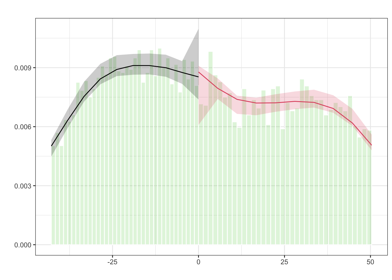
(a) Negative $\tau$ for the original $R$.

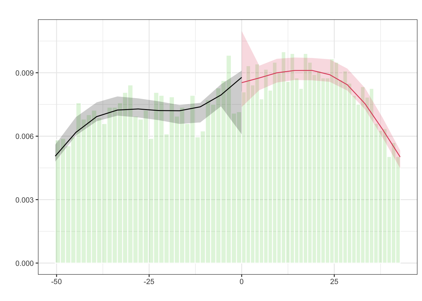
(b) Positive small $\tau$ for the alternative $R$.

Figure 3.3: Density plots for two definitions of the running variable from Lee (2008) (source: Caughey and Sekhon, 2011a) using rddensity by Cattaneo et al. (2020b)

Consequently, we conclude that the alternative running variable is more reasonable than the original; nevertheless, we do not find evidence of precise control at the cutoff. This finding is consistent with follow-up studies, such as that conducted by de la Cuesta and Imai (2016), who mention that the balance tests of Caughey and Sekhon (2011a) are subject to the multiple testing problem. See Fusejima, Ishihara, and Sawada (2023) for an alternative solution to the multiple testing problem in the diagnostic tests.

4 Conclusion

RD identification is valid when the design is as good as randomization locally at the cutoff. However, practical RD designs are not randomized control trials. Notably, individuals may manipulate the running variable. Nevertheless, justifying identification is challenging because manipulation is implicit in the definition of the existing identification condition, namely, local randomization.

Following McCrary (2008), we define manipulation as the deviation of the observed running variable from a latent running variable that is unobserved, counterfactual, and locally randomized. The latent running variable is a running variable that would be realized if the policy of interest were absent. Consider the example of a qualification exam in which a test score determines qualification based on whether it exceeds a cutoff. In this example, a practice exam score is a candidate for the latent running variable because the practice exam has no influence on the qualification. Manipulation includes students cheating during the exam, teachers altering the scores of failing students, teachers offering exam retakes for failing students, as well as analysts selecting a subsample of a non-missing dependent variable. In practice, one must argue that these manipulations do not disrupt identification or that diagnostic tests can detect them.

In Section 2.1, we examine a primitive condition that guarantees identification without the explicit randomization of the observed running variable. Our identification conditions included an explicit pair of restrictions on manipulation. First, no manipulation should precisely control the manipulated running variable. Second, manipulation should not involve sample selection precisely based on the latent running variable. The former restriction for manipulation is well-known as imprecise control, whereas the latter is the overlooked novel concept of imprecise selection. Consequently, we warn that empirical researchers should justify identification with imprecise control and imprecise selection because the latter may fail under the former.

Furthermore, in Section 2.2, we present the first auxiliary assumption that guarantees that diagnostic tests can detect manipulations. Under the proposed auxiliary assumption, we show that the null hypothesis of the popular density test (McCrary, 2008) implies identification. Conversely, the density test should not be applied to designs with two-sided incentives that violate the auxiliary condition. We caution empirical researchers to pay special attention to designs with manipulation incentives for the treatment as well as for the control when applying the density test. The design of a two-sided matching mechanism is also concerning, as the manipulation of the matching mechanism has been a concern in mechanism design. Nevertheless, economic theories may help limit and regulate possible manipulations to justify identification and detection.

Finally, in Section 2.3, we demonstrate that the same auxiliary assumption justifies the partial identification results of Gerard et al. (2020). We provide a convex average representation of the target moments to derive the worst-case bounds naturally. Notably, the target parameters in the research of Gerard et al. (2020) and Gerard et al. (2016) have straightforward interpretations under our conditions. Consequently, our results enhance the usefulness of Gerard et al. (2020) and Gerard et al. (2016) ’s bounds.

The practical implications are summarized in Section 3, followed by two case studies. Reviewing the former study by Pop-Eleches and Urquiola (2013a), we demonstrated that economic theory helps justify identification and detection. Nevertheless, we illustrate the consequences of selective attrition as manipulation with precise selection. Reviewing the latter studies by Lee (2008) and Caughey and Sekhon (2011a), we illustrate a remedy for an RD design that may not satisfy the auxiliary assumption. In Appendix C, we present additional case studies to illustrate the manipulation concerns (Examples C.1 and C.2) and past usage of bounds (Example C.3) before Gerard et al. (2020).

However, several issues remain unresolved. First, the bounds are not informative when the jump in density is sufficiently large. For our analysis, we have no shape restriction on $R^{*}$; however, shape restrictions on $R^{*}$ may improve the informativeness of the bounds, in addition to our manipulation-robust RD design. Second, we may improve the inference of the bounds because it faces the challenge of using density ratio estimates. When the density ratio estimation contains noise, the confidence interval may be too wide to be informative. Third, for some applications, the distribution of $R^{*}$ may be known or its proxy variable may be available. We do not consider the consequences of the additional information for the diagnostic tests and identification; however, this additional information may improve testing and identification. Fourth, the predetermined covariates may have alternative uses based on our analysis. In addition to the balance or placebo test, Frölich and Huber (2019) propose a method with a multi-dimensional non-parametric estimation; further, Calonico, Cattaneo, Farrell, and Titiunik (2019) develop an easy-to-implement augmentation; moreover, Noack, Olma, and Rothe (2021) consider flexible and efficient estimation including machine-learning devices; additionally, several studies such as those conducted by Kreiss and Rothe (2022) and Arai, Otsu, and Seo (2021b) explore augmentation with high-dimensional covariates. Nevertheless, covariates are rarely used to adjust for a possible identification failure. Hence, our results may suggest an alternative use of covariates to correct for identification failure. Finally, we focus on RD designs with a scalar running variable because our analysis may not be trivial with a multi-dimensional running variable $R$. Another promising direction would be to extend our analysis to RD designs with multiple cutoff values. For multiple-cutoff RD designs, Cattaneo, Keele, Titiunik, and Vazquez-Bare (2016) propose a pooling parameter and its implementation, and Cattaneo, Keele, Titiunik, and Vazquez-Bare (2021) consider an extrapolation method to recover the external validity of the estimates. Developing a conceptual and practical recommendation for manipulation-robust design with multiple cutoffs is a future issue to be explored.

Appendix A Regularity conditions and proofs

Assumption A.1 (Regularity conditions).

(i) The following conditional density functions exist: $f^{*}(r^{*}|R\neq R^{*})$ and $f(r|R^{*}=r^{*},R\neq R^{*})$, which are bounded and have left and right limits—i.e.,

$$f^{*}(c_{-}|R=R^{*})\ \equiv \ \lim_{r^{*}\uparrow c}f^{*}(r^{*}|R=R^{*}),$$

$$f^{*}(c_{+}|R=R^{*})\ \equiv \ \lim_{r^{*}\downarrow c}f^{*}(r^{*}|R=R^{*}),$$

$$f(c_{-}|R^{*}=r^{*},R\neq R^{*})\ \equiv \ \lim_{r\uparrow c}f(r|R^{*}=r^{*},R\neq R^{*}),\text{ and }$$

$$f(c_{+}|R^{*}=r^{*},R\neq R^{*})\ \equiv \ \lim_{r\downarrow c}f(r|R^{*}=r^{*},R\neq R^{*})\mbox{ exist}.$$

(ii) For $d\in\{0,1\}$, the following conditional expectations exist: $E[Y(d)|R=r,R^{*}=r^{*},R\neq R^{*}]$, which are bounded and have left and right limits—i.e.,

$$E[Y(d)|R^{*}=c_{-},R=R^{*}]\ \equiv\ \lim_{r^{*}\uparrow c}E[Y(d)|R^{*}=r^{*},R=R^{*}],$$

$$E[Y(d)|R^{*}=c_{+},R=R^{*}]\ \equiv\ \lim_{r^{*}\downarrow c}E[Y(d)|R^{*}=r^{*},R=R^{*}],$$

$$E[Y(d)|R=c_{-},R^{*}=r^{*},R\neq R^{*}]\equiv\ \lim_{r\uparrow c}E[Y(d)|R=r,R^{*}=r^{*},R\neq R^{*}],\text{ and }$$

$$E[Y(d)|R=c_{+},R^{*}=r^{*},R\neq R^{*}]\equiv\ \lim_{r\downarrow c}E[Y(d)|R=r,R^{*}=r^{*},R\neq R^{*}]\mbox{ exist}.$$

(iii) The density values $f(c_{-})\equiv\lim_{r\uparrow c}f(r)$, $f(c_{+})\equiv\lim_{r\downarrow c}f(r)$ are strictly positive.

Assumption A.2 (Regularity conditions with $G$).

(i) For $g\in\mathcal{G}$, the following conditional density functions exist: $f^{*}(r^{*}|R\neq R^{*},G=g)$ and $f(r|R^{*}=r^{*},R\neq R^{*},G=g)$, which are bounded and have left and right limits—i.e.,

$$f^{*}(c_{-}|R=R^{*},G=g)\ \equiv \ \lim_{r^{*}\uparrow c}f^{*}(r^{*}|R=R^{*},G=g),$$

$$f^{*}(c_{+}|R=R^{*},G=g)\ \equiv \ \lim_{r^{*}\downarrow c}f^{*}(r^{*}|R=R^{*},G=g),$$

$$f(c_{-}|R^{*}05=r^{*},R\neq R^{*},G=g)\ \equiv \ \lim_{r\uparrow c}f(r|R^{*}=r^{*},R\neq R^{*},G=g),\text{ and }$$

$$f(c_{+}|R^{*}=r^{*},R\neq R^{*},G=g)\ \equiv \ \lim_{r\downarrow c}f(r|R^{*}=r^{*},R\neq R^{*},G=g)\mbox{ exist}.$$

(ii) For $d\in\{0,1\}$ and $g\in\mathcal{G}$, the following conditional expectations exist: $E[Y(d)|R=r,R^{*}=r^{*},R\neq R^{*},G=g]$, which are bounded and have left and right limits—i.e.,

$$E[Y(d)|R^{*}=c_{-},R=R^{*},G=g]\ \equiv\ \lim_{r^{*}\uparrow c}E[Y(d)|R^{*}=r^{*},R=R^{*},G=g],$$

$$E[Y(d)|R^{*}=c_{+},R=R^{*},G=g]\ \equiv\ \lim_{r^{*}\downarrow c}E[Y(d)|R^{*}=r^{*},R=R^{*},G=g],$$

$$E[Y(d)|R=c_{-},R^{*}=r^{*},R\neq R^{*},G=g]$$

$$\hskip 86.72377pt\equiv\ \lim_{r\uparrow c}E[Y(d)|R=r,R^{*}=r^{*},R\neq R^{*},G=g],\text{ and }$$

$$E[Y(d)|R=c_{+},R^{*}=r^{*},R\neq R^{*},G=g]$$

$$\hskip 86.72377pt\equiv\ \lim_{r\downarrow c}E[Y(d)|R=r,R^{*}=r^{*},R\neq R^{*},G=g]\mbox{ exist}.$$

(iii) The density values $f(c_{-})\equiv\lim_{r\uparrow c}f(r)$, $f(c_{+})\equiv\lim_{r\downarrow c}f(r)$, and $f^{*}(c|G=g)$ are strictly positive for $g\in\{im,op,\ell p,cm\}$.

Lemma A.1.

Suppose that Assumptions 2.2, 2.3, and A.2 hold true. We define

$$w_{1} \equiv f^{*}(c|R=R^{*},G\in\{im,op\})P(R=R^{*}|G\in\{im,op\}),$$

$$w_{2} \equiv f(c|R\neq R^{*},G=im)P(R\neq R^{*},G=im|G\in\{im,op\}),$$

$$w_{3} \equiv f(c_{+}|R\neq R^{*},G=op)P(R\neq R^{*},G=op|G\in\{im,op\}).$$

Then, we have

$$f(c_{-}|G\in\{im,op\}) = w_{1}+w_{2},$$

$$f(c_{+}|G\in\{im,op\}) = w_{1}+w_{2}+w_{3}.$$

Furthermore, we obtain

$$E[Y(d)|R=c_{-},G\in\{im,op\}]$$

$$= E[Y(d)|R^{*}=c,R=R^{*},G\in\{im,op\}]\left(\frac{w_{1}}{f(c_{-}|G\in\{im,op\})}\right)$$

$$+E[Y(d)|R=c,R\neq R^{*},G=im]\left(\frac{w_{2}}{f(c_{-}|G\in\{im,op\})}\right)$$

and

$$E[Y(d)|R=c_{+},G\in\{im,op\}]$$

$$= E[Y(d)|R^{*}=c,R=R^{*},G\in\{im,op\}]\left(\frac{w_{1}}{f(c_{+}|G\in\{im,op\})}\right)$$

$$+E[Y(d)|R=c,R\neq R^{*},G=im]\left(\frac{w_{2}}{f(c_{+}|G\in\{im,op\})}\right)$$

$$+E[Y(d)|R=c_{+},R\neq R^{*},G=op]\left(\frac{w_{3}}{f(c_{+}|G\in\{im,op\})}\right).$$

Proof.

We observe that

$$f(c_{-}|G\in\{im,op\}) = f^{*}(c|R=R^{*},G\in\{im,op\})P(R=R^{*}|G\in\{im,op\})$$

$$+f(c|R\neq R^{*},G=im)P(R\neq R^{*},G=im|G\in\{im,op\}),$$

where we use $f(c_{-}|R\neq R^{*},G=op)=0$. Hence, we obtain $f(c_{-}|G\in\{im,op\})=w_{1}+w_{2}$. Similarly, we obtain $f(c_{+}|G\in\{im,op\})=w_{1}+w_{2}+w_{3}$.

Next, we consider the expressions of $E[Y(d)|R=c_{-},G\in\{im,op\}]$ and $E[Y(d)|R=c_{+},G\in\{im,op\}]$. As $f(c_{-}|R\neq R^{*},G=op)=0$, we have

$$P(R\neq R^{*}|R=c_{-},G=op)=\frac{f(c_{-}|R\neq R^{*},G=op)P(R\neq R^{*}|G=op)}{f(c_{-}|G=op)}=0.$$

Hence, we obtain

$$E[Y(d)|R=c_{-},G\in\{im,op\}]$$

$$= E[Y(d)|R=c_{-},R=R^{*},G\in\{im,op\}]P(R=R^{*}|R=c_{-},G\in\{im,op\})$$

$$+E[Y(d)|R=c_{-},R\neq R^{*},G=im]P(R\neq R^{*},G=im|R=c_{-},G\in\{im,op\}).$$

Here, we observe that

$$P(R=R^{*}|R=c_{-},G\in\{im,op\})$$

$$= \frac{f(c_{-}|R=R^{*},G\in\{im,op\})P(R=R^{*}|G\in\{im,op\})}{f(c_{-}|G\in\{im,op\})}$$

$$= \frac{f^{*}(c|R=R^{*},G\in\{im,op\})P(R=R^{*}|G\in\{im,op\})}{f(c_{-}|G\in\{im,op\})},$$

which implies that

$$P(R=R^{*},G=im|R=c_{-},G\in\{im,op\})=\frac{w_{1}}{f(c_{-}|G\in\{im,op\})}.$$

From similar calculations, we obtain the expression for $E[Y(d)|R=c_{-},G\in\{im,op\}]$. Similarly, we obtain the expression for $E[Y(d)|R=c_{+},G\in\{im,op\}]$. ∎

Lemma A.2.

Suppose that Assumptions 2.2, 2.3, and A.2 hold true. We define

$$\tilde{w}_{1} \equiv f^{*}(c_{-}|R=R^{*},G\in\{\ell p,cm\})P(R=R^{*}|G\in\{\ell p,cm\}),$$

$$\tilde{w}_{2} \equiv f^{*}(c_{-}|R\neq R^{*},G\in\{\ell p,cm\})P(R\neq R^{*}|G\in\{\ell p,cm\})$$

$$\tilde{w}_{3} \equiv f(c|R\neq R^{*},G=\ell p)P(R\neq R^{*},G=\ell p|G\in\{\ell p,cm\}),$$

$$\tilde{w}_{4} \equiv f(c_{+}|R\neq R^{*},G=cm)P(R\neq R^{*},G=cm|G\in\{\ell p,cm\}).$$

Then, we have

$$f(c_{-}|G\in\{\ell p,cm\}) = \tilde{w}_{1}+\tilde{w}_{3},$$

$$f(c_{+}|G\in\{\ell p,cm\}) = \tilde{w}_{1}+\tilde{w}_{2}+\tilde{w}_{3}+\tilde{w}_{4},$$

Furthermore, we obtain

$$E[Y(d)|R=c_{-},G\in\{\ell p,cm\}]$$

$$= E[Y(d)|R^{*}=c,G\in\{\ell p,cm\}]\left(\frac{\tilde{w}_{1}+\tilde{w}_{2}}{f(c_{-}|G\in\{\ell p,cm\})}\right)$$

$$-E[Y(d)|R^{*}=c_{-},R\neq R^{*},G\in\{\ell p,cm\}]\left(\frac{\tilde{w}_{2}}{f(c_{-}|G\in\{\ell p,cm\})}\right)$$

$$+E[Y(d)|R=c,R\neq R^{*},G=\ell p]\left(\frac{\tilde{w}_{3}}{f(c_{-}|G\in\{\ell p,cm\})}\right)$$

and

$$E[Y(d)|R=c_{+},G\in\{\ell p,cm\}]$$

$$= E[Y(d)|R^{*}=c,G\in\{\ell p,cm\}]\left(\frac{\tilde{w}_{1}+\tilde{w}_{2}}{f(c_{+}|G\in\{\ell p,cm\})}\right)$$

$$+E[Y(d)|R=c,R\neq R^{*},G=\ell p]\left(\frac{\tilde{w}_{3}}{f(c_{+}|G\in\{\ell p,cm\})}\right)$$

$$+E[Y(d)|R=c_{+},R\neq R^{*},G=cm]\left(\frac{\tilde{w}_{4}}{f(c_{+}|G\in\{\ell p,cm\})}\right).$$

Proof.

We observe that

$$f(c_{-}|G\in\{\ell p,cm\})$$

$$= f^{*}(c_{-}|R=R^{*},G\in\{\ell p,cm\})P(R=R^{*}|G\in\{\ell p,cm\})$$

$$+f(c|R\neq R^{*},G=\ell p)P(R\neq R^{*},G=\ell p|G\in\{\ell p,cm\}),$$

where we use $f(c_{-}|R\neq R^{*},G=\ell p)=f(c_{+}|R\neq R^{*},G=\ell p)$ and $f(c_{-}|R\neq R^{*},G=cm)=0$. Thus, we obtain $f(c_{-}|G\in\{\ell p,cm\})=\tilde{w}_{1}+\tilde{w_{3}}$. Similarly, we observe that

$$f(c_{+}|G\in\{\ell p,cm\})$$

$$= f^{*}(c_{+}|R=R^{*},G\in\{\ell p,cm\})P(R=R^{*}|G\in\{\ell p,cm\})$$

$$+f(c|R\neq R^{*},G=\ell p)P(R\neq R^{*},G=\ell p|G\in\{\ell p,cm\})$$

$$+f(c_{+}|R\neq R^{*},G=cm)P(R\neq R^{*},G=cm|G\in\{\ell p,cm\}),$$

where

$$f^{*}(c_{+}|R=R^{*},G\in\{\ell p,cm\})P(R=R^{*}|G\in\{\ell p,cm\})$$

$$= P(R=R^{*}|R^{*}=c_{+},G\in\{\ell p,cm\})f^{*}(c|G\in\{\ell p,cm\})=f^{*}(c|G\in\{\ell p,cm\}).$$

Because $\tilde{w}_{1}+\tilde{w}_{2}=f^{*}(c_{-}|G\in\{\ell p,cm\})=f^{*}(c|G\in\{\ell p,cm\})$, we obtain $f(c_{+}|G\in\{\ell p,cm\})=\tilde{w}_{1}+\tilde{w}_{2}+\tilde{w}_{3}+\tilde{w}_{4}$.

We consider the expression of $E[Y(d)|R=c+,G\in\{\ell p,cm\}]$. We observe that

$$E[Y(d)|R=c_{+},G\in\{\ell p,cm\}]$$

$$= E[Y(d)|R^{*}=c_{+},R=R^{*},G\in\{\ell p,cm\}]P(R=R^{*}|R=c_{+},G\in\{\ell p,cm\})$$

$$+E[Y(d)|R=c_{+},R\neq R^{*},G=\ell p]P(R\neq R^{*},G=\ell p|R=c_{+},G\in\{\ell p,cm\})$$

$$+E[Y(d)|R=c_{+},R\neq R^{*},G=cm]P(R\neq R^{*},G=cm|R=c_{+},G\in\{\ell p,cm\}),$$

where it follows from $P(R=R^{*}|R^{*}=c_{+},G\in\{\ell p,cm\})=1$ that

$$E[Y(d)|R^{*}=c_{+},R=R^{*},G\in\{\ell p,cm\}] = E[Y(d)|R^{*}=c_{+},G\in\{\ell p,cm\}]$$

$$= E[Y(d)|R^{*}=c,G\in\{\ell p,cm\}].$$

Here, we observe that

$$P(R=R^{*}|R=c_{+},G\in\{\ell p,cm\})$$

$$= \frac{f^{*}(c_{+}|R=R^{*},G\in\{\ell p,cm\})P(R=R^{*}|G\in\{\ell p,cm\})}{f(c_{+}|G\in\{\ell p,cm\})}$$

$$= \frac{P(R=R^{*}|R^{*}=c_{+},G\in\{\ell p,cm\})f^{*}(c|G\in\{\ell p,cm\})}{f(c_{+}|G\in\{\ell p,cm\})}$$

$$= \frac{f^{*}(c|G\in\{\ell p,cm\})}{f(c_{+}|G\in\{\ell p,cm\})}=\frac{\tilde{w}_{1}+\tilde{w}_{2}}{f(c_{+}|G\in\{\ell p,cm\})}.$$

From similar calculations, we obtain the expression for$E[Y(d)|R=c_{+},G\in\{\ell p,cm\}]$.

Next, we consider the expression of $E[Y(d)|R=c_{-},G\in\{\ell p,cm\}]$. We observe that

$$E[Y(d)|R=c_{-},G\in\{\ell p,cm\}]$$

$$= E[Y(d)|R^{*}=c_{-},R=R^{*},G\in\{\ell p,cm\}]P(R=R^{*}|R=c_{-},G\in\{\ell p,cm\})$$

$$+E[Y(d)|R=c_{-},R\neq R^{*},G=\ell p]P(R\neq R^{*},G=\ell p|R=c_{-},G\in\{\ell p,cm\})$$

$$+E[Y(d)|R=c_{-},R\neq R^{*},G=cm]P(R\neq R^{*},G=cm|R=c_{-},G\in\{\ell p,cm\}),$$

where we have

$$P(R\neq R^{*},G=cm|R=c_{-},G\in\{\ell p,cm\})$$

$$= \frac{f(c_{-}|R\neq R^{*},G=cm)P(R\neq R^{*},G=cm|G\in\{\ell p,cm\})}{f(c_{-}|G\in\{\ell p,cm\})}=0.$$

Similar to the calculation of $P(R=R^{*}|R=c+,G\in\{\ell p,cm\})$, we have

$$E[Y(d)|R^{*}=c,G\in\{\ell p,cm\}]$$

$$= E[Y(d)|R^{*}=c_{-},R=R^{*},G\in\{\ell p,cm\}]P(R=R^{*}|R^{*}=c_{-},G\in\{\ell p,cm\})$$

$$+E[Y(d)|R^{*}=c_{-},R\neq R^{*},G\in\{\ell p,cm\}]P(R\neq R^{*}|R=c_{-},G\in\{\ell p,cm\})$$

$$= E[Y(d)|R^{*}=c_{-},R=R^{*},G\in\{\ell p,cm\}]\left(\frac{\tilde{w}_{1}}{f^{*}(c|G\in\{\ell p,cm\})}\right)$$

$$+E[Y(d)|R^{*}=c_{-},R\neq R^{*},G\in\{\ell p,cm\}]\left(\frac{\tilde{w}_{2}}{f^{*}(c|G\in\{\ell p,cm\})}\right).$$

As $f^{*}(c|G\in\{\ell p,cm\})=\tilde{w}_{1}+\tilde{w}_{2}$, this equation implies that

$$E[Y(d)|R^{*}=c_{-},R=R^{*},G\in\{\ell p,cm\}]$$

$$= E[Y(d)|R^{*}=c,G\in\{\ell p,cm\}]\left(\frac{\tilde{w}_{1}+\tilde{w}_{2}}{\tilde{w}_{1}}\right)$$

$$-E[Y(d)|R^{*}=c_{-},R\neq R^{*},G\in\{\ell p,cm\}]\left(\frac{\tilde{w}_{2}}{\tilde{w}_{1}}\right).$$

Similarly, we obtain

$$P(R=R^{*}|R=c_{-},G\in\{\ell p,cm\}) = \frac{\tilde{w}_{1}}{f(c_{-}|G\in\{\ell p,cm\})},$$

$$P(R\neq R^{*},G=\ell p|R=c_{-},G\in\{\ell p,cm\}) = \frac{\tilde{w}_{3}}{f(c_{-}|G\in\{\ell p,cm\})}.$$

Hence, we obtain the expression of $E[Y(d)|R=c_{-},G\in\{\ell p,cm\}]$. ∎

Proof of Theorem 2.1.

From Lemmas A.1 and A.2, we have

$$f(c_{+})= f(c_{+}|G\in\{\ell p,cm\})P(G\in\{\ell p,cm\})$$

$$+f(c_{+}|G\in\{im,op\})P(G\in\{im,op\})$$

$$= f(c_{-})+f^{*}(c_{-}|R\neq R^{*},G\in\{\ell p,cm\})P(R\neq R^{*},G\in\{\ell p,cm\})$$

$$+f(c_{+}|R\neq R^{*},G=cm)P(R\neq R^{*},G=cm)$$

$$+f(c_{+}|R\neq R^{*},G=op)P(R\neq R^{*},G=op)$$

$$= f(c_{-})+f^{*}(c_{-}|R\neq R^{*},G\in\{\ell p,cm\})P(R\neq R^{*},G\in\{\ell p,cm\})$$

$$+f(c_{+}|R\neq R^{*},G=\{op,cm\})P(R\neq R^{*},G=\{op,cm\}).$$

Consequently, $f(c_{-})\leq f(c_{+})$. Furthermore, if $P(G=im)=1$ then $P(R\neq R^{*},G\in\{\ell p,cm\})=P(R\neq R^{*},G\in\{op,cm\})=0$, hence $f(c_{+})=f(c_{-})$. Conversely, from Assumption A.2 (iv), which eliminates the degenerate case of no manipulation from precisely manipulating units, if $f(c_{-})=f(c_{+})$ then $P(G=op)=P(G=\ell p)=P(G=cm)=0$. Thus, $P(G=im)=1$ if $f(c_{-})=f(c_{+})$. ∎

Proof of Theorem 2.2.

We observe that

$$E[Y(d)|R=c_{+}]$$

$$= E[Y(d)|R=c_{+},G\in\{im,op\}]P(G\in\{im,op\}|R=c_{+})$$

$$\hskip 14.45377pt+E[Y(d)|R=c_{+},G\in\{\ell p,cm\}]P(G\in\{\ell p,cm\}|R=c_{+})$$

$$= E[Y(d)|R=c_{+},G\in\{im,op\}]\left(\frac{f(c_{+}|G\in\{im,op\})P(G\in\{im,op\})}{f(c_{+})}\right)$$

$$\hskip 14.45377pt+E[Y(d)|R=c_{+},G\in\{\ell p,cm\}]\left(\frac{f(c_{+}|G\in\{\ell p,cm\})P(G\in\{\ell p,cm\})}{f(c_{+})}\right).$$

From Lemmas A.1 and A.2, we obtain

$$E[Y(d)|R=c_{+}]f(c_{+})$$

$$= E[Y(d)|R=c_{-},G\in\{im,op\}]f(c_{-}|G\in\{im,op\})P(G\in\{im,op\})$$

$$\hskip 7.22743pt+E[Y(d)|R=c_{+},R\neq R^{*},G=op]w_{3}P(G\in\{im,op\})$$

$$\hskip 7.22743pt+E[Y(d)|R=c_{-},G\in\{\ell p,cm\}]f(c_{-}|G\in\{\ell p,cm\})P(G\in\{\ell p,cm\})$$

$$\hskip 7.22743pt+E[Y(d)|R^{*}=c_{-},R\neq R^{*},G\in\{\ell p,cm\}]\tilde{w}_{2}P(G\in\{\ell p,cm\})$$

$$\hskip 7.22743pt+E[Y(d)|R=c_{+},R\neq R^{*},G=cm]\tilde{w}_{4}P(G\in\{\ell p,cm\})$$

$$= E[Y(d)|R=c_{-}]f(c_{-})$$

$$\hskip 7.22743pt+E[Y(d)|R=c_{+},R\neq R^{*},G=op]f(c_{+}|R\neq R^{*},G=op)P(R\neq R^{*},G=op)$$

$$\hskip 7.22743pt+E[Y(d)|R^{*}=c_{-},R\neq R^{*},G\in\{\ell p,cm\}]$$

$$\hskip 72.26999ptf^{*}(c_{-}|R\neq R^{*},G\in\{\ell p,cm\})P(R\neq R^{*},G\in\{\ell p,cm\})$$

$$\hskip 7.22743pt+E[Y(d)|R=c_{+},R\neq R^{*},G=cm]f(c_{+}|R\neq R^{*},G=cm)P(R\neq R^{*},G=cm).$$

We observe that

$$E[Y(d)|R=c_{+},R\neq R^{*},G\in\{op,cm\}]$$

$$= E[Y(d)|R=c_{+},R\neq R^{*},G=op]P(G=op|R=c_{+},R\neq R^{*},G\in\{op,cm\})$$

$$\hskip 7.22743pt+E[Y(d)|R=c_{+},R\neq R^{*},G=cm]P(G=cm|R=c_{+},R\neq R^{*},G\in\{op,cm\})$$

$$= E[Y(d)|R=c_{+},R\neq R^{*},G=op]$$

$$\hskip 36.135pt\left(\frac{f(c_{+}|R\neq R^{*},G=op)P(G=op|R\neq R^{*},G\in\{op,cm\})}{f(c_{+}|R\neq R^{*},G\in\{op,cm\})}\right)$$

$$\hskip 7.22743pt+E[Y(d)|R=c_{+},R\neq R^{*},G=cm]$$

$$\hskip 43.36243pt\left(\frac{f(c_{+}|R\neq R^{*},G=cm)P(G=cm|R\neq R^{*},G\in\{op,cm\})}{f(c_{+}|R\neq R^{*},G\in\{op,cm\})}\right)$$

$$= E[Y(d)|R=c_{+},R\neq R^{*},G=op]$$

$$\hskip 36.135pt\left(\frac{f(c_{+}|R\neq R^{*},G=op)P(G=op,R\neq R^{*})}{f(c_{+}|R\neq R^{*},G\in\{op,cm\})P(R\neq R^{*},G\in\{op,cm\})}\right)$$

$$\hskip 7.22743pt+E[Y(d)|R=c_{+},R\neq R^{*},G=cm]$$

$$\hskip 43.36243pt\left(\frac{f(c_{+}|R\neq R^{*},G=cm)P(G=cm,R\neq R^{*})}{f(c_{+}|R\neq R^{*},G\in\{op,cm\})P(R\neq R^{*},G\in\{op,cm\})}\right).$$

Hence, we obtain

$$E[Y(d)|R=c+]f(c_{+})$$

$$= E[Y(d)|R=c-]f(c_{-})$$

$$+f(c_{+};R\neq R^{*},\{op,cm\})\cdot E[Y(d)|R=c+,R\neq R^{*},G\in\{op,cm\}]$$

$$+f^{*}(c_{-};R\neq R^{*},\{\ell p,cm\})\cdot E[Y(d)|R^{*}=c-,R\neq R^{*},G\in\{\ell p,cm\}],$$

where $f(c_{+})-f(c_{-})=f(c_{+};R\neq R^{*},\{op,cm\})+f^{*}(c_{-};R\neq R^{*},\{\ell p,cm\})$ from Theorem 2.1. ∎

Appendix B Comparing the one-sided and monotonic manipulations

McCrary (2008) conjectures that “The density test […] is expected to be powerful when manipulation is monotonic” (page. 711); that is, $R\geq R^{*}$ or $R\leq R^{*}$ almost surely. Monotonic manipulation is intuitive and shares some similarities with our one-sided restriction, but they differ. Monotonic manipulation is neither sufficient nor necessary to detect manipulation using the density test. First, monotonic manipulation is not necessary for detection. Specifically, it imposes unnecessary restrictions on imprecise manipulators. Unlike monotonic manipulation, imprecise manipulation may follow both incentives to receive and not to receive treatment.

Second, and more importantly, the monotonic manipulation is not sufficient to validate the density test.

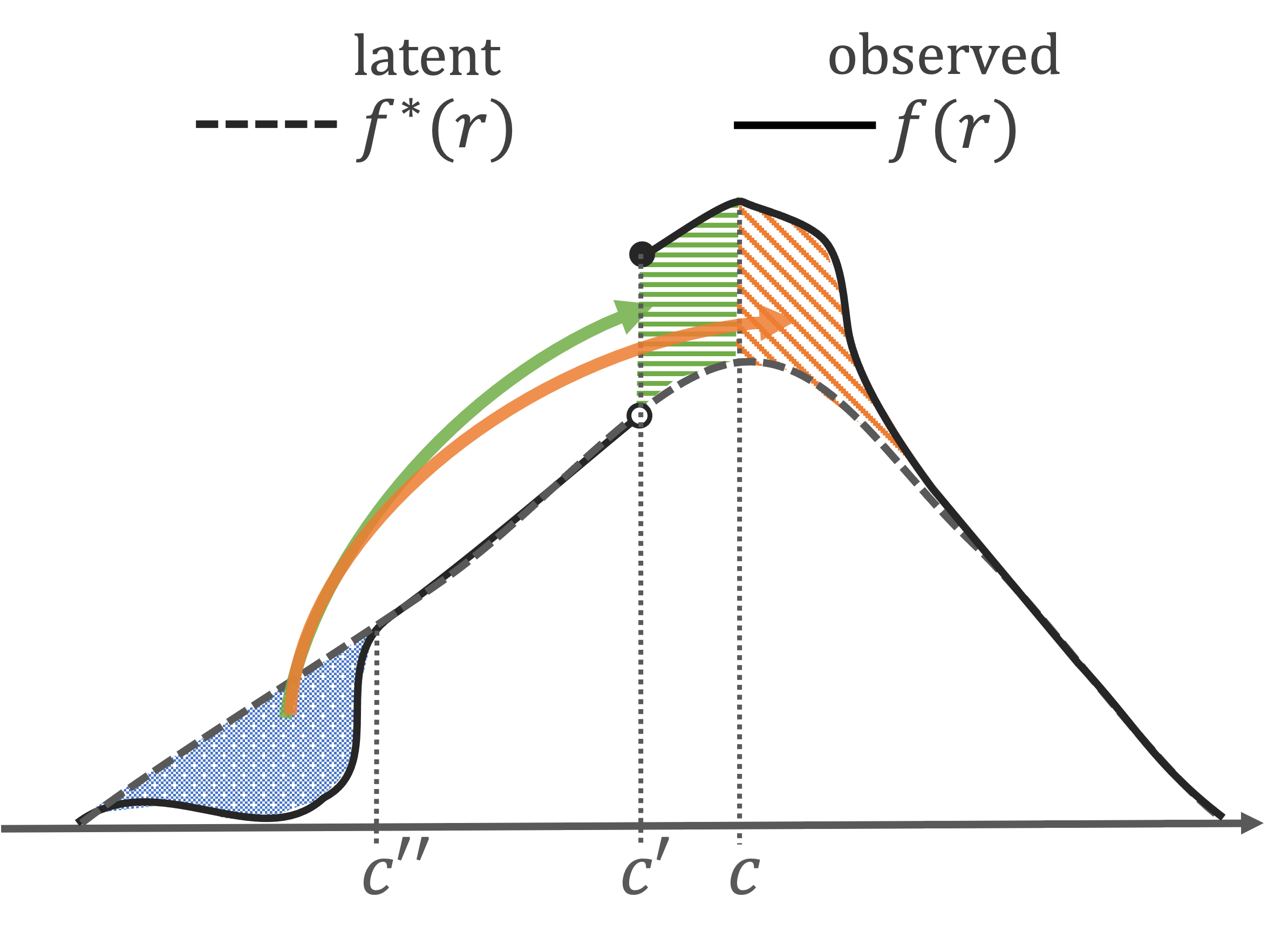
Figure 2.4: Counterexample of monotone manipulation violating detectability.

We provide a counterexample below. Consider teachers offering a retake of the exam. However, now consider that some students intentionally failed to ensure that they would retake the exam. In Figure 2.4, there are two nearby cutoffs, $c$ and $c^{\prime}$. Let the known cutoff $c$ be the official passing cutoff. Let the left cutoff $c^{\prime}$ be a hidden cutoff that is unknown to the researcher but is an internal cutoff for penalizing students below it. Some students who were not ready for the exam and had their $R^{*}$ lower than $c^{\prime\prime}$ (in the blue-dotted region) may have two different manipulation behaviors. Some students may precisely control their $R$ just above the passing cutoff $c$ (in the orange-hatched region) because they believe they will not improve their scores. Other students may want to intentionally fail the exam to retake it because they think they can score higher than just above the cutoff $c$. Nevertheless, these students set $R$ above $c^{\prime}$ (in the green-striped region); otherwise, they would face an additional penalty. These two manipulations are both monotonic but not one-sided because they are sorted just below the policy cutoff $c$. These monotonic manipulations make the density continuous at $c$. However, students’ expected performance in their retaken exam differs from those just above and just below the cutoff $c$; consequently, the identification fails.

Appendix C Other case studies

Example C.1 (Almost clean RD but with a possible precise selection).

Pinotti (2017) studies the effect of receiving a residence permit on an immigrant’s likelihood to commit a crime. A key feature of the design is that “the exact timing of the cutoff for each group was unknown ex-ante, as it depended on the timing of all applications and on how many applications were rejected for being inaccurate, false, or incomplete.” (Pinotti, 2017, p.140). The unknown cutoff remains a compelling argument against precise control as well as precise selection.

Nevertheless, “applicants within an arbitrarily narrow bandwidth of the cutoff were unable to precisely determine their assignment to either side of it” (Pinotti, 2017, p.140) is insufficient for identification. Precise selection remains concerning because “some of the rejected applicants could leave the country (or be expelled) in the months after click days” (Pinotti, 2017, p.149). Fortunately, “obtaining a residence permit in Italy does not allow for free mobility in the rest of the European Union” (Pinotti, 2017, p.149). Attrition from the universe of crime data in Italy is likely to be one-sided: because they are rejected, but not because they are accepted. Hence, the density test is valid.

Example C.2 (Studies with both precise control and selection: Maimonides’ rule redux).

Angrist, Lavy, Leder-Luis, and Shany (2019) is a followup study of Angrist and Lavy (1999). The Maimonides’ rule is the Israeli school system, which determines the number of classrooms by the number of enrolments. In particular, a school with $41$ students must have two classes of $20$ and $21$. The treatment is the assignment to a smaller class.

Angrist et al. (2019) states that “schools are warned not to move students between grades or to enroll those overseas so as to produce an additional class” (page. 310) from the Israeli Ministry of Education (MOE). Such manipulation is a typical complete manipulation that precisely controls the class size in a precisely selected school. These manipulations (moving students between grades or inviting students from overseas) are costly and hence should occur only among schools below the cutoff and only to exceed the cutoff marginally from $40$ to $41$. These manipulations should be one-sided because “School leaders might care to do this because educators and parents prefer smaller classes. MOE rules that set school budgets as an increasing function of the number of classes also reward manipulation.” (Angrist et al., 2019, page. 310). Hence, the test is valid.

For this valid density test, Otsu et al. (2013) and Angrist et al. (2019) report the discontinuity of the density, but Arai et al. (2021a) report their fuzzy RD test passes. These test results are consistent because continuous density is not necessary for identification. As seen in (2.1) and Examples 2.1 and 2.2, identification failure is driven by the difference in the manipulators and non-manipulators. Angrist et al. (2019) verify that the index of socioeconomic status is similar, and their identification can be valid.

Example C.3 (Studies that propose bounds related to $\Gamma_{+}$ and $\Gamma_{-}$).

Card, Dobkin, and Maestas (2009) consider an age-based (at 65) RD for Medicaid eligibility on mortality rates. In their Appendix, they consider Manski-type worst-case bounds in the form of $\Gamma_{+}$ bounds. Local randomization fails when there are some elderly people “who will only enter the hospital if they are over 65” (Card et al., 2009, page. 13). This manipulation is a precise selection. If no one can manipulate their Medicare eligibility by manipulating their birthday, then precise control is not possible. $\Gamma_{+}$ has a straightforward interpretation that is as good as $E[Y(1)-Y(0)|R^{*}=c]$. Mortality is binary, and Lee-bounds do not necessarily improve against Manski-bounds. Hence, $\Gamma_{+}$ bounds are appropriate.

Sallee (2011) also considers the $\Gamma_{+}$ type bounds for the impact of a tax credit for particular hybrid cars in the U.S. on the price of a new Toyota Prius. Sallee (2011) concerns that “A mover with an ideal date of purchase near a tax change will move their transaction into the high subsidy period” (page. 202) buys Prius only after the tax change period. This manipulation is a precise selection. By contrast, this manipulation is also a precise control because the ideal date of purchase $R^{*}$ may have been before the tax change but the mover moves $R$ to $R\geq c$. Hence, neither $\Gamma_{+}$ nor $\Gamma_{-}$ provides a clean interpretation. $\Gamma_{+}$ is the ATE of those who had their ideal date at $R^{*}=c$ plus the movers who moved their purchase date to $R=c_{+}$. $\Gamma_{-}$ is the ATE of $R^{*}=c$ minus that of the movers who moved away from their original purchase date as $R^{*}=c_{-}$. Nevertheless, the Lee-type bounds for $\Gamma_{-}$ may be appropriate for this study because the outcome variable is the price of a car that has no apparent upper bound value.

Anderson and Magruder (2012) consider the effect of getting a better star in the online review platform (Yelp.com) on restaurants’ reservation availability. Anderson and Magruder (2012) concern that the restaurant owners may have manipulated their scores by submitting fake reviews in favor of their restaurants to get a higher rounded score. Anderson and Magruder (2012) claim that the incentive to submit fake reviews is continuous across the threshold because “given that a random stream of reviews will change each restaurant’s average rating over any time period, a restaurant which is just above a threshold has a very similar likelihood of just missing that threshold after new reviews come in as a restaurant which is just below the threshold” (page. 14). Unlike the intent of the authors, such owners’ behavior may violate the one-sided restriction.

Finally, Schmieder, von Wachter, and Bender (2012) consider an RD analysis of UI benefits with their eligibility determined by birthdays. Schmieder et al. (2012) consider $\Gamma_{-}$ bounds. Nevertheless, the leading concern of manipulation is that firms are more likely to lay off older workers who can receive additional UI benefits. As in Card et al. (2009), workers cannot manipulate their age for UI benefit eligibility. As a result, no precise control is possible; however, precise selection is possible. Hence, $\Gamma_{+}$ may provide a better interpretation than $\Gamma_{-}$. Nevertheless, the outcome variable of UI duration is non-binary. Hence, $\Gamma_{-}$ bounds may be preferable, because $\Gamma_{+}$ bounds can be uninformative.

References

- Abdulkadiroğlu et al. (2022) Abdulkadiroğlu, A., J. D. Angrist, Y. Narita, and P. Pathak (2022): “Breaking Ties: Regression Discontinuity Design Meets Market Design,” Econometrica, 90, 117–151.