Approach to equilibrium and non-equilibrium stationary distributions of interacting many-particle systems that are coupled to different heat baths

Abstract

A Hamiltonian-based model of many harmonically interacting massive particles that are subject to linear friction and coupled to heat baths at different temperatures is used to study the dynamic approach to equilibrium and non-equilibrium stationary states. An equilibrium system is here defined as a system whose stationary distribution equals the Boltzmann distribution, the relation of this definition to the conditions of detailed balance and vanishing probability current is discussed both for underdamped as well as for overdamped systems. Based on the exactly calculated dynamic approach to the stationary distribution, the functional that governs this approach, which is called the free entropy ${\cal S}_{\rm free}(t)$, is constructed. For the stationary distribution ${\cal S}_{\rm free}(t)$ becomes maximal and its time derivative, the free entropy production $\dot{\cal S}_{\rm free}(t)$, is minimal and vanishes. Thus, ${\cal S}_{\rm free}(t)$ characterizes equilibrium as well as non-equilibrium stationary distributions by their extremal and stability properties. For an equilibrium system, i.e. if all heat baths have the same temperature, the free entropy equals the negative free energy divided by temperature and thus corresponds to the Massieu function which was previously introduced in an alternative formulation of statistical mechanics. Using a systematic perturbative scheme for calculating velocity and position correlations in the overdamped massless limit, explicit results for few particles are presented: For two particles localization in position and momentum space is demonstrated in the non-equilibrium stationary state, indicative of a tendency to phase separate. For three elastically interacting particles heat flows from a particle coupled to a cold reservoir to a particle coupled to a warm reservoir if the third reservoir is sufficiently hot. This does not constitute a violation of the second law of thermodynamics, but rather demonstrates that a particle in such a non-equilibrium system is not characterized by an effective temperature which equals the temperature of the heat bath it is coupled to. Active particle models can be described in the same general framework, which thereby allows to characterize their entropy production not only in the stationary state but also in the approach to the stationary non-equilibrium state. Finally, the connection to non-equilibrium thermodynamics formulations that include the reservoir entropy production is discussed.

I Introduction

Systems that even in their stationary state are not in equilibrium have in the last decades received renewed attention since standard concepts of thermodynamics and statistical mechanics do not work and because of their experimental relevance Onsager (1931); Prigogine (1947); Prigogine and Mazur (1953); Lebowitz (1959); Graham and Haken (1971); Schlögl (1971); Procaccia and Levine (1976); Schnakenberg (1976); Oono and Paniconi (1998); Hatano and Sasa (2001); Esposito et al. (2007); Ramaswamy (2010); Chou et al. (2011); Seifert (2012). Some of the motivation for studying such systems comes from experimental observations of molecular processes in living systems, which are fundamentally non-equilibrium (NEQ)Marchetti et al. (2013); Gnesotto et al. (2018). Apart from biological applications, experimental advances allow for the construction of NEQ systems either from biological components that are driven out of equilibrium by ATP consumption or by using macromolecular and colloidal assemblies that can be driven out of equilibrium by chemical fuels or by applying external forcesBechinger et al. (2016); Illien et al. (2017).

Two prominent features of NEQ systems are departures from the canonical Boltzmann distribution and violation of the fluctuation-dissipation theorem, which were recently demonstrated to go hand in hand for a harmonically coupled particle system Netz (2018), the fundamental hallmark of NEQ systems is the violation of the detailed balance condition Graham and Haken (1971); Schnakenberg (1976). A particularly striking example for the breakdown of equilibrium statistical mechanics is the occurrence of phase transitions induced by NEQ driving. As a result of external forces acting on particle systems, laning and phase separations have been observed Katz et al. (1983); Krug (1991); Schmittmann and Zia (1998); Dzubiella et al. (2002); Netz (2003); Kumar et al. (2014). Internal NEQ effects can generate particle propulsion that is sustained by chemical or biochemical means. NEQ effects can also be induced by stochastic forces due to the coupling of particles to different heat or chemical energy reservoirs. Such internal NEQ effects have also been shown to lead to clustering and phase separation Bertin et al. (2006); Theurkauff et al. (2012); Golestanian (2012); Speck et al. (2014); Ginot et al. (2015); Grosberg and Joanny (2015); Weber et al. (2016); Tanaka et al. (2017); Smrek and Kremer (2017); Chari et al. (2019). Experimentally, symmetry-breaking transitions in suspensions of swimming bacteria and filament systems driven by motor proteins have indeed been demonstrated Sokolov et al. (2007); Suzuki and Bausch (2017). Also in more coarse-grained models, defined by migration rules, collective ordering can be obtained and describes the response of pedestrians to spatial confinement or the flocking and swarming of animals Helbing (2001); Ramaswamy (2010). NEQ transformations also occur for polymers that are driven by externally applied torques Wolgemuth et al. (2000); Wada and Netz (2009).

The equilibrium fluctuation-dissipation theorem (FDT) describes the dynamical response of an equilibrium system to a small perturbation. Since it is a key concept for systems close to equilibrium, and since any violation of the FDT clearly signals that a system is off equilibrium, the derivation of generalized fluctuation-dissipation relations that also hold for NEQ systems is central and has been discussed in the context of laser Agarwal (1972), chaotic Hohenberg and Shraiman (1989), glassy Cugliandolo et al. (1997), driven colloidal Speck and Seifert (2006), sheared Xu and O’Hern (2005); Ilg and Barrat (2007); Krüger and Fuchs (2009) and active systems Levis and Berthier (2015). Generalized NEQ fluctuation-dissipation relations were derived Agarwal (1972); Harada and Sasa (2005); Zamponi et al. (2005); Prost et al. (2009); Baiesi et al. (2009); Seifert and Speck (2010); Willareth et al. (2017) and compared with experimental data for glasses Jabbari-Farouji et al. (2008), colloids Gomez-Solano et al. (2009); Mehl et al. (2010), bundles of biological filaments Martin et al. (2001); Dinis et al. (2012), living cells Bohec et al. (2013) and biological gels that are driven by motor proteins in the presence of ATPMizuno et al. (2007); Netz (2018).

Significant theoretical progress has been made in the characterization of NEQ systems by generalized NEQ fluctuation-dissipation relations, as discussed above, and by fluctuation relations that give bounds and exact relations involving trajectory ensembles Lebowitz and Spohn (1999); Crooks (1999); Jarzynski (2000). The field of stochastic thermodynamics has linked the statistics of trajectories to entropy-production contributions Seifert (2005, 2012). A good fraction of contemporary work on NEQ systems is concerned with analyzing the solutions of governing dynamic equations either by simulation techniques or, for simple systems, by analytical methods. In essence, and as acknowledged by most workers in the field, NEQ theory is far from the predictive power and understanding furnished by e.g. the usage of thermodynamic potentials in the context of equilibrium scenarios. For an isolated system the entropy is maximized, but this provides little help for the type of NEQ problems one is typically interested in, because they are not isolated. For a system coupled to a single heat reservoir and in the absence of external driving forces, which gives rise to the equilibrium canonical ensemble, the free energy is minimized. The free energy, when evaluated exactly or approximately, allows to predict phase transitions, structures and all static properties of an equilibrium system. In the search for a similarly useful framework, the first theoretical studies on NEQ systems formulated general extremal principles that express the system’s tendency to extremize its dissipation, i.e., its entropy production Prigogine (1947); Prigogine and Mazur (1953). These early extremal principles were limited to linear and homogeneous systems close to equilibrium and included interactions only indirectly in terms of phenomenological coefficients. Subsequently, the Master equation approach allowed to derive extremal principles for general NEQ stationary states in terms of a generalized entropy Graham and Haken (1971); Schlögl (1971); Schnakenberg (1976); Esposito et al. (2007). More recently, Onsager’s variational principleOnsager (1931) was revisited and used for the study of various NEQ problems in soft condensed matter Doi et al. (2019).

In this paper we start from a quadratic Hamiltonian model with general interactions. By adding friction terms and stochastic fields to the Hamilton equations, we arrive at the general linear Hamiltonian-based many-dimensional Langevin equation that, for suitably chosen friction and stochastic parameters, describes a many-body system of massive particles coupled to multiple heat baths with different and well-defined temperatures, a model that corresponds to the non-equilibrium version of the multidimensional Ornstein-Uhlenbeck process and has in certain limits been studied in literature Lebowitz (1959); Rieder et al. (1967); Zwanzig (1973); Filliger and Reimann (2007); Prost et al. (2009); Dadhichi et al. (2018); Li et al. (2019). The explicit presence of heat baths with different temperatures allows us to prepare the system in a unique NEQ stationary state and to calculate all contributions to the entropy production as the system approaches the stationary state. Instead of considering trajectories in phase space, we base our theory on the time-dependent distribution. The key point of our model is that we can exactly calculate the time derivative of the distribution entropy and from that construct, by comparison with the independently calculated relaxation of the distribution, the time-dependent functional that governs the approach to equilibrium as well to NEQ stationary distributions. In analogy to the relation between the energy and the free energy, this functional is called the free entropy, ${\cal S}_{\rm free}(t)$, since it contains the distribution entropy of the system and also accounts for the interactions within the system and the coupling to the reservoirs. Using the free entropy ${\cal S}_{\rm free}(t)$, the total entropy ${\cal S}_{\rm tot}(t)$, wich includes the entropy of the interacting particle system ${\cal S}(t)$ as well as the reservoir entropy ${\cal S}_{\rm res}(t)$, can be decomposed as

$${\cal S}_{\rm tot}(t)={\cal S}(t)+{\cal S}_{\rm res}(t)={\cal S}_{\rm free}(t)+t\dot{\cal S}^{\circ}_{\rm res}$$ (1)

up to unimportant constants, where $\dot{\cal S}^{\circ}_{\rm res}$ denotes the entropy production due to heat transfer with all reservoirs in the unique stationary state. While ${\cal S}_{\rm res}(t)$ is difficult to calculate for the stochastic models used for the description of heat reservoirs and in fact increases boundlessly, ${\cal S}_{\rm free}(t)$ and $\dot{\cal S}^{\circ}_{\rm res}$ can be explicitly calculated. Similar to the free energy of statistical mechanics, different observables can be derived from the free entropy by taking suitable derivatives, as is shown in Sect. IV.1.

For an equilibrium system, i.e. when all heat baths have the same temperature and $\dot{\cal S}^{\circ}_{\rm res}=0$, and in the stationary state, the free entropy is time-independent and equals the negative free energy divided by temperature, i.e.

$${\cal S}^{\bullet}_{\rm free}=-{\cal F}^{\bullet}/T={\cal S}^{\bullet}-{\cal U}^{\bullet}/T,$$ (2)

where filled circles in our paper denote the equilibrium stationary state. In fact, the free entropy functional had been used by Massieu already in 1869 Callen (1985); Balian (2017), a few years before Gibbs introduced his energy transforms. The advantage of the free entropy functional has been pointed out by Planck Planck (1945) and Schrödinger Schrödinger (1964), while the name was introduced more recently in the mathematical literature Biane and Speicher (2001); Voiculescu (2002). The free entropy is central in the context of our model, since the presence of different heat bath temperatures does not allow to define a unique NEQ version of the free energy. In a number of previous papers functionals were derived that in a NEQ stationary state are extremal and thereby allow to study the relaxation and the stability of NEQ systems and the relation of these functionals to the Kullback-Leibler entropyKullback and Leibler (1951) was pointed out Graham and Haken (1971); Schlögl (1971); Procaccia and Levine (1976); Schnakenberg (1976); Kwon et al. (2005); Esposito et al. (2007); Ge (2009); Ge and Qian (2010); Qian (2013, 2015). Our model differs from those works since we introduce NEQ by the coupling to multiple heat baths with different temperatures. While the early approaches to NEQ thermodynamics were centered on the total entropy production $\dot{\cal S}_{\rm tot}(t)$, i.e. the time derivative of the total entropy including the reservoirs Prigogine (1947); Prigogine and Mazur (1953), in later developments the entropy production due to heat transfer from the reservoirs, which in a NEQ stationary state is constant and given by $\dot{\cal S}^{\circ}_{\rm res}$, has been separated off and called the house-keeping entropy Oono and Paniconi (1998); Hatano and Sasa (2001); Speck and Seifert (2005). One advantage of our model is that since the particles have finite masses, the heat fluxes between the particles and the heat reservoirs can be calculated from energy balance considerations including the kinetic energy and thus the stationary reservoir entropy production $\dot{\cal S}^{\circ}_{\rm res}$ can be derived straightforwardly. For this we introduce a systematic perturbation scheme using the particle masses as expansion parameters to calculate NEQ mixed position-velocity correlations.

We here show that for a system coupled to different temperature reservoirs, the free entropy functional ${\cal S}_{\rm free}(t)$ can be written down explicitly and is for the NEQ stationary distribution maximal and constant in time. The free entropy production $\dot{\cal S}_{\rm free}(t)$ is positive except at the stationary NEQ state, for which it vanishes, i.e.

$$\dot{\cal S}_{\rm free}(t)\geq 0.$$ (3)

This shows that the NEQ stationary state is stable with respect to small perturbations and that in the NEQ stationary state the total entropy production is given solely by the reservoirs. The time derivative of the free entropy production, which would be the second time derivative of the free entropy, is not needed, unlike early NEQ approaches Prigogine (1947); Prigogine and Mazur (1953). Our framework thus treats NEQ and equilibrium systems on the same footing, as for an equilibrium system the NEQ free entropy smoothly crosses over to the standard free energy divided by $-T$, see Eq. (2), and so the standard equilibrium and stability conditions of statistical mechanics are recovered.

Interestingly, the dynamic approach to the equilibrium and to the NEQ stationary distributions obey the same differential equation, as is shown in Sect. III.3. In fact, while equilibrium and NEQ stationary distributions exhibit many fundamental differences, the relaxation times that characterize the approach to stationarity are independent of the heat bath temperatures and therefore do not allow to distinguish equilibrium from NEQ systems. While this might be a simplification due to our neglect of non-linear interactions, we argue that non-linear systems can typically be quadratically approximated around locally stable states and thus our results should also apply to sufficiently well-behaved non-linear systems.

We also demonstrate that the definition of equilibrium we are using in this paper, which is based on the Boltzmann distribution, is equivalent to the detailed-balance condition only if the friction matrix is symmetric and if the random fields couple separately to position and velocity degrees of freedom. For a simple system consisting of two coupled massive particles, we show that if the Boltzmann distribution is realized, the fluctuation-dissipation theorem is satisfied, even when the friction matrix is asymmetric (and thus the condition of detailed balance is not satisfied). This shows that equilibrium definitions based on Boltzmann statistics, on the fluctuation-dissipation theorem and on the detailed-balance condition are equivalent only for symmetric friction matrices and that the detailed-balance condition is the strictest of all three.

As a simple application of our model we present results for three interacting massive particles that are coupled to temperature reservoirs at different temperatures, for which we demonstrate that heat flows from a particle coupled to a cold reservoir to a particle coupled to a warm reservoir if the third reservoir is sufficiently hot. This of course does not constitute a violation of the second law of thermodynamics. Rather, this NEQ entrainment effect can be rationalized by the fact that the reservoirs are not coupled directly to each other but rather indirectly via the particles, and that the particles are not characterized solely by the heat bath temperatures. This point can be explained in more detail by considering just two particles that are coupled to different heat baths: We demonstrate that the concept of a NEQ effective temperature has only a rather limited value, since each covariance matrix entry of two coupled NEQ particles would have to be attributed a different effective temperature. For two particles we also demonstrate that NEQ effects give rise to localization effects both in position and in momentum space, which is reminiscent of attractive interactions. This reflects the tendency of NEQ systems to phase separate in both position and momentum space. Finally, we show how active particle models can be described using our general framework and discuss the connection between the free entropy production and the total entropy production that includes the reservoirs.

In the following sections we first treat general NEQ systems and derive the necessary conditions to reach a stationary state and a stationary equilibrium state, described by the Lyapunov and the Lyapunov-Boltzmann equations, respectively. In Sect. IV.2 we start treating the core model of this paper, where particles are coupled to heat reservoirs that are characterized by different temperatures, and present various explicit examples.

II Many-Particle Hamiltonian Model

II.1 From Hamilton to Langevin equations

To proceed, we consider $N$ massive particles in one dimension with positions $x_{\alpha}$ and momenta $p_{\alpha}$ that move according to the Hamilton equations

$$\dot{x}_{\alpha}(t)=\frac{\partial{\cal H}(\vec{x},\vec{p})}{\partial p_{\alpha}},$$ (4)

$$\dot{p}_{\alpha}(t)=-\frac{\partial{\cal H}(\vec{x},\vec{p})}{\partial x_{\alpha}},$$ (5)

where $\alpha=1\ldots N$ is an index that runs over all particles. The case of $M$ interacting particles in three dimensions is described by $N=3M$ particle coordinates and is implicitly included in our model. Using the antisymmetric matrix

$$U=\begin{pmatrix}0&1&0&0&\\ -1&0&0&0&\\ 0&0&0&1&\\ 0&0&-1&0&\\ &&&&\ddots\end{pmatrix}$$ (6)

and the state vector

$$\vec{z}(t)=(x_{1}(t),p_{1}(t),x_{2}(t),p_{2}(t)\ldots)^{T}$$ (7)

the Hamilton equations can be written compactly as

$$\dot{z}_{i}(t)=U_{ij}\frac{\partial{\cal H}(\vec{z})}{\partial z_{j}},$$ (8)

where $i=1\ldots 2N$ is an index that runs over all position and momentum coordinates. Throughout this paper, greek indices denote particles (running from 1 to $N$), roman indices denote coordinates (running from 1 to $2N$) and indices that appear more than once are summed over except primed indices. We consider quadratic Hamiltonians of the form

$${\cal H}(\vec{z})=z_{i}H_{ij}z_{j}/2$$ (9)

that are described by a general symmetric matrix $H$ which we assume to be positive definite, i.e., ${\cal H}(\vec{z})>0$ for general $\vec{z}$. A possible linear term in the Hamiltonian can be absorbed into the definition of the state vector $z_{j}$ and need not be considered explicitly. For quadratic Hamiltonians the Hamilton equations are linear and given by

$$\dot{z}_{i}(t)=U_{ij}H_{jk}z_{k}(t).$$ (10)

More specific forms of the Hamiltonian matrix $H$, in particular Newtonian Hamiltonians where momentum und position degrees of freedom are decoupled, will be discussed later, in the first part of this paper the discussion applies to general Hamiltonian models.

By adding linear friction terms and random fields to the Hamilton equations, which will be later shown to mimic the coupling to heat baths with in general different temperatures, we obtain the coupled linear Langevin equations

$$\dot{z}_{i}(t)=U_{ij}H_{jk}z_{k}(t)-\Gamma_{ik}z_{k}(t)+\Phi_{ik}F_{k}(t)$$ (11)

which by definition of the generally asymmetric coupling matrix

$$A_{ik}=-U_{ij}H_{jk}+\Gamma_{ik}$$ (12)

can be written more compactly as

$$\dot{z}_{i}(t)=-A_{ik}z_{k}(t)+\Phi_{ik}F_{k}(t).$$ (13)

Here, $\Gamma$ is the friction coefficient matrix and $\Phi$ is the random strength matrix that describes how random fields couple to different particle coordinates. For simplicity, we assume Gaussian white random fields with zero mean $\langle F_{i}(t)\rangle=0$ and and variances $\langle F_{i}(t)F_{j}(t^{\prime})\rangle=2\delta_{ij}\delta(t-t^{\prime})$. Non-Markovian models with colored noise can be obtained by integrating out degrees of freedom and need not explicitly be considered Zwanzig (1961). In standard friction models friction forces couple to the momentum degree of freedom and are proportional to particle velocities. In more elaborate models that include hydrodynamic interactions, the friction force acting on a given particle depends on the velocities of all particles. In the first part of this paper the matrices $\Gamma$ and $\Phi$ are kept general and $\Gamma$ can also be asymmetric (which will be shown to have direct consequences for the detailed-balance condition in Sect. III.4). In the second part of the paper, starting in Sect. IV.2, we model heat baths with different temperatures and for this will assume $\Gamma$ and $\Phi$ to be diagonal. The general form of the linear Langevin Eq. (13) does not directly reveal whether it describes an equilibrium or a NEQ systemDadhichi et al. (2018), this point will be addressed further below.

II.2 Stationary distribution

The algebraic solution of the Langevin Eq. (13) is

$$z_{i}(t)={\rm e}^{-tA}_{ij}z_{j}(0)+\int_{0}^{t}{\rm d}t^{\prime}{\rm e}^{-(t-t^{\prime})A}_{ij}\Phi_{jk}F_{k}(t^{\prime}),$$ (14)

where $z_{j}(0)$ denotes the initial particle positions and momenta at time zero. The average over the noise gives

$$\langle z_{i}(t)\rangle={\rm e}^{-tA}_{ij}z_{j}(0)$$ (15)

which can be viewed as the solution of the noise-averaged version of the Langevin Eq. (13)

$$\langle\dot{z}_{i}(t)\rangle=-A_{ik}\langle z_{k}(t)\rangle.$$ (16)

If all eigenvalues of the matrix $A$ have positive real components, a unique stationary distribution exists and is characterized by a vanishing mean $\langle z_{i}(t\rightarrow\infty)\rangle=0$.

The covariance matrix of the deviations from the mean $\Delta z_{i}(t)=z_{i}(t)-\langle z_{i}(t)\rangle$ follows from squaring the solution Eq. (14) and averaging over the noise, leading toRisken (1984)

$$E_{ij}(t)\equiv\langle\Delta z_{i}(t)\Delta z_{j}(t)\rangle=2\int_{0}^{t}{\rm d}t^{\prime}{\rm e}^{-(t-t^{\prime})A}_{ik}{\rm e}^{-(t-t^{\prime})A}_{jl}C_{kl},$$ (17)

where the random correlation matrix is defined by

$$C_{kl}=\Phi_{km}\Phi_{lm}=C_{lk}$$ (18)

and is symmetric by construction. Since

$$A_{ik}E_{kj}+A_{jk}E_{ki}=A_{ik}E_{kj}+A_{jk}E_{ik}=$$

$$2\int_{0}^{t}{\rm d}t^{\prime}\frac{\rm d}{{\rm d}t^{\prime}}{\rm e}^{-(t-t^{\prime})A}_{ik}{\rm e}^{-(t-t^{\prime})A}_{jl}C_{kl},$$ (19)

the stationary covariance matrix, denoted by an open circle and defined by

$$E^{\circ}_{ij}\equiv E_{ij}(t\rightarrow\infty),$$ (20)

is unique and given by the Lyapunov equation

$$2C_{ij}=A_{ik}E_{kj}^{\rm\circ}+A_{jk}E_{ki}^{\rm\circ}$$ (21)

if all eigenvalues of the matrix $A$ have positive real parts, which we will assume to be true throughout this paper.

III Systems that have an equilibrium distribution

III.1 Distributions, entropy and free energy

In equilibrium, the normalized distribution in terms of the state vector $\vec{z}$ is given by the Boltzmann distribution

$$\rho(\vec{z})={\rm e}^{-\beta{\cal H}(\vec{z})}/{\cal Z},$$ (22)

where $\beta=1/(k_{B}T)$ denotes the inverse thermal energy and ${\cal Z}=\int{\rm d}\vec{z}{\rm e}^{-\beta{\cal H}(\vec{z})}$ is the partition function. We will discuss the connection of this definition of equilibrium to the conditions of detailed balance, vanishing probability current as well as  the fluctuation-dissipation theorem in Sect. III.4. Positive definiteness of the Hamiltonian matrix $H$ guarantees that ${\cal Z}$ is finite (if the Hamiltonian is invariant with respect to one or few degrees of freedom they can be separated off to make the reduced Hamiltonian positive definite). For a quadratic Hamiltonian, the average state vector vanishes and all covariances can be calculated from the Boltzmann distribution, which only involves inversion of the Hamiltonian matrix.

For the later discussion of the NEQ scenario, it is instructive to derive the equilibrium distribution also via the thermodynamic route. From the thermodynamic definitions of the free energy ${\cal F}=-k_{B}T\ln{\cal Z}$ and the entropy ${\cal S}=-\partial{\cal F}/\partial T$, the Shannon expression for the entropy directly follows as

$${\cal S}/k_{B}=-\int{\rm d}\vec{z}\rho(\vec{z})\ln\rho(\vec{z}),$$ (23)

the derivation is shown in Appendix A. Note that the Shannon expression Eq. (23) can also be used to describe the distribution entropy for time-dependent distributions, i.e. for non-stationary and even NEQ situations, since the expression makes no reference to the equilibrium ensemble or to the presence of a heat bath. This will allow us to describe the time-dependent approach to equilibrium as well as to stationary NEQ distributions.

For the linear Langevin Eq. (13), the time-dependent probability distribution is Gaussian and can be written as

$$\rho(\vec{z},t)=\hskip 142.26378pt$$ (24)

$${\cal N}^{-1}(t)\exp\left(-[z_{i}-\langle z_{i}(t)\rangle]E^{-1}_{ij}(t)[z_{j}-\langle z_{j}(t)\rangle]/2\right),$$

where the time-dependent normalization constant is given by

$${\cal N}(t)=\sqrt{(2\pi)^{2N}\det E(t)}$$ (25)

and only exists if the covariance matrix $E(t)$ is positive definite (note that by its definition $E(t)$ is also symmetric). The proof is standard textbook material Risken (1984), in Appendix B we present a derivation based on random-field path integrals, which has the advantage that it can in principle be generalized to non-Gaussian colored noise; there we furthermore demonstrate that the expression Eq. (24) is in fact the Green’s function of the general Langevin Eq. (13), i.e., the conditional probability distribution at time $t$ for the case that the distribution is a delta function at time $t=0$.

With the Gaussian form Eq. (24), the integral in Eq. (23) can be performed and yields the time-dependent distribution entropy as

$${\cal S}(t)/k_{B}=N+\ln{\cal N}(t)=N+(1/2)\ln[(2\pi)^{2N}\det E(t)].$$ (26)

The internal energy is given by

$${\cal U}(t) =\langle{\cal H}(\vec{z}(t))\rangle=H_{ij}\langle z_{i}(t)z_{j}(t)\rangle/2$$

$$=H_{ij}\langle z_{i}(t)\rangle\langle z_{j}(t)\rangle/2+H_{ij}E_{ij}(t)/2.$$

With these results for the entropy and internal energy, the free energy

$${\cal F}(t)={\cal U}(t)-T{\cal S}(t)$$ (28)

follows as

$${\cal F}(t)= H_{ij}\langle z_{i}(t)\rangle\langle z_{j}(t)\rangle/2+H_{ij}E_{ij}(t)/2$$

$$-k_{B}TN-(k_{B}T/2)\ln[(2\pi)^{2N}\det E(t)].$$

The extremum of the free energy is determined by $\langle\vec{z}(t)\rangle=0$ and by

$$\frac{\partial{\cal F}(t)}{\partial E_{ij}}=H_{ij}/2-k_{B}TE^{-1}_{ji}(t)/2=0,$$ (30)

the solution of which is time-independent and defines the equilibrium distribution (denoted by a filled circle) as

$$E_{ij}^{\bullet}=k_{B}TH^{-1}_{ij}.$$ (31)

In deriving Eq. (30) we used the basic algebraic relation $\partial\ln\det E/\partial E_{ij}=E^{-1}_{ji}$. The partial derivative denotes the derivative with respect to one matrix component while keeping all other components fixed. The equilibrium free energy follows by reinserting $\langle\vec{z}(t)\rangle=0$ and the solution $E_{ij}^{\bullet}$ into the free energy expression Eq. (III.1) and is given by

$${\cal F}^{\bullet}=-(k_{B}T/2)\ln[(2\pi k_{B}T)^{2N}/\det H].$$ (32)

We next want to show that the extremum of the free energy is in fact a minimum (for this we neglect the trivial quadratic dependence of Eq. (III.1) on the mean state vector $\langle\vec{z}(t)\rangle$). We first realize that

$$\frac{\partial^{2}{\cal F}(t)}{\partial E_{kl}\partial E_{ij}}=k_{B}TE^{-1}_{ik}(t)E^{-1}_{lj}(t)/2,$$ (33)

where we used the basic algebraic relation $\partial E^{-1}_{kn}/\partial E_{ij}=-E^{-1}_{ki}E^{-1}_{jn}$. Around the equilibrium distribution $E_{ij}=E^{\bullet}_{ij}$ the free energy is to second order given by

$${\cal F}(t)-{\cal F}^{\bullet}\simeq$$ (34)

$$H_{ki}(E_{ij}(t)-H^{-1}_{ij}k_{B}T)H_{jl}(E_{lk}(t)-H^{-1}_{lk}k_{B}T)/(2k_{B}T),$$

which can be rewritten as

$${\cal F}(t)-{\cal F}^{\bullet}\simeq\frac{k_{B}T(\delta_{il}-\beta H_{ik}E_{kl}(t))(\delta_{il}-\beta H_{lk}E_{ki})}{2}.$$ (35)

The latter form is quadratic and of the general form ${\cal F}(t)-{\cal F}^{\bullet}\simeq k_{B}TB_{il}B_{li}/2$ with $B_{il}\equiv\delta_{il}-\beta H_{ik}E_{kl}(t)$, but this by itself does not guarantee that ${\cal F}(t)-{\cal F}^{\bullet}$ is positive since $B_{il}$ is not necessarily symmetric. In Appendix C we show by diagonalization that the positivity of the expression Eq. (34) for ${\cal F}(t)-{\cal F}^{\bullet}$ follows from the fact that $H$ is symmetric and positive definite.

The Gaussian distribution Eq. (24) in conjunction with Eq. (31) is equivalent to the Boltzmann distribution Eq. (22), which we have thus rederived by minimizing the time-dependent free-energy functional Eq. (III.1). But the free energy functional Eq. (III.1) is not only valid in equilibrium but also describes systems that approach the equilibrium distribution. This is an important insight, as this functional framework will allow us to characterize the approach not only to equilibrium but also to stationary NEQ distributions.

III.2 When does a Langevin equation describe an equilibrium system?

In this section we will explore under which conditions the Langevin Eq. (13) describes an equilibrium system, which will put stringent conditions on the random correlation matrix $C$ and on the friction matrix $\Gamma$. We in this paper define a system to be in equilibrium if the stationary state corresponds to the Boltzmann distribution, the relation to other definitions of equilibrium will be discussed in Sect. III.4. We implement this condition by replacing the stationary covariance matrix $E_{ij}^{\circ}$ in the Lyapunov Eq. (21) by the equilibrium covariance matrix $E_{ij}^{\bullet}$ from Eq. (31), by which we obtain

$$2C^{\bullet}_{ij}/(k_{B}T)=A_{ik}H_{kj}^{-1}+A_{jk}H_{ki}^{-1}.$$ (36)

Inserting the expression for the Langevin matrix $A$ from Eq. (12) and using the fact that the matrix $U$ is antisymmetric, see Eq. (6), we arrive at the Lyapunov-Boltzmann equation

$$2C^{\bullet}_{ij}/(k_{B}T)=\Gamma_{ik}H_{kj}^{-1}+\Gamma_{jk}H_{ki}^{-1}.$$ (37)

If for arbitrary Hamiltonian matrix $H$ the friction matrix $\Gamma$ and the random force correlation matrix $C$ obey this equation, the Langevin equation given by Eq. (13) describes the dynamics of an equilibrium system. Conversely, if $C$ and $\Gamma$ do not satisfy Eq. (37) the Langevin equation describes a NEQ system. Two obvious NEQ scenarios come to mind: i) A Newtonian Hamiltonian many-body system coupled to heat baths characterized by different temperatures (as will be discussed starting in Section IV.2), and ii) a many-body system with off-diagonal friction terms that do not obey Eq. (37).

Let us give a simple example, namely the harmonic oscillator with Hamiltonian ${\cal H}=Kx^{2}/2+p^{2}/(2m)$, which is described by the Hamiltonian matrix

$$H=\begin{pmatrix}K&0\\ 0&1/m\\ \end{pmatrix}.$$ (38)

We choose a diagonal momentum friction model described by the friction matrix

$$\Gamma=\begin{pmatrix}0&0\\ 0&\gamma/m\\ \end{pmatrix},$$ (39)

where the friction force is proportional to the velocity of the particle and only enters the momentum degree of freedom. The matrix product appearing on the right side of the Lyapunov-Boltzmann Eq. (37) is given by

$$\Gamma H^{-1}=\begin{pmatrix}0&0\\ 0&\gamma\\ \end{pmatrix}$$ (40)

and thus the equilibrium random correlation matrix follows as

$$C^{\bullet}=\begin{pmatrix}0&0\\ 0&k_{B}T\gamma\\ \end{pmatrix}.$$ (41)

This agrees with the well-known result that the equilibrium Langevin equation of a massive particle involves a random field that acts on the momentum degree of freedom only and is proportional to the friction coefficient $\gamma$, where the proportionality constant $k_{B}T$ defines the temperature of the reservoir. Conversely, any non-trivial deviation of the matrix $C$ from Eq. (41), i.e. any deviation that cannot be captured by a modified temperature, indicates a NEQ system. For the simple example of a one-dimensional harmonic oscillator considered here, this could for example be the presence of an additional entry in the symmetric matrix $C$, e.g. additional entries in the off-diagonals or in the upper-left diagonal.

III.3 Dynamic approach to the stationary distribution

From the time-dependent analogue of the Shannon entropy Eq. (23)

$${\cal S}(t)/k_{B}=-\int{\rm d}\vec{z}\rho(\vec{z},t)\ln\rho(\vec{z},t),$$ (42)

we obtain by differentiation

$$\dot{\cal S}(t)/k_{B}=-\int{\rm d}\vec{z}\dot{\rho}(\vec{z},t)[\ln\rho(\vec{z},t)+1].$$ (43)

The time derivative of the density distribution $\dot{\rho}(\vec{z},t)$ is determined by the Fokker-Planck equation

$$\dot{\rho}(\vec{z},t)=\left[\nabla_{k}A_{km}z_{m}+\nabla_{k}\nabla_{m}C_{km}\right]\rho(\vec{z},t)$$ (44)

which follows via Kramers-Moyal expansion of the Langevin Eq. (13) Risken (1984). With the Gaussian time dependent distribution Eq. (24) we obtain from Eq. (44) the expression

$$\dot{\rho}(\vec{z},t)=\rho(\vec{z},t)\times\hskip 28.45274pt$$ (45)

$$\left[A_{kk}-A_{km}z_{m}E^{-1}_{kj}\Delta z_{j}+C_{ij}(E^{-1}_{ik}\Delta z_{k}E^{-1}_{jl}\Delta z_{l}-E^{-1}_{ij})\right].$$

Inserting this into the expression Eq.(43) and calculating all Gaussian expectation values, we obtain the final expression for the time derivative of the entropy as

$$\dot{\cal S}(t)/k_{B}=C_{km}E^{-1}_{km}(t)-A_{kk},$$ (46)

which holds for equilibrium as well as for NEQ systems. From the Lyapunov Eq. (21) we can derive the expression

$$C_{ij}E^{\circ-1}_{ij}=A_{kk},$$ (47)

inserting this into Eq. (46) we obtain the alternative expression

$$\dot{\cal S}(t)/k_{B}=C_{km}[E^{-1}_{km}(t)-E^{\circ-1}_{km}],$$ (48)

which demonstrates that the entropy change vanishes in the stationary state $E_{km}(t)=E^{\circ}_{km}$, as is expected. We will later come back to Eq. (48) as it allows to write down one of the constitutive dynamic equations for NEQ systems.

We next calculate the time derivative of the covariance matrix. From the expression Eq. (45) we immediately read off that

$$\partial\ln{\rho}(\vec{z},t)/\partial t=\hskip 28.45274pt$$ (49)

$$A_{kk}-A_{km}z_{m}E^{-1}_{kj}\Delta z_{j}+C_{ij}(E^{-1}_{ik}\Delta z_{k}E^{-1}_{jl}\Delta z_{l}-E^{-1}_{ij}),$$

which can be rewritten as

$$\partial\ln{\rho}(\vec{z},t)/\partial t=\Delta z_{i}\Delta z_{j}[C_{km}E^{-1}_{kj}E^{-1}_{mi}-A_{ki}E^{-1}_{kj}]\hskip 8.5359pt$$ (50)

$$+A_{kk}-C_{km}E^{-1}_{km}-A_{km}\langle z_{m}(t)\rangle E^{-1}_{kj}\Delta z_{j}.$$

On the other hand, using the definition of the Gaussian distribution Eq.(24) we find

$$\frac{\partial\ln{\rho}(\vec{z},t)}{\partial t}=\frac{\partial}{\partial t}\left\{-\frac{1}{2}\ln[(2\pi)^{2N}\det E(t)]\right.$$ (51)

$$\left.-\frac{1}{2}[z_{i}-\langle z_{i}(t)\rangle]E^{-1}_{ij}(t)[z_{j}-\langle z_{j}(t)\rangle]\right\},$$

which can be rewritten as

$$\frac{\partial\ln{\rho}(\vec{z},t)}{\partial t}=\langle\dot{z}_{i}(t)\rangle E^{-1}_{ij}(t)\Delta z_{j}\hskip 28.45274pt$$ (52)

$$+\frac{\dot{E}^{-1}_{kl}\partial}{\partial E^{-1}_{kl}}\left\{\frac{1}{2}\ln[(2\pi)^{-2N}\det E^{-1}(t)]-\frac{1}{2}\Delta z_{i}E^{-1}_{ij}(t)\Delta z_{j}\right\}$$

and finally yields

$$\frac{\partial\ln{\rho}(\vec{z},t)}{\partial t}=\langle\dot{z}_{i}(t)\rangle E^{-1}_{ij}\Delta z_{j}+\frac{\dot{E}^{-1}_{kl}}{2}\left\{E_{kl}(t)-\Delta z_{k}\Delta z_{l}\right\}.$$ (53)

Comparison of Eqs. (50) and (53) term by term yields

$$\dot{E}^{-1}_{ij}(t)=-2C_{km}E^{-1}_{kj}(t)E^{-1}_{mi}(t)+E^{-1}_{jk}(t)A_{ki}+E^{-1}_{ik}(t)A_{kj},$$ (54)

where we have used Eq. (16). From the basic algebraic relation $\dot{E}_{il}(t)=-E_{ij}(t)\dot{E}^{-1}_{jk}(t)E^{-1}_{kl}(t)$ we finally obtain from Eq.(54) the temporal change of the covariance matrix as

$$\dot{E}_{ij}(t)=2C_{ij}-A_{ik}E_{kj}(t)-A_{jk}E_{ki}(t)$$ (55)

which, using Eq.(21), can be rewritten as

$$\dot{E}_{ij}(t)=-A_{ik}[E_{kj}(t)-E^{\circ}_{kj}]-A_{jk}[E_{ki}(t)-E^{\circ}_{ki}].$$ (56)

Note that this expression holds for equilibrium as well as for NEQ systems. As would be expected, the temporal change of the covariance matrix vanishes in the stationary state, i.e. when $E_{km}(t)=E^{\circ}_{km}$.

III.4 Conditions of detailed balance and vanishing probability current

Our definition of equilibrium employs the Boltzmann distribution Eq. (22) and not the condition of detailed balance, which is often used as the defining property of equilibrium de Groot and Mazur (1962). The reason for using the Boltzmann condition is that it is very easy to implement, while the condition of detailed balance is for underdamped many-particle systems rather involved. In fact, for overdamped systems the detailed balance condition becomes equivalent to the condition of vanishing probability current Graham and Haken (1971); Schnakenberg (1976), which in literature is also called the potential condition. We will in this section formulate the condition for the probability current to vanish and then compare with the detailed balance condition, for which the derivation is presented in Appendix D.

The Fokker-Planck Eq. (44) can be interpreted as a balance equation

$$\dot{\rho}(\vec{z},t)=-\nabla_{k}{\cal J}_{k}(\vec{z},t)$$ (57)

with the probability current ${\cal J}(\vec{z},t)$ being given as

$${\cal J}_{k}(\vec{z},t)=-\left[A_{km}z_{m}+\nabla_{m}C_{km}\right]\rho(\vec{z},t).$$ (58)

For the Gaussian distribution Eq. (24) we obtain (for simplicity we set $\langle z_{i}(t)\rangle=0$ here) for the current

$${\cal J}_{k}(\vec{z},t)=-\left[A_{km}-C_{kj}E_{mj}^{-1}\right]z_{m}\rho(\vec{z},t).$$ (59)

The probability current vanishes, i.e. ${\cal J}_{k}(\vec{z},t)=0$, for

$$A_{km}E_{mj}=C_{kj}.$$ (60)

From the equilibrium condition $E_{kj}(t)=E^{\bullet}_{kj}=k_{B}TH^{-1}_{kj}$, Eq. (31), and the explicit form of the matrix $A$ in Eq. (12), we obtain the vanishing probability current condition

$$\Gamma_{km}H^{-1}_{mj}-U_{kj}=C_{kj}/(k_{B}T),$$ (61)

which in the general case is not satisfied in the equilibrium situation defined by the Lyapunov-Boltzmann Eq. (37), since $C$ is a symmetric matrix, while $U$ is antisymmetric and typically $\Gamma_{km}H^{-1}_{mj}$ is an asymmetric matrix. We conclude that for an underdamped system, the probability generally does not vanish, this is trivially illustrated by the fact that a harmonic oscillator performs orbits in phase space. In fact, current mathematical work is devoted to separating phase space trajectories of underdamped systems into periodic and diffusive parts Qian (2013, 2015). In Appendix E we show that in the overdamped (i.e. massless) limit the probability current in equilibrium vanishes if the friction matrix $\Gamma$ is symmetric. Since we did not impose that $\Gamma$ is symmetric so far, we see that our definition of equilibrium, which is based on the stationary distribution being equal to the Boltzmann distribution, is for overdamped systems only equivalent to the vanishing probability current condition for a symmetric friction matrix. We conclude that the vanishing probability current condition is even in the overdamped limit a more restrictive criterion than our Boltzmann distribution criterion.

Furthermore, in Appendix F we show for the special case of two coupled particles, that the equilibrium fluctuation-dissipation theorem holds if our Boltzmann definition for equilibrium is satisfied and in particular also works for an asymmetric friction matrix. This suggests that equilibrium definitions based on the Boltzmann distribution and based on the fluctuation-dissipation theorem are equivalent and that the condition of vanishing probability current is more restrictive and requires the symmetry of the friction matrix.

Finally, in Appendix D we derive the condition of detailed balance for our underdamped Hamiltonian model and demonstrate that it is equivalent to the Boltzmann-distribution based criterion for equilibrium only if the friction matrix is symmetric. Clearly, an asymmetric friction matrix breaks the physical principle of equal actio and reactio, so for physical models where friction is produced e.g. by hydrodynamic interactions, the friction matrix should be symmetric and our definition of equilibrium (based on the Boltzmann distribution) is fully equivalent to the condition of detailed balance. More abstract models with asymmetric friction matrices are conceivable, for such models the distribution is predicted to be of the Boltzmann type if the Lyapunov-Boltzmann Eq. (37) is satisfied, yet the condition of detailed balance is violated.

III.5 Time-dependent free energy: extremal and stability properties

The time derivative of the free energy expression Eq. (28) reads

$${\cal\dot{F}}(t)=H_{ij}\langle\dot{z}_{i}(t)\rangle\langle z_{j}(t)\rangle+H_{ij}\dot{E}_{ij}(t)/2-k_{B}T{\cal\dot{S}}(t)$$ (62)

and using Eqs. (16), (46), (55) is explicitly given by

$${\cal\dot{F}}(t)=-\langle z_{j}(t)\rangle H_{ji}A_{ik}\langle z_{k}(t)\rangle+H_{ij}C_{ij}-H_{ij}A_{ik}E_{kj}(t)$$

$$-k_{B}TC_{km}E^{-1}_{km}(t)+k_{B}TA_{kk}.\hskip 28.45274pt$$ (63)

After some manipulation this expression can be rewritten as

$${\cal\dot{F}}(t)=-\langle z_{j}(t)\rangle H_{ji}\Gamma_{ik}\langle z_{k}(t)\rangle\hskip 28.45274pt$$ (64)

$$-C_{km}[H_{ml}-k_{B}TE^{-1}_{ml}(t)]\frac{E_{lj}(t)}{k_{B}T}[H_{jk}-k_{B}TE^{-1}_{jk}(t)].$$

The quadratic form of Eq. (64) directly demonstrates that for the equilibrium distribution, defined by $E_{kj}(t)=E^{\bullet}_{kj}=k_{B}TH^{-1}_{kj}$ and $\langle z_{k}(t)\rangle=0$, the free energy is stationary and does not change in time, i.e. ${\cal\dot{F}}(t)=0$. This is somewhat trivial since this just reflects that the equilibrium distribution is a special case of a stationary distribution. More importantly, from the fact that $H$, $C$ and $E$ are symmetric matrices that are positive-definite or semi-positive-definite, we derive in Appendix C that the free energy does not increase in time, i.e.

$${\cal\dot{F}}(t)\leq 0$$ (65)

in all generality, this means that the equilibrium distribution is stable with respect to perturbations. For this we have used that the first term of Eq. (64) is not negative since the product of two positive semi-definite matrices is also positive semi-definite. Equation (65) corresponds to the second law of thermodynamics, here derived for many-body systems described by quadratic Hamiltonians and Langevin equations with friction terms and random fields. These results are graphically illustrated in Fig. 1: Figure 1a) shows that the free energy ${\cal F}(t)$ is minimal in equilibrium defined by $E_{kj}(t)=E^{\bullet}_{kj}$ and $\langle z_{k}(t)\rangle=0$, as demonstrated by Eq. (35). Figure 1b) shows that the time derivative of the free energy ${\cal\dot{F}}(t)$ is negative except in equilibrium where it vanishes, as follows from Eq. (65). This indicates that a non-stationary distribution flows monotonically towards the equilibrium stationary distribution, as indicated by the red arrows in the top graph.

We finally derive a set of constitutive dynamic equations, which we will in the next section generalize for NEQ systems. For an equilibrium system the Lyapunov-Boltzmann condition Eq. (37) is satisfied and the stationary covariance matrix $E^{\circ}_{kj}$ is given by the equilibrium state, i.e. $E^{\circ}_{kj}=E^{\bullet}_{kj}=k_{B}TH^{-1}_{kj}$. Comparison of the expression for the entropy production Eq. (48) and the derivative of the free energy Eq. (30) yields

$$\dot{\cal S}(t)=-\frac{2}{k_{B}T}C_{ij}\frac{\partial{\cal F}(t)}{\partial E_{ij}},$$ (66)

which is a simple relation between the entropy production $\dot{\cal S}$ and the free energy derivative, the first constitutive dynamic relation. The other dynamic relations are obtained from the time derivative of the covariance matrix Eq. (56),

$$\dot{E}_{ij}(t)=-\frac{2}{k_{B}T}\left[A_{ik}E^{\bullet}_{kl}\frac{\partial{\cal F}(t)}{\partial E_{lm}}E_{jm}+A_{jk}E^{\bullet}_{kl}\frac{\partial{\cal F}(t)}{\partial E_{lm}}E_{mi}\right],$$ (67)

and by comparing Eq. (16) with the derivative of the free energy Eq. (III.1) with respect to $\langle z_{i}(t)\rangle$,

$$\langle\dot{z}_{i}(t)\rangle=-\frac{1}{k_{B}T}A_{ik}E^{\bullet}_{kl}\frac{\partial{\cal F}(t)}{\partial\langle z_{l}\rangle}.$$ (68)

Equations (66), (67) and (68) are the constitutive dynamic equations for equilibrium systems that relate temporal changes of all relevant quantities to derivatives of the free energy with respect to the state variables, i.e. to generalized thermodynamic forces.

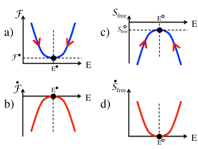
Figure 1: Graphical illustration of extremal and stability properties of equilibrium and non-equilibrium (NEQ) systems. For an equilibrium system, the free energy in a) takes its minimal value ${\cal F}^{\bullet}$ given by Eq. (32) at the equilibrium value of the covariance matrix $E^{\bullet}$, determined by Eq. (31). The free energy production $\dot{\cal F}$ in b) is negative and vanishes at the equilibrium state, see Eq. (65). This means that the system is stable with respect to perturbations and flows towards the equilibrium state, as indicated by red arrows in a). For a NEQ system, the free entropy ${\cal S}_{\rm free}(t)$ in c) takes its maximal value ${\cal S}_{\rm free}^{\circ}$ at the stationary value of the covariance matrix $E^{\circ}$. The free entropy production $\dot{\cal S}_{\rm free}(t)$ in d) is positive and vanishes in the stationary state. This means that the system is stable with respect to perturbations and flows towards the NEQ stationary state, as indicated by red arrows in c).

IV Truly Non-Equilibrium Systems

IV.1 Extremal and stability properties of the free entropy

We remark that the word non-equilibrium (NEQ) typically refers to two very different situations: For a NEQ system, i.e. when the Lyapunov-Boltzmann condition Eq. (37) is not satisfied, the stationary distribution is a NEQ stationary distribution, which is characterized by a non-vanishing positive entropy production. For such a system an equilibrium distribution does not exist. An equilibrium system is one where the Lyapunov-Boltzmann condition Eq. (37) is satisfied, but even such a system is off equilibrium as long as it has not settled in its stationary equilibrium distribution.

Obviously, it is not possible to use the constitutive equilibrium dynamic equations (66), (67) and (68) in the NEQ case, because of the appearance of the equilibrium temperature $T$. The temperature can be trivially eliminated by introducing a modified thermodynamic potential, which is called the free entropy and which is, for the equilibrium scenario using Eqs. (III.1), (28) and (31), given by

$$\frac{{\cal S}_{\rm free}(t)}{k_{B}}\equiv-\frac{{\cal F}(t)}{k_{B}T}=\frac{{\cal S}(t)}{k_{B}}-\frac{E^{\bullet-1}_{ij}E_{ij}(t)}{2}-\frac{E^{\bullet-1}_{ij}\langle z_{i}(t)\rangle\langle z_{j}(t)\rangle}{2}.$$ (69)

As mentioned before, the equilibrium free entropy had been originally introduced by Massieu in 1869 Callen (1985); Balian (2017) and the advantage of this functional was already recognized by Planck Planck (1945) and Schrödinger Schrödinger (1964). The free entropy concept is particularly useful in the current NEQ setting, since for the NEQ systems we will consider there is no unique temperature.

In fact, the free entropy concept allows for straightforward generalization to the NEQ case. For this we replace $E^{\bullet-1}_{ij}$ in Eq. (69) by $E^{\circ-1}_{ij}$, after which we obtain the NEQ version of the free entropy

$$\frac{{\cal S}_{\rm free}(t)}{k_{B}}=\frac{{\cal S}(t)}{k_{B}}-\frac{E^{\circ-1}_{ij}E_{ij}(t)}{2}-\frac{E^{\circ-1}_{ij}\langle z_{i}(t)\rangle\langle z_{j}(t)\rangle}{2}.$$ (70)

Note that the entropy production in the stationary NEQ state, which for suitably chosen friction and random strength matrices can be described as being due to heat fluxes in and out of heat reservoirs, is, as illustrated in Eq. (1), not included in the free entropy, but will be discussed in Section IV.2. Clearly, for an equilibrium system, for which $E^{\circ-1}_{ij}=E^{\bullet-1}_{ij}=H_{ij}/(k_{B}T)$, the general expression Eq. (70) reduces to the equilibrium expression Eq. (69). Similar functionals, which in a NEQ stationary state are extremal, were derived previously Graham and Haken (1971); Schlögl (1971); Procaccia and Levine (1976); Schnakenberg (1976); Kwon et al. (2005); Esposito et al. (2007); Ge (2009); Ge and Qian (2010); Qian (2013, 2015), in Appendix G we show that the free entropy expression Eq.(70) is equivalent to the Kullback-Leibler entropy Kullback and Leibler (1951); Schlögl (1971). Our model differs from previous approaches in that the definition of separate friction and random strength matrices will allow us to describe the coupling to multiple heat baths with different well-defined temperatures.

Using the free entropy, the constitutive dynamic equations (66), (67) and (68) can be rewritten as

$$\dot{\cal S}(t)=2C_{ij}\frac{\partial{\cal S}_{\rm free}(t)/k_{B}}{\partial E_{ij}},$$ (71)

$$\dot{E}_{ij}(t)= 2A_{ik}E^{\circ}_{kl}\frac{\partial{\cal S}_{\rm free}(t)/k_{B}}{\partial E_{lm}}E_{jm}$$ (72)

$$+2A_{jk}E^{\circ}_{kl}\frac{\partial{\cal S}_{\rm free}(t)/k_{B}}{\partial E_{lm}}E_{mi},$$

$$\langle\dot{z}_{i}(t)\rangle=A_{ik}E^{\circ}_{kl}\frac{\partial{\cal S}_{\rm free}(t)/k_{B}}{\partial\langle z_{l}\rangle},$$ (73)

where the temperature has obviously (and trivially) disappeared. When Eq.(70) is used in conjunction with the constitutive dynamic equations (71), (72) and (73), the exact dynamic evolution equations (derived for general NEQ systems) Eqs. (48), (56) and (16) are reproduced, this independently confirms the validity of the expression Eq. (70).

We next show that the free entropy has very similar properties for NEQ systems as the free energy has for equilibrium systems, namely ${\cal S}_{\rm free}(t)$ is extremal and in fact maximal in the stationary NEQ state and the stationary state is stable in the sense that $\dot{\cal S}_{\rm free}(t)\geq 0$. For this we basically repeat the steps leading to the minimal condition of the free energy Eq. (35). The extremum of ${\cal S}_{\rm free}(t)$ is given by $\langle\vec{z}(t)\rangle=0$ and determined by

$$\frac{\partial{\cal S}_{\rm free}(t)/k_{B}}{\partial E_{ij}}=E^{-1}_{ji}(t)/2-E^{\circ-1}_{ji}/2=0,$$ (74)

the solution of which yields the time-independent stationary distribution, i.e. $E_{ij}(t)=E^{\circ}_{ij}$. With the stationary covariance matrix $E^{\circ}_{ij}$ many observables can be calculated, for example the internal energy follows according to Eq. (III.1). The stationary free entropy is given by

$${\cal S}^{\circ}_{\rm free}/k_{B}=(1/2)\ln[(2\pi)^{2N}\det E^{\circ}].$$ (75)

The second derivative of the free entropy is given by

$$\frac{\partial^{2}{\cal S}_{\rm free}(t)/k_{B}}{\partial E_{kl}\partial E_{ij}}=-E^{-1}_{ik}(t)E^{-1}_{lj}(t)/2.$$ (76)

Around the stationary state $E_{ij}=E^{\circ}_{ij}$ the free entropy thus is to second order given by

$${\cal S}_{\rm free}(t)/k_{B}-{\cal S}^{\circ}_{\rm free}/k_{B}\simeq$$ (77)

$$E^{\circ-1}_{ik}E^{\circ-1}_{lj}(E_{ij}(t)-E^{\circ}_{ij}k_{B}T)(E_{kl}(t)-E^{\circ}_{kl}k_{B}T)/2,$$

which is positive since $E^{\circ-1}$ is symmetric and positive definite (the general proof for this is given in Appendix C).

The free entropy production follows from Eq. (70) by taking a time derivative as

$$\frac{\dot{\cal S}_{\rm free}(t)}{k_{B}}=\frac{\dot{\cal S}(t)}{k_{B}}-\frac{E^{\circ-1}_{ij}\dot{E}_{ij}(t)}{2}-E^{\circ-1}_{ij}\langle\dot{z}_{i}(t)\rangle\langle z_{j}(t)\rangle.$$ (78)

Using our previous results for $\dot{\cal S}(t)$, Eq. (48), for $\dot{E}_{ij}(t)$, Eq. (56), and for $\langle\dot{z}_{i}(t)\rangle$, Eq. (16), we arrive after a few intermediate steps at

$${\cal\dot{S}}_{\rm free}(t)/k_{B}=\langle z_{j}(t)\rangle E^{\circ-1}_{ji}A_{ik}\langle z_{k}(t)\rangle\hskip 28.45274pt$$ (79)

$$+C_{km}[E^{\circ-1}_{ml}-E^{-1}_{ml}(t)]E_{lj}(t)[E^{\circ-1}_{jk}-E^{-1}_{jk}(t)].$$

The quadratic form of this expression shows that in the stationary state, defined by $E_{kj}(t)=E^{\circ}_{kj}$ and $\langle z_{k}(t)\rangle=0$, the free entropy production of the system vanishes. More importantly, from the fact that $E^{\circ}$, $C$ and $E$ are symmetric matrices that are semi-positive-definite or positive-definite, it follows that the free entropy does not decrease in time, i.e.

$${\cal\dot{S}}_{\rm free}(t)\geq 0$$ (80)

in all generality, this means that the stationary NEQ distribution is stable with respect to perturbations, the proof is given in Appendix C. In writing Eq. (80) we have used that the first term of Eq. (79) is not negative since the product of the two positive-definite matrices $A$ and $E^{\circ}$ is also positive-definite, where positive definiteness of the asymmetric matrix $A$ is equivalent to demanding that all eigenvalues of the symmetric part of $A$ are positive, which is more restrictive than the condition that the eigenvalues of $A$ have all positive real components, as required for the existence of a stationary state in Sect. II.2. This result is here derived for interacting many body systems described by quadratic Hamiltonians and is graphically illustrated in Fig. 1. Figure 1c) shows that the free entropy ${\cal S}_{\rm free}(t)$ is maximal at the stationary distribution defined by $E_{kj}(t)=E^{\circ}_{kj}$ and $\langle z_{k}(t)\rangle=0$, which follows from Eq. (77). Figure 1d) shows that the time derivative of the free entropy ${\cal\dot{S}}_{\rm free}(t)$ is positive except at the stationary distribution where it vanishes, as follows from Eq. (79). This indicates that the system flows monotonically towards the stationary state, as indicated by the red arrows in Fig. 1c).

The free entropy maximization principle applies to NEQ and equilibrium systems alike. On the one hand this allows to treat NEQ and equilibrium systems within a unified framework and thereby eliminates a disturbing schism in the description of these systems. On the other hand, the usage of the free entropy, which does not include the stationary reservoir entropy production (which is related to the so-called house-keeping entropy Oono and Paniconi (1998); Hatano and Sasa (2001); Speck and Seifert (2005) and increases linearly in time in a stationary NEQ state, see Eq. (1) and as discussed in the next section), brings a significant methodological advantage over early approaches to NEQ systems, according to which stationary NEQ states are defined by an extremum of the total entropy production (including the reservoirs) and stability criteria invoke the time derivative of the entropy production, i.e. the second time derivative of the total entropy de Groot and Mazur (1962). The connection between the free entropy production (excluding the reservoirs) and the total entropy production (including the reservoirs) is discussed in the Conclusions and also in Appendix H.

IV.2 Stationary entropy production for particles coupled to temperature reservoirs

The calculations so far were completely general and no restrictions on the type of the Hamiltonian matrix $H$, the friction matrix $\Gamma$ and the random correlation matrix $C$ were imposed. To gain insight into the entropy production of the reservoirs, denoted by $\dot{\cal S}_{\rm res}(t)$, we need to restrict the discussion to Newtonian systems, meaning that in the Hamiltonian the spatial and momentum coordinates decouple and the kinetic energy is diagonal. This will allow to ascribe well-defined temperatures to different heat baths, which will then be used to calculate the reservoir entropy production from the individual heat fluxes between the system and the heat baths. To conveniently use the symmetry of such Newtonian systems, we switch to particle indices, denoted by greek symbols, with which the Hamiltonian can be written as

$${\cal H}(\vec{y})=y_{\alpha}H_{\alpha\epsilon}y_{\epsilon}/2.$$ (81)

Here we introduced the particle state vector

$$y_{\alpha}(t)=(x_{\alpha}(t),p_{\alpha}(t))^{T}$$ (82)

where $x_{\alpha}(t)$ and $p_{\alpha}(t)$ are the position and the momentum of particle $\alpha$. The $N\times N$ entries of the Hamiltonian matrix $H_{\alpha\epsilon}$ each consist of $2\times 2$ matrices. These sub matrices are expanded in terms of the matrices

$$u=\begin{pmatrix}0&1\\ -1&0\\ \end{pmatrix},\,\,\,\,s=\begin{pmatrix}1&0\\ 0&0\\ \end{pmatrix},\,\,\,\,r=\begin{pmatrix}0&0\\ 0&1\\ \end{pmatrix}.$$ (83)

From the matrix products

$$us=ru=\begin{pmatrix}0&0\\ -1&0\\ \end{pmatrix},\,\,\,\,ur=su=\begin{pmatrix}0&1\\ 0&0\\ \end{pmatrix}$$ (84)

it is easily seen that all $2\times 2$ matrices can be expanded in terms of the four matrices $s$, $r$, $us$ and $ur$, which thus form a convenient complete set. We will make in the following repeated use of the properties

$$s^{2}=s,\,\,\,\,r^{2}=r,\,\,\,\,u^{2}=-\mathbb{1},\,\,\,\,rs=\mathbb{0}=sr.$$ (85)

The Langevin Eq. (13) can be written as

$$\dot{y}_{\alpha}(t)=-A_{\alpha\epsilon}y_{\epsilon}(t)+\Phi_{\alpha\epsilon}F_{\epsilon}(t).$$ (86)

where $A_{\alpha\epsilon}$ is given by

$$A_{\alpha\epsilon}=-U_{\alpha\gamma}H_{\gamma\epsilon}+\Gamma_{\alpha\epsilon}$$ (87)

and $U_{\alpha\gamma}$ can be written as $U_{\alpha\gamma}=u\delta_{\alpha\gamma}$. The Hamiltonian matrix is for Newtonian systems given by

$$H_{\alpha^{\prime}\epsilon}=sh_{\alpha^{\prime}\epsilon}+r\delta_{\alpha^{\prime}\epsilon}/m_{\alpha^{\prime}}$$ (88)

where $h_{\alpha\epsilon}$ is a general $N\times N$ symmetric interaction matrix that only acts on positional degrees of freedom (and thus is multiplied by the matrix $s$) and the second term is the kinetic energy which is diagonal in the momentum degrees of freedom (and thus is multiplied by the matrix $r$) and $m_{\alpha^{\prime}}$ is the mass of particle $\alpha^{\prime}$. Note that the primed index $\alpha^{\prime}$ is not summed over. From the product properties of the $2\times 2$ matrices the inverse Hamiltonian matrix follows as

$$H^{-1}_{\alpha^{\prime}\epsilon}=sh^{-1}_{\alpha^{\prime}\epsilon}+r\delta_{\alpha^{\prime}\epsilon}m_{\alpha^{\prime}}.$$ (89)

To allow for a clear definition of reservoir temperatures, we will in the remainder treat momentum-diagonal friction, for which the friction matrix $\Gamma$ is reduced to the momenta entries as

$$\Gamma_{\alpha^{\prime}\epsilon}=r\gamma_{\alpha^{\prime}\epsilon}/m_{\alpha^{\prime}}$$ (90)

and where the matrix $\gamma_{\alpha^{\prime}\epsilon}$ is diagonal and given by $\gamma_{\alpha^{\prime}\epsilon}=\delta_{\alpha^{\prime}\epsilon}\gamma_{\alpha^{\prime}}$, where $\gamma_{\alpha^{\prime}}$ is the friction coefficient of particle $\alpha^{\prime}$. The Lyapunov-Boltzmann condition Eq. (37) in terms of particle indices reads

$$2C^{\bullet}_{\alpha\epsilon}/(k_{B}T)=\Gamma_{\alpha\gamma}H_{\gamma\epsilon}^{-1}+\Gamma_{\epsilon\gamma}H_{\gamma\alpha}^{-1},$$ (91)

which, using Eqs. (89) and (90) and the matrix product properties Eq. (85), leads to

$$C^{\bullet}_{\alpha^{\prime}\epsilon}=r\delta_{\alpha^{\prime}\epsilon}\gamma_{\alpha^{\prime}}k_{B}T,\hskip 14.22636pt\Phi^{\bullet}_{\alpha^{\prime}\epsilon}=r\phi^{\bullet}_{\alpha^{\prime}\epsilon}=r\delta_{\alpha^{\prime}\epsilon}\sqrt{\gamma_{\alpha^{\prime}}k_{B}T}.$$ (92)

These expressions show that the random correlation and random strength matrices are diagonal in the particle indices and proportional to $r$ and thus only couple momentum degrees to each other. The NEQ generalization of Eq. (92) for reservoirs with different temperatures reads

$$C_{\alpha^{\prime}\epsilon}=r\gamma_{\alpha^{\prime}}\delta_{\alpha^{\prime}\epsilon}/\beta_{\alpha^{\prime}},\hskip 28.45274pt\Phi_{\alpha^{\prime}\epsilon}=r\delta_{\alpha^{\prime}\epsilon}\sqrt{\gamma_{\alpha^{\prime}}/\beta_{\alpha^{\prime}}},$$ (93)

where $\beta_{\alpha^{\prime}}=1/(k_{B}T_{\alpha^{\prime}})$ denote the different inverse thermal energies of reservoirs, each characterized by a temperature $T_{\alpha^{\prime}}$. The expressions Eq. (93) are central to our paper as they define the NEQ model we are using to derive all following results.

To calculate an explicit expression for the reservoir entropy production we multiply the Langevin equation (86) for the momentum component $p_{\alpha}(t)$ by $p_{\alpha}(t)$ and use Eqs. (87) and (88) to obtain

$$p_{\alpha^{\prime}}(t)\dot{p}_{\alpha^{\prime}}(t)=d(p^{2}_{\alpha^{\prime}}(t))/(2dt)=\hskip 110.96556pt$$ (94)

$$-p_{\alpha^{\prime}}(t)h_{\alpha^{\prime}\epsilon}x_{\epsilon}(t)-p_{\alpha^{\prime}}(t)\gamma_{\alpha^{\prime}}p_{\alpha^{\prime}}(t)/m_{\alpha^{\prime}}+p_{\alpha^{\prime}}(t)\Phi_{\alpha^{\prime}\alpha^{\prime}}F_{\alpha^{\prime}}(t),$$

where we again note that the primed index $\alpha^{\prime}$ is not summed over. From this expression the average heating rate of the system due to reservoir $\alpha^{\prime}$, i.e. the work performed by the random force per unit time, the last term in Eq. (94), minus the friction work dissipated by the particle $\alpha^{\prime}$ per unit time, the second-last term in Eq. (94), turns out to be

$$\dot{Q}_{\alpha^{\prime}}(t) =\Phi_{\alpha^{\prime}\alpha^{\prime}}\langle p_{\alpha^{\prime}}(t)F_{\alpha^{\prime}}(t)\rangle/m_{\alpha^{\prime}}-\gamma_{\alpha^{\prime}}\langle p_{\alpha^{\prime}}(t)p_{\alpha^{\prime}}(t)\rangle/m^{2}_{\alpha^{\prime}}$$ (95)

$$=\frac{1}{2m_{\alpha^{\prime}}}\frac{{\rm d}\langle p^{2}_{\alpha^{\prime}}(t)\rangle}{{\rm d}t}+h_{\alpha^{\prime}\epsilon}\langle p_{\alpha^{\prime}}(t)x_{\epsilon}(t)\rangle/m_{\alpha^{\prime}}.$$

Since the last line of Eq. (95) is nothing but the time derivative of the sum of the kinetic and potential energies of particle $\alpha^{\prime}$, we see that the reservoir heating rate $\dot{Q}_{\alpha^{\prime}}(t)$ balances the particle energy at each instance of time (a clear consequence of the quadratic Hamiltonian approximation). For the entropy production of all reservoirs $\dot{\cal S}_{\rm res}(t)$ we thus obtain from Eq. (95) the expression

$$\frac{\dot{\cal S}_{\rm res}(t)}{k_{B}}\equiv-\beta_{\alpha}\dot{Q}_{\alpha}(t)=-\frac{\beta_{\alpha}}{2m_{\alpha}}\frac{{\rm d}\langle p^{2}_{\alpha}(t)\rangle}{{\rm d}t}-\frac{\beta_{\alpha}h_{\alpha\epsilon}}{m_{\alpha}}\langle p_{\alpha}x_{\epsilon}\rangle.$$ (96)

We now replace momenta by velocities $v_{\alpha^{\prime}}(t)=p_{\alpha^{\prime}}(t)/m_{\alpha^{\prime}}$. From the fact that in the stationary state

$$\frac{\rm d}{{\rm d}t}\langle x_{\alpha}x_{\epsilon}\rangle^{\circ}=\langle x_{\alpha}v_{\epsilon}\rangle^{\circ}+\langle v_{\alpha}x_{\epsilon}\rangle^{\circ}=0$$ (97)

and ${\rm d}\langle v^{2}_{\alpha}\rangle^{\circ}/{\rm d}t=0$ and using that $h_{\alpha\epsilon}$ is symmetric, we obtain for the reservoir entropy production in the stationary state

$$\dot{\cal S}_{\rm res}^{\circ}/k_{B}=-\beta_{\alpha}h_{\alpha\epsilon}\langle x_{\epsilon}v_{\alpha}\rangle^{\circ}=\frac{1}{2}h_{\alpha\epsilon}\langle x_{\epsilon}v_{\alpha}\rangle^{\circ}(\beta_{\epsilon}-\beta_{\alpha}).$$ (98)

This expression shows that one necessary condition for a non-zero stationary reservoir entropy production is that reservoirs have different temperatures. Other necessary conditions are a non-vanishing stationary position-velocity coupling $\langle x_{\epsilon}v_{\alpha}\rangle^{\circ}$, which for Newtonian Hamiltonian systems is only obtained off equilibrium, and a non-vanishing interaction strength $h_{\alpha\epsilon}$. To obtain explicit results for the stationary reservoir entropy production we need to calculate the position-velocity correlations $\langle x_{\epsilon}v_{\alpha}\rangle^{\circ}$, which do not vanish even in the overdamped massless limit for a NEQ system. For this a systematic perturbative scheme is introduced in the next section.

IV.3 Perturbative solution of the Lyapunov equation

The solution of the Lyapunov equation (21) for $N$ particles described by a state vector with $2N$ components consists of determining all $2N(2N+1)/2$ entries of the symmetric covariance matrix $E$. The calculation is cumbersome even for only $N=2$ particles Netz (2018). Here we introduce a systematic expansion of the Lyapunov equation with the particles mass as the perturbation parameter, which employs a projection of the matrix equations onto the complete set of $2\times 2$ matrices Eqs. (83) and (84) introduced in the previous section. This expansion is subtle, since the leading-order result for the covariance matrix in the limit $m_{\alpha}\rightarrow 0$ is not obtained by taking this limit upfront in the Langevin equation. In fact, the overdamped limit is commonly obtained by setting $m_{\alpha}=0$ in the Langevin equation Risken (1984), which correctly describes the long-time particle dynamics but obviously misses the short-time ballistic particle dynamics and leads to divergent instantaneous particle velocities. Since we need position-velocity correlations in order to estimate the entropy production according to Eq. (98), it is advisable to keep velocities to leading order as $m_{\alpha}\rightarrow 0$. As turns out, position-velocity correlations that result from the perturbation calculation stay finite even in the $m_{\alpha}\rightarrow 0$ limit.

To proceed, we expand the covariance matrix as

$$E_{\alpha\beta}=\langle x_{\alpha}x_{\beta}\rangle s+\langle p_{\alpha}p_{\beta}\rangle r+\langle x_{\alpha}p_{\beta}\rangle ut+\langle p_{\alpha}x_{\beta}\rangle us$$ (99)

and insert the expressions for $A$, Eq. (87), $H$, Eq. (88), $\Gamma$, Eq. (90), $C$, Eq. (93) and $E$, Eq. (99), into the Lyapunov Eq. (21). The resulting expression splits into an equation proportional to $s$ for $\alpha\neq\beta$

$$0=\langle x_{\alpha}v_{\beta}\rangle^{\circ}+\langle x_{\beta}v_{\alpha}\rangle^{\circ},$$ (100)

an equation proportional to $s$ for $\alpha=\beta$

$$0=\langle x_{\alpha}v_{\alpha}\rangle^{\circ},$$ (101)

an equation proportional to $r$ for $\alpha^{\prime}\neq\beta^{\prime}$

$$0=(\gamma_{\alpha^{\prime}}m_{\beta^{\prime}}+\gamma_{\beta^{\prime}}m_{\alpha^{\prime}})\langle v_{\alpha^{\prime}}v_{\beta^{\prime}}\rangle^{\circ}$$ (102)

$$+m_{\beta^{\prime}}h_{\alpha^{\prime}\gamma}\langle x_{\gamma}v_{\beta^{\prime}}\rangle^{\circ}+m_{\alpha^{\prime}}h_{\beta^{\prime}\gamma}\langle x_{\gamma}v_{\alpha^{\prime}}\rangle^{\circ},$$

an equation proportional to $r$ for $\alpha^{\prime}=\beta^{\prime}$

$$1/\beta_{\alpha^{\prime}}=m_{\alpha^{\prime}}\langle v_{\alpha^{\prime}}v_{\alpha^{\prime}}\rangle^{\circ}+\boxed{m_{\alpha^{\prime}}h_{\alpha^{\prime}\gamma}\langle x_{\gamma}v_{\beta^{\prime}}\rangle^{\circ}/\gamma_{\alpha^{\prime}}},$$ (103)

an equation proportional to $ur$ for $\alpha^{\prime}\neq\beta^{\prime}$

$$\boxed{m_{\beta^{\prime}}\langle v_{\alpha^{\prime}}v_{\beta^{\prime}}\rangle^{\circ}}=\gamma_{\beta^{\prime}}\langle x_{\alpha^{\prime}}v_{\beta^{\prime}}\rangle^{\circ}+h_{\beta^{\prime}\gamma}\langle x_{\gamma}x_{\alpha^{\prime}}\rangle^{\circ},$$ (104)

and an equation proportional to $ur$ for $\alpha^{\prime}=\beta^{\prime}$

$$m_{\alpha^{\prime}}\langle v_{\alpha^{\prime}}v_{\alpha^{\prime}}\rangle^{\circ}=h_{\alpha^{\prime}\gamma}\langle x_{\gamma}x_{\alpha^{\prime}}\rangle^{\circ},$$ (105)

where we have converted all momenta $p_{\alpha^{\prime}}$ to velocities $v_{\alpha^{\prime}}=p_{\alpha^{\prime}}/m_{\alpha^{\prime}}$. Note that there are also two equations proportional to $us$ which however are equivalent to the equations proportional to $ur$. The limit $m_{\alpha^{\prime}}\rightarrow 0$ must be taken with care. Equation (105) shows that $\langle v_{\alpha^{\prime}}v_{\alpha^{\prime}}\rangle^{\circ}\sim m^{-1}$, which reflects the equipartition theorem in the equilibrium case, while Eq. (102) suggests that $\langle v_{\alpha}v_{\beta}\rangle^{\circ}\sim\langle x_{\alpha}v_{\beta}\rangle^{\circ}$ for $\alpha\neq\beta$. Together with Eq. (104), this suggests that $\langle v_{\alpha}v_{\beta}\rangle^{\circ}\sim\langle x_{\alpha}v_{\beta}\rangle^{\circ}\sim m^{0}$ for $\alpha\neq\beta$ and thus that these terms do not necessarily vanish in the mass-less limit $m_{\alpha}\rightarrow 0$. This in turn means that the terms in the boxes in Eqs. (103) and (104) can be treated perturbatively in an expansion in powers of $m_{\alpha}$ and can, to leading order in the particles masses, be neglected. Corrections to the leading-order results for the covariances can be systematically calculated by inserting the leading-order results for the terms in the boxes and by solving the resulting equations term-by-term in powers of the particle masses. Such a calculation of next-leading-order terms would also allow to assess the accuracy of the leading-order results, but is rather involved because for NEQ systems mixed position-velocity crosscorrelations are present, as we will show explicitly for the simple case of two coupled particles in the next section. As a main result, we conclude that while the mean-squared velocities of particles diverge in the overdamped limit, the position-velocity correlations between different particles take non-zero and finite values for NEQ systems in the overdamped limit.

V Applications

V.1 Two particles coupled to different temperature reservoirs: effective temperature concept and position/momentum localization

We now present explicit results for two particles that are described by the Newtonian Hamiltonian as defined generally in Eq. (88),

$${\cal H}=h_{11}x_{1}^{2}/2+h_{22}x_{2}^{2}/2+h_{12}x_{1}x_{2}+m_{1}v_{1}^{2}/2+m_{2}v_{2}^{2}/2$$ (106)

and which are characterized by the two diagonal friction coefficients $\gamma_{1}$ and $\gamma_{2}$ as defined in Eq. (90). The particles are coupled to two heat reservoirs characterized by inverse thermal energies $\beta_{1}$ and $\beta_{2}$ as defined in Eq. (93). This is a model system that has been considered by different researchers Filliger and Reimann (2007); Crisanti et al. (2012); Dotsenko et al. (2013); Berut et al. (2016). We here reproduce the complete covariance matrix from our previous calculationNetz (2018). By straightforward solution of the set of linear equations (100)-(105) we obtain to leading order in the particle masses

$$\langle x_{1}x_{1}\rangle^{\circ}=h_{22}d\left[\frac{1}{\beta_{1}}+\Delta\frac{h_{12}}{h_{22}}\gamma_{2}\right],$$ (107)

$$\langle x_{2}x_{2}\rangle^{\circ}=h_{11}d\left[\frac{1}{\beta_{2}}-\Delta\frac{h_{12}}{h_{11}}\gamma_{1}\right],$$ (108)

$$\langle x_{1}x_{2}\rangle^{\circ}=-\frac{h_{12}d}{2}\left[\frac{1}{\beta_{1}}+\frac{1}{\beta_{2}}+\Delta\frac{h_{11}\gamma_{2}-h_{22}\gamma_{1}}{h_{12}}\right],$$ (109)

$$\langle v_{1}v_{1}\rangle^{\circ}=\frac{1}{m_{1}}\left[\frac{1}{\beta_{1}}+\Delta\frac{h_{12}m_{1}}{\gamma_{1}}\right],$$ (110)

$$\langle v_{2}v_{2}\rangle^{\circ}=\frac{1}{m_{2}}\left[\frac{1}{\beta_{2}}-\Delta\frac{h_{12}m_{2}}{\gamma_{2}}\right],$$ (111)

$$\langle v_{1}v_{2}\rangle^{\circ}=\Delta\frac{m_{2}h_{11}-m_{1}h_{22}}{\gamma_{1}m_{2}+\gamma_{2}m_{1}},$$ (112)

$$\langle x_{1}v_{2}\rangle^{\circ}=-\langle v_{1}x_{2}\rangle^{\circ}=\Delta,$$ (113)

where $d=(h_{11}h_{22}-h^{2}_{12})^{-1}$ is the inverse determinant of the interaction matrix and the parameter

$$\Delta=\frac{h_{12}}{\gamma_{1}h_{22}+\gamma_{2}h_{11}}\left(\frac{1}{\beta_{2}}-\frac{1}{\beta_{1}}\right)$$ (114)

is a measure of the departure from equilibrium. For $\Delta=0$, i.e. in equilibrium, the covariance matrix elements are given by the inverse of the Hamiltonian matrix according to Eq. 31 and in particular the off-diagonal velocity coupling terms $\langle v_{1}v_{2}\rangle^{\circ}$ and the position-velocity correlations $\langle x_{1}v_{2}\rangle^{\circ}=-\langle v_{1}x_{2}\rangle^{\circ}$ vanish. Off equilibrium, that means for $\Delta\neq 0$, these covariances are non zero and thus the symmetry of the covariance matrix changes abruptly. The expressions in the square brackets in Eqs. (107) - (111) could in principle be used to define inverse effective temperatures for the covariance elements that are non-zero in equilibrium: inspection of the terms in the square brackets shows that they are all different. For the covariances Eqs. (112) and (113) that are proportional to $\Delta$, the effective inverse temperatures are also different and diverge as equilibrium is approached, i.e. as $\Delta\rightarrow 0$. While for one or two of the covariances an effective temperature can be defined Grosberg and Joanny (2018), consideration of the entire covariance matrix shows that the ascription of an effective temperature to a particle is not possible. This suggests that an effective temperature picture, where one assigns effective temperatures to particles, does not describe the particle statistics correctly and in particular does not characterize well the transition from equilibrium, $\Delta=0$, to NEQ, $\Delta\neq 0$. To rescue the effective temperature picture one would have to ascribe different temperatures to each covariance matrix element, which clearly is far from the usefulness of the temperature definition at equilibrium. When basing the effective temperature definition on the fluctuation-dissipation relation, as an additional effect a frequency dependence appears Hohenberg and Shraiman (1989); Cugliandolo et al. (1997); Puglisi et al. (2017); Netz (2018), which is not reflected in the effective temperatures one would obtain based on the covariance matrix elements.

As an additional illustration of NEQ effects, we calculate the mean-squared difference between the particle positions, which from Eqs. (107) - (109) is to order $m^{0}$ in the particle mass given by

$$\langle(x_{1}-x_{2})^{2}\rangle^{\circ}=\frac{\beta_{1}+\beta_{2}}{2h\beta_{1}\beta_{2}}\left[1-\left(\frac{\beta_{1}-\beta_{2}}{\beta_{1}+\beta_{2}}\right)\left(\frac{\gamma_{1}-\gamma_{2}}{\gamma_{1}+\gamma_{2}}\right)\right],$$ (115)

where we have considered two particles whose center of mass is not confined, i.e. $h_{11}=h_{22}=-h_{12}=h>0$ (note that this limit must be taken with care since the interaction matrix $h_{ij}$ is not invertible in this case). The first term is the equilibrium result which survives in the limit $\beta_{1}=\beta_{2}$. Note that when the two friction coefficients and the two temperatures are different from each other, NEQ effects modify the equilibrium result. In fact, in the limits $\beta_{1}/\beta_{2}\gg 1$ and $\gamma_{1}/\gamma_{2}\gg 1$ (or $\beta_{2}/\beta_{1}\gg 1$ and $\gamma_{2}/\gamma_{1}\gg 1$) the distance between the particles tends to zero, thus indicating positional co-localization of particles, which in equilibrium one would only obtain from strong attractive interactions between particles. Interestingly, since $\beta_{\alpha}=\gamma_{\alpha}/b_{\alpha}^{2}$, where $b_{\alpha}$ denotes the strength of the Gaussian white noise that enters the Langevin equation, we see that co-localization is automatically obtained when the friction coefficients of particles $\gamma_{\alpha}$ are modified while keeping the random strengths $b_{\alpha}$ fixed. This indicates a tendency of particles to phase separate in position space in NEQ, which is indeed obtained in mixtures of particles that are coupled to different heat baths Grosberg and Joanny (2015); Weber et al. (2016); Tanaka et al. (2017); Smrek and Kremer (2017).

A similar calculation for the mean-squared velocity difference based on Eqs. (110) - (112) gives

$$\langle(v_{1}-v_{2})^{2}\rangle^{\circ}=\frac{\beta_{1}+\beta_{2}}{m\beta_{1}\beta_{2}}\left[1-\frac{mh^{2}_{12}}{h\gamma_{1}\gamma_{2}}\left(\frac{\beta_{1}-\beta_{2}}{\beta_{1}+\beta_{2}}\right)\left(\frac{\gamma_{1}-\gamma_{2}}{\gamma_{1}+\gamma_{2}}\right)\right]$$ (116)

to order $m^{0}$ and where we used the simplifications $m=m_{1}=m_{2}$ and $h_{11}=h_{22}=h$. Also here we see that in the limit $\beta_{1}/\beta_{2}\gg 1$ and $\gamma_{1}/\gamma_{2}\gg 1$ (or $\beta_{2}/\beta_{1}\gg 1$ and $\gamma_{2}/\gamma_{1}\gg 1$) the momentum difference between the particles goes down. This is indicative of co-localization in momentum space, meaning that different particles tend to move with the same velocity. For a Newtonian Hamiltonian Eq. (88) which is diagonal in momentum space and for which momenta do not couple to positions, particle velocities are uncorrelated to each other in equilibrium. We thus conclude that the momentum localization demonstrated in Eq. (116) is a NEQ phenomenon that has no equilibrium analogue for Newtonian Hamiltonians.

V.2 Stationary entropy production for three coupled particles: Heat flux from cold to warm reservoir

We will now present an explicit solution for a system consisting of three coupled particles, as schematically visualized in Fig. 2a). Since here we are only interested in the stationary entropy production, Eq. (98), we only need to calculate the stationary velocity-position cross terms $\langle x_{\epsilon}v_{\alpha}\rangle^{\circ}$. We consider the simplified Hamiltonian

$${\cal H}=\frac{h_{1}}{2}(x_{1}-x_{2})^{2}+\frac{h_{3}}{2}(x_{2}-x_{3})^{2}+\frac{m_{1}}{2}v_{1}^{2}+\frac{m_{2}}{2}v_{2}^{2}+\frac{m_{3}}{2}v_{3}^{2}$$ (117)

where only particles 1 and 2 and particles 2 and 3 are coupled via harmonic bonds. We also assume the friction coefficients to be all the same, i.e. $\gamma_{1}=\gamma_{2}=\gamma_{3}\equiv\gamma$. The solution strategy consists in eliminating $\langle v_{\alpha^{\prime}}^{2}\rangle^{\circ}$ by inserting Eq. (105) into Eq. (103), which results in 3 equations, and solving the six equations defined by Eq. (104) by using Eqs. (100) and (101). These are nine equations for nine unknowns, it turns out that Eq. (102) is not needed. The results are to order $m^{0}$ in the particle mass given by

$$\langle x_{2}v_{3}\rangle^{\circ}=\frac{1}{6\gamma(h_{1}+h_{3})}\left[\frac{h_{1}}{\beta_{1}}+\frac{h_{1}+3h_{3}}{\beta_{2}}-\frac{2h_{1}+3h_{3}}{\beta_{3}}\right],$$ (118)

$$\langle x_{1}v_{2}\rangle^{\circ}=\frac{1}{6\gamma(h_{1}+h_{3})}\left[\frac{2h_{3}+3h_{1}}{\beta_{1}}-\frac{h_{3}}{\beta_{3}}-\frac{h_{3}+3h_{1}}{\beta_{2}}\right],$$ (119)

$$\langle x_{1}v_{3}\rangle^{\circ}=\frac{1}{\gamma\Theta}\left[\frac{h_{3}+h_{2}}{\beta_{1}}+\frac{h_{1}-h_{3}}{\beta_{2}}-\frac{h_{1}+h_{2}}{\beta_{3}}\right],$$ (120)

where we defined for convenience

$$\Theta\equiv h_{1}+2h_{2}+h_{3}+\frac{h_{2}^{2}-h_{3}^{2}}{h_{1}}+\frac{h_{2}^{2}-h_{1}^{2}}{h_{3}}.$$ (121)

Inserting these results into the expression for the entropy production Eq. (98) we obtain

$$\dot{\cal S}_{\rm res}^{\circ}/k_{B}=\frac{1}{2}h_{1}\langle x_{2}v_{1}\rangle^{\circ}(\beta_{1}-\beta_{2})+\frac{1}{2}h_{3}\langle x_{2}v_{3}\rangle^{\circ}(\beta_{3}-\beta_{2})$$

$$=\frac{1}{12\gamma(h_{1}+h_{3})}\left[h_{1}h_{3}\left(\sqrt{\frac{\beta_{1}}{\beta_{3}}}-\sqrt{\frac{\beta_{3}}{\beta_{1}}}\right)^{2}\right.\hskip 28.45274pt$$ (122)

$$+h_{1}(3h_{1}+h_{3})\left(\sqrt{\frac{\beta_{1}}{\beta_{2}}}-\sqrt{\frac{\beta_{2}}{\beta_{1}}}\right)^{2}\hskip 28.45274pt$$

$$\left.+h_{3}(3h_{3}+h_{1})\left(\sqrt{\frac{\beta_{3}}{\beta_{2}}}-\sqrt{\frac{\beta_{2}}{\beta_{3}}}\right)^{2}\hskip 28.45274pt\right].$$

Obviously, the entropy production is positive and finite in the zero mass limit if the reservoir temperatures are different and if the coupling strengths $h_{1}$ and $h_{3}$ are finite and positive.

The limiting case of $h_{3}=0$ is insightful: in this case, particle 3 becomes decoupled and we are basically left with only two coupled particles. The expression Eq. (V.2) simplifies to

$$\dot{\cal S}_{\rm res}^{\circ}/k_{B}=\frac{h_{1}}{4\gamma}\left(\sqrt{\frac{\beta_{1}}{\beta_{2}}}-\sqrt{\frac{\beta_{2}}{\beta_{1}}}\right)^{2}$$ (123)

which describes the stationary entropy production of two reservoirs of inverse temperatures $\beta_{1}$ and $\beta_{2}$ that act on two particles that are subject to friction with coefficients $\gamma$ and which are coupled by a harmonic spring of strength $h_{1}$. Obviously, also this entropy production is never negative and finite if the reservoir temperatures are different and if the coupling strength $h_{1}$ is finite.

The case of three particles that are coupled to heat reservoirs at three different temperatures allows to demonstrate as an interesting NEQ effect the pumping of heat against a temperature gradient. Before we go into the analysis, we note that this does not constitute a violation of the second law of thermodynamics but rather is a NEQ entrainment effect. To proceed, we calculate the stationary heat flux from the heat reservoir at temperature $T_{1}$ to particle 1, which according to Eqs. (95) and (119) is given by

$$\dot{Q}_{1}^{\circ}= -h_{1}\langle x_{2}v_{1}\rangle^{\circ}=h_{1}\langle x_{1}v_{2}\rangle^{\circ}$$

$$= \frac{h_{1}}{6\gamma(h_{1}+h_{3})}\left[\frac{2h_{3}+3h_{1}}{\beta_{1}}-\frac{h_{3}}{\beta_{3}}-\frac{h_{3}+3h_{1}}{\beta_{2}}\right].$$ (124)

The stationary heat flux from the heat reservoir at temperature $T_{3}$ to particle 3 is according to Eqs. (95) and (118) given by

$$\dot{Q}_{3}^{\circ}= -h_{3}\langle x_{2}v_{3}\rangle^{\circ}$$

$$= -\frac{h_{3}}{6\gamma(h_{1}+h_{3})}\left[\frac{h_{1}}{\beta_{1}}+\frac{h_{1}+3h_{3}}{\beta_{2}}-\frac{2h_{1}+3h_{3}}{\beta_{3}}\right].$$ (125)

Due to energy conservation $\dot{Q}_{2}^{\circ}=-\dot{Q}_{1}^{\circ}-\dot{Q}_{3}^{\circ}$ holds. Note that all stationary heat fluxes $\dot{Q}_{1}^{\circ}$, $\dot{Q}_{2}^{\circ}$, $\dot{Q}_{3}^{\circ}$ obviously vanish in equilibrium, i.e. when the temperatures of all heat reservoirs are the same. The flux from heat reservoir 1 according to Eq. (V.2) is negative, $\dot{Q}_{1}^{\circ}<0$, i.e. heat flows into reservoir 1, for

$$\frac{T_{3}}{T_{2}}>-1-3h_{1}/h_{3}+(2+3h_{1}/h_{3})\frac{T_{1}}{T_{2}},$$ (126)

which for equal elastic coupling strengths $h_{1}=h_{3}$ simplifies to

$$\frac{T_{3}}{T_{2}}>-4+5\frac{T_{1}}{T_{2}}.$$ (127)

The flux from heat reservoir 3 according to Eq. (V.2) is positive, $\dot{Q}_{3}^{\circ}>0$, i.e. heat flows out of reservoir 3, for

$$\frac{T_{3}}{T_{2}}>\frac{h_{1}+3h_{3}}{2h_{1}+3h_{3}}+\frac{h_{1}}{2h_{1}+3h_{3}}\frac{T_{1}}{T_{2}},$$ (128)

which for equal elastic coupling strengths $h_{1}=h_{3}$ simplifies to

$$\frac{T_{3}}{T_{2}}>4/5+\frac{T_{1}}{5T_{2}}.$$ (129)

As expected, the conditions Eqs. (126) and (128) are simultaneously satisfied, i.e. heat flows into reservoir 1 and out of reservoir 3, for

$$T_{1}<T_{2}<T_{3},$$ (130)

i.e., per unit time the heat amount $|\dot{Q}_{3}^{\circ}|$, flows from particle 3 (which is coupled to the hot heat reservoir) to particle 2 (which is coupled to the warm reservoir), and the heat amount $|\dot{Q}_{1}^{\circ}|$ flows from particle 2 to particle 1 (which is coupled to the cold reservoir).

More interestingly, the conditions Eqs. (126) and (128) can also be simultaneously satisfied for the scenario

$$T_{2}<T_{1}<T_{3}.$$ (131)

In this case there is a small range of temperatures where heat flows from particle 3 (coupled to the hot heat reservoir) to particle 2 (coupled to the cold reservoir), which is expected, but at the same time a heat amount $|\dot{Q}_{1}^{\circ}|$ flows from particle 2 (coupled to the cold reservoir) to particle 1 (coupled to the warm reservoir). A similar scenario is provided for

$$T_{1}<T_{3}<T_{2},$$ (132)

where for a small range of temperatures heat flows from particle 2 (coupled to the hot heat reservoir) to particle 1 (coupled to the cold reservoir), which is expected, but at the same time a heat amount $|\dot{Q}_{3}^{\circ}|$ flows from particle 3 (coupled to the warm reservoir) to particle 2 (coupled to the hot reservoir). This means we find situations where heat flows against the temperature gradient of the heat reservoirs that are coupled to the particles. This situation is indicated in Fig. 2b) in a phase diagram for equal elastic coupling $h_{1}=h_{3}$, in which case the simplified inequalities Eqs. (127) and (129) hold. In the phase diagram the inequalities Eqs. (127) and (129) are indicated by straight lines, and the region where Eq. (130) holds is indicated in green. The regions where the inequalities Eqs. (127) and (129) and in addition Eq. (131) or Eq. (132) hold are indicated in red. Our discussion uses the fact that any heat $\dot{Q}_{1}^{\circ}$ that is transferred to or from reservoir 1 is transferred between particles 1 and 2 via elastic interactions, likewise, any heat $\dot{Q}_{3}^{\circ}$ that is transferred to or from reservoir 3 is transferred between particles 2 and 3. In other words, we do not only know the stationary heat fluxes from the reservoirs but also the stationary energy fluxes between the particles, which is due to the simple linear topology of the elastic particle interactions as indicated in Fig. 2a).

As mentioned before, the finding of a heat flux against the reservoir temperature gradient does not violate the second law of thermodynamics. Firstly, the heat flux from the particle coupled to the cold heat bath to the particle coupled to the warm heat bath is accompanied by an even larger heat flux from the particle coupled to the hot heat bath to the particle coupled to the warm heat bath, our result for the total entropy production Eq. (V.2) is strictly positive. Secondly, heat is not transferred directly between the heat reservoirs but only between particles that are coupled to heat reservoirs. In this connection it is crucial to remember (according to our previous discussion centered around the covariance elements Eqs. (107) - (113)) that particles are not characterized by the temperature of the heat reservoir they are coupled to. Therefore, since the particles do not have well-defined effective temperatures, the second law of thermodynamics is not violated. One could be tempted to define effective temperatures based on the heat fluxes, but such a definition would be based solely on one entry of the covariance matrix, namely the off-diagonal position velocity coupling $\langle x_{\alpha}v_{\beta}\rangle^{\circ}$, and not work for other applications.

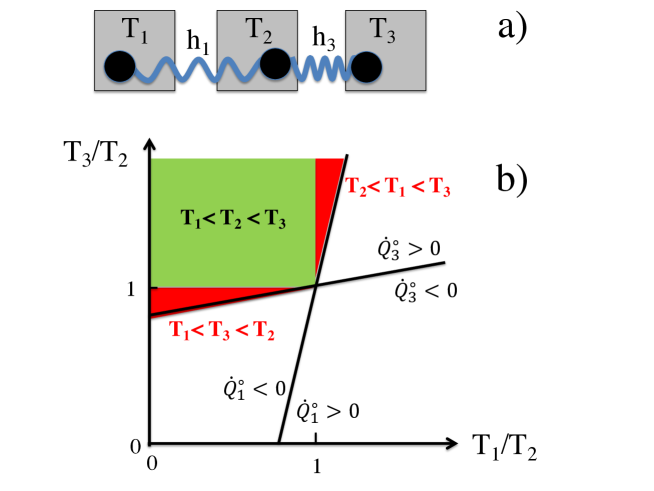
Figure 2: a) Schematic representation of three particles that interact elastically and that are coupled to heat baths with different temperatures. b) Stationary heat flux diagram for symmetric elastic couplings $h_{1}=h_{3}$, showing a colored region where heat flows from particle 3 to particle 2, i.e. $\dot{Q}_{3}^{\circ}>0$, and heat flows from particle 2 to particle 1, i.e. $\dot{Q}_{1}^{\circ}<0$. The green area denotes the temperature range $T_{1}<T_{2}<T_{3}$ and the red areas denote $T_{2}<T_{1}<T_{3}$ and $T_{1}<T_{3}<T_{2}$. The green area is the expected temperature range where heat flows from particle 3 coupled to the hot reservoir at $T_{3}$ to particle 2 coupled to the warm reservoir at $T_{2}$ and from particle 2 coupled to the warm reservoir at $T_{2}$ to particle 1 coupled to the cold reservoir at $T_{1}$. In the red areas heat flows between the particles against the temperature gradients of the heat reservoirs: In the upper red area heat flows from particle 2 coupled to the cold reservoir at $T_{2}$ to particle 1 coupled to the warm reservoir at $T_{1}$, in the lower red area heat flows from particle 3 coupled to the warm reservoir at $T_{3}$ to particle 2 coupled to the hot reservoir at $T_{2}$.

V.3 Mapping on active particles

Similar to recent calculationsDadhichi et al. (2018), we here show how active particle models can be described within the current framework of Markovian coupled particles. We want to describe a single active particle, for this we reduce the Hamiltonian Eq. (117) to two coupled massive particles and obtain

$${\cal H}=\frac{h_{1}}{2}(x_{1}-x_{2})^{2}+\frac{m_{1}}{2}v_{1}^{2}+\frac{m_{2}}{2}v_{2}^{2}.$$ (133)

By assuming the friction coefficients to be the same, i.e. $\gamma_{1}=\gamma_{2}\equiv\gamma$, and choosing two different heat bath temperatures $\beta_{1}$ and $\beta_{2}$, we obtain from Eqs. (86), (87), (88), (90) the coupled set of linear Langevin equations

$$m_{1}\,\dot{v_{1}}(t) = -\gamma v_{1}(t)-h_{1}[x_{1}(t)-x_{2}(t)]+\sqrt{\gamma/\beta_{1}}F_{1}(t),$$

$$m_{2}\,\dot{v}_{2}(t) = -\gamma v_{2}(t)-h_{1}[x_{2}(t)-x_{1}(t)]+\sqrt{\gamma/\beta_{2}}F_{2}(t).$$

The Langevin equation for the second particle is straightforwardly solved in the mass-less limit $m_{2}=0$ and gives

$$x_{2}(t)=\int_{-\infty}^{t}{\rm d}t^{\prime}{\rm e}^{-(t-t^{\prime})h_{1}/\gamma}\left[\frac{h_{1}}{\gamma}x_{1}(t^{\prime})+(\beta_{2}\gamma)^{-1/2}F_{2}(t^{\prime})\right].$$ (134)

Inserting this solution into the Langevin equation for the first particle, we obtain the generalized Langevin equation

$$m_{1}\dot{v_{1}}(t)=-\int_{-\infty}^{\infty}{\rm d}t^{\prime}\Gamma(t-t^{\prime})v_{1}(t^{\prime})+F_{R}(t).$$ (135)

The memory function that appears in Eq. (135) is given by

$$\Gamma(t)=\theta(t)\left[2\gamma\delta(t)+h_{1}{\rm e}^{-th_{1}/\gamma}\right]$$ (136)

where $\theta(t)$ denotes the Theta function with the properties $\theta(t)=1$ for $t>0$ and $\theta(t)=0$ for $t<0$, which makes the memory function single-sided. The noise $F_{R}(t)$ in Eq. (135) is given by

$$F_{R}(t)=\sqrt{\gamma/\beta_{1}}F_{1}(t)+\frac{h_{1}}{\sqrt{\beta_{2}\gamma}}\int_{-\infty}^{t}{\rm d}t^{\prime}{\rm e}^{-(t-t^{\prime})h_{1}/\gamma}F_{2}(t^{\prime})$$ (137)

and consists of the noise acting directly on the first particle and a term due to noise acting on the second particle. The latter term consists of a convolution integral because this noise is transmitted via the elastic bond of strength $h_{1}$. Defining the auto-correlation function of the random noise as $C_{\rm FF}(t)=\langle F_{R}(0)F_{R}(t)\rangle$, we obtain Netz (2018)

$$\beta_{1}C_{\rm FF}(t)=2\gamma\delta(t)+h_{1}(\beta_{1}/\beta_{2}){\rm e}^{-|t|h_{1}/\gamma}.$$ (138)

Comparing Eq. (136) and Eq. (138), we see that $\beta_{1}C_{\rm FF}(t)=\Gamma(|t|)$, a consequence of the standard fluctuation-dissipation theorem Risken (1984), only holds for $\beta_{1}=\beta_{2}$, i.e., if the two reservoir temperatures are the same. If $\beta_{1}\neq\beta_{2}$, the memory kernel $\Gamma(t)$ and the random force correlation function $C_{\rm FF}(t)$ differ, which points to FDT violation and thus to the presence of an active NEQ process. The equation of motion Eq. (135) is similar to previously studied active particle models that were shown to exhibit NEQ phase transitions Fily and Marchetti (2012); Farage et al. (2015). In fact, the active Ornstein-Uhlenbeck model is obtained by setting the exponential in the memory function Eq. (136) to zero while keeping the exponential term in the noise correlator Eq. (138). The entropy production of such active particle models has been intensely studied and debated Fodor et al. (2016); Mandal et al. (2017); Shankar and Marchetti (2018); Dabelow et al. (2019). The entropy production of the present active particle model, defined by Eq. (135) in conjunction with Eqs. (136) and (138), is given exactly by the simple expression Eq. (123); alternatively, it can be obtained directly from simulations by evaluating the position-velocity correlation functions in the general expression Eq. (98). The advantage of the present active particle model, which follows from a Newtonian Hamiltonian, is that the extremal and stability conditions in terms of the free entropy functional derived in this work are valid and not only describe the stationary NEQ distribution itself but also the approach to the stationary NEQ distribution. We hasten to add that not all active particle models can be mapped on our model, in particular models with non-Gaussian velocity distributions are not captured by our linear equations. In future work interacting active particles similar to the model derived here will be studied analytically as well as in simulations, it will be interesting to see whether the NEQ position and momentum localization effects demonstrated in Sect. V.1 also show up in those more complex systems.

VI Conclusions

In this paper we consider the approach of Hamiltonian many-body systems that are coupled to multiple heat reservoirs with different temperatures to stationary NEQ distributions. Based on the exactly calculated approach of the covariance matrix $E(t)$ to its stationary NEQ form $E^{\circ}$, we construct the functional ${\cal S}_{\rm free}(t)$ that yields the stationary covariance matrix $E^{\circ}$ at its extremum with respect to variations of $E(t)$. This function is called the free entropy, and it consists of the system distribution entropy ${\cal S}(t)$ and a term that accounts for interactions within the system, described by the Hamiltonian, and the frictional and noise coupling to the heat reservoirs.

Since in the stationary state the free entropy production by construction vanishes, as explained in Section IV.1, the difference between the free entropy production and the total entropy production is the reservoir entropy production in the stationary state, $\dot{\cal S}^{\circ}_{\rm res}$, which is constant in time. The total entropy production $\dot{\cal S}_{\rm tot}(t)$, which is the sum of the system entropy production $\dot{\cal S}(t)$ and the reservoir entropy production $\dot{\cal S}_{\rm res}(t)$, follows from Eq. (1) by differentiation as

$$\dot{\cal S}_{\rm tot}(t)=\dot{\cal S}(t)+\dot{\cal S}_{\rm res}(t)=\dot{\cal S}_{\rm free}(t)+\dot{\cal S}^{\circ}_{\rm res}.$$ (139)

Using the result in Eq. (78) we obtain the explicit expression

$$\frac{\dot{\cal S}_{\rm tot}(t)}{k_{B}}=\frac{\dot{\cal S}(t)}{k_{B}}-\frac{E^{\circ-1}_{ij}\dot{E}_{ij}(t)}{2}-E^{\circ-1}_{ij}\langle\dot{z}_{i}(t)\rangle\langle z_{j}(t)\rangle+\dot{\cal S}^{\circ}_{\rm res},$$ (140)

which consists of the system distribution entropy production $\dot{\cal S}(t)$, the stationary reservoir entropy production $\dot{\cal S}^{\circ}_{\rm res}$, and two terms that account for interactions within the system as well as the frictional and noise coupling to the environment. NEQ effects make these coupling terms differ dramatically from their equilibrium counterparts, in which case $E^{\circ-1}_{ij}$ becomes replaced by the Hamiltonian matrix $H_{ij}/(k_{B}T)$. In Appendix H we attempt to derive Eq. (139) explicitly by calculating the time-dependent reservoir entropy production $\dot{\cal S}_{\rm res}(t)$ from our explicit expressions for the time-dependent heat fluxes between the heat reservoirs and the system. We demonstrate that the heat fluxes are by themselves not sufficient to derive the reservoir entropy production $\dot{\cal S}_{\rm res}(t)$ if the reservoir temperatures are not the same, which implies that internal reservoir degrees of freedom contribute in a nonneglible manner to the reservoir entropy production for a NEQ system. The connection between the free entropy production $\dot{\cal S}_{\rm free}(t)$ (excluding the reservoirs) and the total entropy production $\dot{\cal S}_{\rm tot}(t)$ (including the reservoirs) will be reconsidered in future work using microscopic models for the heat reservoirs.

It is important to note that the reservoir entropy production in the stationary state, denoted as $\dot{\cal S}^{\circ}_{\rm res}$ and given explicitly in Eq. (98), does not depend on the time-dependent covariance matrix $E(t)$ but only on the stationary covariance matrix $E^{\circ}$, so it is a constant with respect to variations in $E(t)$; thus, the total entropy production $\dot{\cal S}_{\rm tot}(t)$ exhibits the identical extremal and stability properties as the free entropy production $\dot{\cal S}_{\rm free}(t)$. It trivially follows from Eq. (140) that the total entropy ${\cal S}_{\rm tot}(t)$ of a NEQ system increases indefinitely with time, as shown explicitly in Eq. (1), and thus is not bounded, whereas the free entropy ${\cal S}_{\rm free}(t)$ is a well-defined and finite expression even for NEQ systems. Expression Eq. (140) will be useful for various applications whenever the total entropy production of different NEQ states of a system need to be compared. The functional Eq. (140) should also allow to construct approximate methods for the description of NEQ non-linear systems as well as for NEQ phase transitions.

One advantage of the current formulation is that in the limit when all heat reservoir temperatures become equal and the NEQ system transforms into an equilibrium system, the NEQ free entropy smoothly crosses over to the equilibrium free energy divided by $-T$, which displays the standard equilibrium extremal and stability properties of a canonical system. We thus have derived a unified framework to treat NEQ systems that are coupled to heat reservoirs at different temperatures on the same footing as equilibrium systems. We have in our work restricted ourselves to one specific class of NEQ models, namely where NEQ is produced by stochastic forces with vanishing mean. Forces with a non-vanishing mean are straightforward to include and will be treated in future work.

Our approach rests on the harmonic approximation for the interaction Hamiltonian and for the friction and stochastic terms. It is not clear how to extend the present derivation to non-linear systems, here variational and perturbative methods will most likely be helpful. Clearly, a harmonic model can always be obtained from a more complex, non-linear model by a saddle-point expansion in terms of suitably defined deviatory coordinates. Our model should thus also apply to non-linear systems as long as this saddle-point approximation is justified.

Appendix A Derivation of Shannon entropy

We start from the canonical partition function

$${\cal Z}=\int{\rm d}\vec{z}{\rm e}^{-\beta{\cal H}(\vec{z})}$$ (141)

where $\beta=1/(k_{B}T)$ denotes the inverse thermal energy. Using the thermodynamic definition of the free energy ${\cal F}=-k_{B}T\ln{\cal Z}$ we can write

$${\cal F}=-k_{B}T\ln\int{\rm d}\vec{z}{\rm e}^{-\beta{\cal H}(\vec{z})}.$$ (142)

From this we obtain, using the thermodynamic definition ${\cal S}=-\partial{\cal F}/\partial T$, for the entropy

$${\cal S}=k_{B}\ln{\cal Z}+{\cal Z}^{-1}T^{-1}\int{\rm d}\vec{z}{\cal H}(\vec{z}){\rm e}^{-\beta{\cal H}(\vec{z})}.$$ (143)

From the definition of the normalized equilibrium distribution Eq.(22), we obtain

$$\beta{\cal H}(\vec{z})=-\ln\rho(\vec{z})-\ln{\cal Z},$$ (144)

which is inserted into Eq.(143) to give

$${\cal S}=-k_{B}{\cal Z}^{-1}\int{\rm d}\vec{z}{\rm e}^{-\beta{\cal H}(\vec{z})}\ln\rho(\vec{z}).$$ (145)

Using again the definition of the normalized equilibrium distribution Eq.(22), we finally obtain the Shannon expression for the entropy as

$${\cal S}/k_{B}=-\int{\rm d}\vec{z}\rho(\vec{z})\ln\rho(\vec{z}).$$ (146)

Appendix B The time dependent probability distribution is Gaussian

Here we show that the time-dependent distribution function is Gaussian and governed by the time-dependent inverse covariance matrix. The calculation holds for equilibrium as well as for NEQ systems. Given a solution $\vec{z}(t)$ of the Langevin Eq. (13), we construct the time dependent probability distribution as

$$\rho(\vec{z^{\prime}},t)=\vec{\delta}(\vec{z^{\prime}}-\vec{z}(t)).$$ (147)

Using the Fourier representation of the delta function and the time-dependent solution Eq. (14) for given initial value, we obtain

$$\rho_{F}[\vec{z^{\prime}},t,\vec{F}(\cdot)]=\int\frac{{\rm d}\vec{\omega}}{(2\pi)^{2N}}\exp\left\{-\imath\omega_{i}z_{i}^{\prime}+\imath\omega_{i}\left[\langle z_{i}(t)\rangle+\int_{0}^{t}{\rm d}t^{\prime}{\rm e}^{-(t-t^{\prime})A}_{ij}\Phi_{jk}F_{k}(t^{\prime})\right]\right\},$$ (148)

which is a functional of the random force trajectory $\vec{F}(t)$. The probability distribution is obtained by a path integral over all random force trajectories as

$$\rho(\vec{z^{\prime}},t)=\int{\cal D}\vec{F}(\cdot)P[\vec{F}(\cdot)]\rho_{F}[\vec{z^{\prime}},t,\vec{F}(\cdot)].$$ (149)

Here $P(\vec{F}(\cdot))$ is the path integral weight, which for diagonal white noise is given by

$$P[\vec{F}(\cdot))]={\cal N}_{F}^{-1}\exp\left\{-\frac{1}{4}\int{\rm d}t{\rm d}t^{\prime}F_{k}(t)\delta(t-t^{\prime})F_{k}(t^{\prime})\right\}$$ (150)

and leads to $\langle F_{i}(t)\rangle=0$ and $\langle F_{i}(t)F_{j}(t^{\prime})\rangle=2\delta_{ij}\delta(t-t^{\prime})$, where the normalization factor is given by ${\cal N}_{F}$. The path integral over the random noise in Eq.(149) can be performed and leads to the expression

$$\rho(\vec{z^{\prime}},t)=\int\frac{{\rm d}\vec{\omega}}{(2\pi)^{2N}}\exp\left\{-\imath\omega_{i}z_{i}^{\prime}+\imath\omega_{i}\langle z_{i}(t)\rangle-\omega_{i}E_{ij}(t)\omega_{j}\right\},$$ (151)

where the covariance matrix $E_{ij}(t)$ is given by Eq.(17). Performing the integral over $\vec{\omega}$ leads to

$$\rho(\vec{z^{\prime}},t)={\cal N}^{-1}(t)\exp\left\{-[z^{\prime}_{i}-\langle z_{i}(t)\rangle]E^{-1}_{ij}(t)[z^{\prime}_{j}-\langle z_{j}(t)\rangle]/2\right\},$$ (152)

with ${\cal N}$ given by Eq. (25), which is identical to the expression given in Eq. (24). Since the mean state vector $\langle z_{i}(t)\rangle$ in Eq. (152) depends according to Eq. (15) on the initial state vector $z_{i}(0)$, the time-dependent probability distribution we derived here is in fact the conditional distribution and thus corresponds to the Green’s function, this can be made explicit by rewriting Eq. (152) as

$$\rho(\vec{z^{\prime}},t| \vec{z},0)={\cal N}^{-1}(t)\exp\left\{-[z^{\prime}_{i}-{\rm e}^{-tA}_{ik}z_{k}]E^{-1}_{ij}(t)[z^{\prime}_{j}-{\rm e}^{-tA}_{jl}z_{l}]/2\right\}.$$ (153)

Appendix C Semi-positive definiteness of matrix product trace

We start from the part of the expression Eq. (64) for the free energy production rate of an equilibrium system that involves the trace of a product of four matrices,

$${\cal\dot{F}}=-C_{km}[H_{ml}-k_{B}TE^{-1}_{ml}]\frac{E_{lj}}{k_{B}T}[H_{jk}-k_{B}TE^{-1}_{jk}],$$ (154)

where we have for simplicity omitted all time dependencies. An analogous expression also appears in the free entropy production in Eq. (79). The matrix trace expressions that appear in the free energy Eq. (34) and the free entropy Eq. (77) are special cases of the more general matrix product trace we consider here.

By defining the matrix $M_{ml}=H_{ml}-k_{B}TE^{-1}_{ml}$, the expression can be written more compactly as

$$k_{B}T{\cal\dot{F}}=-C_{km}M_{ml}E_{lj}M_{jk}$$ (155)

where all matrices $C,M,E$ are symmetric and assumed to be non-defective, $E$ is positive definite, $C$ is semi-positive definite and the definiteness of $M$ (since it is the difference of two matrices) is not specified. We first diagonalize the matrix $E$ by the similarity transformation

$$EP^{E}P^{E-1}=P^{E}D^{E}P^{E-1}=P^{E}D^{E}P^{E,T}$$ (156)

where in the last step we used that $E$ is symmetric and $P^{E}$ is thus an orthogonal matrix. The matrix $D^{E}_{i^{\prime}j^{\prime}}=\delta_{i^{\prime}j}d^{E}_{i^{\prime}}$ is diagonal with diagonal elements $d^{E}_{i^{\prime}}$. We thus obtain

$$k_{B}T{\cal\dot{F}}=-C_{km}M_{ml}P_{li}D^{E}_{ij}P_{nj}M_{nk}.$$ (157)

We next define $N_{mi}=M_{ml}P_{li}$ and obtain, by using that $M$ is symmetric,

$$k_{B}T{\cal\dot{F}}=-C_{km}N_{mi}D^{E}_{ij}N_{kj}.$$ (158)

We next diagonalize the matrix $C$ by the similarity transformation

$$CP^{C}P^{C-1}=P^{C}D^{C}P^{C-1}=P^{C}D^{C}P^{C,T},$$ (159)

where $D^{C}_{i^{\prime}j^{\prime}}=\delta_{i^{\prime}j}d^{C}_{i^{\prime}}$ and obtain

$$k_{B}T{\cal\dot{F}}=-P^{C}_{kl}D^{C}_{lo}P^{C}_{mo}N_{mi}D^{E}_{ij}N_{kj}.$$ (160)

We now define $R_{oi}=P^{C}_{mo}N_{mi}$, which is equivalent to $R_{lj}=N_{kj}P^{C}_{kl}$, and thus obtain

$$k_{B}T{\cal\dot{F}}=-D^{C}_{lo}R_{oi}D^{E}_{ij}R_{lj}.$$ (161)

Now using that $D^{C}$ and $D^{E}$ are diagonal matrices we obtain

$$k_{B}T{\cal\dot{F}}=-d^{C}_{l}R_{li}d^{E}_{i}R_{li}=-d^{C}_{l}d^{E}_{i}R^{2}_{li}\leq 0,$$ (162)

where the inequality follows since the matrix elements of $R$ are real and all eigenvalues of the matrices $C$ and $E$ are not negative.

Appendix D Condition of detailed balance

Detailed balance is satisfied if the probability for a transition from a state vector $\vec{z}$ at time $t$ to a state vector $\vec{z}^{\prime}$ at time $t+\tau$ is the same as the probability for a transition from $\vec{z}^{\prime}$ at time $t$ to $\vec{z}$ at time $t+\tau$, provided that all velocities are reversed. Detailed balance is satisfied for systems that are in equilibrium and is standardly used as the definition of equilibrium de Groot and Mazur (1962). In this section we will demonstrate that the condition of detailed balance is equivalent to the condition based on the Boltzmann distribution, provided that the friction matrix is symmetric and that the stochastic field correlations satisfy certain symmetry relations. Our calculation is similar to classical derivations Van Kampen (1957a, b); Graham and Haken (1971); Schnakenberg (1976).

Using the joint probability distribution, the detailed balance condition can be written as Van Kampen (1957a, b); Graham and Haken (1971)

$$\rho(\vec{z}^{\prime},t; \vec{z},0)=\rho(W\vec{z},t;W \vec{z}^{\prime},0)$$ (163)

where $W$ is the diagonal matrix that reverses all velocities and is given by

$$W=\begin{pmatrix}1&0&0&0&\\ 0&-1&0&0&\\ 0&0&1&0&\\ 0&0&0&-1&\\ &&&&\ddots\end{pmatrix}.$$ (164)

The detailed-balance condition can be brought into its standard form by using the conditional probability, resulting in

$$\rho(\vec{z}^{\prime},t| \vec{z},0)\rho^{\circ}(\vec{z})=\rho(W\vec{z},t|W \vec{z}^{\prime},0)\rho^{\circ}(\vec{z}^{\prime}),$$ (165)

where

$$\rho^{\circ}(\vec{z})=\rho(\vec{z},t\rightarrow\infty)={\cal N}^{\circ-1}\exp\left\{-z_{i}E^{\circ-1}_{ij}z_{j}/2\right\}$$ (166)

is the stationary distribution and accordingly the time argument is omitted. The stationary normalization constant follows from Eq. (25) as ${\cal N}^{\circ}=\sqrt{(2\pi)^{2N}\det E^{\circ}}$. The conditional probability distribution $\rho(\vec{z}^{\prime},t| \vec{z},0)$, which is equivalent to the Green’s function of the stochastic problem defined by the Langevin or the Fokker-Planck equation, is explicitly given in Eq. (153) and is valid for equilibrium as well as for non-equilibrium systems. With the definition

$$\vec{z}^{\prime}=\vec{z}+\vec{\delta},$$ (167)

the covariance matrix elements according to the two sides of the detailed-balance condition Eq. (165) follow explicitly as

$$\langle\delta_{o}\delta_{p}\rangle^{\rm ls}=E_{op}(t)+(\delta_{ok}-{\rm e}^{-tA}_{ok})(\delta_{pl}-{\rm e}^{-tA}_{pl})E^{\circ}_{kl}$$ (168)

and

$$\langle\delta_{o}\delta_{p}\rangle^{\rm rs}=W_{oi}E_{ij}(t)W_{jp}$$ (169)

$$+(\delta_{ok}-W_{ol}{\rm e}^{-tA}_{lm}W_{mk})(\delta_{pn}-W_{pq}{\rm e}^{-tA}_{qr}W_{rn})E^{\circ}_{kn}.$$

Since a Gaussian distribution is completely specified by its covariance matrix, detailed balance is satisfied if $\langle\delta_{o}\delta_{p}\rangle^{\rm ls}=\langle\delta_{o}\delta_{p}\rangle^{\rm rs}$ holds. Similar to previous treatments Van Kampen (1957a, b); Graham and Haken (1971), we expand the detailed-balance condition in time. From Eq. (17) we obtain

$$E_{ij}(t)=2tC_{ij} -t^{2}(A_{ik}C_{kj}+ A_{jk}C_{ki})+{\cal O}(t^{3}).$$ (170)

To second order in $t$ we thus obtain

$$\langle\delta_{o}\delta_{p}\rangle^{\rm ls}=2tC_{op} +t^{2}(A_{ok}E^{\circ}_{kl}A_{pl}-A_{ok}C_{kp}- A_{pk}C_{ko})$$ (171)

and

$$\langle\delta_{o}\delta_{p}\rangle^{\rm rs}=2tW_{oi}C_{ij} W_{jp}$$ (172)

$$+t^{2}W_{ol}(A_{lm}W_{mn}E^{\circ}_{nt}W_{ts}A_{rs}-A_{lk}C_{kr}- A_{rk}C_{kl})W_{rp}.$$

From enforcing the detailed-balance condition term by term in powers of $t$, we obtain the two conditions

$$C_{op} =W_{oi}C_{ij} W_{jp}$$ (173)

and

$$A_{ok}E^{\circ}_{kl}A_{pl}-A_{ok}C_{kp}- A_{pk}C_{ko}$$ (174)

$$=W_{ol}(A_{lm}W_{mn}E^{\circ}_{nt}W_{ts}A_{rs}-A_{lk}C_{kr}- A_{rk}C_{kl})W_{rp},$$

which are consistent with previous results Van Kampen (1957a, b); Graham and Haken (1971). To evaluate the conditions Eqs. (173) and (174), it is useful to express all matrices as products of particle matrices and $2\times 2$ submatrices as introduced in Sect. IV.2. With this, the matrix $W$ in Eq. (164) can be written as

$$W_{\alpha\beta}=\delta_{\alpha\beta}(s-r),$$ (175)

where $s$ and $r$ are $2\times 2$ matrices defined in Eq. (83) and where greek indices number particles. To test the consequences of condition Eq. (173), we expand the random correlation matrix in the complete set of $2\times 2$ submatrices according to

$$C_{\alpha\beta}=sC_{\alpha\beta}^{\rm s}+rC_{\alpha\beta}^{\rm r}r+utC_{\alpha\beta}^{\rm ut}+usC_{\alpha\beta}^{\rm us}.$$ (176)

Inserting Eqs. (175) and (176) into Eq. (173), we obtain by using the matrix product properties Eq. (85) that $C_{\alpha\beta}^{\rm ut}=0=C_{\alpha\beta}^{\rm us}$, i.e. the random correlation matrix cannot contain components that couple momenta and positions. We will later see that this condition is indeed satisfied for a large class of Hamiltonian models.

To evaluate the consequences of the condition Eq. (174), we need to specify the symmetry of the Hamiltonian model. As in Eq. (88), the Hamiltonian matrix shall describe a Newtonian system where positions and momenta are decoupled and furthermore momentum contributions are diagonal in the particles indices,

$$H_{\alpha^{\prime}\epsilon}=sh_{\alpha^{\prime}\epsilon}+r\delta_{\alpha^{\prime}\epsilon}/m_{\alpha^{\prime}}.$$ (177)

The friction matrix is copied from Eq.(90) and only acts on momentum degrees of freedom,

$$\Gamma_{\alpha\epsilon^{\prime}}=r\gamma_{\alpha\epsilon^{\prime}}/m_{\epsilon^{\prime}},$$ (178)

in the following we explicitly allow the matrix $\gamma_{\alpha\epsilon^{\prime}}$ also to be asymmetric. Using the inverse Hamiltonian from Eq. (89) and Eq. (178), the Lyapunov-Boltzmann condition Eq. (37) yields the equilibrium random correlation matrix

$$2C_{\alpha\epsilon}/(k_{B}T)=(\gamma_{\alpha\epsilon}+\gamma_{\epsilon\alpha})r,$$ (179)

which only acts on momentum degrees of freedom. We conclude that the first detailed-balance condition Eq. (173) is automatically satisfied for a Newtonian system that is described by the Boltzmann distribution and thus satisfies the Lyapunov-Boltzmann condition Eq. (37).

We next probe condition Eq. (174). According to the definition used in the main text, in equilibrium $E^{\circ}_{kl}=E^{\bullet}_{kl}=k_{B}TH^{-1}_{kl}$ holds and thus the stationary covariance matrix $E^{\circ}_{kl}$ does not couple momentum and position coordinates, therefore condition Eq. (174) simplifies to

$$A_{ok}E^{\bullet}_{kl}A^{T}_{lp}-A_{ok}C_{kp}- C^{T}_{ok}A^{T}_{kp}$$ (180)

$$=W_{ol}(A_{lm}E^{\bullet}_{ms}A^{T}_{sr}-A_{lk}C_{kr}- C^{T}_{lk}A^{T}_{kr})W_{rp},$$

where the superindex $T$ denotes the transpose of the matrix including the $2\times 2$ submatrices. Equation (180) holds if the left side is a matrix that does not couple momenta and positions. From the expression for $A$, Eq. (87), and $U_{\alpha\gamma}=u\delta_{\alpha\gamma}$ we obtain

$$A_{\alpha^{\prime}\epsilon^{\prime}}=-ush_{\alpha^{\prime}\epsilon^{\prime}}-ur\delta_{\alpha^{\prime}\epsilon^{\prime}}/m_{\alpha^{\prime}}+r\gamma_{\alpha^{\prime}\epsilon^{\prime}}/m_{\epsilon^{\prime}}.$$ (181)

Replacing $E^{\bullet}_{kl}$ by the explicit result for $H^{-1}_{kl}$ from Eq. (89), and using the results for $C$ and $A$ from Eqs. (179) and (181) we finally obtain for the left hand side of Eq. (180)

$$rh_{\alpha^{\prime}\beta^{\prime}}+s\delta_{\alpha^{\prime}\beta^{\prime}}m_{\beta^{\prime}}^{-1}$$ (182)

$$+r\left[(\gamma_{\epsilon\alpha^{\prime}}-\gamma_{\alpha^{\prime}\epsilon})\gamma_{\beta^{\prime}\epsilon}+(\gamma_{\epsilon\beta^{\prime}}-\gamma_{\beta^{\prime}\epsilon})\gamma_{\alpha^{\prime}\epsilon}\right]m_{\epsilon}^{-1}/2$$

$$+ru(\gamma_{\alpha^{\prime}\beta^{\prime}}-\gamma_{\beta^{\prime}\alpha^{\prime}})m_{\beta^{\prime}}^{-1}/2+ur(\gamma_{\alpha^{\prime}\beta^{\prime}}-\gamma_{\beta^{\prime}\alpha^{\prime}})m_{\alpha^{\prime}}^{-1}/2.$$

For an asymmetric friction matrix $\gamma_{\alpha\beta}$, this expression contains terms that couple positions and momenta, these are the two terms proportional to $ru$ and $ur$, and therefore the second detailed-balance condition Eq. (174) is not satisfied, even if the system obeys the Boltzmann distribution. If the friction matrix $\gamma_{\alpha\beta}$ is symmetric, the terms proportional to $ru$ and $ur$ disappear and the detailed-balance condition is satisfied. We conclude that for a symmetric friction matrix the condition of detailed balance and the definition of equilibrium we use in the main text, based on the Boltzmann distribution, are equivalent. Since none of the effects we study in this paper depend on the presence of asymmetries in the friction matrix, it is permissible and convenient to use the Boltzmann definition for equilibrium, which we primarily do since it is much easier to implement. The presence of an asymmetric friction matrix means that the principle of equal actio and reactio is broken on the level of the Langevin equation, this therefore constitutes a distinct NEQ scenario.

Appendix E Condition of vanishing probability current for overdamped particle dynamics

In Sect. III.4 we show that the probability current is generally nonzero for underdamped particles. Here we consider overdamped particle motion and show that the probability current vanishes only for a symmetric friction matrix. To procced, we rewrite the equation of motion expressed in terms of particle coordinates $y_{\alpha}(t)=(x_{\alpha}(t),p_{\alpha}(t))^{T}$, Eq. (86), as a second-order differential equation as

$$m_{\alpha^{\prime}}\,\ddot{x}_{\alpha^{\prime}}(t)=-\gamma_{\alpha^{\prime}\beta}\dot{x}_{\beta}(t)-h_{\alpha^{\prime}\beta}x_{\beta}(t)+\phi_{\alpha^{\prime}\beta}F_{\beta}(t),$$ (183)

where the Hamiltonian matrix $h_{\alpha^{\prime}\beta}$ only acts on positions and the friction matrix $\gamma_{\alpha^{\prime}\beta}$ only acts on momenta. $\phi_{\alpha^{\prime}\beta}$ is the $N\times N$ random coupling strength matrix. Setting all masses $m_{\alpha}$ to zero, we obtain

$$\dot{x_{\beta}}(t)=-\gamma^{-1}_{\alpha\beta}h_{\beta\gamma}x_{\gamma}(t)+\gamma^{-1}_{\alpha\beta}\phi_{\beta\gamma}F_{\gamma}(t),$$ (184)

which we can rewrite in a form similar to Eq. (13) as

$$\dot{x}_{\alpha}(t)=-A^{\rm od}_{\alpha\beta}x_{\beta}(t)+\Phi^{\rm od}_{\alpha\beta}F_{\beta}(t),$$ (185)

where the overdamped versions of $A$ and $\Phi$ are $N\times N$ matrices given by $A^{\rm od}_{\alpha\gamma}=\gamma^{-1}_{\alpha\beta}h_{\beta\gamma}$ and $\Phi^{\rm od}_{\alpha\gamma}=\gamma^{-1}_{\alpha\beta}\phi_{\beta\gamma}$. The overdamped version of Eq. (18) is $C^{\rm od}_{kl}=\Phi^{\rm od}_{km}\Phi^{\rm od}_{lm}$. The overdamped version of the Lyapunov-Boltzmann equation Eq. (37) turns out to be

$$2C^{\rm od}_{\alpha\beta}/(k_{B}T)=\gamma^{-1}_{\alpha\beta}+\gamma^{-1}_{\beta\alpha}$$ (186)

and constitutes the relation between the random strength matrix and the friction matrix for overdamped systems. The overdamped version of the condition of vanishing probability current follows from Eq. (60) as

$$C^{\rm od}_{\alpha\beta}/(k_{B}T)=\gamma^{-1}_{\alpha\beta}$$ (187)

and, since $C^{\rm od}_{\alpha\beta}$ is symmetric by construction, can only be satisfied if the friction matrix $\gamma_{\alpha\beta}$ is symmetric. Thus, if $\gamma_{\alpha\beta}$ is not symmetric, the probability current is non-zero even if the distribution is given by the Boltzmann distribution. We conclude that the condition of vanishing probability current and the equilibrium definition we use in this paper, namely that the stationary distribution is given by the Boltzmann distribution, see Eqs. (22) and (31), are not equivalent even in the overdamped limit. In fact, the condition of vanishing probability current is more restrictive since it precludes asymmetric friction matrices, which is not necessary to obtain Boltzmann distributions. Thus, there is a class of overdamped particle models that exhibit stationary Boltzmann distributions yet that exhibit non-zero probability currents in the stationary state.

Appendix F Fluctuation-dissipation theorem

Here we demonstrate for a specific two-particle model with an asymmetric friction matrix, that the fluctuation-dissipation theorem can be satisfied even when the system, as demonstrated in Appendix D, does not obey detailed balance. To proceed, we consider a system of two massive particles that are coupled by a general friction matrix. Following the notation of Eq. (183) we write

$$m_{1}\,\ddot{x}_{1}(t)=-\gamma_{1}\dot{x}_{1}(t)-\gamma_{12}\dot{x}_{2}(t)+\phi_{1}F_{1}(t)+\phi_{12}F_{2}(t),$$ (188)

$$m_{2}\,\ddot{x}_{2}(t)=-\gamma_{2}\dot{x}_{2}(t)-\gamma_{21}\dot{x}_{1}(t)+\phi_{2}F_{2}(t)+\phi_{21}F_{1}(t).$$ (189)

Note that for ease of calculation we omit any positional couplings between the particles. Similar to the active-particle model in Sect. V.3, where the two particle positions are coupled, the Langevin equation for the second particle can be solved and gives

$$\dot{x}_{2}(t)=\int_{-\infty}^{t}{\rm d}t^{\prime}{\rm e}^{-(t-t^{\prime})\gamma_{2}/m_{2}}\left[-\frac{\gamma_{21}}{m_{2}}\dot{x}_{1}(t^{\prime})+\frac{\phi_{2}}{m_{2}}F_{2}(t^{\prime})+\frac{\phi_{21}}{m_{2}}F_{1}(t^{\prime})\right].$$ (190)

Inserting this solution into the Langevin equation for the first particle, we obtain the generalized Langevin equation

$$m_{1}\ddot{x_{1}}(t)=-\int_{-\infty}^{\infty}{\rm d}t^{\prime}\Gamma(t-t^{\prime})\dot{x}_{1}(t^{\prime})+F_{R}(t).$$ (191)

The memory function that appears in Eq. (191) is given by

$$\Gamma(t)=\theta(t)\left[2\gamma_{1}\delta(t)-\frac{\gamma_{12}\gamma_{21}}{m_{2}}{\rm e}^{-t\gamma_{2}/m_{2}}\right],$$ (192)

where $\theta(t)$ denotes the Theta function with the properties $\theta(t)=1$ for $t>0$ and $\theta(t)=0$ for $t<0$, which makes the memory function single-sided. The noise $F_{R}(t)$ in Eq. (191) is given by

$$F_{R}(t)=\phi_{1}F_{1}(t)+\phi_{12}F_{2}(t)-\int_{-\infty}^{t}{\rm d}t^{\prime}{\rm e}^{-(t-t^{\prime})\gamma_{2}/m_{2}}\left[\frac{\gamma_{12}\phi_{2}}{m_{2}}F_{2}(t^{\prime})+\frac{\gamma_{12}\phi_{21}}{m_{2}}F_{1}(t^{\prime})\right].$$ (193)

The auto-correlation function of the random noise $C_{\rm FF}(t)=\langle F_{R}(0)F_{R}(t)\rangle$ follows as

$$C_{\rm FF}(t)=2(\phi_{1}^{2}+\phi_{12}^{2})\delta(t)-[2\gamma_{12}(\phi_{2}\phi_{12}+\phi_{1}\phi_{21})-\gamma_{12}^{2}(\phi_{2}^{2}+\phi_{21}^{2})/\gamma_{2}]{\rm e}^{-|t|\gamma_{2}/m_{2}}.$$ (194)

Defining the Langevin equation in analogy to Eq. (86) in terms of the particle momenta $p_{\alpha^{\prime}}(t)=m_{\alpha^{\prime}}v_{\alpha^{\prime}}(t)$ as $\dot{p}_{\alpha}(t)=-A_{\alpha\beta}p_{\beta}(t)+\phi_{\alpha\beta}F_{\beta}(t)$ where $A_{\alpha\beta^{\prime}}=\gamma_{\alpha\beta^{\prime}}/m_{\beta^{\prime}}$ and $H_{\alpha\beta^{\prime}}=\delta_{\alpha\beta^{\prime}}/m_{\beta^{\prime}}$, we obtain from Eq. (36) the Boltzmann-Lyapunov equation

$$2C_{\alpha\beta}=2\phi_{km}\phi_{lm}=k_{B}T(\gamma_{\alpha\beta}+\gamma_{\beta\alpha}),$$ (195)

or, explicitly,

$$2\begin{pmatrix}\phi_{1}^{2}+\phi_{12}^{2}&\phi_{1}\phi_{21}+\phi_{2}\phi_{12}\\ \phi_{1}\phi_{21}+\phi_{2}\phi_{12}&\phi_{2}^{2}+\phi_{21}^{2}\end{pmatrix}=k_{B}T\begin{pmatrix}2\gamma_{1}&\gamma_{12}+\gamma_{21}\\ \gamma_{12}+\gamma_{21}&2\gamma_{2}\end{pmatrix}.$$ (196)

Provided Eq. (196) holds, it is easy to see that Eqs. (192) and Eq. (194) satisfy the fluctuation-dissipation theorem Risken (1984)

$$C_{\rm FF}(t)=k_{B}T\Gamma(|t|),$$ (197)

even if the friction matrix $\gamma_{\alpha\beta}$ is asymmetric. In contrast and as shown in Appendix D, the more restrictive detailed-balance condition is only satisfied if the friction matrix $\gamma_{\alpha\beta}$ is symmetric. This suggests that the definition of equilibrium we use in this paper, namely that the stationary distribution corresponds to the Boltzmann distribution, coincides with the fluctuation-dissipation theorem even for asymmetric $\gamma_{\alpha\beta}$. On the other hand, the detailed-balance condition is more restrictive and can only be satisfied if the friction matrix is symmetric.

Appendix G Equivalenz of free entropy and Kullback-Leibler entropy

The multidimensional expression for the Kullback-Leibler entropy reads Kullback and Leibler (1951); Schlögl (1971)

$${\cal S}_{\rm KL}=-\int{\rm d}\vec{z}\rho(\vec{z})\ln\left[\frac{\rho^{\circ}(\vec{z})}{\rho(\vec{z})}\right],$$ (198)

where the Gaussian probability distribution $\rho(\vec{z})$ and the Gaussian stationary probability distribution $\rho^{\circ}(\vec{z})$ are given by

$$\rho(\vec{z})={\cal N}^{-1}\exp\left(-z_{i}E^{-1}_{ij}z_{j}/2\right),$$ (199)

$$\rho^{\circ}(\vec{z})={\cal N^{\circ}}^{-1}\exp\left(-z_{i}E^{\circ-1}_{ij}z_{j}/2\right)$$ (200)

with the normalization constants ${\cal N}=\sqrt{(2\pi)^{2N}\det E}$ and ${\cal N}^{\circ}=\sqrt{(2\pi)^{2N}\det E^{\circ}}$. Note that we dropped all time dependencies for simplicity. Using the inequality

$$-\ln\left[\frac{\rho^{\circ}(\vec{z})}{\rho(\vec{z})}\right]\geq 1-\frac{\rho^{\circ}(\vec{z})}{\rho(\vec{z})}$$ (201)

and the fact that $\rho(\vec{z})$ and $\rho^{\circ}(\vec{z})$ are normalized, it immediately follows that

$${\cal S}_{\rm KL}\geq 0$$ (202)

and that ${\cal S}_{\rm KL}=0$ for $\rho(\vec{z})=\rho^{\circ}(\vec{z})$. A short calculation shows that also $\delta{\cal S}_{\rm KL}/\delta\rho(\vec{z})=0$ for $\rho(\vec{z})=\rho^{\circ}(\vec{z})$, thus, the Kullback-Leibler is minimal for $\rho(\vec{z})=\rho^{\circ}(\vec{z})$. Performing the Gaussian integrals in Eq. (198), one immediately obtains

$${\cal S}_{\rm KL}=E^{\circ-1}_{ij}E_{ij}/2-N-\ln\left[(2\pi)^{2N}\det E\right] /2$$

$$+\ln\left[(2\pi)^{2N}\det E^{\circ}\right] /2.$$ (203)

Comparison of the Kullback-Leibler entropy Eq. (G) with the non-equilibrium free entropy expression Eq. (70) shows that the two expressions are identical except the sign and terms that do not depend on covariance matrix elements $E_{ij}$.

Appendix H Non-stationary entropy production of heat reservoirs

We start from the expression for the time-dependent entropy production of all reservoirs Eq. (96), which is based on the result for the heat fluxes between the reservoirs and the system in Eq. (95). We recall that the calculation of the reservoir heat fluxes is based on the general Newtonian Hamiltonian as defined by Eq. (88) with diagonal momentum friction as defined by Eq. (90) and the NEQ model defined by the diagonal noise correlation matrix Eq. (93).

Using the result for the time derivative of the covariance matrix Eq. (55) together with the explicit expression for the $A$ matrix Eq. (87) and the expansion of the covariance matrix $E$ Eq. (99), we obtain for the time derivative of the squared particle momenta

$$\frac{{\rm d}\langle p^{2}_{\alpha^{\prime}}(t)\rangle}{{\rm d}t}=2C_{\alpha^{\prime}\alpha^{\prime}}-\frac{2\gamma_{\alpha^{\prime}}}{m_{\alpha^{\prime}}}\langle p^{2}_{\alpha^{\prime}}(t)\rangle-2h_{\alpha^{\prime}\epsilon}\langle p_{\alpha^{\prime}}x_{\epsilon}\rangle.$$ (204)

Inserting this into the total reservoir entropy production Eq. (96) we obtain

$$\frac{\dot{\cal S}_{\rm res}(t)}{k_{B}}=\frac{\beta_{\alpha}\gamma_{\alpha}}{m_{\alpha}}\left(\frac{\langle p^{2}_{\alpha}(t)\rangle}{m_{\alpha}}-\frac{1}{\beta_{\alpha}}\right),$$ (205)

where the non-primed index $\alpha$ is summed over. Clearly, in an equilibrium stationary state, where the kinetic energy of each particle obeys $\langle p^{2}_{\alpha}(t)\rangle/(m_{\alpha})=1/\beta_{\alpha}$ and $\beta_{\alpha}=\beta$, the entropy production vanishes. In a stationary state we can replace $\langle p^{2}_{\alpha}(t)\rangle$ by the expression Eq. (103) and thereby recover Eq. (98), so our calculation thus far is consistent. We will now test whether the stationary NEQ distribution constitutes an extremum of the total entropy production, which according to Eq. (139) is given by

$$\dot{\cal S}_{\rm tot}(t)=\dot{\cal S}(t)+\dot{\cal S}_{\rm res}(t),$$ (206)

where $\dot{\cal S}(t)$ denotes the Shannon entropy production of the system distribution Eq. (46) and $\dot{\cal S}_{\rm res}(t)$ is given by Eq. (205). As an explicit calculation shows, the derivative of the reservoir entropy production Eq. (205) with respect to the covariance matrix gives

$$\frac{\partial\dot{\cal S}_{\rm res}(t)}{\partial E_{ij}}=\Gamma_{ik}C^{-1}_{km}\Gamma_{mj},$$ (207)

which using Eqs. (90) and (93) is a diagonal matrix with momentum entries $\beta_{\alpha^{\prime}}\gamma_{\alpha^{\prime}}/m^{2}_{\alpha^{\prime}}$. For the system entropy production we obtain from Eq. (46)

$$\frac{\partial\dot{\cal S}(t)}{\partial E_{ij}}=-E^{-1}_{ik}(t)C_{km}E^{-1}_{mj}(t)$$ (208)

and thus for the total entropy

$$\frac{\partial\dot{\cal S}_{\rm tot}(t)}{\partial E_{ij}}=\Gamma_{ik}C^{-1}_{km}\Gamma_{mj}-E^{-1}_{ik}(t)C_{km}E^{-1}_{mj}(t).$$ (209)

Multiplying by $C_{li}$ we obtain

$$C_{li}\frac{\partial\dot{\cal S}_{\rm tot}(t)}{\partial E_{ij}}=\Gamma_{lk}\Gamma_{kj}-C_{li}E^{-1}_{ik}(t)C^{-1}_{km}E^{-1}_{mj}(t),$$ (210)

which vanishes when

$$\Gamma_{lk}\Gamma_{kj}=C_{li}E^{-1}_{ik}(t)C^{-1}_{km}E^{-1}_{mj}(t)$$ (211)

holds. Taking the square root and multiplying by $E$ we obtain

$$\Gamma_{lk}E_{ki}(t)=C_{li}$$ (212)

as the equation which determines the extremum of the total entropy production. It turns out that that Eq. (212) is satisfied by the equilibrium stationary distribution $E^{\bullet}_{ki}$, therefore for an equilibrium system the total entropy production as defined in Eq. (206) is extremal in the equilibrium state.

It is easy to verify that for the stationary NEQ distribution $E^{\circ}_{ki}$ with non zero matrix elements $\langle p_{i}p_{j}\rangle^{\circ}$ and $\langle x_{i}p_{j}\rangle^{\circ}$ for $i\neq j$, and $\Gamma$ and $C$ given by Eqs. (90) and (93), Eq. (212) is not satisfied. This implies that the total entropy production Eq. (206), which is the sum of the non-stationary reservoir entropy production Eq. (96) or (205) (calculated from the heat fluxes between reservoirs and the system) and the system distribution entropy production Eq. (46), does not yield the exactly calculated stationary distribution $E^{\circ}_{ki}$ at its extremum and thus differs from the total entropy production constructed from the sum of the free entropy and the stationary reservoir entropy production according to Eq. (139). We conclude that non-stationary entropy contributions that presumably stem from internal reservoir degrees of freedom render the expressions Eqs. (96) and (205) incomplete. These internal reservoir degrees could be included by using microscopic models for the heat reservoirs.

References

- Onsager (1931) L. Onsager, Reciprocal relations in irreversible processes. i, Phys. Rev. 37, 405 (1931).
- Prigogine (1947) I. Prigogine, Etude thermodynamic des phenomene irreversibles (Desoer, Liege, 1947).
- Prigogine and Mazur (1953) I. Prigogine and P. Mazur, Sur l’extension de la thermodynamique aux phenomenes irreversibles lies aux degres de liberte internes, Physica XIX, 241 (1953).
- Lebowitz (1959) J. L. Lebowitz, Stationary nonequilibrium gibbsian ensembles, Phys. Rev. 114, 1192 (1959).
- Graham and Haken (1971) R. Graham and H. Haken, Generalized thermodynamic potential for markoff systems in detailed balance and far from thermal equilibrium, Z. Physik 243, 289 (1971).
- Schlögl (1971) F. Schlögl, On stability of steadystates, Z. Physik 243, 303 (1971).
- Procaccia and Levine (1976) I. Procaccia and R. D. Levine, Potential work: A statistical-mechanical approach for systems in disequilibrium, J. Chem. Phys. 65, 3357 (1976).
- Schnakenberg (1976) J. Schnakenberg, Network theory of microscopic and macroscopic behavior of master equation system, Rev. Mod. Phys. 48, 571 (1976).
- Oono and Paniconi (1998) Y. Oono and M. Paniconi, Steady state thermodynamics, Progress of Theoretical Physics Supplement 130, 29 (1998).
- Hatano and Sasa (2001) T. Hatano and S. I. Sasa, Steady-state thermodynamics of langevin systems, Phys. Rev. Lett. 86, 3463 (2001).
- Esposito et al. (2007) M. Esposito, U. Harbola, and S. Mukamel, Entropy fluctuation theorems in driven open systems: Application to electron counting statistics, Phys. Rev. E 76, 031132 (2007).
- Ramaswamy (2010) S. Ramaswamy, The mechanics and statics of active matter, Annu. Rev. Condens. Matter Phys. 1, 323 (2010).
- Chou et al. (2011) T. Chou, K. Mallick, and R. K. P. Zia, Non-equilibrium statistical mechanics: from a paradigmatic model to biological transport, Rep. Prog. Phys. 74, 116601 (2011).
- Seifert (2012) U. Seifert, Stochastic thermodynamics, fluctuation theorems and molecular machines, Rep. Prog. Phys. 75, 126001 (2012).
- Marchetti et al. (2013) M. C. Marchetti, J. F. Joanny, S. Ramaswamy, T. B. Liverpool, J. Prost, M. Rao, and R. A. Simha, Hydrodynamics of soft active matter, Rev. Mod. Phys. 85, 1143 (2013).
- Gnesotto et al. (2018) F. S. Gnesotto, F. Mura, J. Gladrow, and C. P. Broedersz, Broken detailed balance and non-equilibrium dynamics in living systems: a review, Rep. Prog. Phys.. 81, 066601 (2018).
- Bechinger et al. (2016) C. Bechinger, R. Di Leonardo, H. Löwen, C. Reichhardt, G. Volpe, and G. Volpe, Active particles in complex and crowded environments, Rev. Mod. Phys. 88, 045006 (2016).
- Illien et al. (2017) P. Illien, R. Golestanian, and A. Sen, ’fuelled’ motion: phoretic motility and collective behaviour of active colloids, Chem. Soc. Rev. 46, 5508 (2017).
- Netz (2018) R. R. Netz, Fluctuation-dissipation relation and stationary distribution of an exactly solvable many-particle model for active biomatter far from equilibrium, J. Chem. Phys. 148, 185101 (2018).
- Katz et al. (1983) S. Katz, J. L. Lebowitz, and H. Spohn, Phase transitions in stationary nonequilibrium states of model lattice systems, Phys. Rev. B 28, 1655 (1983).
- Krug (1991) J. Krug, Boundary-induced phase transitions in driven diffusive systems, Phys. Rev. Lett. 67, 1882 (1991).
- Schmittmann and Zia (1998) B. Schmittmann and R. K. P. Zia, Driven diffusive systems. an introduction and recent developments, Phys. Rep. 301, 45 (1998).
- Dzubiella et al. (2002) J. Dzubiella, G. P. Hoffmann, and H. Löwen, Lane formation in colloidal mixtures driven by an external field, Phys. Rev. E 65, 021402 (2002).
- Netz (2003) R. R. Netz, Conduction and diffusion in two-dimensional electrolytes, Europhys. Lett. 63, 616 (2003).
- Kumar et al. (2014) N. Kumar, H. Soni, S. Ramaswamy, and A. K. Sood, Flocking at a distance in active granular matter, Nature Communications 5, 4688 (2014).
- Bertin et al. (2006) E. Bertin, M. Droz, and G. Grégoire, Boltzmann and hydrodynamic description for self-propelled particles, Phys. Rev. E 74, 022101 (2006).
- Theurkauff et al. (2012) I. Theurkauff, C. Cottin-Bizonne, J. Palacci, C. Ybert, and L. Bocquet, Dynamic clustering in active colloidal suspensions with chemical signaling, Phys. Rev. Lett. 108, 268303 (2012).
- Golestanian (2012) R. Golestanian, Collective behavior of thermally active colloids, Phys. Rev. Lett. 108, 038303 (2012).
- Speck et al. (2014) T. Speck, J. Bialke, A. M. Menzel, and H. Löwen, Effective cahn-hilliard equation for the phase separation of active brownian particles, Phys. Rev. Lett. 112, 218304 (2014).
- Ginot et al. (2015) F. Ginot, I. Theurkauff, D. Levis, C. Ybert, L. Bocquet, L. Berthier, and C. Cottin-Bizonne, Nonequilibrium equation of state in suspensions of active colloids, Phys. Rev. X 5, 011004 (2015).
- Grosberg and Joanny (2015) A. Y. Grosberg and J. F. Joanny, Nonequilibrium statistical mechanics of mixtures of particles in contact with different thermostats, Phys. Rev. E 92, 032118 (2015).
- Weber et al. (2016) S. N. Weber, C. A. Weber, and E. Frey, Binary mixtures of particles with different diffusivities demix, Phys. Rev. Lett. 116, 058301 (2016).
- Tanaka et al. (2017) H. Tanaka, A. A. Lee, and M. P. Brenner, Hot particles attract in a cold bath, Phys. Rev. Fluids 2, 043103 (2017).
- Smrek and Kremer (2017) J. Smrek and K. Kremer, Small activity differences drive phase separation in active-passive polymer mixtures, Phys. Rev. Lett. 118, 098002 (2017).
- Chari et al. (2019) S. S. N. Chari, C. Dasgupta, and P. K. Maiti, Scalar activity induced phase separation and liquid-solid transition in lennard-jones system, Soft Matter 15, 7275 (2019).
- Sokolov et al. (2007) A. Sokolov, I. S. Aranson, J. O. Kessler, and R. E. Goldstein, Concentration dependence of the collective dynamics of swimming bacteria, Phys. Rev. Lett. 98, 158102 (2007).
- Suzuki and Bausch (2017) R. Suzuki and A. R. Bausch, The emergence and transient behaviour of collective motion in active filament systems, Nature Communications 8, 41 (2017).
- Helbing (2001) D. Helbing, Traffic and related self-driven many-particle systems, Rev. Mod. Phys. 73, 1067 (2001).
- Wolgemuth et al. (2000) C. W. Wolgemuth, T. R. Powers, and R. E. Goldstein, Twirling and whirling: Viscous dynamics of rotating elastic filaments, Phys. Rev. Lett. 84, 1623 (2000).
- Wada and Netz (2009) H. Wada and R. R. Netz, Plectoneme creation reduces the rotational friction of a polymer, Europhys. Lett. 87, 38001 (2009).
- Agarwal (1972) G. S. Agarwal, Fluctuation-dissipation theorems for systems in non-thermal equilibrium and applications, Z. Physik 252, 25 (1972).
- Hohenberg and Shraiman (1989) P. C. Hohenberg and B. I. Shraiman, Chaotic behavior of an extended system, Physica D 37, 109 (1989).
- Cugliandolo et al. (1997) L. F. Cugliandolo, J. Kurchan, and L. Peliti, Energy flow, partial equilibration, and effective temperatures in systems with slow dynamics, Phys. Rev. E 55, 3898 (1997).
- Speck and Seifert (2006) T. Speck and U. Seifert, Restoring a fluctuation-dissipation theorem in a nonequilibrium steady state, Europhys. Lett. 74, 391 (2006).
- Xu and O’Hern (2005) N. Xu and C. S. O’Hern, Effective temperature in athermal systems sheared at fixed normal load, Phys. Rev. Lett. 94, 055701 (2005).
- Ilg and Barrat (2007) P. Ilg and J. L. Barrat, From single-particle to collective effective temperatures in an active fluid of self-propelled particles, Europhys. Lett. 111, 26001 (2007).
- Krüger and Fuchs (2009) M. Krüger and M. Fuchs, Fluctuation dissipation relations in stationary states of interacting brownian particles under shear, Phys. Rev. Lett. 102, 135701 (2009).
- Levis and Berthier (2015) D. Levis and L. Berthier, Driven activation vs. thermal activation, Europhys. Lett. 79, 60006 (2015).
- Harada and Sasa (2005) T. Harada and S. I. Sasa, Equality connecting energy dissipation with a violation of the fluctuation-response relation, Phys. Rev. Lett. 95, 130602 (2005).
- Zamponi et al. (2005) F. Zamponi, F. Bonetto, L. F. Cugliandolo, and J. Kurchan, A fluctuation theorem for non-equilibrium relaxational systems driven by external forces, J. Stat. Mech. , P09013 (2005).
- Prost et al. (2009) J. Prost, J.-F. Joanny, and J. M. R. Parrondo, Generalized fluctuation-dissipation theorem for steady-state systems, Phys. Rev. Lett. 103, 090601 (2009).
- Baiesi et al. (2009) M. Baiesi, C. Maes, and B. Wynants, Fluctuations and response of nonequilibrium states, Phys. Rev. Lett. 103, 010602 (2009).
- Seifert and Speck (2010) U. Seifert and T. Speck, Fluctuation-dissipation theorem in nonequilibrium steady states, Europhys. Lett. 89, 10007 (2010).
- Willareth et al. (2017) L. Willareth, I. M. Sokolov, Y. Roichman, and B. Lindner, Generalized fluctuation-dissipation theorem as a test of the markovianity of a system, Europhys. Lett. 118, 20001 (2017).
- Jabbari-Farouji et al. (2008) S. Jabbari-Farouji, D. Mizuno, D. Derks, G. H. Wegdam, F. C. MacKintosh, C. F. Schmidt, and D. Bonn, Effective temperatures from the fluctuation-dissipation measurements in soft glassy materials, Europhysics Letters 84, 20006 (2008).
- Gomez-Solano et al. (2009) J. R. Gomez-Solano, A. Petrosyan, S. Ciliberto, R. Chetrite, and K. Gawedzki, Experimental verification of a modified fluctuation-dissipation relation for a micron-sized particle in a nonequilibrium steady state, Phys. Rev. Lett. 103, 040601 (2009).
- Mehl et al. (2010) J. Mehl, V. Blickle, U. Seifert, and C. Bechinger, Experimental accessibility of generalized fluctuation-dissipation relations for nonequilibrium steady states, Phys. Rev. E 82, 032401 (2010).
- Martin et al. (2001) P. Martin, A. J. Hudspeth, and F. Jülicher, Comparison of a hair bundle’s spontaneous oscillations with its response to mechanical stimulation reveals the underlying active process, Proc. Nat. Acad. Sci. USA 98, 14380 (2001).
- Dinis et al. (2012) L. Dinis, P. Martin, J. Barral, J. Prost, and J.-F. Joanny, Fluctuation-response theorem for the active noisy oscillator of the hair-cell bundle, Phys. Rev. Lett. 109, 160602 (2012).
- Bohec et al. (2013) P. Bohec, F. F. Gallet, C. Maes, S. Safaverdi, P. Visco, and F. van Wijland, Probing active forces via a fluctuation-dissipation relation: Application to living cells, Europhys. Lett. 102, 50005 (2013).
- Mizuno et al. (2007) D. Mizuno, C. Tardin, C. F. Schmidt, and F. C. MacKintosh, Nonequilibrium mechanics of active cytoskeletal networks, Science 315, 370 (2007).
- Lebowitz and Spohn (1999) J. L. Lebowitz and H. Spohn, A gallavotti cohen-type symmetry in the large deviation functional for stochastic dynamics, Journal of Statistical Physics 95, 333 (1999).
- Crooks (1999) G. E. Crooks, Entropy production fluctuation theorem and the nonequilibrium work relation for free energy differences, Phys. Rev. E 60, 2721 (1999).
- Jarzynski (2000) C. Jarzynski, Hamiltonian derivation of a detailed fluctuation theorem, Journal of Statistical Physics 98, 77 (2000).
- Seifert (2005) U. Seifert, Entropy production along a stochastic trajectory and an integral fluctuation theorem, Phys. Rev. Lett. 95, 040602 (2005).
- Doi et al. (2019) M. Doi, J. Zhou, Y. Di, and X. Xu, Application of the onsager-machlup integral in solving dynamic equations in nonequilibrium systems, Phys. Rev. E 99, 063303 (2019).
- Rieder et al. (1967) Z. Rieder, J. L. Lebowitz, and E. Lieb, Properties of a harmonic crystal in a stationary nonequilibrium state, J. Math. Phys. 8, 1073 (1967).
- Zwanzig (1973) R. Zwanzig, Non linear generalized langevin equations, J. Stat. Phys. 9, 215 (1973).
- Filliger and Reimann (2007) R. Filliger and P. Reimann, Brownian gyrator: A minimal heat engine on the nanoscale, Phys. Rev. Lett. 99, 230602 (2007).
- Dadhichi et al. (2018) L. P. Dadhichi, A. Maitra, and S. Ramaswamy, Origins and diagnostics of the nonequilibrium character of active systems, Journal of Statistical Mechanics , 123201 (2018).
- Li et al. (2019) J. Li, J. M. Horowitz, T. R. Gingrich, and N. Fakhri, Quantifying dissipation using fluctuating currents, Nature Communications 15, 1666 (2019).
- Callen (1985) H. B. Callen, Thermodynamics and an Introduction to Thermostatistics (John Wiley Sons, New York, 1985).
- Balian (2017) R. Balian, Francois massieu and the thermodynamic potentials, C. R. Physique 18, 526 (2017).
- Planck (1945) M. Planck, Treatise on Thermodynamics (Dover Publications, New York, 1945).
- Schrödinger (1964) E. Schrödinger, Statistical Thermodynamics (Cambridge University Press, Cambridge, 1964).
- Biane and Speicher (2001) P. Biane and R. Speicher, Free diffusions, free entropy and free fisher information, Ann. I. H. Poincare - PR 3 7, 581 (2001).
- Voiculescu (2002) D. Voiculescu, Free entropy, Bull. London Math. Soc. 34, 257 (2002).
- Kullback and Leibler (1951) S. Kullback and R. A. Leibler, On information and sufficiency, Annals of Math. Statistics 22, 79 (1951).
- Kwon et al. (2005) C. Kwon, P. Ao, and D. J. Thouless, Structure of stochastic dynamics near fixed points, Proc. Nat. Acad. Sci. USA 102, 13029 (2005).
- Ge (2009) H. Ge, Extended forms of the second law for general time-dependent stochastic processes, Phys. Rev. E 80, 021137 (2009).
- Ge and Qian (2010) H. Ge and H. Qian, Physical origins of entropy production, free energy dissipation, and their mathematical representations, Phys. Rev. E 81, 051133 (2010).
- Qian (2013) H. Qian, A decomposition of irreversible diffusion processes without detailed balance, J. Math. Phys. 54, 053302 (2013).
- Qian (2015) H. Qian, Thermodynamics of the general diffusion process: Equilibrium supercurrent and nonequilibrium driven circulation with dissipation, Eur. Phys. J. Special Topics 224, 781 (2015).
- Speck and Seifert (2005) T. Speck and U. Seifert, Integral fluctuation theorem for the housekeeping heat, J. Phys. A: Amth. Gen. 38, L581 (2005).
- Zwanzig (1961) R. Zwanzig, Memory effects in irreversible thermodynamics, Physical Review 124, 983 (1961).
- Risken (1984) H. Risken, The Fokker-Planck Equation (Springer, Berlin, 1984).
- de Groot and Mazur (1962) S. R. de Groot and P. Mazur, Non-Equilibrium Thermodynamics (North-Holland Pub. Co., Amsterdam, 1962).
- Crisanti et al. (2012) A. Crisanti, A. Puglisi, and D. Villamaina, Nonequilibrium and information: The role of cross correlations, Phys. Rev. E 85, 061127 (2012).
- Dotsenko et al. (2013) V. Dotsenko, A. Maciolek, O. Vasilyev, and G. Oshanin, Two-temperature langevin dynamics in a parabolic potential, Phys. Rev. E 87, 062130 (2013).
- Berut et al. (2016) A. Berut, A. Imparato, A. Petrosyan, and S. Ciliberto, Theoretical description of effective heat transfer between two viscously coupled beads, Phys. Rev. E 94, 052148 (2016).
- Grosberg and Joanny (2018) A. Y. Grosberg and J. F. Joanny, Dissipation in a system driven by two different thermostats, Polymer Science, Series C 60, 118 (2018).
- Puglisi et al. (2017) A. Puglisi, A. Sarracino, and V. A., Temperature in and out of equilibrium: A review of concepts, tools and attempts, Phys. Rep. 709, 1 (2017).
- Fily and Marchetti (2012) Y. Fily and M. C. Marchetti, Athermal phase separation of self-propelled particles with no alignment, Phys. Rev. Lett. 108, 235702 (2012).
- Farage et al. (2015) T. F. F. Farage, P. Krinninger, and J. M. Brader, Effective interactions in active brownian suspensions, Phys. Rev. E 91, 042310 (2015).
- Fodor et al. (2016) E. Fodor, C. Nardini, M. E. Cates, J. Tailleur, P. Visco, and F. van Wijland, How far from equilibrium is active matter? Phys. Rev. Lett. 117, 038103 (2016).
- Mandal et al. (2017) D. Mandal, K. Klymko, and M. R. DeWeese, Entropy production and fluctuation theorems for active matter, Phys. Rev. Lett. 119, 258001 (2017).
- Shankar and Marchetti (2018) S. Shankar and M. C. Marchetti, Hidden entropy production and work fluctuations in an ideal active gas, Phys. Rev. E 98, 020604(R) (2018).
- Dabelow et al. (2019) L. Dabelow, S. Bo, and R. Eichhorn, Irreversibility in active matter systems: Fluctuation theorem and mutual information, Phys. Rev. X 9, 021009 (2019).
- Van Kampen (1957a) N. G. Van Kampen, Derivation of the phenomenological equations from the master equation i, Physica 23, 707 (1957a).
- Van Kampen (1957b) N. G. Van Kampen, Derivation of the phenomenological equations from the master equation ii, Physica 23, 816 (1957b).