Feebly coupled vector boson dark matter in effective theory

Abstract

A model of dark matter (DM) that communicates with the Standard Model (SM) exclusively through suppressed dimension five operator is discussed. The SM is augmented with a symmetry $U(1)_{X}\otimes Z_{2}$, where $U(1)_{X}$ is gauged and broken spontaneously by a very heavy decoupled scalar. The massive $U(1)_{X}$ vector boson ($X^{\mu}$) is stabilized being odd under unbroken $Z_{2}$ and therefore may contribute as the DM component of the universe. Dark sector field strength tensor $X^{\mu\nu}$ couples to the SM hypercharge tensor $B^{\mu\nu}$ via the presence of a heavier $Z_{2}$ odd real scalar $\Phi$, i.e. $1/\Lambda\;X^{\mu\nu}B_{\mu\nu}\Phi$, with $\Lambda$ being a scale of new physics. The freeze-in production of the vector boson dark matter feebly coupled to the SM is advocated in this analysis. Limitations of the so-called UV freeze-in mechanism that emerge when the maximum reheat temperature $T_{\text{RH}}$ drops down close to the scale of DM mass are discussed. The parameter space of the model consistent with the observed DM abundance is determined. The model easily and naturally avoids both direct and indirect DM searches. Possibility for detection at the Large Hadron Collider (LHC) is also considered. A Stueckelberg formulation of the model is derived.

1 Introduction

The existence of Dark Matter (DM) is motivated from different astrophysical observations like galaxy rotation curves Zwicky:1933gu ; Zwicky:1937zza ; Rubin:1970zza , bullet cluster Clowe:2006eq , gravitational lensing Massey:2010hh , and cosmological observations like anisotropies in Cosmic Microwave Background (CMB) Hu:2001bc (for a review, see, for example Bertone:2004pz ; Feng:2010gw ). However, we still do not know what DM actually is. DM as a fundamental particle has to be electromagnetic charge neutral and stable at the scale of universe life time. From satellite experiments like WMAP and PLANCK Spergel:2006hy ; Jarosik:2010iu ; Hinshaw:2012aka ; Ade:2013zuv ; Aghanim:2018eyx , that measure anisotropies in CMB, we learn that DM constitutes almost $85\%$ of the total matter content and $26.4\%$ of the total energy budget of the universe, often expressed in terms of relic density, which provides an important constraint to abide by. Since no Standard Model (SM) particle resembles the properties of a DM particle, many possibilities beyond the SM (BSM) have been formulated to explain the particle nature of the DM, as scalar, fermion or a vector boson stabilized by an additional symmetry $\mathcal{G}_{DM}$.

Amongst different possibilities, the most popular one assumes DM to be present in thermal bath in early universe due to non-negligible coupling with the SM, which eventually freezes out to provide correct thermal relic as universe expands and cools down. Weekly Interacting Massive Particles (WIMP) belongs to such thermal relic category and is widely studied due to its phenomenological richness Kolb:1990vq ; Jungman:1995df ; Baer:2014eja ; Arcadi:2017kky . However, it is also viable to assume that DM is very weakly coupled to visible sector and therefore does not equilibrate to hot soup of SM particles in the early universe and gets produced via decay or annihilation of particles already in equilibrium. Such non-thermal DM production halts after the temperature of the bath drops smaller than DM mass and the yield freezes in to provide correct relic density, see for example, Hall:2009bx . DM particles which freezes in are often called feebly interacting massive particle (FIMP) and easily evades the bounds from non-observation of DM in direct or collider searches. Such a DM is mainly studied in the analysis presented here.

Vector boson DM (VDM) candidate can only appear in models with extended gauge group, the simplest being an Abelian $U(1)$. Many possibilities of an Abelian VDM have been studied Farzan:2012hh ; Baek:2012se ; Bian:2013wna ; Choi:2013qra ; Baek:2013dwa ; Baek:2013fsa ; Ko:2014gha ; Baek:2014poa ; Ko:2014loa ; Duch:2015jta ; Beniwal:2015sdl ; Kamon:2017yfx ; Duch:2017nbe ; Arcadi:2017jqd ; Baek:2018aru ; YaserAyazi:2019caf ; Duch:2017khv ; Choi:2020kch ; Choi:2020dec , while non-Abelian extensions to adopt VDM are fewer DIAZCRUZ2011264 ; DiazCruz:2010dc ; Bhattacharya:2011tr ; Farzan:2012kk ; Barman:2017yzr ; Fraser:2014yga ; Barman:2018esi ; Barman:2019lvm ; Abe:2020mph . The VDM can become massive after spontaneous symmetry breaking of the additional gauge group and often requires additional stabilizing symmetry $\mathcal{G}_{DM}$ DIAZCRUZ2011264 ; Baek:2012se . The advantage of the non-Abelian realization of this scenario is that, in this case, there is no need to impose an extra symmetry by hand that provides stability of vector DM . The main parameters that characterize VDM are DM mass and the portal quartic coupling that connects dark and visible sectors. Therefore, the portal coupling crucially distinguishes the possibility of (i) DM freeze-out when the coupling is moderately weak Jungman:1995df ; Profumo:2017hqp ; Arcadi:2017kky ; Roszkowski:2017nbc and (ii) freeze-in Chu:2011be ; Elahi:2014fsa ; Co:2015pka ; Bernal:2017kxu ; Duch:2017khv ; Heeba:2018wtf ; Zakeri:2018hhe ; Becker:2018rve ; Biswas:2018aib ; Hambye:2018dpi ; Lebedev:2019ton ; Chang:2019xva ; Bernal:2019mhf ; Chakraborti:2019ohe ; Biswas:2019iqm when the coupling is very tiny. Freeze-in possibilities have also been studied in the context of non-Abelian cases, for example in Barman:2019lvm . Our goal in this paper is to realize the presence of a VDM coupled to the SM via effective theory.

Effective DM-SM operators provide a model-independent framework to probe DM characteristics like relic density, direct search and collider search prospects. Such operators are usually written as $\mathcal{O}=\mathcal{O}_{SM}\mathcal{O}_{DM}$, where $\mathcal{O}_{SM}$ consists of SM fields and $\mathcal{O}_{DM}$ consists of additional DM fields (scalar, fermion or vector boson). The Lagrangian is assumed to be invariant under $\mathcal{G}_{SM}\times\mathcal{G}_{DM}$, where SM fields in $\mathcal{O}_{SM}$ transform only under SM gauge symmetry ($\mathcal{G}_{SM}=SU(3)_{c}\times SU(2)_{L}\times U(1)_{Y}$) and neutral under $\mathcal{G}_{DM}$, while DM fields transform only under dark symmetry ($\mathcal{G}_{DM}$, often assumed to be $Z_{2}$) and are singlets under $\mathcal{G}_{SM}$. A heavy mediator is assumed to couple to both dark and visible sector weakly and the operators are expected to vanish when the mass of the heavy mediator goes to infinity following decoupling theorem. A complete set of such operators have been written upto dimension six assuming $\mathcal{G}_{SM}$ to be SM gauge group Duch:2014xda ; Macias:2015cna as well as assuming $\mathcal{G}_{SM}\sim U(1)_{EM}$ after spontaneous electroweak symmetry breaking Goodman:2010ku keeping dark symmetry intact. Detailed phenomenological analysis assuming the DM to freeze-out have been carried out including the collider search prospects at Large Hadron Collider (LHC) Goodman:2010ku ; Fox:2011pm ; Dreiner:2013vla ; Busoni:2013lha ; Busoni:2014sya ; Abercrombie:2015wmb ; Kumar:2015wya ; Belyaev:2018pqr ; 10.3389/fphy.2019.00075 .

Here, we elaborate a model where the dark sector is coupled to visible sector only via effective dimension five operator. We choose the simplest extension of the SM by Abelian $U(1)_{X}$ gauge group. The $U(1)_{X}$ vector boson is electromagnetic charge neutral and must be stable for becoming DM. The stability is guaranteed by imposing an additional $Z_{2}$ symmetry under which the dark vector boson is odd, then the kinetic mixing $X^{\mu\nu}B_{\mu\nu}$ is forbidden. However a direct connection between DM and the visible sector (SM) still could be introduced if an extra real scalar ($\Phi$) odd under the stabilizing symmetry is present. Then an operator of mass dimension five, $X^{\mu\nu}B_{\mu\nu}\Phi/\Lambda$, is allowed. For dimensional reasons the interaction must be suppressed by an unknown new physics (NP) scale $\Lambda$. This operator has been listed in Macias:2015cna and a WIMP phenomenology has recently been performed in Fortuna:2020wwx . It is worthy to mention here, even without $X^{\mu\nu}B_{\mu\nu}\Phi$ term, dark sector can couple to the SM, via the mixing of scalar boson (call it $S$) that breaks $U(1)_{X}$ and the Higgs doublet ($H$) via a portal term $|S|^{2}|H|^{2}$ Duch:2017khv . Here however, we will assume that the scalar $S$ is super heavy and decouples. In addition a quartic portal interaction of the scalar $\Phi$, $\Phi^{2}|H|^{2}$ is also allowed by the symmetry. The coupling is relevant for $\Phi$ being in thermal equilibrium with the SM, however fails to produce vector boson DM without the dimension five operator. It is important to note that in absence of the dimension five term, $\Phi$ becomes a stable DM candidate together with $X$, while the latter is completely decoupled from the SM in the limit of heavy $S$. With the presence of the higher dimension interaction term, $X$ becomes stable DM, given $m_{\Phi}>m_{X}$, as we assume here. We will show in sec. 4.1, that even large portal coupling of $\Phi^{2}|H|^{2}$ fails to contribute significantly to DM ($X$) production, compared to the $\Phi$ decay after Electroweak symmetry breaking (EWSB). For the consistency of Effective Field Theory (EFT), the NP scale also requires to be larger than the maximum reheat temperature $\Lambda>T_{\text{RH}}$. Together, it is more appealing to assume that the VDM is feebly connected to the SM and it freezes-in. The paper analyzes such possibility in details. We also demonstrate the limitation of UV freeze-in which is advocated in context of effective operators Elahi:2014fsa . We show when the reheat temperature comes closer to the DM mass scale ($m$) involved in production process with $T_{\text{RH}}\gtrsim m$, massive kinematics plays an important role and IR aspects are becoming relevant.

It is worth noticing that owing to feeble DM-SM interaction to account for correct relic density in FIMP like models, the possibility of detecting such DM candidates at direct or collider searches is limited. However, if one has an extended dark sector, like we have $\Phi$ having same $Z_{2}$ symmetry as of VDM ($X^{\mu}$), there can still be a possibility. We comment on seeing mono-X (where X stands for jet, photon, $W,Z$ or $H$) plus missing energy signature in this framework at the upcoming run of Large Hadron Collider (LHC).

Finally, let’s comment on the so called small scale cosmological problems. Even though comparison of the standard cosmological model, i.e. the $\Lambda$CDM model, with observations is very successful on scales larger than galaxies, the model has some difficulties at sub-galaxy scales, predicting, via computer simulations, too many dwarf galaxies ("missing-satellites problem") and/or too much dark matter (“core-cusp problem”) in central regions of galaxies. Among possible solutions of this “small scale crisis" are e.g. models of strongly interacting DM, for VDM see e.g. Duch:2017khv . However there exist also a simpler explanation of the crises. Namely, there has been an extensive investigation recently of the possibility that a realistic treatment of baryonic physics in simulations, such as supernovae feedback, stellar winds, etc. can eliminate the tension (see Stafford:2020ppr and references therein). Therefore in this work the issue of small scale problems has not been addressed.

The paper is arranged as follows. Sec. 1 contains an introduction to VDM models. In Sec. 2 the model considered here is described and its Stueckelberg formulation specified. Sec. 3 discusses properties of the Boltzmann equation relevant for the DM production. Sec. 4 contains our findings for the DM abundance via the freeze-in and shows regions of the parameter space consistent with the observed DM abundance. In Sec. 5 we comment on experimental constraints and collider signatures of the model. Sec. 6 shows summary and conclusions. In Appendices A-D we collect useful formulae.

2 The Model

The minimal VDM model contains a $U(1)_{X}$ gauge boson denoted here by $X_{\mu}$. In order to enable direct interactions between $X_{\mu}$ and the SM one also requires presence of a real scalar $\Phi$. Both of them should be odd under a $Z_{2}$ which stabilises DM candidate, i.e. the vector boson ($m_{X}<m_{\Phi}$). Therefore the symmetry group of the model is ${\cal G}=SU(3)_{C}\times SU(2)_{L}\times U(1)_{Y}\times U(1)_{X}\times Z_{2}$. In order to generate a mass for the dark gauge boson we also introduce a complex scalar $S$ charged under $U(1)_{X}$, which acquires a vacuum expectation value to break $U(1)_{X}$ spontaneously. The $Z_{2}$ transformation acts on these fields as follows:

$$Z_{2}:~{}~{}X_{\mu}\to-X_{\mu},\hskip 22.76228ptS\to S^{\star},\hskip 22.76228pt\Phi\to-\Phi\,.$$ (1)

The quantum numbers under $SU(3)_{c}\times SU(2)_{L}\times U(1)_{Y}\times Z_{2}$ of the new fields are tabulated in Tab. 1.

Fields	$SU(3)_{c}$	$SU(2)_{L}$	$U(1)_{Y}$	$Z_{2}$
$\Phi$	1	1	0	$-\Phi$
$X$	1	1	0	$-X$
$S$	1	1	0	$S^{*}$

Table 1: Charges of the new particles under $SU(3)_{c}\times SU(2)_{L}\times U(1)_{Y}\times Z_{2}$ symmetry.

With these fields and the charges, we can write the renormalizable $SU(3)_{c}\times SU(2)_{L}\times U(1)_{Y}\times Z_{2}$ invariant scalar potential as:

$$V(H,S,\Phi) = -\mu_{H}^{2}|H|^{2}-\mu_{S}^{2}|S|^{2}+\mu_{\Phi}^{2}\Phi^{2}$$

$$+\lambda_{H}|H|^{4}+\lambda_{S}|S|^{4}+\lambda_{\Phi}\Phi^{4}+\lambda_{H\Phi}|H|^{2}\Phi^{2}+\lambda_{S\Phi}|S|^{2}\Phi^{2}+\lambda_{SH}|H|^{2}|S|^{2}\,.$$

The total renormalizable Lagrangian then reads:

$${\cal L}_{\text{tot}}=-\frac{1}{4}X_{\mu\nu}X^{\mu\nu}+|D_{\mu}^{X}S|^{2}+(D_{\mu}^{SM}H)^{\dagger}(D^{SM\,\mu}H)+\frac{1}{2}\partial_{\mu}\Phi\partial^{\mu}\Phi-V(H,S,\Phi)+{\cal L}_{\text{SM}}\,,$$ (3)

where $H$ is the $SU(2)_{L}$ SM Higgs doublet and $D_{\mu}^{SM}$ is the SM covariant derivative. The $X_{\mu}$ field tensor and corresponding covariant derivative are defined as

$$X_{\mu\nu}=\partial_{\mu}X_{\nu}-\partial_{\nu}X_{\mu};~{}~{}D_{\mu}^{X}S=\partial_{\mu}S-ig_{X}SX_{\mu};$$ (4)

where $g_{X}$ denotes $U(1)_{X}$ gauge coupling.

Below we are going to investigate limit of the above model when the mass of one of the physical scalars contained in the spectrum becomes very large. We expect to reproduce a version of the Stueckelberg model coupled to the extra scalar $\Phi$ and the SM Higgs doublet $H$. The goal is to determine, among the degrees of freedom of the considered model, the Stueckelberg scalar introduced in order to make the Stueckelberg Lagrangian gauge symmetric. Some subtleties of the limiting procedure will be addressed.

2.1 Positivity criteria

In order to formulate conditions for asymptotic positivity (for large field strengths) of the potential in Eq. (2) we shall first write down the matrix of quartic couplings in the basis: $|S|^{2},\Phi^{2},|H|^{2}$:

$$W\equiv\quad\begin{pmatrix}\lambda_{S}&\frac{\lambda_{S\Phi}}{2}&\frac{\lambda_{SH}}{2}\\ \frac{\lambda_{S\Phi}}{2}&\lambda_{\Phi}&\frac{\lambda_{H\Phi}}{2}\\ \frac{\lambda_{SH}}{2}&\frac{\lambda_{H\Phi}}{2}&\lambda_{H},\end{pmatrix}\,.$$ (5)

Now, a scalar potential biquadratic in fields is bounded from below if the matrix $W$ is co-positive Kannike:2012pe . Thus, the vacuum stability conditions for the potential in Eq. (2) are given by the Sylvester criteria for the co-positivity of $W$ Kannike:2012pe ; Kannike:2016fmd :

$$\lambda_{S}>0,~{}~{}\lambda_{\Phi}>0,~{}~{}\lambda_{H}>0,$$ (6)

also,

$$\tilde{\lambda}_{S\Phi}\equiv\lambda_{S\Phi}+2(\lambda_{S}\lambda_{\Phi})^{1/2}>0,$$ (7)

$$\tilde{\lambda}_{H\Phi}\equiv\lambda_{H\Phi}+2(\lambda_{\Phi}\lambda_{H})^{1/2}>0,$$ (8)

$$\tilde{\lambda}_{SH}\equiv\lambda_{SH}+2(\lambda_{S}\lambda_{H})^{1/2}>0,$$ (9)

$$\lambda_{\Phi}^{1/2}\lambda_{SH}+\lambda_{S}^{1/2}\lambda_{H\Phi}+\lambda_{H}^{1/2}\lambda_{S\Phi}+2(\lambda_{S}\lambda_{\Phi}\lambda_{H})^{1/2}+2(\tilde{\lambda}_{S\Phi}\tilde{\lambda}_{H\Phi}\tilde{\lambda}_{SH})^{1/2}>0.$$ (10)

We emphasize that these are necessary and sufficient conditions for vacuum stability Kannike:2012pe .

2.2 Minimization conditions and spontaneous symmetry breaking

We parametrize the scalar fields as follows:

$$H=\begin{pmatrix}\phi^{+}\\ \frac{h+i\phi^{0}}{\sqrt{2}}\end{pmatrix}\,,\hskip 22.76228ptS=\frac{\rho}{\sqrt{2}}e^{i\sigma_{S}/v_{S}}\,.$$ (11)

The extrema conditions for the potential in Eq. (2) read

$$\left.\frac{\partial V}{\partial h}\right|_{h=v_{h}}=0,~{}~{}\left.\frac{\partial V}{\partial\rho}\right|_{\rho=v_{S}}=0,~{}~{}\left.\frac{\partial V}{\partial\Phi}\right|_{\Phi=v_{\Phi}}=0.$$ (12)

Hereafter we assume $\mu_{H}^{2},\mu_{S}^{2},\mu_{\Phi}^{2}>0$ in order to generate proper symmetry breaking.

We will require that the above conditions are satisfied by non-zero vacuum expectation values (vevs) of $\langle H\rangle=v_{h}\neq 0$ and $\langle S\rangle=v_{S}\neq 0$, while for $\Phi$ we require zero-vev; $\langle\Phi\rangle=v_{\Phi}=0$.

The following relations are implied by the minimization conditions (12):

$$v_{h}(2\lambda_{H}v_{h}^{2}+\lambda_{SH}v_{S}^{2}-2\mu_{H}^{2}) = 0$$

$$v_{S}(2\lambda_{S}v_{S}^{2}+\lambda_{SH}v_{h}^{2}-2\mu_{S}^{2}) = 0$$ (13)

$$v_{\Phi}(2\mu_{\Phi}^{2}+4\lambda_{\Phi}v_{\Phi}^{2}+\lambda_{H\Phi}v_{h}^{2}+\lambda_{S\Phi}v_{S}^{2}) = 0$$

We will therefore expand $H$ and $S$ around the non-zero vevs as follows

$$H=\begin{pmatrix}\phi^{+}\\ \frac{h+v_{h}+i\phi^{0}}{\sqrt{2}}\end{pmatrix}\,,\hskip 22.76228ptS=\frac{\rho+v_{S}}{\sqrt{2}}e^{i\sigma_{S}/v_{S}}\,,$$ (14)

where we have used the same notation for the fluctuations around the vacuum as earlier for the initial fields. In the expression above $\sigma_{S}$ is the Goldstone boson that constitutes the longitudinal component of the $X_{\mu}$, while the SM Goldstone bosons are $\phi^{\pm,0}$. Note that there is no potential for $\sigma_{S}$. We have adopted a Cartesian parametrization for the doublet $H$ together with a polar parametrization for the complex singlet $S$. The purpose was to find out the degree of freedom that corresponds to the Stueckelberg scalar, it will be discussed in details shortly.

#	$v_{h}^{2}$	$v_{S}^{2}$	$v_{\Phi}^{2}$	$V|_{\text{extr}}$
1	0	0	0	0
2	0	$\frac{\mu_{S}^{2}}{\lambda_{S}}$	0	$-\frac{1}{4}\frac{\mu_{S}^{4}}{\lambda_{S}}$
3	$\frac{\mu_{H}^{2}}{\lambda_{H}}$	0	0	$-\frac{1}{4}\frac{\mu_{H}^{4}}{\lambda_{H}}$
4	$\frac{2\left(2\lambda_{S}\mu_{H}^{2}-\lambda_{SH}\mu_{S}^{2}\right)}{4\lambda_{H}\lambda_{S}-\lambda_{SH}^{2}}$	$\frac{2\left(2\lambda_{H}\mu_{S}^{2}-\lambda_{SH}\mu_{H}^{2}\right)}{4\lambda_{H}\lambda_{S}-\lambda_{SH}^{2}}$	0	$-\frac{\lambda_{S}\mu_{H}^{4}-\lambda_{SH}\mu_{H}^{2}\mu_{S}^{2}+\lambda_{H}\mu_{S}^{4}}{4\lambda_{H}\lambda_{S}-\lambda_{SH}^{2}}$

Table 2: The table shows possible extrema with $v_{\Phi}=0$ and corresponding values of the potential 2.

In Table 2 we list all possible extrema that satisfy (13) for $v_{\Phi}=0$ together with corresponding values of the potential. There may exist three other extrema with $v_{\Phi}\neq 0$, however for the stability of $\Phi$ we are going to choose parameters that ensure $v_{\Phi}=0$. We are going to find conditions that guarantee the solution #4 to be the global minimum. First we must make sure that $v_{\Phi}=0$ is the only possible vev for $\Phi$, for that purpose we will assume that for given quartic couplings we adjust $\mu_{\Phi}^{2}$ such that $2\mu_{\Phi}^{2}+4\lambda_{\Phi}v_{\Phi}^{2}+\lambda_{H\Phi}v_{h}^{2}+\lambda_{S\Phi}v_{S}^{2}>0$, then indeed $v_{\Phi}=0$ is the only solution of (13).

Next, it turns out that

$$V_{4}-V_{2} = -\frac{(-2\lambda_{S}\mu_{H}^{2}+\lambda_{SH}\mu_{S}^{2})^{2}}{4\lambda_{S}(4\lambda_{H}\lambda_{S}-\lambda_{SH}^{2})}$$ (15)

$$V_{4}-V_{3} = -\frac{(-2\lambda_{H}\mu_{S}^{2}+\lambda_{SH}\mu_{H}^{2})^{2}}{4\lambda_{H}(4\lambda_{H}\lambda_{S}-\lambda_{SH}^{2})}\,.$$ (16)

As it will be seen shortly we assume $4\lambda_{H}\lambda_{S}-\lambda_{SH}^{2}>0$ in order to ensure positivity of masses squared, in addition $\lambda_{S,H}>0$ for the positivity of the potential, therefore hereby we have shown that the extremum #4 is the deepest one, and it must be the global minimum regardless what is the nature of solutions #1, #2 and #3 (refer to tabl. 2).

The mass matrix squared corresponding to the solution #4 for physical degrees of freedom expressed in the basis $\{h,s,\Phi\}$ reads:

$$\mathcal{M}^{2}=\left(\begin{array}[]{ccc}2v_{h}^{2}\lambda_{H}&v_{h}v_{S}\lambda_{SH}&0\\ v_{h}v_{S}\lambda_{SH}&2v_{S}^{2}\lambda_{S}&0\\ 0&0&2\mu_{\Phi}^{2}+\lambda_{H\Phi}v_{h}^{2}+\lambda_{S\Phi}v_{S}^{2}\\ \end{array}\right),$$ (20)

where it is clearly seen that only $\{h,\rho\}$ mixes (as they get non-zero vevs) while $\Phi$ (the (3,3) element of the matrix) only receives contribution proportional to the vev of the other two fields. The eigenvalues of the mass matrix read:

$$m_{\pm}^{2} = \lambda_{H}v_{h}^{2}+\lambda_{S}v_{S}^{2}\pm\sqrt{(\lambda_{H}v_{h}^{2}+\lambda_{S}v_{S}^{2})^{2}-(v_{h}v_{S})^{2}(4\lambda_{S}\lambda_{H}-\lambda_{SH}^{2})},$$ (21)

$$m_{\Phi}^{2} = 2\mu_{\Phi}^{2}+\lambda_{H\Phi}v_{h}^{2}+\lambda_{S\Phi}v_{S}^{2}\,.$$ (22)

Hereafter we will adopt the convention that $h_{1}$ is always the $125\;\text{GeV}$ SM-like Higgs boson discovered in 2012 at the LHC. Therefore $m_{1}=m_{\pm}$ and $m_{2}=m_{\mp}$ for $h_{1}$ heavier (upper sign) or lighter (lower sign) than $h_{2}$. Hereafter we are going to consider the case of very heavy $h_{2}$, i.e. $m_{2}\gg m_{1}$. As it is seen from (21), for quartic couplings not exceeding perturbative limits $\sim 4\pi$, heavy $h_{2}$ requires large $v_{S}$, i.e. $v_{S}\gg v_{h}$. It is clear that the presence of a minimum at the extremum #4 requires:

$$4\lambda_{S}\lambda_{H}-\lambda_{SH}^{2}>0\hskip 22.76228pt\text{and}\hskip 22.76228pt2\mu_{\Phi}^{2}+\lambda_{H\Phi}v_{h}^{2}+\lambda_{S\Phi}v_{S}^{2}>0\,.$$ (23)

The first condition above together with the potential positivity condition (9) implies $\lambda_{SH}<2\sqrt{\lambda_{S}\lambda_{H}}$. Note also that $4\lambda_{S}\lambda_{H}-\lambda_{SH}^{2}>0$ guarantees positivity of $v_{h}^{2}$ and $v_{S}^{2}$, see tabl. 2.

Now we can now rotate the weak basis to get the mass basis via:

$$\quad\begin{pmatrix}h_{1}\\ h_{2}\\ \Phi\end{pmatrix}=\mathcal{R}^{-1}\quad\begin{pmatrix}h\\ s\\ \Phi\end{pmatrix},$$ (24)

where $\mathcal{R}$ is the Euler rotation matrix of the form:

$$\mathcal{R}=\quad\begin{pmatrix}\cos\alpha&-\sin\alpha&0\\ \sin\alpha&\cos\alpha&0\\ 0&0&1\end{pmatrix}.$$ (25)

The mixing angle $\alpha$ is determined by the entries of the mass matrix as follows:

$$\sin 2\alpha=\frac{\text{sign}(\lambda_{SM}-\lambda_{H})2{\cal M}_{12}^{2}}{\sqrt{({\cal M}_{11}^{2}-{\cal M}_{22}^{2})^{2}+4({\cal M}_{12}^{2})^{2}}}\hskip 22.76228pt\cos 2\alpha=\frac{\text{sign}(\lambda_{SM}-\lambda_{H})({\cal M}_{11}^{2}-{\cal M}_{22}^{2})}{\sqrt{({\cal M}_{11}^{2}-{\cal M}_{22}^{2})^{2}+4({\cal M}_{12}^{2})^{2}}}$$ (26)

The potential (2) has 9 real parameters:

$$\{\mu_{H,S},\mu_{\Phi},\lambda_{H,S,\Phi},\lambda_{H\Phi},\lambda_{S\Phi},\lambda_{SH}\}.$$ (27)

Amongst these, $\mu_{H,S}$ can be replaced by the vevs $v_{h}$ and $v_{S}$ following Eq. (13). Adopting (21) for $m_{1}=m_{-}$ one can express $v_{S}$ through $\{m_{1}^{2}=2\lambda_{SM}v_{h}^{2},\lambda_{H},\lambda_{S},\lambda_{SH}\}$ as follows:

$$v_{S}^{2}=v_{h}^{2}\frac{4\lambda_{SM}(\lambda_{H}-\lambda_{SM})}{4\lambda_{S}(\lambda_{H}-\lambda_{SM})-\lambda_{SH}^{2}}.$$ (28)

This reduces the number of free parameters in the theory to seven:

$$\{\mu_{\Phi},\lambda_{H,S,\Phi},\lambda_{SH},\lambda_{H\Phi},\lambda_{S\Phi}\}.$$

All other useful relations of the parameters in the scalar potential have been furnished further in Appendix  A.

2.3 Decoupling limit

Here we would like to explore the decoupling limit of a very heavy new scalar ($h_{2}$). From (21) it is clear that the limit $m_{2}\to\infty$ requires $v_{S}\to\infty$. In order to do that, it is useful to define:

$$\Delta\equiv 4\lambda_{S}(\lambda_{H}-\lambda_{SM})-\lambda_{SH}^{2}$$ (29)

From (28) we find:

$$v_{S}^{2}=v_{h}^{2}\frac{4\lambda_{SM}(\lambda_{H}-\lambda_{SM})}{\Delta},$$ (30)

from where we see that large $v_{S}^{2}$ corresponds to $\Delta\to 0$.

From (89) we obtain:

$$m_{2}^{2}=v_{h}^{2}\frac{8\lambda_{S}\lambda_{SM}(\lambda_{H}-\lambda_{SM})}{\Delta}+{\cal O}(\Delta^{0}).$$ (31)

So, clearly $\Delta\to 0$ implies $m_{2}\to\infty$ unless $\lambda_{H}=\lambda_{SM}$.

Now we can investigate the behavior of the mixing angle for $\Delta\approx 0^{+}$, it is easy to see that:

$$\sin 2\alpha=\text{sign}(\lambda_{SM}-\lambda_{H})\left(\frac{\Delta}{\lambda_{S}\lambda_{SM}}\right)^{1/2}+{\cal O}(\Delta^{3/2})\,,$$ (32)

so it is evident that $\alpha\to 0$ as $\Delta\to 0$ ($m_{2}\to\infty$). From now on we shall use the following set of parameters: 

$$(m_{1},m_{2},v_{h},\lambda_{S},\lambda_{H})\hskip 22.76228pt\text{and}\hskip 22.76228pt(m_{\Phi},\lambda_{\Phi},\lambda_{H\Phi},\lambda_{S\Phi}).$$ (33)

Then $v_{S}^{2}$, $\lambda_{SH}$, $\sin 2\alpha$ and mass parameters could be calculated and expanded in powers of $m_{2}$ as follows:

$$v_{S}^{2} = \frac{m_{2}^{2}}{2\lambda_{S}}+\frac{\lambda_{SM}-\lambda_{H}}{\lambda_{S}}v_{h}^{2}$$ (34)

$$\lambda_{SH}^{2} = 4\lambda_{S}\left[\lambda_{H}-\frac{\lambda_{SM}m_{2}^{2}}{m_{2}^{2}+2(\lambda_{SM}-\lambda_{H})v_{h}^{2}}\right]=4\lambda_{S}(\lambda_{H}-\lambda_{SM})+{\cal O}\left(\frac{1}{m_{2}^{2}}\right)$$ (35)

$$\sin 2\alpha = -2\sqrt{2(\lambda_{H}-\lambda_{SM})}\frac{v_{h}}{m_{2}}+{\cal O}\left(\frac{1}{m_{2}^{3}}\right)$$ (36)

$$\mu_{\Phi}^{2} = \frac{1}{2}\left[m_{\Phi}^{2}+v_{h}^{2}\left(\frac{\lambda_{S\Phi}(\lambda_{H}-\lambda_{SM})}{\lambda_{S}}-\lambda_{H\Phi}\right)-\frac{\lambda_{S\Phi}}{2\lambda_{S}}m_{2}^{2}\right]$$ (37)

$$\mu_{H}^{2} = \frac{1}{2}\left(2\lambda_{H}v_{h}^{2}+\lambda_{SH}v_{S}^{2}\right)=\left(\frac{\lambda_{H}-\lambda_{SM}}{4\lambda_{S}}\right)^{1/2}m_{2}^{2}+{\cal O}\left(\frac{1}{m_{2}^{0}}\right)$$ (38)

$$\mu_{S}^{2} = \frac{1}{2}\left(2\lambda_{S}v_{S}^{2}+\lambda_{SH}v_{h}^{2}\right)=\frac{m_{2}^{2}}{2}+{\cal O}\left(\frac{1}{m_{2}^{0}}\right).$$ (39)

Also note:

$$4\lambda_{S}(\lambda_{H}-\lambda_{SM})-\lambda_{SH}^{2}=8\lambda_{S}\lambda_{SM}(\lambda_{H}-\lambda_{SM})\frac{v_{h}^{2}}{m_{2}^{2}}+{\cal O}\left(\frac{1}{m_{2}^{4}}\right)\,.$$ (40)

With all these relations amongst different parameters of the scalar potential, assuming large $m_{2}$, we are now going to construct an effective residual theory in the limit of large $m_{2}$. Note that then $\sin 2\alpha\to 0$, such that

$$h_{1} = \phantom{-}\cos\alpha\;h+\sin\alpha\;\rho\longrightarrow h\,$$ (41)

$$h_{2} = -\sin\alpha\;h+\cos\alpha\;\rho\longrightarrow\rho\,.$$ (42)

Therefore all we need to do is to expand the Lagrangian for the SM supplemented by $S$, $X_{\mu}$ and $\Phi$ around the vacuum adopting the parametrization (14) and drop the $h_{2}\leftrightarrow\rho$ and rename $h_{1}$ by $h$. It turns out that the resulting effective Lagrangian reads:

$${\cal L}_{\text{lim}}=-\frac{1}{4}X_{\mu\nu}X^{\mu\nu}+|D_{\mu}^{X}S|^{2}+(D_{\mu}^{SM}H)^{\dagger}(D^{SM\,\mu}H)+\frac{1}{2}\partial_{\mu}\Phi\partial^{\mu}\Phi-V_{\text{lim}}(h,\Phi)\,,$$ (43)

where the potential is independent of $\sigma_{S}$ and given by:

$$V_{\text{lim}}(h,\Phi) = \frac{1}{2}m_{h}^{2}h^{2}+\lambda_{H}v_{h}h^{3}+\frac{1}{4}\lambda_{H}h^{4}+$$

$$+\frac{1}{2}m_{\Phi}^{2}\Phi^{2}+\lambda_{H\Phi}v_{h}h\Phi^{2}+\lambda_{\Phi}\Phi^{4}+\frac{1}{2}\lambda_{H\Phi}h^{2}\Phi^{2}+\text{const.}$$

where $m_{h}=m_{1}$.

The kinetic terms in the limit $m_{2}\to\infty$ should be written after expanding around the vacuum and decoupling/removing $\rho$ as follows:

$$\begin{split}&|D_{\mu}S|^{2}=\frac{1}{2}(m_{X}X_{\mu}-\partial_{\mu}\sigma_{S})(m_{X}X^{\mu}-\partial^{\mu}\sigma_{S})\\ &(D_{\mu}^{SM}H)^{\dagger}(D^{SM\,\mu}H)=\frac{1}{2}\partial_{\mu}h\partial^{\mu}h+\cdots,\end{split}$$ (45)

where the ellipsis contain all the interaction terms.

2.4 Stueckelberg Lagrangian in decoupling limit

One can easily notice that the effective Lagrangian (43) coincides with the standard form of the Stueckelberg Lagrangian invariant under the following transformation:

$$X_{\mu} \to X_{\mu}^{\prime}=X_{\mu}+\partial_{\mu}\theta$$

$$\sigma_{S} \to \sigma_{S}^{\prime}=\sigma_{S}+m_{X}\theta$$ (46)

$$\Phi \to \Phi^{\prime}=\Phi$$

In other words we have just proven that in the limit $m_{2}\to\infty$ the theory defined by the Lagrangian (3) reduces to the Stueckelberg Lagrangian.

In addition our model is invariant under the $Z_{2}$:

$$X_{\mu}\to-X_{\mu},\hskip 22.76228pt\sigma_{S}\to-\sigma_{S},\hskip 22.76228pt\Phi\to-\Phi$$ (47)

There are various comments here in order. First, note that the Stueckelberg scalar is just the Goldstone boson $\sigma_{S}$. To see this the polar parametrization of $S$ adopted in (14) was crucial. A consequence of that was also the disappearance of the potential for $\sigma_{S}$.

  

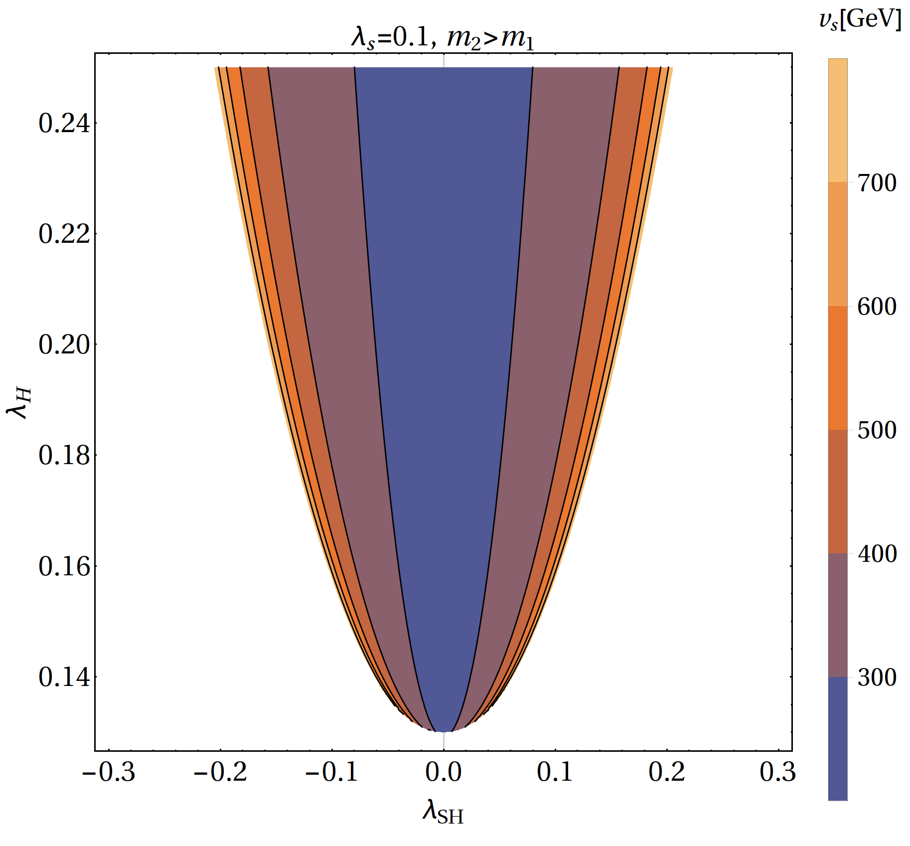
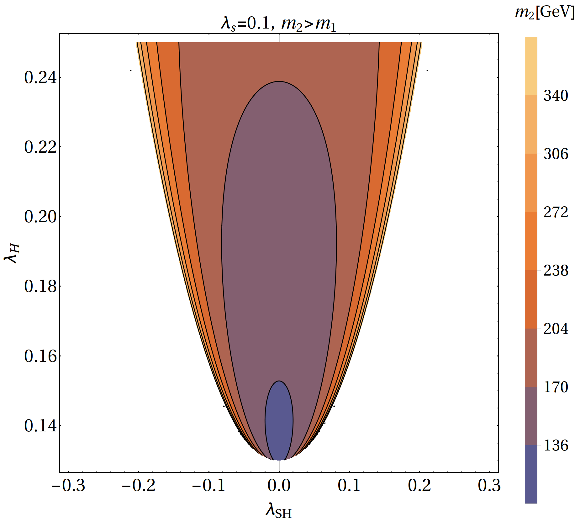
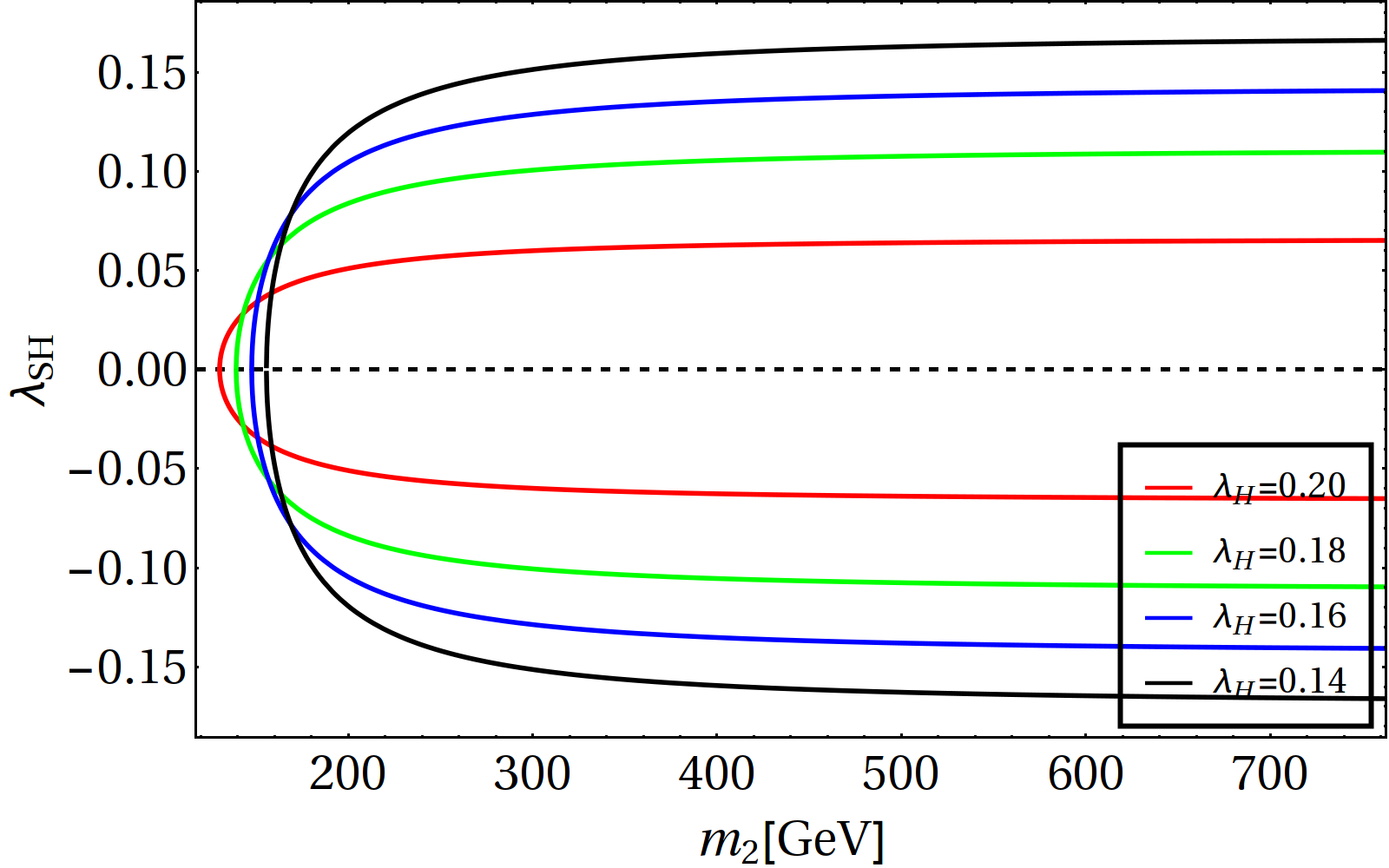
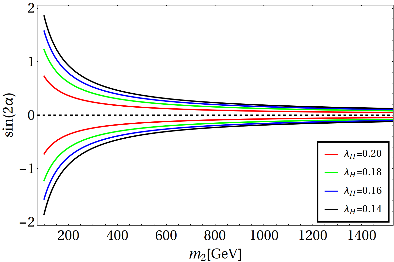
Figure 1: Top: The contours show allowed range of the vev $v_{S}$ and mass of the decoupled heavy scalar $m_{2}$ as a function of $\lambda_{H}$ and $\lambda_{SH}$ for fixed $\lambda_{S}=0.1$. Bottom left: $\lambda_{SH}$ as a functions of $m_{2}$ for fixed values of $\lambda_{H}$. Bottom right: $\sin(2\alpha)$ as a functions of $m_{2}$ for fixed values of $\lambda_{H}$. Decoupling of the dark sector is clearly seen in the limit of large $m_{2}$.

Now let’s define a current, $j_{\mu}\equiv(m_{X}X_{\mu}-\partial_{\mu}\sigma_{S})$. Then note that the following potentially relevant term, $j_{\mu}\partial^{\mu}\Phi$, is invariant under (2.4) and therefore could be added to the standard Stueckelberg Lagrangian. However, it turns out that this operator could be omitted. It has been shown in sec. 5 of ref. Duch:2014yma that terms $\propto j_{\mu}\partial^{\mu}\Phi$ could be removed from the Lagrangian by field redefinition: a shift of $B$ and rescaling of $\Phi$. Therefore hereafter $j_{\mu}\partial^{\mu}\Phi$ will be ignored. Alternatively one could also follow arguments of ref. Ruegg:2003ps , where the author argues that the operator $\propto j_{\mu}\partial^{\mu}\Phi$ does not contribute to the $S$-matrix elements between physical states.

Since our model is gauge invariant, the quantization requires fixing a gauge. We adopt the following gauge fixing term

$${\cal L}_{gf}=-\frac{1}{2\xi}\left(\partial^{\mu}X_{\mu}+\xi m_{X}\sigma_{S}\right)^{2}$$ (48)

The advantage of the adopted gauge fixing is that it cancels mixing between $\partial^{\mu}X_{\mu}$ and $\sigma_{S}$. Expanding the Lagrangian one obtains eventually

$${\cal L} = {\cal L}_{\text{lim}}+{\cal L}_{gf}=-\frac{1}{4}X_{\mu\nu}X^{\mu\nu}+\frac{m_{X}^{2}}{2}X_{\mu}X^{\mu}-\frac{1}{2\xi}\left(\partial^{\mu}X_{\mu}\right)^{2}+\frac{1}{2}\partial_{\mu}\sigma_{S}\partial^{\mu}\sigma_{S}-\frac{1}{2}\xi m_{X}^{2}\sigma_{S}^{2}+$$ (49)

$$+\frac{1}{2}\partial_{\mu}\Phi\partial^{\mu}\Phi+\frac{1}{2}\partial_{\mu}h\partial^{\mu}h-V_{\text{lim}}(h,\Phi)+\cdots\,.$$

In order to gauge-fix away $\sigma_{S}$ one must adopt the unitary gauge, which corresponds to $\xi\to\infty$. In the Stueckelberg formalism, in the unitary gauge, in presence of $\Phi$, one could expect presence of a term like $X_{\mu}X^{\mu}\Phi^{2}$ since it is allowed by symmetries. However, it turns out that the operator $X_{\mu}X^{\mu}\Phi^{2}$ may only originate from dimension-6 term $|D_{\mu}S|^{2}\Phi^{2}$ and therefore must be suppressed by $1/\Lambda^{2}$. This is the only gauge invariant way to generate an operator $\propto X_{\mu}X^{\mu}\Phi^{2}$. It explains why the operator $X_{\mu}X^{\mu}\Phi^{2}$ can not appear as an unsuppressed dimension-4 operator, even though naively it could be added within the Stueckelberg strategy.

The decoupling limit of the scalar potential consistent with all the theoretical constraints is illustrated in Fig. 1. In the top left panel, we show the allowed region in the $(\lambda_{H},\lambda_{SH})$ plane for $m_{2}>m_{1}$ where the colors varying from blue to yellow show larger $v_{s}$. Top right panel shows the same but coloring is with respect to $m_{2}$. Both these top panels show the decoupling limit at the outer edge of the allowed parameter space. In bottom left panel, we show $\lambda_{SH}$ as a function of $m_{2}$ at fixed values of $\lambda_{H}$. Similarly the bottom right figure shows $\sin(2\alpha)$ as a function of $m_{2}$, the convergence to zero-mixing angle is clearly shown.

Since the mixing angle vanishes in the limit $m_{2}\to\infty$, i.e. $\sin(2\alpha)\propto v_{h}/m_{2}$, therefore the dimension-4 interaction between dark vector and the SM disappears. Note also that since $\lambda_{S\Phi}$ could be negative, therefore for $\lambda_{S\Phi}<0$ one can always adjust $\mu_{\Phi}^{2}$ so that the $\Phi$ mass squared remains at the weak scale even if $v_{S}$ grows. On the other hand, for $\lambda_{S\Phi}>0$, to keep $m_{\Phi}$ at the weak scale $\lambda_{S\Phi}$ must behave as $\lambda_{S\Phi}\propto(v_{h}/v_{S})^{2}\propto(v_{h}/m_{2})^{2}$. In addition, since we want to retain the vector boson mass, $m_{X}=g_{X}v_{S}$, of the order of weak scale, therefore it is necessary that the gauge coupling diminishes as $g_{X}\propto(v_{h}/v_{S})^{2}\propto(v_{h}/m_{2})^{2}$. Note also that, since for large $m_{2}$ the value of the potential at the extremum # 4 diverges as $\sim-m_{2}^{4}/(16\lambda_{S})$ therefore in order to avoid instability while preserving perturbativity we must limit ourself to large, but finite, values of $m_{2}$.

Summarizing, to reach the Stueckelberg limit starting from the Lagrangian (3) a carefully adjusted trajectory in the parameter space must be adopted. An important consequence of approaching the $m_{2}\to\infty$ limit is the decoupling of the dark sector from the SM at dimension-4 operators by $\sin(2\alpha)\to 0$ and decoupling of $X_{\mu}$ from $S$ by $g_{X}\to 0$. It should also be recalled that to avoid instability of the potential $m_{2}$ must be finite (although can be large).

2.5 Higher dimensional operator to connect DM and SM sectors

Note that the coupling $\lambda_{H\Phi}$, which parametrizes the quartic portal interactions $\Phi^{2}|H|^{2}$, remains unsuppressed in the decoupling limit. Besides CP-violating operator $X_{\mu\nu}\tilde{X}^{\mu\nu}$  this is the only renormalizable (dim-4) communication between the dark and visible sectors in the limit. Leading corrections to this communication will be provided by dim-5 operators that are invariant under transformations from ${\cal G}=SU(3)_{C}\times SU(2)_{L}\times U(1)_{Y}\times U(1)_{X}\times Z_{2}$ and under Lorentz transformations and which are made of the scalar $\Phi$, the vector $X_{\mu}$ and possibly combinations of SM fields. It is easy to see that there are only two non-trivial operators that satisfy required symmetry conditions :

$${\cal L}_{\text{dim-5}}=\frac{c}{\Lambda}B_{\mu\nu}X^{\mu\nu}\Phi+\frac{\tilde{c}}{\Lambda}B_{\mu\nu}\tilde{X}^{\mu\nu}\Phi.$$ (50)

This operator has already been introduced in Macias:2015cna , where it was mentioned that such an operator can be generated at the tree level only via antisymmetric tensor mediators. Finally, one can then write down the complete Lagrangian as:

$${\cal L}_{\text{tot}} = {\cal L}_{\text{lim}}+{\cal L}_{gf}+{\cal L}_{\text{dim-5}}$$

$$= -\frac{1}{4}X_{\mu\nu}X^{\mu\nu}+\frac{m_{X}^{2}}{2}X_{\mu}X^{\mu}-\frac{1}{2\xi}\left(\partial^{\mu}X_{\mu}\right)^{2}+\frac{1}{2}\partial_{\mu}\sigma_{S}\partial^{\mu}\sigma_{S}-\frac{1}{2}\xi m_{X}^{2}\sigma_{S}^{2}+$$

$$+\frac{1}{2}\partial_{\mu}\Phi\partial^{\mu}\Phi+\frac{1}{2}\partial_{\mu}h\partial^{\mu}h-\left\{\frac{1}{2}m_{h}^{2}h^{2}+\lambda_{H}v_{h}h^{3}+\frac{1}{4}\lambda_{H}h^{4}+\right.$$

$$\left.+\frac{1}{2}m_{\Phi}^{2}\Phi^{2}+\lambda_{H\Phi}v_{h}h\Phi^{2}+\lambda_{\Phi}\Phi^{4}+\frac{1}{2}\lambda_{H\Phi}h^{2}\Phi^{2}+\text{const.}\right\}+\cdots+$$

$$+\frac{c}{\Lambda}B_{\mu\nu}X^{\mu\nu}\Phi+\frac{\tilde{c}}{\Lambda}B_{\mu\nu}\tilde{X}^{\mu\nu}\Phi\,,$$

where ellipsis denote interactions of the SM Higgs boson $h$ with other SM components that are not relevant here. We note here that we necessarily assume $\Lambda>m_{2}$, otherwise higher dimensional operators (neglected in this work) would appear in the scalar potential. We also adopt the following notations hereafter : $\alpha(\tilde{\alpha})=\frac{c(\tilde{c})}{\Lambda};~{}~{}\beta=\frac{\tilde{\alpha}}{\alpha}$.

3 DM yield via freeze-in

It is clear from the proceeding section that the couplings $\Phi\Phi h_{1}h_{1}$ and $\Phi\Phi h_{1}$ remain unsuppressed in the decoupling limit that we are exercising here. These interactions are $\propto\lambda_{H\Phi}$, which is not suppressed. This is the only renormalizable communication between the dark and visible sectors. So, it is quite likely to assume that in the early universe $\Phi$ is abundant being in equilibrium with the SM (i.e. with $h$). Since $\Phi$ is the next lightest $Z_{2}$-odd dark component its decays and annihilations may produce DM (i.e. $X$) non-thermally. This the mechanism (freeze-in) we will investigate hereafter. First, in this section, we will derive Boltzmann equations governing $X$ production in the early universe. We will also discuss applicability of neglecting various masses while calculating the amplitudes for decays and annihilations. Before going into the details, we would like to clarify that in the following sections, in order to satisfy the EFT limit and also have a successful freeze-in, we will adopt the following hierarchy amongst the scales and masses involved in the model:

$$\Lambda\mbox{\raisebox{-2.58334pt}{~{}$\stackrel{{\scriptstyle>}}{{\sim}}$~{}}}m_{2}\mbox{\raisebox{-2.58334pt}{~{}$\stackrel{{\scriptstyle>}}{{\sim}}$~{}}}T_{RH}>m_{\Phi}>m_{X},$$ (52)

where $T_{\text{RH}}$ is the reheating temperature at which inflaton decay products thermalize.

3.1 DM production via decay and annihilation processes

Since we are interested in the freeze-in production of the DM, hence we look for all such number changing processes with at least one DM particle in the final state. The processes that produce VDM, can easily be cooked up from interactions introduced in the preceding section and vertices collected in Appendix  B. We classify all the DM number changing processes on the basis of their occurrences before electroweak (EW) symmetry breaking (EWSB) i.e. for thermal bath temperature $T>T_{\text{EW}}\simeq 160~{}\rm GeV$ or after EWSB, i.e. for $T<T_{\text{EW}}$. Due to the presence of the $\Phi XB$ vertex the VDM $X$ can always be produced from the decay of the scalar $\Phi$ that maintains thermal equilibrium with the SM bath via the portal interaction $\lambda_{H\Phi}\left|H\right|^{2}\Phi^{2}$. This decay channel, shown in Fig. 2, is always present before and after EWSB as $m_{\Phi}>m_{X}$, which is anyway our prime assumption for the stability of the VDM. After EWSB, the decay occurs to $Z,\gamma$. Apart from the decay, we also have four $2\to 2$ annihilation channels with one DM in the final state as shown in Fig. 3 before EWSB . The processes include two t-channel and two s-channel graphs including Goldstone bosons ($\phi^{0,\pm}$). Note that, before EWSB all the SM states are massless and the Goldstone bosons (GB) are propagating degrees of freedom as the $SU(2)_{L}$ scalar has the form:

$$H=\begin{pmatrix}\phi^{+}\\ \phi^{0}\end{pmatrix}.$$ (53)

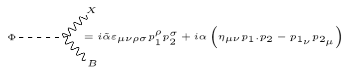
Figure 2: Decay of $\Phi\to XB$ before EWSB and $\Phi\to X\gamma(Z)$ after EWSB, which contributes to the freeze-in production of $X$. The vertex factor shown here is the one for $\Phi\to XB$.

The dark sector fields $\{\Phi,X\}$, on the other hand, are massive due to $U(1)_{X}$ breaking, which occurs at much higher energy scale. Due of the presence of totally anti-symmetric rank four Levi-Civita symbol in the interaction vertex $\Phi XB$ and the momenta dependent interaction vertices for the GB’s, all the processes involving Goldstone bosons in $t$-channel and $s$-channel identically become zero at the level of amplitude squared. Therefore, all those processes with GB’s drop out leaving only the $\Phi\to X,B$ decay channel, along with the two $2\to 2$ annihilation diagrams $f\Phi\to fX,~{}ff\to X\Phi$ (the top right and bottom left diagram of Fig. 3) for DM production via freeze-in before EWSB. However, as we shall see in subsequent sections, the decay before EWSB is sub-dominant as compared to the annihilation processes for large reheat temperature ($T_{\text{RH}}>>m$).

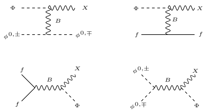
Figure 3: Annihilations via $t$-channel (top) and $s$-channel (bottom) leading to the production of VDM $X$ before EWSB. The diagrams with Goldstone bosons identically vanish, leaving only two diagrams with SM fermions.

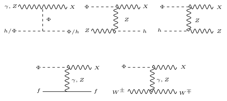
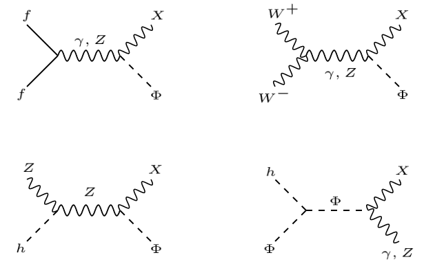
Figure 4: Annihilations via $t$-channel (left panel) and $s$-channel (right panel) leading to the production of $X$ after EWSB.

Once the EW symmetry is broken, the GB’s are no more individual physical degrees of freedom, instead they become longitudinal polarizations of the charged and neutral SM gauge bosons with $v_{h}=246~{}\rm GeV$. Also, the physical gauge bosons can be obtained in the mass basis by rotating the weak basis as:

$$\begin{pmatrix}B_{\mu}\\ W_{3\mu}\end{pmatrix}=\begin{pmatrix}c_{w}&-s_{w}\\ s_{w}&c_{w}\end{pmatrix}\begin{pmatrix}A_{\mu}\\ Z_{\mu}\end{pmatrix},$$ (54)

where $c(s)_{w}$ is the (co)sine of the Weinberg angle. Thus, after EWSB, the decay corresponds to $\Phi\to X,\gamma(Z)$, while all $2\to 2$ annihilation channels giving rise to DM final states are shown in Fig. 4. Due to massive propagator contributions after EWSB, the decay becomes more relevant for the determination of the DM yield, as we will demonstrate and discuss later. The decay widths and squares of the annihilation processes appearing before and after EWSB are collected in Appendix D.

3.2 Boltzmann equations for DM production

The key for freeze-in DM production is to assume that DM was not present in the early universe. In case it is produced via a decay as $\Phi\to BX$, the Boltzmann equation (BEQ) for the number density of $X$ can be written as:

$$\dot{n_{X}}+3Hn_{X}=\int d\Pi_{X}d\Pi_{B}d\Pi_{\Phi}\left(2\pi\right)^{4}\delta^{4}\left(p_{X}+p_{B}-p_{\Phi}\right)\left|\mathcal{M}\right|_{\text{D}}^{2}f_{\Phi},$$ (55)

where $d\Pi_{j}=\frac{d^{3}p_{j}}{2E_{j}\left(2\pi\right)^{3}}$ are Lorentz invariant phase space elements, and $f_{i}$ is the phase space density of the $i^{\text{th}}$ particle with corresponding number density being:

$$n_{i}=\frac{g_{i}}{\left(2\pi\right)^{3}}\int d^{3}pf_{i},$$ (56)

where $g_{i}$ is the number of internal DOFs. It is important to note that we assume negligible abundance of $X$ as the initial condition, also we disregard Pauli-blocking/stimulated emission effects, i.e. we assume $1\pm f_{i}\approx 1$. Indeed it has been assumed that $\Phi$’s are in equilibrium with the thermal bath (SM).

Similarly, the BEQ for DM production via generic annihilation process $i,j\to X,k$ (with one DM in the final state) reads Kolb:1990vq :

$$\dot{n_{X}}+3Hn_{X}=\sum_{i,j,k}\int d\Pi_{X}d\Pi_{i}d\Pi_{j}d\Pi_{k}\left(2\pi\right)^{4}\delta^{4}\left(p_{X}+p_{k}-p_{i}-p_{j}\right)\left|\mathcal{M}\right|_{i,j\to X,k}^{2}f_{i}f_{j}.$$ (57)

The BEQ in Eq. (57) can be rewritten as an integral over the CM energy as Edsjo:1997bg ; Hall:2009bx :

$$\dot{n_{X}}+3Hn_{X}\approx\frac{T}{512\pi^{6}}\sum_{i,j,k}\int_{0}^{\infty}dsd\Omega P_{ij}P_{Xk}\left|\mathcal{M}\right|_{i,j\to X,k}^{2}\frac{1}{\sqrt{s}}K_{1}\left(\frac{\sqrt{s}}{T}\right),$$ (58)

where $P_{ab}=\frac{1}{2\sqrt{s}}\sqrt{s-(m_{a}+m_{b})^{2}}\sqrt{s-(m_{a}-m_{b})^{2}}\to\frac{\sqrt{s}}{2}$ in the limit $m_{a,b}\to 0$.

Next we define the yield $Y_{X}\equiv n_{X}/s$, as a ratio of DM number density $n_{X}$ and the comoving entropy density in the visible sector $s$. The BEQ corresponding to the decay in terms of the yield $Y_{X}$ can be written in the differential form as:

$$\begin{split}-s(T)H(T)T\frac{dY_{X}^{\text{D}}}{dT}&=\frac{g_{\Phi}m_{\Phi}^{2}\Gamma_{\Phi\to X,B}}{2\pi^{2}}TK_{1}\left(m_{\Phi}/T\right),\end{split}$$ (59)

where we have defined:

$$\Gamma_{\Phi\to X,B}=\int\frac{1}{2m_{\Phi}}\frac{\left|\mathcal{M}\right|_{\Phi\to X,B}^{2}}{g_{\Phi}}\left(2\pi\right)^{4}\delta^{4}\left(p_{X}+p_{B}-p_{\Phi}\right)d\Pi_{X}d\Pi_{B}$$ (60)

as the decay width of $\Phi$. It is possible to express Eq. (59) in terms of the dimensionless quantity $x\equiv m_{X}/T$ and the reaction density $\gamma_{D}$ for decay as:

$$\begin{split}xHs\frac{dY_{X}^{\text{D}}}{dx}&=\gamma_{D},\end{split}$$ (61)

where $\gamma_{D}$, called reaction density, is defined in Appendix C.

For the case of annihilation one can similarly write:

$$\begin{split}-s(T)H(T)T\frac{dY_{X}^{\text{ann}}}{dT}&=\frac{T}{512\pi^{6}}\sum_{i,j,k}\int_{0}^{\infty}dsd\Omega P_{ij}P_{Xk}\left|\mathcal{M}\right|_{i,j\to X,k}^{2}\frac{1}{\sqrt{s}}K_{1}\left(\frac{\sqrt{s}}{T}\right).\end{split}$$ (62)

Note that the sum over $i,j,k$ indicates all the possibilities of producing DM following Figs. 3, and 4. Again, in terms of the reaction density defined in Appendix C, one can express the yield due to annihilation as:

$$\begin{split}xHs\frac{dY_{X}^{\text{ann}}}{dx}&=\gamma_{\text{ann}}.\end{split}$$ (63)

Following Eq. (59) and Eq. (62) the total yield due to decay and due to annihilation can be written as:

$$\begin{split}Y_{X}^{\text{total}}&=Y_{X}^{\text{D}}+Y_{X}^{\text{ann}},\\ &=\int_{T_{\text{min}}}^{T_{\text{max}}}dT\frac{m_{\Phi}^{2}\Gamma_{\Phi\to X,B}}{2\pi^{2}}\frac{K_{1}\left(m_{\Phi}/T\right)}{s(T)H(T)}\\ &+\frac{1}{512\pi^{6}}\sum_{i,j,k}\int_{T_{\text{min}}}^{T_{\text{max}}}\frac{dT}{s(T)H(T)}\int_{s=0}^{\infty}dsd\Omega\left(\frac{\sqrt{s}}{2}\right)^{2}\left|\mathcal{M}\right|_{i,j\to X,k}^{2}\frac{1}{\sqrt{s}}K_{1}\left(\frac{\sqrt{s}}{T}\right).\end{split}$$ (64)

The maximum temperature available to the process is what we call reheat temperature $T_{\text{RH}}$. Also, we note that the processes after EWSB, are different from those before. Therefore, taken all such processes together, the yield at temperature $T_{0}$ can finally be written as:

$$\begin{split}Y_{X}^{\text{total}}\left(T_{0}\right)&=\Bigg{\{}\int_{T_{\text{EW}}}^{T_{\text{RH}}}dT\frac{m_{\Phi}^{2}\Gamma_{\Phi\to X,B}}{2\pi^{2}}\frac{K_{1}\left(m_{\Phi}/T\right)}{s(T)H(T)}\\ &+\frac{1}{512\pi^{6}}\sum_{i,j,k}\int_{T_{\text{EW}}}^{T_{\text{RH}}}\frac{dT}{s(T)H(T)}\int_{0}^{\infty}dsd\Omega\left(\frac{\sqrt{s}}{2}\right)^{2}\left|\mathcal{M}^{\text{bEWSB}}\right|_{i,j\to X,k}^{2}\frac{1}{\sqrt{s}}K_{1}\left(\frac{\sqrt{s}}{T}\right)\Bigg{\}}\\ &+\Bigg{\{}\int_{T_{\text{0}}}^{T_{\text{EW}}}dT\frac{m_{\Phi}^{2}\Gamma_{\Phi\to X,\gamma(Z)}}{2\pi^{2}}\frac{K_{1}\left(m_{\Phi}/T\right)}{s(T)H(T)}\\ &+\frac{1}{512\pi^{6}}\sum_{i,j,k}\int_{T_{\text{0}}}^{T_{\text{EW}}}\frac{dT}{s(T)H(T)}\int_{0}^{\infty}dsd\Omega\left(\frac{\sqrt{s}}{2}\right)^{2}\left|\mathcal{M}^{\text{aEWSB}}\right|_{i,j\to X,k}^{2}\frac{1}{\sqrt{s}}K_{1}\left(\frac{\sqrt{s}}{T}\right)\Bigg{\}},\end{split}$$ (65)

where the first parenthesis corresponds to contribution before EWSB while the second one describes the after EWSB production and $\mathcal{M}^{\text{(a)bEWSB}}$ stands for the amplitude for processes appearing (after) before EWSB. Note that for the annihilation processes we have considered the massless approximation which makes the expression less complicated. One can, equivalently, express the BEQ in a more general manner in terms of the reaction densities utilising Eq. (61) and Eq. (63) as:

$$xHs\frac{dY_{X}}{dx}=\gamma_{\text{ann}}+\gamma_{\text{D}}.$$ (66)

This is rather more common and convenient way of parametrization. In Sec. 4 we will be using these reaction densities to compare DM yield before and after the EWSB.

3.3 UV limit and limitations

In this section, we demonstrate the difference between massless and massive limit of DM production cross-section and therefore we will be able comment on limitations of the Ultra Violet (UV) freeze-in advocated in Elahi:2014fsa ; Barman:2020plp . Here we limit ourself to the period before EWSB so all the SM particles are massless. The masses of the dark sector $\Phi$ and $X$ are assumed to be of the same order, typically $m_{\Phi}\sim m_{X}\sim m\sim{\cal O}(1\text{TeV})$. Hereafter the “massless limit” refers to zero-mass approximations, i.e. both SM and dark masses are zero. Our task in this section is to estimate size of mass effects, i.e. contributions to the yield that depend on the dark masses. Since we limit ourself to the temperatures above $T_{\text{EW}}$ therefore Eq. (65) can be simplified  as:

$$\begin{split}Y_{X}(T_{\text{EW}})&=\frac{1}{4\cdot 512\pi^{6}}\int_{T_{\text{EW}}}^{T_{\text{RH}}}\frac{dT}{s(T)\,H(T)}\\ &\int_{0}^{\infty}ds\left\{\int d\Omega\left|\mathcal{M}^{\text{bEWSB}}[s,\cos\theta]\right|_{i,j\to X,k}^{2}\right\}\sqrt{s}K_{1}\left(\frac{\sqrt{s}}{T}\right).\end{split}$$ (67)

Here onward we shall refer to $\mathcal{M}^{\text{bEWSB}}$ as $\mathcal{M}$.

For strictly massless case the integration over $s$ can be performed analytically, so the result reads

$$Y_{m=0}=AI(\theta_{min})\frac{45T_{RH}}{512\pi^{7}}\frac{16M_{pl}}{1.66g_{\star s}\sqrt{g_{\star\rho}}},$$ (68)

where $A$ contains all the couplings and constant factors that arise in the computation of $\left|\mathcal{M}^{m=0}[s,\cos\theta]\right|_{i,j\to X,k}^{2}$, and it is defined through the following relation:

$$\left|\mathcal{M}^{m=0}[s,\cos\theta]\right|_{i,j\to X,k}^{2}=Asm(\cos\theta),$$ (69)

with $m(\cos\theta)$ containing all the angular dependance of the amplitude squared while

$$I(\theta_{\text{min}})\equiv\frac{1}{2}\int_{-1}^{\cos\theta_{\text{min}}}d\cos\theta m(\cos\theta),$$ (70)

where $\theta_{\text{min}}$ is an angular cutoff necessary to avoid singularities that appear in the forward direction for t-channel diagrams, in the following $\theta_{\text{min}}=10^{-2}$ will be adopted.

  

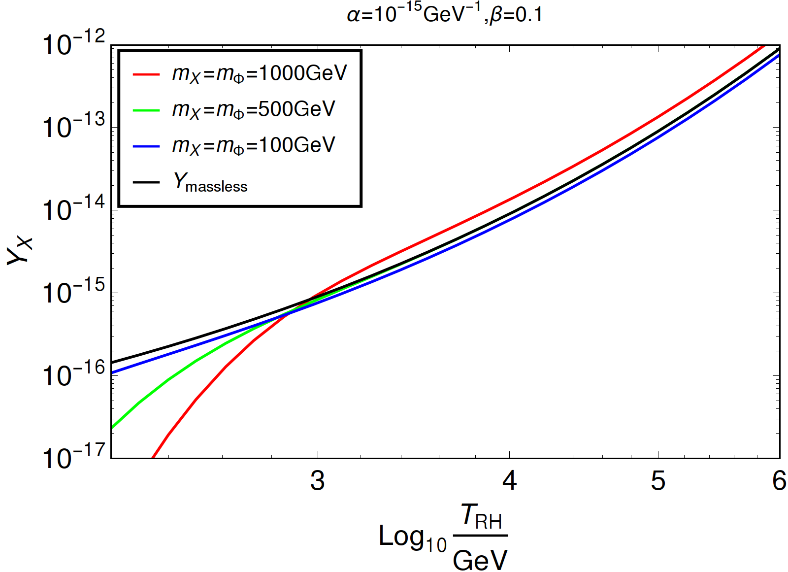
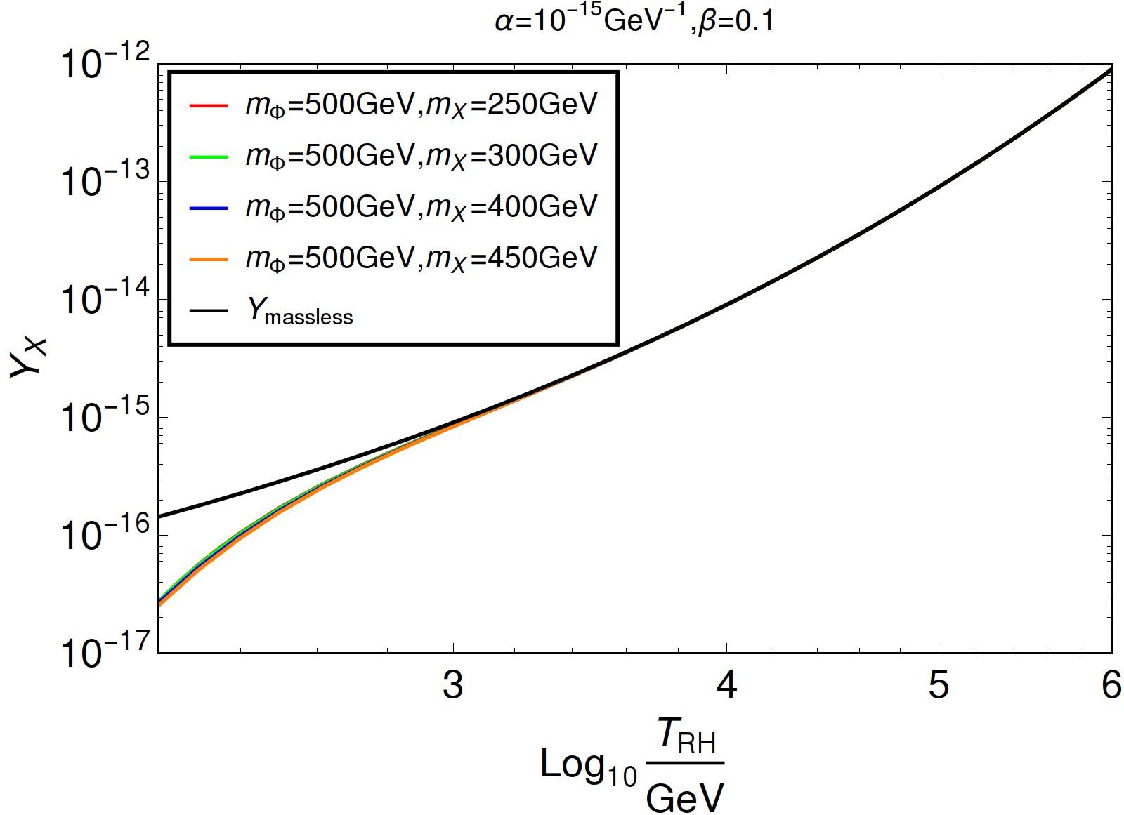
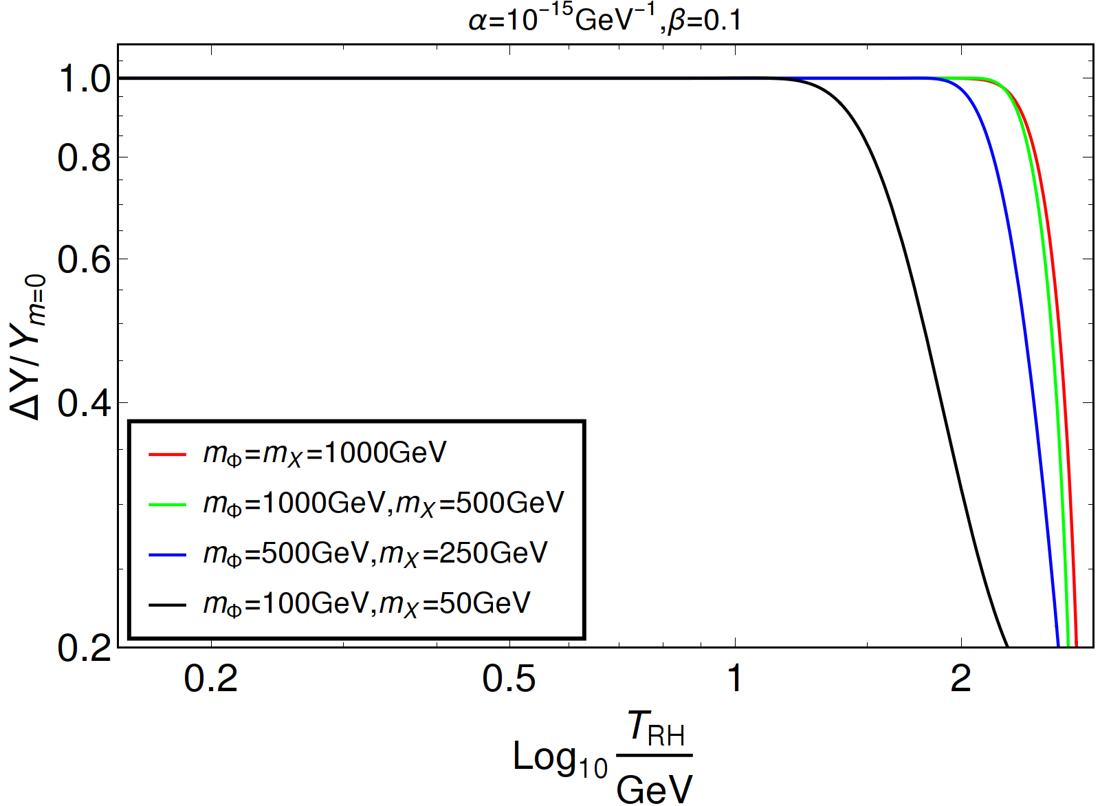
Figure 5: Top panels: Comparison of the yield at $T_{\text{EW}}$ in the massive case versus that in the massless case with respect to the reheat temperature, where the red, green and blue curves correspond to the massive cases while the black curve represents the massless case. Bottom panel: Variation of $\Delta Y/Y_{m=0}$ with the reheat temperature for different choices of the masses shown in different colors. In all the plots “massless” refers to $\to m=0$.

Now, we would like to estimate the difference between the massless and massive limit. For that, let us define:

$$\Delta Y(T)\equiv Y(T)|_{m=0}-Y(T)|_{m\neq 0}.$$ (71)

Also, note that,

$$\left|\mathcal{M}^{m\neq 0}[s,\cos\theta]\right|_{i,j\to X,k}^{2}=\left|\mathcal{M}^{m=0}[s,\cos\theta]\right|_{i,j\to X,k}^{2}+{\cal O}\left(\frac{m^{2}}{s}\right).$$ (72)

We assume here that the terms ${\cal O}\left(\frac{m^{2}}{s}\right)$ are negligible, note however that the mass dependance remains in $s_{\text{min}}=m^{2}$. Then, for processes with amplitude squared of the form given in Eq. (69) we find:

$$\Delta Y(T_{\text{EW}})\approx A\frac{45}{512\pi^{7}}\frac{I(\theta_{\text{min}})M_{\text{Pl}}}{1.66\cdot(g_{\star})^{1/2}g_{\star}^{s}}\int_{T_{\text{EW}}}^{T_{\text{RH}}}dT^{\prime}\;\int_{0}^{\frac{m}{T^{\prime}}}dx\,x^{4}K_{1}(x),$$ (73)

where $x\equiv\sqrt{s}/T$. As an example, let’s consider a $t$-channel process $\Phi f\to Xf$, where $f$ stands for the SM fermions. Then we find $I(\theta_{\text{min}})=1/2\int_{-1}^{\cos\theta_{\text{min}}}d\cos\theta(5+\cos\theta-\cos 2\theta)/(1-\cos\theta)\approx 75$. For $T_{\text{RH}}\gg m,T_{\text{EW}}$ we can estimate $\Delta Y(T_{\text{EW}})$ as follows

$$\Delta Y(T_{\text{EW}}) \approx AI(\theta_{min})\frac{45}{512\pi^{7}}\frac{M_{pl}}{1.66g_{\star s}\sqrt{g_{\star\rho}}}4.65m.$$ (74)

Note that $\Delta Y(T_{\text{EW}})$ is linear in $m$ as it obviously should vanish in the limit $m\to 0$. We should also note that Eq. (74) is process independent and can be written in this particular form whenever the matrix element squared can be expressed in the form of Eq. (69).

Now, let us find out the condition under which $\Delta Y$ becomes as large as $Y_{\text{massless}}$, as that will dictate the condition for which massless limit can be no longer adopted for the UV freeze-in scenario. This can simply be found out by equating Eq. (74) and Eq. (68):

$$\begin{split}\Delta Y&=AI(\theta_{min})\frac{45}{512\pi^{7}}\frac{M_{pl}}{1.66g_{\star s}\sqrt{g_{\star\rho}}}\Biggl{(}m\int_{0}^{T_{\text{RH}}/m}dug(u)\Biggr{)}\mbox{\raisebox{-2.58334pt}{~{}$\stackrel{{\scriptstyle<}}{{\sim}}$~{}}}Y_{m=0}\\ &\implies m\mbox{\raisebox{-2.58334pt}{~{}$\stackrel{{\scriptstyle<}}{{\sim}}$~{}}}3.5~{}T_{\text{RH}}.\end{split}$$ (75)

This implies that, as long as the masses involved in the freeze-in process are approximately less that three times of the reheat temperature, one can overlook the masses and the yield can be computed in the massless limit. This, in other words, justifies the fact that for large reheat temperature the massless limit is a good approximation for obtaining the UV freeze-in yield. In Fig. 5, we demonstrate the difference between the yield obtained for massive and massless case of DM production for all the processes before EWSB put together. We plot $Y_{X}(T=T_{EW})$ as a function of $T_{\text{RH}}$ and see that massive case sharply differs from the massless case (black line) at small $T_{\text{RH}}$, while they exactly merge as the reheat temperature becomes large. In the bottom panel we show the same feature in terms of $\frac{\Delta Y}{Y_{m=0}}$ for different choices of $m_{X,\Phi}$.

4 DM relic abundance via freeze-in

As described in details in the last section, within the freeze-in paradigm, the DM yield is controlled by the annihilation and/or decay of SM as well as dark sector particles. Following Eq. (66) we write down the BEQ governing the DM yield as Duch:2017khv :

$$xHs\frac{dY_{X}}{dx}=\gamma_{\text{ann}}+\gamma_{\text{D}},$$ (76)

where $Y_{X}=n_{X}/s$. $H$ is the Hubble parameter given by $H=1.66\sqrt{g_{\star\rho}}T^{2}/M_{pl}$ and $x=m_{X}/T$ is a dimensionless quantity to parametrize the temperature of the thermal bath. As mentioned earlier, the $\gamma$’s denote the so-called reaction density for different particles annihilating (decaying) to the DM. The detail expressions of the reaction densities for $2\to 2$ annihilations and $1\to 2$ decays are given in Appendix. C. In order to compute the DM yield, we solve Eq. (76) with the initial condition $Y_{X}\approx 0$ at large $T$ i.e., small $x$ in accordance with the usual FIMP set-up . By solving Eq. (76) one can obtain the total DM yield $Y_{X}$ at the present epoch i.e., $Y_{X}(T_{0})$. The relic abundance of $X$ at present temperature can then be obtained via:

$$\Omega_{X}h^{2}=\left(2.75\times 10^{8}\right)\left(\frac{m_{X}}{\text{GeV}}\right)Y_{X}(T_{0}).$$ (77)

We must also remind that the PLANCK Aghanim:2018eyx allowed relic density reads:

$$\Omega h^{2}=0.11933\pm 0.00091,$$ (78)

which we will use to find the relic density allowed parameter space of the model.

Since in our case the connection between the dark and the visible sector proceeds via a non-renormalizable interaction, the DM abundance is usually characterized by UV freeze-in Elahi:2014fsa ; Barman:2020plp limit, where the DM abundance is sensitive to the reheat temperature $T_{\text{RH}}$ of the universe and NP scale $\Lambda$ only. This is in sharp contrast to the Infra-Red or IR freeze-in scenario where the two sectors communicate via renormalizable operators, and the DM abundance is set by the IR physics i.e., the yield becomes maximum at low temperature, typically at $T\sim m_{X}$ Hall:2009bx . Now, the reheat temperature $T_{\text{RH}}$ is very loosely bounded. Typically, the lower bound on $T_{\text{RH}}$ comes from the measurement of light element abundance during Big Bang Nucleosynthesis (BBN), which requires $T_{\text{RH}}\gtrsim 4.7~{}\rm MeV$ deSalas:2015glj . The upper bound, on the other hand, comes from (a) cosmological gravitino problem Moroi:1993mb ; Kawasaki:1994af in the context of supersymmetry, that demands $T_{\text{RH}}\lesssim 10^{10}~{}\rm GeV$ to prohibit gravitino over production and (b) simple inflationary scenarios that require $T_{\text{RH}}\sim 10^{16}~{}\rm GeV$ Kofman:1997yn ; Linde:2005ht for a successful inflation. The reheat temperature, thus, can be regarded as a free parameter for our analysis. As we have already shown in the preceding section, when reheat temperature drops close to the masses involved in the annihilation or DM production process, massive kinematics start playing a key role in the yield and UV limit can not be trusted. Therefore our analysis will be divided into two regimes, depending on the scale of the reheat temperature $(T_{\text{RH}})$:

• $T_{\text{RH}}>>m_{i}$, where the reheat temperature lies way above different masses that appear in the model.

• $T_{\text{RH}}\gtrsim m_{i}$, where the reheat temperature lies close to the masses in the theory.

In the following sub-sections we will consider the above two cases. It is important to point out that our calculations of cross-sections have all been done analytically (see Appendices) and then the relic density is found out by solving BEQ in Mathematica numerically.

4.1 Large reheat temperature: $T_{\text{RH}}>>m$

In this sub-section the reheat temperature is assumed to be much larger than the dark sector masses. We would like to mention that computing the reaction densities, we consider both $2\to 2$ annihilation channels and $\Phi\to XB$ decay channel before EWSB, while after EWSB we only take into account the $\Phi\to XZ(\gamma)$ decays for reasons elaborated soon. Also note that, all the SM fields are massless before EWSB but the dark sector fields ($m_{\Phi},m_{X}$) are massive irrespective of the era, thanks to $U(1)_{X}$ breaking at very high scale. First we compare reactions densities for annihilation and the decay as a function of $x\equiv m_{X}/T$. Often we use a dimensionless variable $r=\frac{m_{X}}{m_{\Phi}}<1$ to illustrate scan results.

  

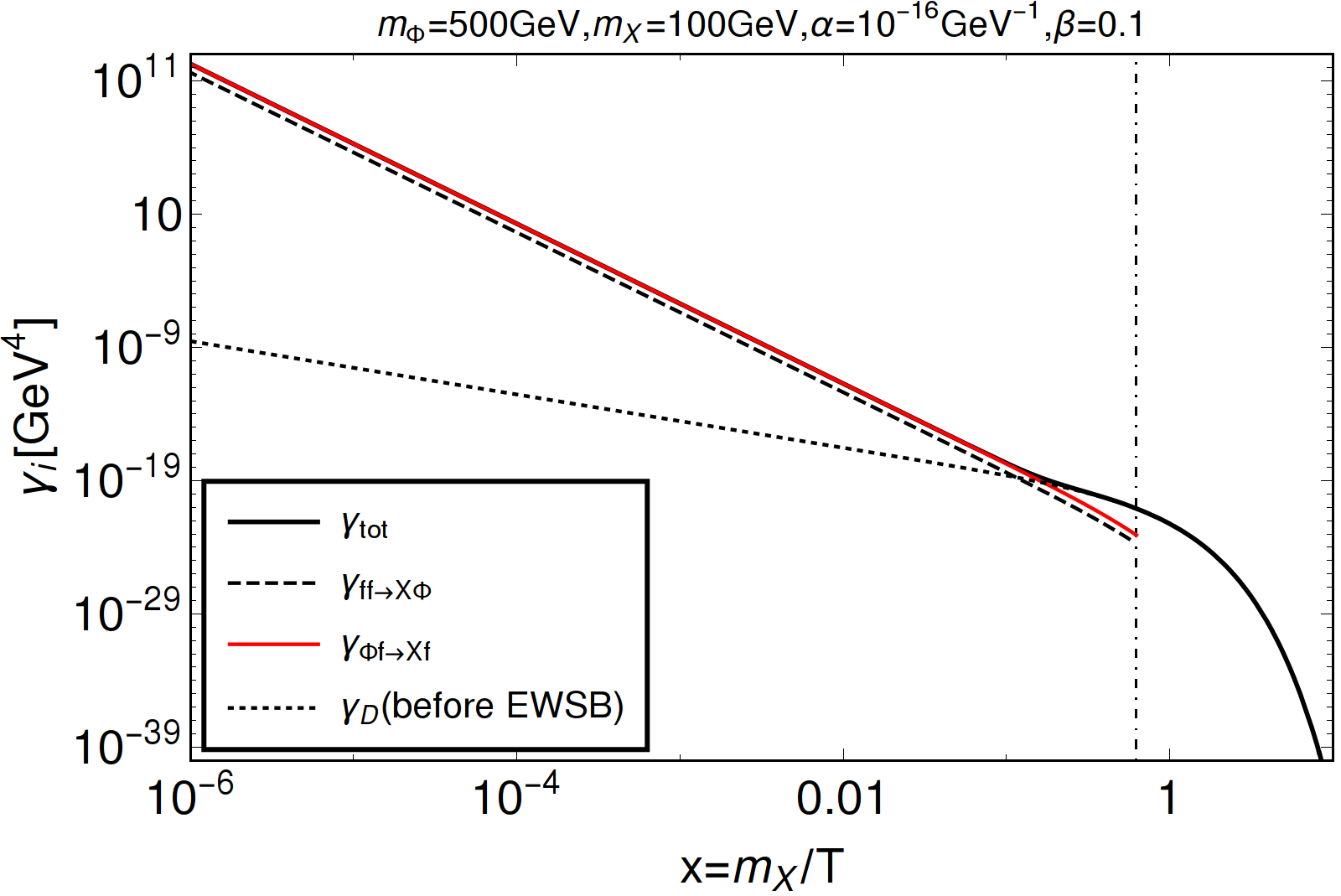
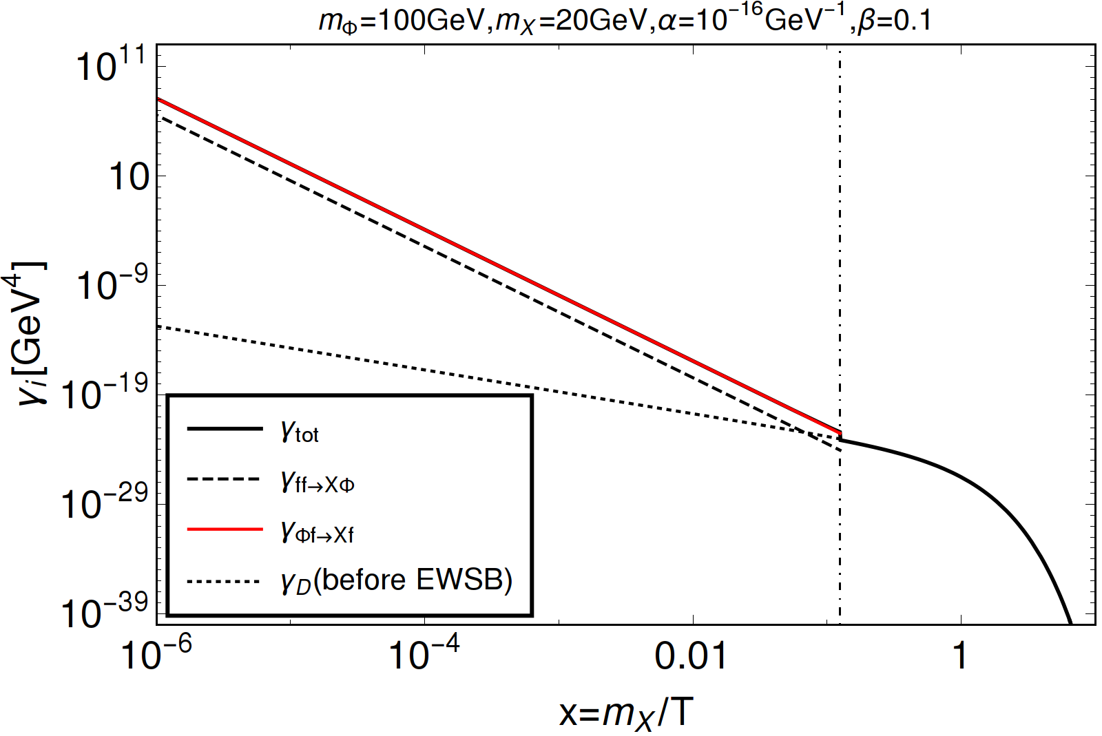
Figure 6: Comparison of reaction densities ($\gamma_{\text{ann,D}}$) for annihilation and the decay. Before EWSB we show the $s$-channel $\bar{f}f\to X\Phi$ process (black dashed) and $t$-channel $\Phi f\to Xf$ (red) and also the decay contribution (black doted), while after EWSB we plot the density for the decay (solid black) only. The solid black line (hidden beneath the red line before EWSB) shows both contributions from the annihilation and the decay together. In the left panel we choose $m_{\Phi}=500~{}\text{GeV},~{}m_{X}=100~{}\text{GeV}$, while in the right, we choose $m_{\Phi}=100~{}\text{GeV},~{}m_{X}=20~{}\text{GeV}$. In both cases we have $\alpha=10^{-16}~{}\text{GeV}^{-1},\beta=0.1$. The vertical dashed-dotted lines shows $x$ corresponding to EWSB.

In Fig. 6 we show individual contributions of annihilations and the decay to the reaction densities as a function of $x$ keeping the DM mass, the $\Phi$ mass, and the coupling $\alpha(\tilde{\alpha})$ fixed. The vertical dashed-dotted line represents EWSB $x_{EW}=m_{X}/T_{EW}$. Here we clearly see that the reaction densities due to the $s$-channel and $t$-channel annihilation processes are much larger than that due to decay before EWSB, while after EWSB the reaction density falls to a very small value.

The suppression of the decay before EWSB can be understood comparing the analytical forms of reaction densities for annihilation (in massless limit) and decay as follows:

$$q\equiv\frac{\gamma_{\text{ann}}}{\gamma_{\text{D}}}\sim\frac{\int_{0}^{\infty}dss^{3/2}\sigma_{ann}(s)K_{1}\left(\sqrt{s}/T\right)}{\alpha^{2}(1+\beta^{2})m_{\Phi}^{5}K_{1}\left(m_{\Phi}/T\right)}\sim\left(\frac{T}{m_{\Phi}}\right)^{5}\frac{1}{K_{1}\left(m_{\Phi}/T\right)},$$ (79)

where $\sigma_{ann}(s)\propto\alpha^{2}(1+\beta^{2})\times\text{const.}$ was assumed. It then follows that for $T>>m_{\Phi}\implies q\gg 1$ and for $T\sim m_{\Phi}\implies q\sim 1$. We however, would like to caution the reader that above formula is not strictly valid at $T$ close to EWSB when massive kinematics become important for computing annihilation cross-sections as elaborated in Sec. 3.3.

This implies that the DM is dominantly produced before EWSB, while the yield accumulated after EWSB is negligibly small. This is a typical feature of UV freeze-in where the maximum yield production happens at high temperature. An evolution of the total reaction density taking into account all annihilation processes occurring before EWSB together with the decay after EWSB for different sets of $\{m_{\Phi},m_{X}\}$ is shown in Fig. 7. It is clear from the discussion above that decay contribution before EWSB is very small, while the contribution from decay is dominant over annihilation processes after EWSB. Note here that the vertical dashed-dotted lines in different colors represent EWSB at $x_{EW}=m_{X}/T_{EW}$ corresponding to those $m_{X}$ values chosen for illustration.

  

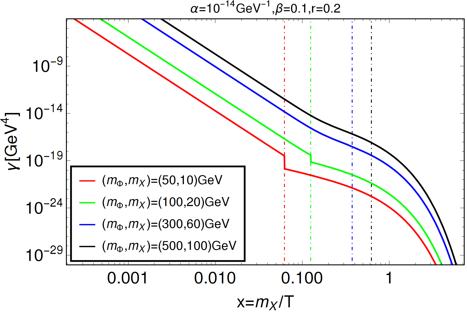
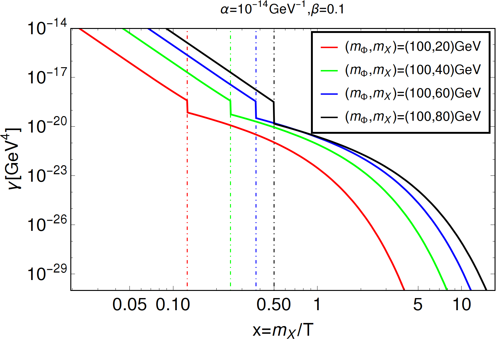
Figure 7: Total reaction density over the whole range of temperature before and after EWSB taking into account both annihilation and decay before EWSB, but only decay after EWSB. We consider all SM states to be massless before EWSB, while dark sector particles are massive. The dashed-dotted vertical lines correspond to $x_{EW}=\frac{m_{X}}{T_{EW}}$ for each choice of DM mass. In the left panel we show densities for different choices of $m_{\Phi}=\{50,100,300,500\}~{}\rm GeV$ (in red, green, blue, black, respectively) for fixed $r=\frac{m_{X}}{m_{\Phi}}=0.2$, while in the right one they are shown for different $r=\{0.2,0.4,0.6,0.8\}$ (in red, green, blue, black, respectively) for fixed $m_{\Phi}=100~{}\rm GeV$. In both cases we choose $\alpha=10^{-14}~{}\text{GeV}^{-1},\beta=0.1$.

Also note that for $m_{\Phi}\lesssim 100~{}\rm GeV$, the reaction densities in two regimes before and after EWSB can be distinctively identified by a step, while that for larger $m_{\Phi}$ they are continuous. This is because with temperature dropping, the $2\to 2$ production cross-sections drops and around $T_{EW}$ the decay contribution dominates over them, resulting a continuous curve before and after EWSB. However, after EWSB, the decay final state changes from $\Phi\to X,B$ to $\Phi\to X,\gamma(Z)$. Therefore when $m_{\Phi}<m_{X}+m_{Z}$, one of the decay processes, $\Phi\to X,Z$, become kinematically forbidden showing a distinct drop in the reaction density. The values of different parameters chosen for illustration are mentioned in figure inset.

  

  

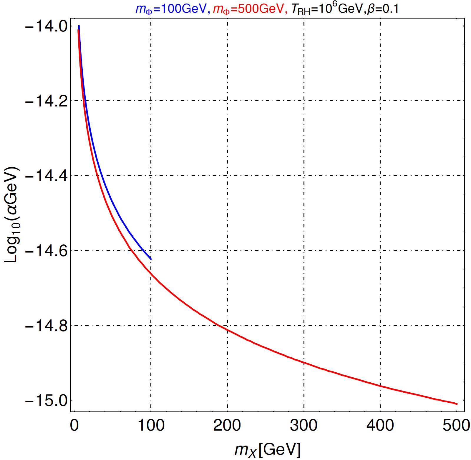
Figure 8: Top left: evolution of the DM yield $Y_{X}$ for parameters which imply correct relic DM abundance as a function of $x=m_{X}/T$ obtained by solving Eq. (76). Here different colored curves indicate different choices of $r=\frac{m_{X}}{m_{\Phi}}=\{0.1,0.2,0.4,0.6\}$ in red, green, blue and black respectively for a fixed $m_{\Phi}=100~{}\text{GeV},\alpha=10^{-16}~{}\text{GeV}^{-1},\beta=0.1$ and reheat temperature $T_{\text{RH}}=10^{8}~{}\rm GeV$. The vertical dashed-dotted lines correspond to $x_{\text{EW}}=m_{X}/T_{\text{EW}}$ for different values of $m_{X}$. Top right: same as top left but with $m_{\Phi}=500~{}\rm GeV$. Bottom left: relic density allowed parameter space in terms of $m_{X}-\alpha$ where different colored contours correspond to $m_{\Phi}=500~{}\rm GeV$ (red) and $m_{\Phi}=100~{}\rm GeV$ (blue) for a fixed $\beta=\frac{\tilde{\alpha}}{\alpha}=0.1$ and reheat temperature $T_{\text{RH}}=10^{8}~{}\rm GeV$. Bottom right: same as bottom left but with $T_{\text{RH}}=10^{6}~{}\rm GeV$.

The effect of large reheat temperature and large reaction densities at high temperature is reflected in the DM yield shown in the top panels of Fig. 8. In both scans we keep $T_{RH}=10^{8}$ GeV. In the top panel of Fig. 8 we see that the DM yield builds up quickly with $x$ (i.e. with lowering temperature) and reaches its maximal value already at very high temperature $T\sim T_{\text{RH}}$. Then it freezes-in immediately producing an yield that remains constant till $T=T_{0}\simeq 2.73~{}\rm K$. The asymptotic value of the yield, $Y_{0}\equiv Y(T_{0})$, directly implies the PLANCK observed DM relic abundance via (77). As seen from (77) each choice of the DM mass requires appropriate $Y_{0}$ what results in the splitting of the colored curves at large $x$ observed in Fig. 8. On the other hand each $Y_{0}$ requires the couplings $\alpha,\tilde{\alpha}$ tuned appropriately, as shown in the legend of Fig. 8. The left top panel corresponds to $m_{\Phi}=500$ GeV, while the top right panel to slightly smaller value $m_{\Phi}=100$ GeV. The vertical dashed lines show the locations of EWSB, although its effect on the final yield is invisible. In the bottom panels of Fig. 8 we show contours corresponding to the central value of the PLANCK observed relic abundance ($\Omega h^{2}\simeq 0.1199$) in the $\alpha-m_{X}$ plane for fixed $m_{\Phi}=500\;\text{GeV}$ and $100\;\text{GeV}$ and two different values of $T_{\text{RH}}$. The left and right lower panels correspond to the reheat temperature $T_{\text{RH}}=10^{8}$ and $10^{6}\;\text{GeV}$, respectively. The relic abundance is obtained following Eq. (77). Since $\Omega_{X}\propto m_{X}$, we see for larger DM mass smaller $\alpha$ is required to compensate for the over abundance. Note, that in each panel the kinematical condition $m_{\Phi}\gtrsim m_{X}$ is obeyed. As expected, for the same DM mass, growing $T_{\text{RH}}$ requires lower couplings. We would finally note that to find yield in such a scenario, the masses in all reactions can be safely neglected and the processes after EWSB contributes negligibly.

DM production via annihilation or decay processes can also be compared (at $T_{0}\sim 0\;\text{GeV}$) by naive dimensional analysis as advocated in Hall:2009bx ; Cheung:2010gj :

$$\frac{Y_{X}^{ann}}{Y_{X}^{\text{D}}}\sim\frac{\sigma M_{pl}T_{FI}}{\Gamma_{\Phi}M_{pl}/T_{FI}^{2}}\sim\frac{\alpha^{2}M_{pl}T_{RH}}{\left(\alpha^{2}m_{\Phi}^{3}\right)M_{pl}/m_{\Phi}^{2}}\sim\frac{T_{RH}}{m_{\Phi}},$$ (80)

where $T_{FI}$ denotes the characteristic freeze-in temperature scale at which the yield reaches the constant value (see e.g the plateau in upper panels of Fig. 8) for DM production via annihilation process or decay, which are not quite the same. For decays, the freeze-in temperature can be assumed to be the mass of the decaying particle, i.e. $T_{FI}\sim m_{\Phi}$, which is used in the second step of the above analysis. On the other hand, for DM yield produced via annihilation process, the freeze-in temperature can be assumed to be the highest temperature available for the process, i.e. $T_{FI}\sim T_{RH}$. Therefore, for $T_{RH}>>m_{\Phi}$ ensures that annihilation contribution dominates over decay contribution in the final yield for UV limit. This brings us to an asymptotic formula of the yield in UV limit, which can simply be written as:

$$Y_{X}(x=0)\sim\alpha^{2}M_{pl}T_{RH},$$ (81)

neglecting the decay contribution and is validated in Fig. 11, as we explain in a moment.

4.2 Low reheat temperature: $T_{\text{RH}}\gtrsim m$

This case is more interesting. It turns out that when the reheat temperature drops down to $\sim\text{TeV}$ scale, then processes that take place after EWSB are relevant and contribute significantly to final yield. After EWSB all the SM states also become massive, and hence in order to get meaningful results, all masses shall be kept. As we shall see, in such a case the IR freeze-in starts showing up, i.e. the freeze-in takes place at a temperature $T\sim m_{X}$.

  

  

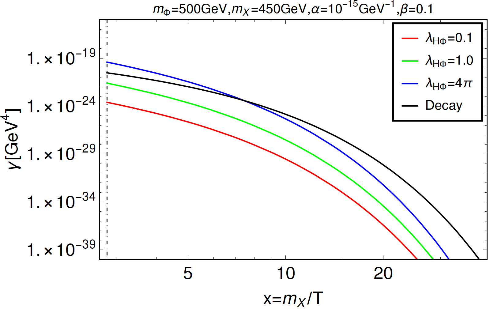
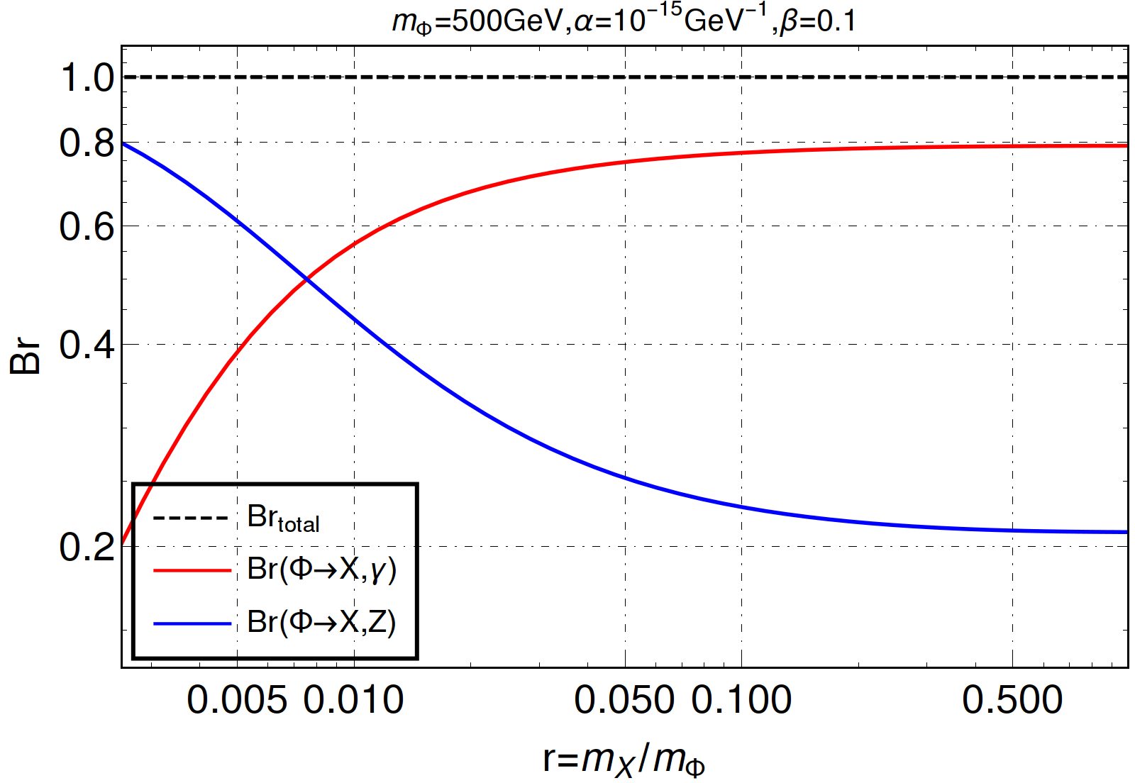
Figure 9: Top panel: Comparison of reaction densities due to annihilation (colorful lines) and decay (shown in black) after EWSB. Contributions of two annihilation channels are shown: $h,\Phi\to X,Z$ via $Z$ boson mediation in $t$-channel and $h,\Phi\to X,\gamma(Z)$ via $\Phi$ mediation in $s$-channel. All states are assumed to be massive. The amplitudes for $h,\Phi\to X,\gamma(Z)$ channel are proportional to the portal coupling $\lambda_{H\Phi}$ that is being varied in the plots. The choice of parameters is specified in the headings. Bottom panel: Decay branching fraction of $\Phi\to X\gamma(Z)$ as function of $r=\frac{m_{X}}{m_{\Phi}}$.

    

  

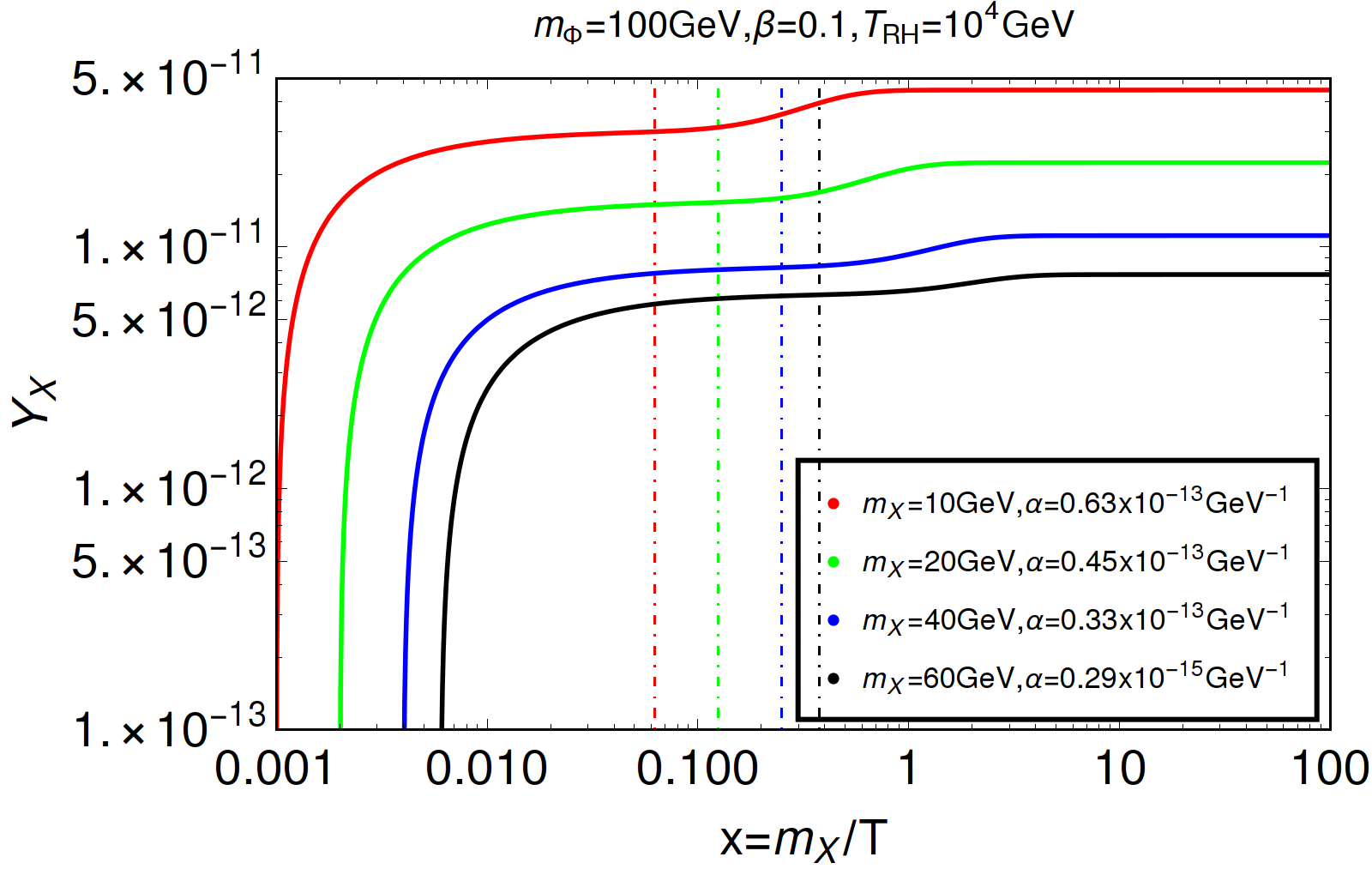
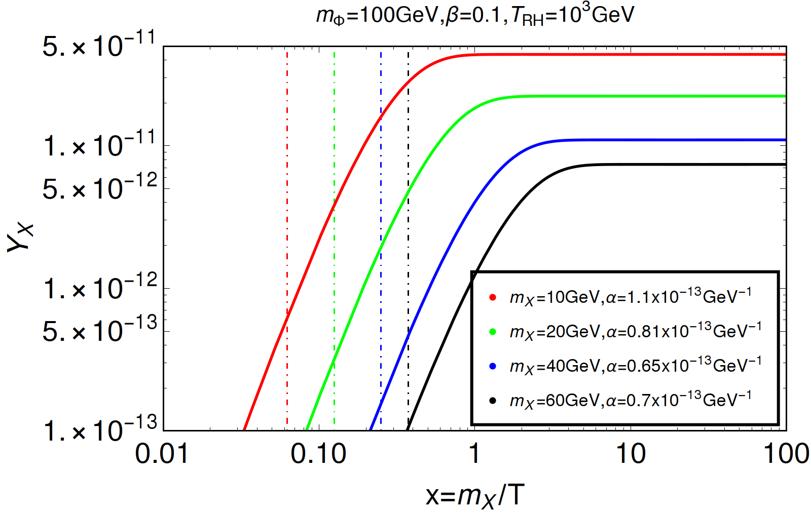
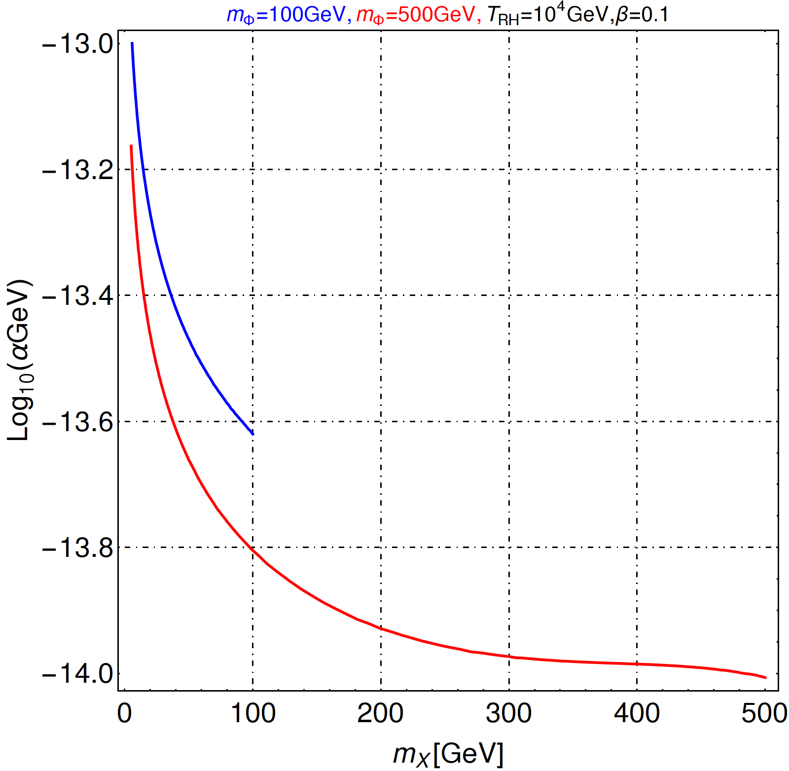
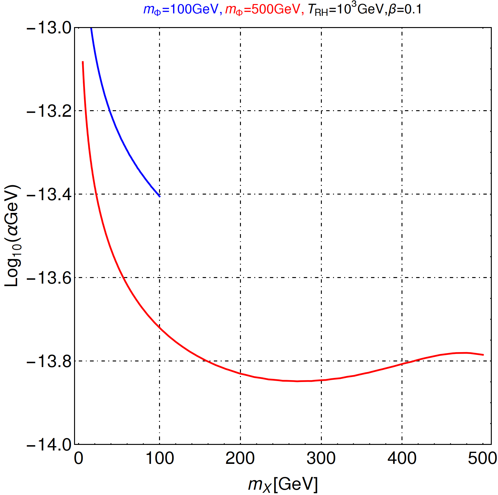
Figure 10: Top left: DM yield as a function of $x=m_{X}/T$ for a reheat temperature $T_{\text{RH}}=10\;\text{TeV}$ considering both annihilation and decay to be active before EWSB, while keeping only decay after EWSB. We choose $m_{\Phi}=100\;\text{GeV}$ and $\beta=0.1$ while for each value of $m_{X}$, $\alpha$ is adjusted to reproduce the central value of the measured relic abundance. Top right: Same as top left but with $T_{\text{RH}}=1\;\text{TeV}$. In both of the plots the vertical dashed lines denote EWSB ($x_{EW}$). Bottom left: Relic density allowed parameter space in $m_{X}-\alpha$ plane for $T_{\text{RH}}=10\;\text{TeV}$ and $\alpha$ adjusted to reproduce the DM abundance. Bottom right: Same as bottom left but with $T_{\text{RH}}=1~{}\rm TeV$.

Before solving BEQ, let us estimate first the hierarchy of reaction densities. For illustration, in Fig. 9, we compare reaction densities for the $\Phi$ decay and those for annihilations into $X,\gamma(Z)$ final states. For the later final state two annihilation diagrams contribute: (a) $t$-channel annihilation $h,\Phi\to X,Z$ via $Z$ boson mediation and (b) $s$-channel process $h,\Phi\to X,\gamma(Z)$ via $\Phi$ mediation. We consider all the states involved in these two processes to be massive. Note that the s-channel amplitude for $h,\Phi\to X,\gamma(Z)$ is proportional to $\lambda_{H\Phi}$, therefore it could be amplified. We show the reaction density as a function of $x$ for decay as the black curve in all the figures, while we choose three values of $\lambda_{H\Phi}=\{0.1,1,4\pi\}$, shown respectively in red, green and blue, for the annihilation processes. It is seen that for small $m_{X}\simeq 100~{}\rm GeV$, after EWSB the decay dominates over annihilation even when the portal coupling is close to its limiting perturbative value i.e. $4\pi$. However for $m_{X}\gtrsim 400~{}\rm GeV$ and $\lambda_{H\Phi}\simeq 4\pi$ the $s$-channel annihilation starts dominating over decay for $x\mbox{\raisebox{-2.58334pt}{~{}$\stackrel{{\scriptstyle<}}{{\sim}}$~{}}}7$. This is expected since growing DM mass causes phase space suppression of the decay width. However, even for $m_{X}\simeq 499\;\text{GeV}$ for large enough $x$ again the decay dominates over annihilation. Therefore, it is fair to conclude that as long as $\lambda_{H\Phi}\lesssim\mathcal{O}(1)$, one can safely ignore all the annihilation processes even for large DM mass. In the bottom panel of Fig. 9 we show variation of $\Phi$-branching ratio to $X$ and photon or $Z$-boson. For light $X$, $\Phi$ decays into $X,Z$ dominate while for $r=m_{X}/m_{\Phi}\mbox{\raisebox{-2.58334pt}{~{}$\stackrel{{\scriptstyle>}}{{\sim}}$~{}}}0.008$ $\Phi$ decays mostly into $X\gamma$.

  

   

   

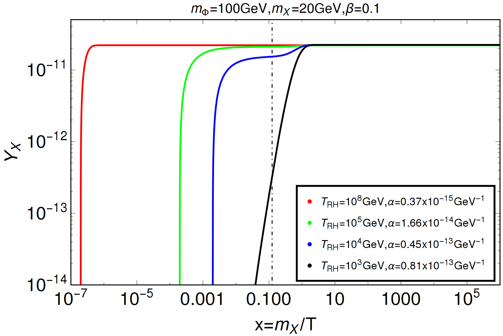
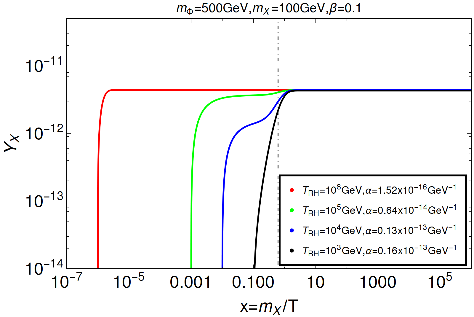
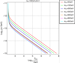
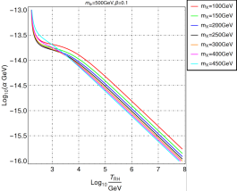
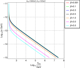
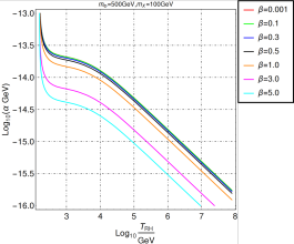
Figure 11: Top panel: DM yield as a function of temperature for different choices of the reheat temperature $T_{\text{RH}}:\{10^{5},10^{2},10,1\}~{}\rm TeV$ shown in red, green, blue and black curves respectively. Here we have considered both annihilation and decay channels before EWSB where SM particles are massless while the dark particles are massive. In the post-EWSB scenario we have considered only the decays with massive states. The parameters chosen correspond to right relic abundance. In each of these plots the vertical dashed-dotted lines denote EWSB ($x_{EW}$). Middle left: Relic density allowed parameter space in terms of $\alpha-T_{\text{RH}}$ where different colored contours correspond to different $m_{X}$ for a fixed $m_{\Phi}=100~{}\rm GeV$. Middle right: Same as middle left panel, but for a different fixed $m_{\Phi}=500~{}\rm GeV$. Bottom left: Same as middle panel but for different choices of $\beta:\{0.001,0.1,0.3,0.5,1.0,3.0,5.0\}$ for $m_{\Phi}=100~{}\text{GeV}$ and $m_{X}=10~{}\text{GeV}$. Bottom right: Same as bottom left with $m_{\Phi}=500~{}\text{GeV}$ and $m_{X}=100~{}\text{GeV}$

Now let us find relic density in the low $T_{\text{RH}}$ regime. In the left and right upper panels of Fig. 10 we have shown the DM yield for several values of $m_{X}$ as a function of $x$ for $T_{\text{RH}}=10^{4}\;\text{GeV}$ and $10^{3}\;\text{GeV}$, respectively. In order to satisfy the relic abundance, for smaller $T_{\text{RH}}$, we need larger $\alpha$ as $Y_{X}\sim T_{\text{RH}}\alpha^{2}$. Note that the left panel already shows formation of IR-like behavior of the yield that is typical for low $T_{\text{RH}}$: the “second slopes” that appear for larger $x$ in the left panel ($T_{\text{RH}}=10^{4}\;\text{GeV}$) reach their corresponding plateaus at the same location as in the right panel for $T_{\text{RH}}=10^{3}\;\text{GeV}$. In the right panel, the typical UV-like sudden DM production disappeared leaving only after-EWSB IR-production (decays) at much larger $x$. The IR behavior is, of course, more prominent for smaller $T_{\text{RH}}$. In the lower panels we have shown curves in the $m_{X}-\alpha$ plane that reproduce proper DM abundance for a fixed $T_{\text{RH}}$. Comparing with the high $T_{\text{RH}}$ regime, Fig. 8, one can observe that since $Y_{X}\sim T_{\text{RH}}\alpha^{2}$ the required $\alpha$ had to be two orders of magnitude smaller than here.

Finally, let us present an approximate formula for the yield for the case of low reheat temperature ($T_{\text{RH}}\sim m$). Proceeding in a similar way as in the previous subsection, we can estimate the contribution to Yield from annihilation and decay via dimensional argument as in Eq. 80. However, we need to remind that now the freeze-in temperatures ($T_{FI}$) are roughly the same for both annihilation and decay when $T_{RH}\sim m_{\Phi}$, resulting in similar decay and annihilation contributions to the yield, i.e.

$$\frac{Y_{X}^{ann}}{Y_{X}^{\text{D}}}\sim\frac{\sigma M_{pl}T_{FI}}{\Gamma_{\Phi}M_{pl}/T_{FI}^{2}}\sim\frac{\alpha^{2}M_{pl}T_{RH}}{\left(\alpha^{2}m_{\Phi}^{3}\right)M_{pl}/m_{\Phi}^{2}}\sim\frac{T_{RH}}{m_{\Phi}}\sim 1.$$ (82)

Therefore, the final yield for such a situation can be written as:

$$Y_{X}(x=0)\sim 2\alpha^{2}M_{pl}T_{FI}\sim 2\alpha^{2}M_{pl}m,$$ (83)

where $T_{FI}\sim m$ characterizes dark sector mass.

4.3 Summary results

Effects of varying reheat temperature for DM yield evolution has been shown in the top panels of Fig. 11 for two different sets of dark sector masses. For $T_{\text{RH}}=10^{8}~{}\rm GeV$ (shown by the red curve) i.e. for the $T_{\text{RH}}\gg m$, we observe yield that follows typical UV freeze-in pattern and becomes maximum at $T\sim T_{\text{RH}}$. With gradual decrease in $T_{\text{RH}}$, although the characteristic UV freeze-in is still visible at smaller $x$, however the yield also builds up at larger $x$ and final freeze-in occurs at $T\sim m_{X}$, as shown by the blue ($T_{\text{RH}}=10^{4}~{}\rm GeV$) and black curves ($T_{\text{RH}}=10^{3}~{}\rm GeV$). For $T_{\text{RH}}=1~{}\rm TeV$ the IR characteristic of freeze-in is more prominent. Note that, all the parameters chosen in these plots reproduce the observed relic abundance and hence the yields for the same $m_{X}$ at low $x$ converge to the same asymptotic value, as they indeed must do according to (77). Colorful curves in the upper panels correspond to different values of $\alpha$ adjusted so that in spite of varying $T_{\text{RH}}$, the asymptotic value is the same and corresponds to the observed abundance.  For large $T_{\text{RH}}$ one requires a smaller $\alpha$ to obtain the right abundance to compensate the effect of larger integration region. We also note that the yield $Y(x\to 0)$ values in these the two upper panels are different due to different choices of DM masses. In the middle panel of Fig. 11 we show curves in the $\alpha-T_{\text{RH}}$ space that imply proper DM abundance. It is interesting to note that for $T_{\text{RH}}\lesssim 1~{}\rm TeV$, the relic density becomes independent of the reheat temperature as the IR freeze-in dominates over UV freeze-in. Beyond 1 TeV the effective coupling $\alpha$ must decreases with grow of $T_{\text{RH}}$ for a fixed DM mass in order to satisfy the central value of the PLANCK observed relic abundance as $Y_{X}\propto T_{\text{RH}}\alpha^{2}$. Also for a fixed $T_{\text{RH}}$, larger DM mass requires smaller $\alpha$ simply because $\Omega_{X}\propto m_{X}$ following Eq. (77). In the bottom panel of Fig. 11, we illustrate the effect of $\tilde{\alpha}$ by varying $\beta=\frac{\tilde{\alpha}}{\alpha}=\{0.001,0.1,0.3,0.5,1.0,3.0,5.0\}$ (shown in different colors) on the resulting relic density allowed parameter space. Note that quantities like reaction rates, DM yields or $\Phi$-lifetime depend on $\alpha$ and $\beta$ via $\alpha^{2}+\widetilde{\alpha}^{2}=\alpha^{2}\left(1+\beta^{2}\right)$. We have decided to present those quantities for fixed $\beta=0.1$ and various values of $\alpha$. Equivalently the numbers shown in plots could be parametrized by $\alpha\left(1+\beta^{2}\right)^{1/2}=\alpha_{\text{old}}\left(1+(0.1)^{2}\right)^{1/2}$, where $\alpha_{\text{old}}$ is the parameter specified in our plots with $\beta=0.1$. Clearly, larger $\beta$ requires smaller $\alpha$ and this is what we see in the orange ($\beta=1.0$), magenta ($\beta=3.0$) and cyan ($\beta=5.0$) colored contours.

5 Signature of the model

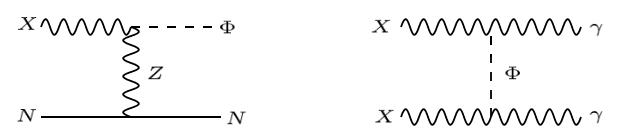
Figure 12: Left: Inelastic DM scattering off the nuclei $N$ for direct search of DM; right: DM annihilating to photon final states via $\Phi$ mediation for indirect search of DM.

As we have already demonstrated, the dimensionful $\Phi-B-X$ vertex ($\alpha(\tilde{\alpha})$) is constrained by relic density of DM to be $\alpha(\tilde{\alpha})\lesssim 10^{-12}~{}\text{GeV}^{-1}$ for $T_{\text{RH}}\gtrsim 10^{3}$ GeV. Therefore, assuming $c\sim{\cal O}(1)$ , one can conclude that freeze-in of the VDM requires the NP scale $\Lambda\mbox{\raisebox{-2.58334pt}{~{}$\stackrel{{\scriptstyle>}}{{\sim}}$~{}}}10^{12}$ GeV at least or higher for larger reheat temperature. If the effective operators (50) where $n$-loop generated, then we would roughly conclude that $\Lambda\mbox{\raisebox{-2.58334pt}{~{}$\stackrel{{\scriptstyle>}}{{\sim}}$~{}}}10^{12-2n}\;\text{GeV}$. Hereafter we assume that the Lagrangian (50) is indeed tree-level generated. Therefore, the phenomenology of the model is severely constrained. First of all, note that there is no $XX-SM$ vertex, therefore no elastic scattering of the DM against nuclei is possible. So, this model easily avoids stringent constraints from non-observation of DM scattering at direct search experiments. DM can only scatter off nuclei inelastically with $\Phi$ in the final state as shown in left panel of Fig. 12. Since $m_{\Phi}>m_{X}$, hence such an inelastic scattering is forbidden even if the mass difference $\delta m=m_{\Phi}-m_{X}\gtrsim\mathcal{O}(100)~{}\rm MeV$ TuckerSmith:2001hy . On the other hand, due to the presence of $\Phi-X-\gamma$ vertex, the DM pair annihilation may give rise to monochromatic X-ray line (right panel of Fig. 12) but such photon flux will be hugely suppressed by $1/\Lambda^{2}$ and can not account for the, say, galactic-center gamma ray excess as observed. Hence this model in its freeze-in realization of DM can not be probed from either direct nor indirect DM search experiments.

  

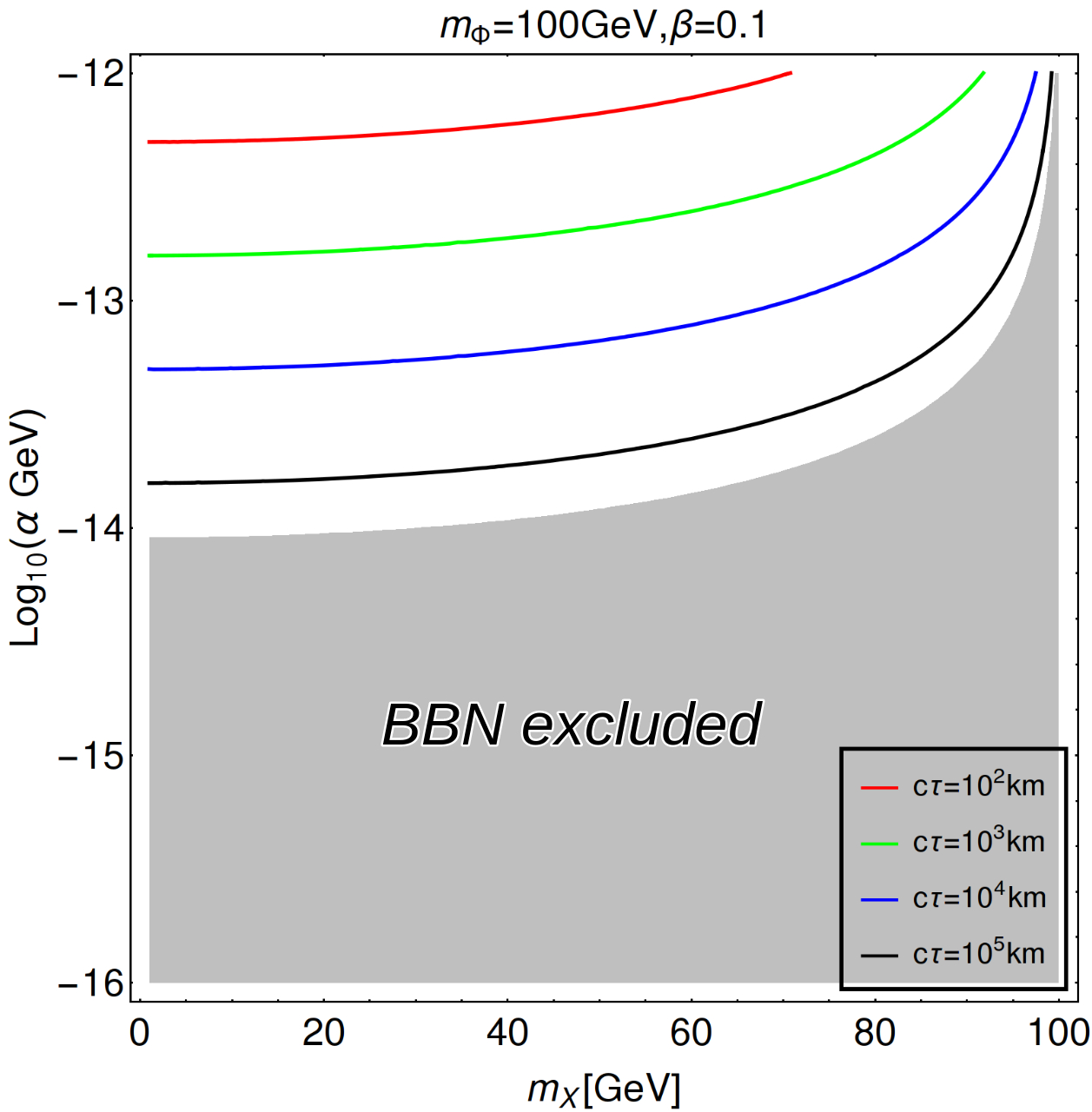
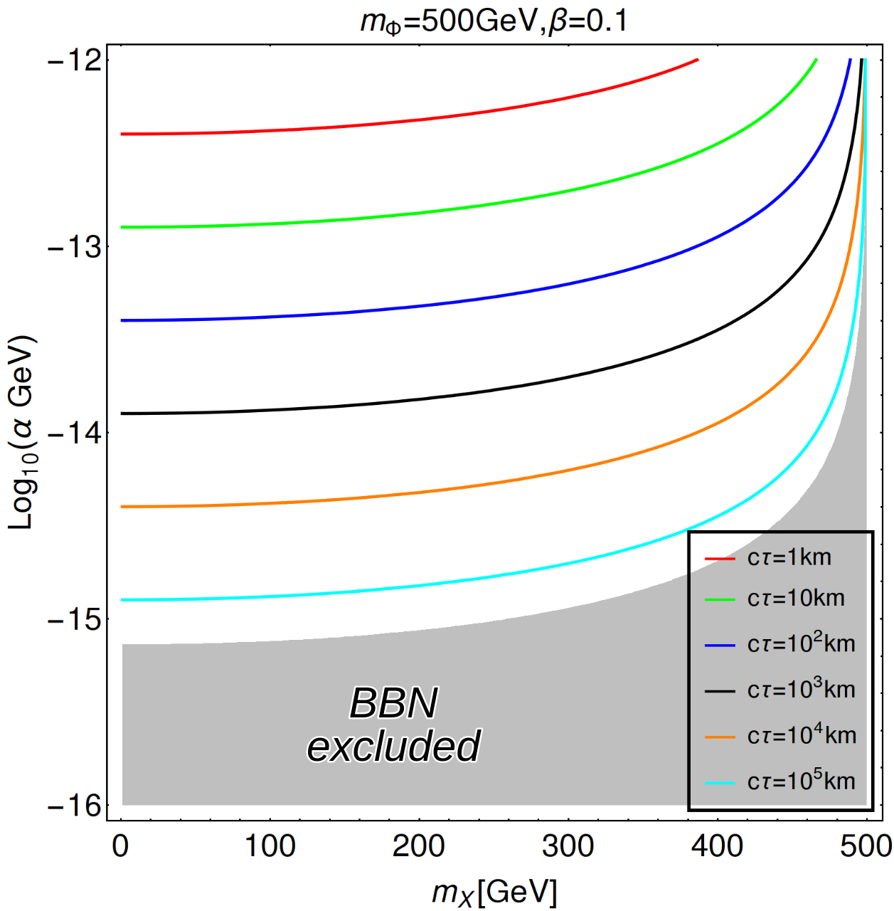
Figure 13: The contours show different decay lengths of $\Phi$ for particular choices of the parameters that can produce right relic abundance for the DM. On left panel, we choose $m_{\Phi}=100$ GeV, while on the right panel we show the case for $m_{\Phi}=500$ GeV. The shaded region at the bottom is excluded by BBN constraint $\tau_{\Phi}\mbox{\raisebox{-2.58334pt}{~{}$\stackrel{{\scriptstyle<}}{{\sim}}$~{}}}\tau_{\text{BBN}}\sim 1~{}\sec$.

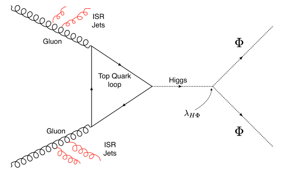
Figure 14: $\not{E}_{T}+\text{jets}$ signature that the model can produce at the collider.

However, since the portal coupling $\lambda_{H\Phi}$ is unconstrained by existing observations and as argued before this coupling can be as large as $\lambda_{H\phi}\sim\mathcal{O}(1)$, hence the non-standard scalar $\Phi$ can be produced at the collider via Higgs mediation (see Fig. 14). Once these $\phi$’s get produced at colliders they will eventually decay via Fig. 2 to DM and SM final states like $Z,\gamma$. This is the same channel that also gives rise to DM production via freeze-in. For particular choice of the effective coupling $\alpha$ that gives rise to right relic abundance, the $\Phi$ remain stable over the detector length. This is shown in Fig. 13, where we see that for $\alpha=10^{-14}-10^{-13}\;\text{GeV}^{-1}$ the average decay length of $\Phi$ is $L_{\Phi}=c\tau_{\Phi}\gtrsim 100~{}\rm km$, where $c=3\times 10^{8}~{}\text{ m/sec}$. In such a case the $\Phi$’s basically escapes LHC detector and gives rise to missing energy $(\not{E}_{T})$, which can be constructed out of the recoil of an initial state radiation (ISR) of a gluon, $\gamma$, $W^{\pm},Z,H$ as

$$\not{E}_{T}=-\sqrt{\left(\sum_{\ell,j}p_{x}\right)^{2}+\left(\sum_{\ell,j}p_{y}\right)^{2}},$$ (84)

where the sum runs over all visible objects that include leptons and jets, and unclustered components. Therefore, the model can finally produce monojet  plus missing energy signal that has extensively been searched at the LHC Chala:2015ama ; Aaboud:2016uro ; Aaboud:2016tnv as a vanilla DM signal particularly for Higgs portal DM models. However, usually, when one produces DM that is connected with the SM via a Higgs portal, then the coupling is tightly constrained from direct search. Therefore, such signals are pretty small and submerged into huge SM background. In our case, as mentioned, the coupling ($\lambda_{H\phi}$) can be large and can produce a significant number of such mono-X signal events, that may be of interest for next run of LHC.

It is worth noting that decays of $\Phi$ have to be completed before the onset of Big Bang Nucleosynthesis (BBN) Kolb:1990vq ; PhysRevD.98.030001 , so that it does not alter the standard BBN picture. Therefore here we will require that $\tau_{\Phi}\mbox{\raisebox{-2.58334pt}{~{}$\stackrel{{\scriptstyle<}}{{\sim}}$~{}}}\tau_{\text{BBN}}\sim 1~{}\sec$ which, for fixed $m_{\Phi}$ and $m_{X}<m_{\Phi}$ puts a lower bound on $\alpha$. This has been illustrated in Fig. 14 where we show, for $m_{\Phi}=100\;\text{GeV}$ and $500\;\text{GeV}$, regions allowed by the BBN constraint ($c\tau=10^{5}$ km). Concluding one can see that usually $\alpha\mbox{\raisebox{-2.58334pt}{~{}$\stackrel{{\scriptstyle>}}{{\sim}}$~{}}}10^{-15}\;\text{GeV}$ is allowed, while the region $m_{X}\sim m_{\Phi}$ is forbidden for any value of $\alpha$.

6 Summary and Conclusions

A vector boson DM weakly coupled to the visible SM sector via dimension-5 operator has been presented and the parameter space allowed by observed relic DM density has been found. The advantage of the model is the absence of tree-level elastic DM scattering against nuclei and a double suppression of present time DM annihilation in, for instance, dwarf galaxies. Therefore this scenario easily and naturally satisfies existing experimental constraints. The model contains a dark sector composed, in a unitary gauge, of a massive vector $X_{\mu}$, and a real scalar $\Phi$. $X_{\mu}$ is a gauge boson of spontaneously broken extra $U(1)_{X}$ gauge symmetry. The vector $X_{\mu}$ and the scalar $\Phi$ are odd under a $Z_{2}$ symmetry introduced to stabilize the DM candidate, $X_{\mu}$. $\Phi$ is assumed to be heavier than $X_{\mu}$. The SM sector is extended by an extra heavy neutral Higgs boson that decouples when its mass goes to infinity, as we assume here. The lowest dimensional operator responsible for DM-SM interaction are $1/\Lambda\;X^{\mu\nu}B_{\mu\nu}\Phi$ and $1/\Lambda\;\tilde{X}^{\mu\nu}B_{\mu\nu}\Phi$. It has been shown that the model can be formulated in a Stueckelberg-like fashion as a limit of the SM extended by the $U(1)_{X}$ gauge symmetry together with a complex scalar charged under the $U(1)_{X}$ (needed to spontaneously break the symmetry) and a real scalar $\Phi$.

We have investigated a possibility of DM production via a freeze-in mechanism through decays of $\Phi$ and annihilations including $\Phi$. It turned out to be convenient to consider two distinct regimes of the reheat temperature. The first one is when the reheat temperature is significantly higher than masses involved in the production process. This situation mimics the case of UV freeze-in, when the production happens mostly before EWSB and all processes after EWSB are insignificant. However the situation alters, when reheat temperature (which can be thought of a free parameter, being very loosely constrained by BBN) drops to lower values close to the mass scale ($m$) typical for the dark sector. It has been shown that UV freeze-in, although advertised to describe the case of freeze-in production of DM in EFT formalism, is not fully correct, massive contributions start playing an important role and effects of IR freeze-in i.e. DM yield building even up to lower temperature ($T\sim m$) starts showing up.

In order to predict properly the observed DM abundance, the scale of the dimension-5 operators must be large $\Lambda\sim 10^{12}-10^{16}\;\text{GeV}$ depending on the DM mass $m_{X}$, the reheat temperature $T_{\text{RH}}$ and an underlying mechanism for the generation of the relevant effective operators. The huge size of $\Lambda$ implies that at the lowest level of perturbative expansion neither elastic scattering off nuclei is allowed nor present time annihilations of DM in e.g. centers of galaxies are possible. However, it turns out that LHC collider signals mediated by Higgs boson exchange are possible, $gg\to H^{*}\to\Phi\Phi$. Since the scale of $\Lambda$ required by the DM abundance is large $\Lambda\sim 10^{12}-10^{16}\;\text{GeV}$ the heavier scalar $\Phi$ is effectively stable at the detector length scale and hence can produce mono-jet, photon, $Z,W^{\pm}$ or $H$ events accompanied by missing energy drifted away by pairs of $\Phi$ bosons.The signal cross-section could be quite substantial as the portal coupling between $\Phi$ and the SM remains unconstrained.

Finally, we must mention that a freeze-out possibility of the same model can also be thought of. In that case, the phenomenological signatures will become richer. In contrast to the case considered here the freeze-out scenario implies constraints that are more difficult to satisfy Fortuna:2020wwx .

Acknowledgement
SB would like to acknowledge DST-SERB grant CRG/2019/004078 and WHEPP meeting at IIT Guwahati, where the work was initiated. BB and SB would like to thank Sunando Patra for helping out with numerical computations. The work of B.G. is supported in part by the National Science Centre (Poland) as a research project, decision no 2017/25/B/ST2/00191.

Appendix A The parameters of the scalar potential

Here we collect useful relations between potential parameters.

$$\begin{split}m_{1}^{2}&=\sec(2\alpha)\left(2\lambda_{H}v_{h}^{2}\cos^{2}\alpha-2\lambda_{S}v_{S}^{2}\sin^{2}\alpha\right),\\ m_{2}^{2}&=\sec(2\alpha)\left(2\lambda_{S}v_{S}^{2}\cos^{2}\alpha-2\lambda_{H}v_{h}^{2}\sin^{2}\alpha\right),\\ m_{\Phi}^{2}&=2\mu_{\Phi}^{2}+\lambda_{H\Phi}v_{h}^{2}+\lambda_{S\Phi}v_{S}^{2}.\end{split}$$ (85)

The couplings, likewise, can be expressed in terms of the physical masses and mixing:

$$\begin{split}\lambda_{H}=\frac{m_{1}^{2}\cos^{2}\alpha+m_{2}^{2}\sin^{2}\alpha}{2v_{h}^{2}},~{}\lambda_{S}=\frac{m_{1}^{2}\sin^{2}\alpha+m_{2}^{2}\cos^{2}\alpha}{2v_{S}^{2}},\\ \lambda_{SH}=\frac{\sin\alpha\cos\alpha\left(m_{1}^{2}-m_{2}^{2}\right)}{v_{h}v_{S}},~{}\lambda_{S\Phi}=\frac{-2\mu_{\Phi}^{2}+m_{3}^{2}-\lambda_{H\Phi}v_{h}^{2}}{v_{S}^{2}},\\ \end{split}$$ (86)

with,

$$\sin\left(2\alpha\right)=\left(\frac{2v_{h}v_{S}}{m_{1}^{2}-m_{2}^{2}}\right)\lambda_{SH}.$$ (87)

Now, from Eq. (85) we see:

$$m_{1}^{2}+m_{2}^{2}=2\left(\lambda_{H}v_{h}^{2}+\lambda_{S}v_{S}^{2}\right).$$ (88)

From (28-88) we find a useful expression for $m_{2}$:

$$m_{2}^{2}=v_{h}^{2}\frac{2(\lambda_{H}-\lambda_{SM})(4\lambda_{H}\lambda_{S}-\lambda_{SH}^{2})}{4\lambda_{S}(\lambda_{H}-\lambda_{SM})-\lambda_{SH}^{2}}$$ (89)

Appendix B Relevant vertices

Adopting the Lagrangian of the model in Eq. (2.5), one finds relevant vertices and propagators collected in the table 3. Here the notation have usual meaning, for example, $g_{1,2}$ are the gauge couplings corresponding to $U(1)_{Y}$ and $SU(2)_{L}$ gauge groups, respectively. $c_{v}$ and $c_{a}$ are defined as: $c_{v}^{f}=T_{3L}-2\sin^{2}\theta_{w}Q_{f}$ and $c_{a}^{f}=T_{3L}$, where $T_{3L}$ is the $SU(2)_{L}$ isospin quantum number and $Q_{f}$ is the charge of the SM fermion $f$ concerned.

Vertex	Vertex factors
	$i\tilde{\alpha}\varepsilon_{\mu\nu\rho\sigma}p_{1}^{\rho}p_{2}^{\sigma}+i\alpha\left(\eta_{\mu\nu}p_{1}.p_{2}-p_{1_{\nu}}p_{2_{\mu}}\right)$
	$-\frac{ig_{1}}{2}\left(p_{2}-p_{4}\right)_{\mu}$
	$-ie\left[\left(k_{1}-k_{2}\right)_{a}g_{bc}+\left(k_{2}-k_{3}\right)_{b}g_{ac}+\left(k_{1}-k_{3}\right)_{c}g_{ab}\right]$
	$-ig_{2}c_{w}\left[\left(k_{1}-k_{2}\right)_{a}g_{bc}+\left(k_{2}-k_{3}\right)_{b}g_{ac}+\left(k_{1}-k_{3}\right)_{c}g_{ab}\right]$
$f\overline{f}B_{\mu}$	$\frac{ig_{1}}{2}\gamma^{\mu}\frac{1}{2}\begin{cases}\left(Y_{L}^{\ell}+Y_{R}^{\ell}\right)-\gamma_{5}\left(Y_{L}^{\ell}-Y_{R}^{\ell}\right)&\\ \left(Y_{L}^{Q}+Y_{R}^{Q}\right)-\gamma_{5}\left(Y_{L}^{Q}-Y_{R}^{Q}\right)&\end{cases}$
$h\Phi\Phi$	$2i\lambda_{H\Phi}v_{h}$
$hZZ$	$\frac{iv_{h}}{4}\left(g_{1}^{2}+g_{2}^{2}\right)$
$f\overline{f}Z_{\mu}$	$-i\frac{g_{2}}{c_{w}}\gamma_{\mu}\frac{1}{2}\begin{cases}\left(c_{v}^{\ell}-c_{a}^{\ell}\gamma_{5}\right)&\\ \left(c_{v}^{Q}-c_{a}^{Q}\gamma_{5}\right)&\end{cases}$
$f\overline{f}\gamma$	$-ieQ_{f}\gamma_{\mu}$
Propagator	$R_{\xi}$ gauge Feynman rules
	$\frac{i}{k^{2}-m_{Z}^{2}}\Biggl{[}-g_{\mu\nu}+\left(1-\xi\right)\frac{k_{\mu}k_{\nu}}{k^{2}-\xi m_{Z}^{2}}\Biggr{]}$
	$\frac{i}{k^{2}}\Biggl{[}-g_{\mu\nu}+\left(1-\xi\right)\frac{k_{\mu}k_{\nu}}{k^{2}}\Biggr{]}$

Table 3: Relevant DM-SM interaction vertices and vertex factors along with SM propagators. All momenta are assumed flowing towards the vertices. Here $\ell$ stands for SM leptons and $Q$ stands for the SM quark generations. $Y_{L,R}^{\ell(Q)}$ is the hypercharge for left and right-chiral leptons (quarks): $Y_{L}^{\nu}=-1,Y_{L}^{e}=-1,Y_{R}^{e}=-2;Y_{L}^{Q}=1/3,Y_{R}^{u}=4/3,Y_{R}^{d}=-2/3$.

Appendix C Reaction densities

For a $2\to 2$ annihilation channel the reaction density is defined as:

$$\begin{split}\gamma\left(a,b\to 1,2\right)&=\int\prod_{i=1}^{4}d\Pi_{i}\left(2\pi\right)^{4}\delta^{(4)}\biggl{(}p_{a}+p_{b}-p_{1}-p_{2}\biggr{)}f_{a}^{eq}f_{b}^{eq}\left|\mathcal{M}_{a,b\to 1,2}\right|^{2}\\ &=\frac{T}{32\pi^{4}}g_{a}g_{b}\int_{s_{min}}^{\infty}ds~{}\frac{\biggl{[}\bigl{(}s-m_{a}^{2}-m_{b}^{2}\bigr{)}^{2}-4m_{a}^{2}m_{b}^{2}\biggr{]}}{\sqrt{s}}\sigma\left(s\right)_{a,b\to 1,2}K_{1}\left(\frac{\sqrt{s}}{T}\right),\end{split}$$ (90)

where $a,b(1,2)$ are the incoming (outgoing) states and $g_{a,b}$ are corresponding degrees of freedom. Here $f_{i}^{eq}\approx\exp^{-E_{i}/T}$ is the Maxwell-Boltzmann distribution. The Lorentz invarint 2-body phase space is denoted by: $d\Pi_{i}=\frac{d^{3}p_{i}}{\left(2\pi\right)^{3}2E_{i}}$. The amplitude squared (summed over final and averaged over initial states) is denoted by $\left|\mathcal{M}_{a,b\to 1,2}\right|^{2}$ for a particular $2\to 2$ scattering process. The lower limit of the integration over $s$ is $s_{min}=\text{max}\biggl{[}\left(m_{a}+m_{b}\right)^{2},\left(m_{1}+m_{2}\right)^{2}\biggr{]}$.

For a $1\to 2$ decay process the reaction density is given by:

$$\begin{split}\gamma\left(a\to 1,2\right)&=\int\sum_{i=1}^{3}d\Pi_{i}\left(2\pi\right)^{4}\delta^{(4)}\biggl{(}p_{a}-p_{1}-p_{2}\biggr{)}f_{a}^{eq}\left|\mathcal{M}_{a\to 1,2}\right|^{2}\\ &=\frac{g_{a}}{2\pi^{2}}m_{a}^{2}\Gamma_{a\to 1,2}TK_{1}\left(\frac{m_{a}}{T}\right).\end{split}$$ (91)

Appendix D Expressions for squared amplitudes before EWSB

D.1 t-channel annihilation before EWSB

The spin averaged amplitude squared for $f\Phi\to fX$ process is given by:

$$\begin{split}\left|\overline{\mathcal{M}}\right|^{2}_{f\Phi\to fX}&=\frac{g_{1}^{2}N_{c}}{128s\left(s-m_{X}^{2}\right)\left(s-m_{\Phi}^{2}\right)\big{(}\cos\theta-1\big{)}}\left(\left[Y_{L}^{f}+Y_{R}^{f}\right]^{2}+\left[Y_{L}^{f}-Y_{R}^{f}\right]^{2}\right)\\ &\Biggl{[}\alpha^{2}\Bigl{(}1+\beta^{2}\Bigr{)}\Bigg{\{}4\cos\theta\left(s-m_{X}^{2}\right)\left(m_{\Phi}^{2}-s\right)\left[3s^{2}+s\left(m_{\Phi}^{2}-5m_{X}^{2}\right)+m_{X}^{2}m_{\Phi}^{2}\right]\\ &+\cos 2\theta\left(s-m_{X}^{2}\right)^{2}\left(s-m_{\Phi}^{2}\right)^{2}+s\Bigl{(}2m_{X}^{2}m_{\Phi}^{4}-22m_{X}^{4}m_{\Phi}^{2}\Bigr{)}\\ &+s^{2}\Bigl{(}27m_{X}^{4}-4m_{X}^{2}m_{\Phi}^{2}+3m_{\Phi}^{4}\Bigr{)}+s^{3}\Bigl{(}10m_{\Phi}^{2}-14m_{X}^{2}\Bigr{)}-5s^{4}\Bigg{\}}\\ &+\alpha^{2}\Bigl{(}1-\beta^{2}\Bigr{)}\Bigg{\{}16m_{X}^{2}s\sin^{2}\left(\frac{\theta}{2}\right)\left(m_{X}^{2}-s\right)\left(m_{\Phi}^{2}-s\right)\Bigg{\}}\Biggr{]},\end{split}$$ (92)

where $N_{c}=1(3)$ for the SM leptons (quarks). Also note that all the SM fermions are massless. In the limit $m_{\Phi}=m_{X}=0$ this reduces to a relatively simplified form:

$$\left|\overline{\mathcal{M}}\right|^{2}_{f,\Phi\to f,X}=g_{1}^{2}N_{c}s\alpha^{2}\left(1+\beta^{2}\right)\left(\left[Y_{L}^{f}+Y_{R}^{f}\right]^{2}+\left[Y_{L}^{f}-Y_{R}^{f}\right]^{2}\right)\left(\frac{5+12\cos\theta-\cos 2\theta}{128(1-\cos\theta)}\right).$$ (93)

Corresponding annihilation cross-section is given by:

$$\begin{split}&\sigma\left(s\right)_{f\Phi\to fX}\simeq\frac{6g_{1}^{2}N_{c}}{25}\alpha^{2}\left(1+\beta^{2}\right)\left(\left[Y_{L}^{f}+Y_{R}^{f}\right]^{2}+\left[Y_{L}^{f}-Y_{R}^{f}\right]^{2}\right).\end{split}$$ (94)

D.2 s-channel annihilation before EWSB

The spin averaged amplitude squared for $ff\to X\Phi$ process is given by:

$$\begin{split}\left|\overline{\mathcal{M}}\right|^{2}_{f,f\to\Phi,X}&=\frac{g_{1}^{2}N_{c}}{256s^{3}}\left(\left[Y_{L}^{f}+Y_{R}^{f}\right]^{2}+\left[Y_{L}^{f}-Y_{R}^{f}\right]^{2}\right)\\ &\Biggl{[}\alpha^{2}\Bigl{(}1+\beta^{2}\Bigr{)}\Bigg{\{}3m_{X}^{4}m_{\Phi}^{4}-2m_{X}^{4}m_{\Phi}^{2}s+3m_{X}^{4}s^{2}+2m_{X}^{2}m_{\Phi}^{4}s\\ &-4m_{\Phi}^{2}\cos\theta\left(m_{X}^{2}-s\right)\left(m_{X}^{2}+s\right)\left(m_{\Phi}^{2}-s\right)+\cos 2\theta\left(s-m_{X}^{2}\right)^{2}\left(s-m_{\Phi}^{2}\right)^{2}\\ &+2m_{X}^{2}s^{3}+3m_{\Phi}^{4}s^{2}-6m_{\Phi}^{2}s^{3}+3s^{4}\Bigg{\}}+8\alpha^{2}\Bigl{(}1-\beta^{2}\Bigr{)}m_{X}^{2}s^{3}\Biggr{]},\end{split}$$ (95)

with $N_{c}=1(3)$ for SM leptons (quarks). In the limit $m_{X}=m_{\Phi}=0$ this reduces to:

$$\left|\overline{\mathcal{M}}\right|^{2}_{ff\to\Phi,X}=\frac{g_{1}^{2}N_{c}}{64}s\alpha^{2}\left(1+\beta^{2}\right)(\cos 2\theta+3)\left(\left[Y_{L}^{f}+Y_{R}^{f}\right]^{2}+\left[Y_{L}^{f}-Y_{R}^{f}\right]^{2}\right),$$ (96)

Corresponding annihilation cross-section is given by:

$$\begin{split}&\sigma\left(s\right)_{ff\to\Phi X}\simeq\frac{g_{1}^{2}N_{c}}{1000}\alpha^{2}\left(1+\beta^{2}\right)\left(\left[Y_{L}^{f}+Y_{R}^{f}\right]^{2}+\left[Y_{L}^{f}-Y_{R}^{f}\right]^{2}\right).\end{split}$$ (97)

D.3 Decay of $\Phi$

D.3.1 Before EWSB

The amplitude squared for the $\Phi\to X,B$ decay is given by:

$$\left|\mathcal{M}\right|_{\text{D}}^{2}=\frac{m_{\Phi}^{4}}{2}\alpha^{2}\left(1+\beta^{2}\right)\left(1-r^{2}\right)^{2}.$$ (98)

The resulting decay width can be written as:

$$\Gamma_{\Phi\to X,B}=\frac{m_{\Phi}^{3}}{32\pi}\alpha^{2}\left(1+\beta^{2}\right)\left(1-r^{2}\right)^{3},$$ (99)

D.3.2 After EWSB

After EWSB $\Phi$ decays to photon and $Z$ final states resulting:

$$\Gamma_{\text{total}}=\Gamma_{\Phi\to X,Z}+\Gamma_{\Phi\to X,\gamma}.$$ (100)

The squared amplitude for decay to photon and massive $Z$-boson final state takes the form:

$$\begin{split}\left|\mathcal{M}\right|^{2}_{\text{total}}&=\underbrace{\frac{m_{\Phi}^{4}}{2}\alpha^{2}\left(1+\beta^{2}\right)\left(1-r^{2}\right)^{2}c_{w}^{2}}_{\text{due to photon}}\\ &+\underbrace{\frac{1}{2}\alpha^{2}s_{w}^{2}\Bigl{[}m_{\Phi}^{4}\left(1+\beta^{2}\right)\left(1-r^{2}-y^{2}\right)^{2}-4\beta^{2}m_{X}^{2}m_{Z}^{2}+2m_{X}^{2}m_{Z}^{2}\Bigr{]}}_{\text{due to massive $Z$-boson}}\end{split}$$ (101)

Thus, the total decay width after EWSB can be expressed as:

$$\begin{split}\Gamma_{\text{total}}&=\frac{\alpha^{2}m_{\Phi}^{3}\left(1+\beta^{2}\right)}{32\pi}\biggl{[}c_{w}^{2}\left(1-r^{2}\right)^{3}+s_{w}^{2}\left(r^{4}-2r^{2}+\left(y^{2}-1\right)^{2}\right)\\ &\sqrt{1-\left(r-y\right)^{2}}\sqrt{1-\left(r+y\right)^{2}}\biggr{]},\end{split}$$ (102)

where $0<r=m_{X}/m_{\Phi}\leq 1$ and $0<y=m_{Z}/m_{\Phi}\leq 1$.

References

- (1) F. Zwicky, Die Rotverschiebung von extragalaktischen Nebeln, Helv. Phys. Acta 6 (1933) 110–127. [Gen. Rel. Grav.41,207(2009)].
- (2) F. Zwicky, On the Masses of Nebulae and of Clusters of Nebulae, Astrophys. J. 86 (1937) 217–246.
- (3) V. C. Rubin and W. K. Ford, Jr., Rotation of the Andromeda Nebula from a Spectroscopic Survey of Emission Regions, Astrophys. J. 159 (1970) 379–403.
- (4) D. Clowe, M. Bradac, A. H. Gonzalez, M. Markevitch, S. W. Randall, C. Jones, and D. Zaritsky, A direct empirical proof of the existence of dark matter, Astrophys. J. Lett. 648 (2006) L109–L113, [astro-ph/0608407].
- (5) R. Massey, T. Kitching, and J. Richard, The dark matter of gravitational lensing, Rept. Prog. Phys. 73 (2010) 086901, [arXiv:1001.1739].
- (6) W. Hu and S. Dodelson, Cosmic microwave background anisotropies, Ann. Rev. Astron. Astrophys. 40 (2002) 171–216, [astro-ph/0110414].
- (7) G. Bertone, D. Hooper, and J. Silk, Particle dark matter: Evidence, candidates and constraints, Phys. Rept. 405 (2005) 279–390, [hep-ph/0404175].
- (8) J. L. Feng, Dark Matter Candidates from Particle Physics and Methods of Detection, Ann. Rev. Astron. Astrophys. 48 (2010) 495–545, [arXiv:1003.0904].
- (9) WMAP Collaboration, D. N. Spergel et al., Wilkinson Microwave Anisotropy Probe (WMAP) three year results: implications for cosmology, Astrophys. J. Suppl. 170 (2007) 377, [astro-ph/0603449].
- (10) N. Jarosik et al., Seven-Year Wilkinson Microwave Anisotropy Probe (WMAP) Observations: Sky Maps, Systematic Errors, and Basic Results, Astrophys. J. Suppl. 192 (2011) 14, [arXiv:1001.4744].
- (11) WMAP Collaboration, G. Hinshaw et al., Nine-Year Wilkinson Microwave Anisotropy Probe (WMAP) Observations: Cosmological Parameter Results, Astrophys. J. Suppl. 208 (2013) 19, [arXiv:1212.5226].
- (12) Planck Collaboration, P. A. R. Ade et al., Planck 2013 results. XVI. Cosmological parameters, Astron. Astrophys. 571 (2014) A16, [arXiv:1303.5076].
- (13) Planck Collaboration, N. Aghanim et al., Planck 2018 results. VI. Cosmological parameters, arXiv:1807.06209.
- (14) E. W. Kolb and M. S. Turner, The Early Universe, Front. Phys. 69 (1990) 1–547.
- (15) G. Jungman, M. Kamionkowski, and K. Griest, Supersymmetric dark matter, Phys. Rept. 267 (1996) 195–373, [hep-ph/9506380].
- (16) H. Baer, K.-Y. Choi, J. E. Kim, and L. Roszkowski, Dark matter production in the early Universe: beyond the thermal WIMP paradigm, Phys. Rept. 555 (2015) 1–60, [arXiv:1407.0017].
- (17) G. Arcadi, M. Dutra, P. Ghosh, M. Lindner, Y. Mambrini, M. Pierre, S. Profumo, and F. S. Queiroz, The waning of the WIMP? A review of models, searches, and constraints, Eur. Phys. J. C 78 (2018), no. 3 203, [arXiv:1703.07364].
- (18) L. J. Hall, K. Jedamzik, J. March-Russell, and S. M. West, Freeze-In Production of FIMP Dark Matter, JHEP 03 (2010) 080, [arXiv:0911.1120].
- (19) Y. Farzan and A. R. Akbarieh, VDM: A model for Vector Dark Matter, JCAP 1210 (2012) 026, [arXiv:1207.4272].
- (20) S. Baek, P. Ko, W.-I. Park, and E. Senaha, Higgs Portal Vector Dark Matter : Revisited, JHEP 05 (2013) 036, [arXiv:1212.2131].
- (21) L. Bian, R. Ding, and B. Zhu, Two Component Higgs-Portal Dark Matter, Phys. Lett. B728 (2014) 105–113, [arXiv:1308.3851].
- (22) S. Y. Choi, C. Englert, and P. M. Zerwas, Multiple Higgs-Portal and Gauge-Kinetic Mixings, Eur. Phys. J. C73 (2013) 2643, [arXiv:1308.5784].
- (23) S. Baek, P. Ko, and W.-I. Park, Hidden sector monopole, vector dark matter and dark radiation with Higgs portal, JCAP 1410 (2014), no. 10 067, [arXiv:1311.1035].
- (24) S. Baek, H. Okada, and T. Toma, Two loop neutrino model and dark matter particles with global B-L symmetry, JCAP 1406 (2014) 027, [arXiv:1312.3761].
- (25) P. Ko, W.-I. Park, and Y. Tang, Higgs portal vector dark matter for scale -ray excess from galactic center, JCAP 1409 (2014) 013, [arXiv:1404.5257].
- (26) S. Baek, P. Ko, and W.-I. Park, The 3.5 keV X-ray line signature from annihilating and decaying dark matter in Weinberg model, arXiv:1405.3730.
- (27) P. Ko and Y. Tang, Galactic center -ray excess in hidden sector DM models with dark gauge symmetries: local symmetry as an example, JCAP 1501 (2015) 023, [arXiv:1407.5492].
- (28) M. Duch, B. Grzadkowski, and M. McGarrie, A stable Higgs portal with vector dark matter, JHEP 09 (2015) 162, [arXiv:1506.08805].
- (29) A. Beniwal, F. Rajec, C. Savage, P. Scott, C. Weniger, M. White, and A. G. Williams, Combined analysis of effective Higgs portal dark matter models, Phys. Rev. D93 (2016), no. 11 115016, [arXiv:1512.06458].
- (30) T. Kamon, P. Ko, and J. Li, Characterizing Higgs portal dark matter models at the ILC, Eur. Phys. J. C77 (2017), no. 9 652, [arXiv:1705.02149].
- (31) M. Duch and B. Grzadkowski, Resonance enhancement of dark matter interactions: the case for early kinetic decoupling and velocity dependent resonance width, JHEP 09 (2017) 159, [arXiv:1705.10777].
- (32) G. Arcadi, P. Ghosh, Y. Mambrini, M. Pierre, and F. S. Queiroz, portal to Chern-Simons Dark Matter, JCAP 1711 (2017), no. 11 020, [arXiv:1706.04198].
- (33) S. Baek and C. Yu, Dark matter for anomaly in a gauged model, JHEP 11 (2018) 054, [arXiv:1806.05967].
- (34) S. Yaser Ayazi and A. Mohamadnejad, Conformal vector dark matter and strongly first-order electroweak phase transition, JHEP 03 (2019) 181, [arXiv:1901.04168].
- (35) M. Duch, B. Grzadkowski, and D. Huang, Strongly self-interacting vector dark matter via freeze-in, JHEP 01 (2018) 020, [arXiv:1710.00320].
- (36) G. Choi, T. T. Yanagida, and N. Yokozaki, Feebly Interacting Gauge Boson Warm Dark Matter and XENON1T Anomaly, arXiv:2007.04278.
- (37) G. Choi, T. T. Yanagida, and N. Yokozaki, Dark Photon Dark Matter in the minimal Model, arXiv:2008.12180.
- (38) J. L. Diaz-Cruz and E. Ma, Neutral gauge extension of the standard model and a vector-boson dark-matter candidate, Physics Letters B 695 (2011), no. 1 264 – 267.
- (39) J. Diaz-Cruz and E. Ma, Neutral SU(2) Gauge Extension of the Standard Model and a Vector-Boson Dark-Matter Candidate, Phys. Lett. B 695 (2011) 264–267, [arXiv:1007.2631].
- (40) S. Bhattacharya, J. L. Diaz-Cruz, E. Ma, and D. Wegman, Dark Vector-Gauge-Boson Model, Phys. Rev. D85 (2012) 055008, [arXiv:1107.2093].
- (41) Y. Farzan and A. R. Akbarieh, Natural explanation for 130 GeV photon line within vector boson dark matter model, Phys. Lett. B 724 (2013) 84–87, [arXiv:1211.4685].
- (42) B. Barman, S. Bhattacharya, S. K. Patra, and J. Chakrabortty, Non-Abelian Vector Boson Dark Matter, its Unified Route and signatures at the LHC, JCAP 1712 (2017), no. 12 021, [arXiv:1704.04945].
- (43) S. Fraser, E. Ma, and M. Zakeri, model of vector dark matter with a leptonic connection, Int. J. Mod. Phys. A30 (2015), no. 03 1550018, [arXiv:1409.1162].
- (44) B. Barman, S. Bhattacharya, and M. Zakeri, Multipartite Dark Matter in extension of Standard Model and signatures at the LHC, JCAP 1809 (2018), no. 09 023, [arXiv:1806.01129].
- (45) B. Barman, S. Bhattacharya, and M. Zakeri, Non-Abelian Vector Boson as FIMP Dark Matter, JCAP 2002 (2020), no. 02 029, [arXiv:1905.07236].
- (46) T. Abe, M. Fujiwara, J. Hisano, and K. Matsushita, A model of electroweakly interacting non-abelian vector dark matter, JHEP 07 (2020) 136, [arXiv:2004.00884].
- (47) S. Profumo, An Introduction to Particle Dark Matter. World Scientific, 2017.
- (48) L. Roszkowski, E. M. Sessolo, and S. Trojanowski, WIMP dark matter candidates and searches—current status and future prospects, Rept. Prog. Phys. 81 (2018), no. 6 066201, [arXiv:1707.06277].
- (49) X. Chu, T. Hambye, and M. H. G. Tytgat, The Four Basic Ways of Creating Dark Matter Through a Portal, JCAP 1205 (2012) 034, [arXiv:1112.0493].
- (50) F. Elahi, C. Kolda, and J. Unwin, UltraViolet Freeze-in, JHEP 03 (2015) 048, [arXiv:1410.6157].
- (51) R. T. Co, F. D’Eramo, L. J. Hall, and D. Pappadopulo, Freeze-In Dark Matter with Displaced Signatures at Colliders, JCAP 1512 (2015), no. 12 024, [arXiv:1506.07532].
- (52) N. Bernal, M. Heikinheimo, T. Tenkanen, K. Tuominen, and V. Vaskonen, The Dawn of FIMP Dark Matter: A Review of Models and Constraints, Int. J. Mod. Phys. A32 (2017), no. 27 1730023, [arXiv:1706.07442].
- (53) S. Heeba, F. Kahlhoefer, and P. Stöcker, Freeze-in production of decaying dark matter in five steps, JCAP 1811 (2018), no. 11 048, [arXiv:1809.04849].
- (54) S. Peyman Zakeri, S. Mohammad Moosavi Nejad, M. Zakeri, and S. Yaser Ayazi, A Minimal Model For Two-Component FIMP Dark Matter: A Basic Search, Chin. Phys. C42 (2018), no. 7 073101, [arXiv:1801.09115].
- (55) M. Becker, Dark Matter from Freeze-In via the Neutrino Portal, Eur. Phys. J. C79 (2019), no. 7 611, [arXiv:1806.08579].
- (56) A. Biswas, D. Borah, and A. Dasgupta, UV complete framework of freeze-in massive particle dark matter, Phys. Rev. D99 (2019), no. 1 015033, [arXiv:1805.06903].
- (57) T. Hambye, M. H. Tytgat, J. Vandecasteele, and L. Vanderheyden, Dark matter direct detection is testing freeze-in, Phys. Rev. D 98 (2018), no. 7 075017, [arXiv:1807.05022].
- (58) O. Lebedev and T. Toma, Relativistic Freeze-in, Phys. Lett. B798 (2019) 134961, [arXiv:1908.05491].
- (59) J. H. Chang, R. Essig, and A. Reinert, Light(ly)-coupled Dark Matter in the keV Range: Freeze-In and Constraints, arXiv:1911.03389.
- (60) N. Bernal, F. Elahi, C. Maldonado, and J. Unwin, Ultraviolet Freeze-in and Non-Standard Cosmologies, JCAP 1911 (2019), no. 11 026, [arXiv:1909.07992].
- (61) S. Chakraborti, V. Martin, and P. Poulose, Freeze-in and freeze-out of dark matter with charged long-lived partners, JCAP 03 (2020), no. 03 057, [arXiv:1904.09945].
- (62) A. Biswas, S. Ganguly, and S. Roy, Fermionic dark matter via UV and IR freeze-in and its possible X-ray signature, JCAP 03 (2020) 043, [arXiv:1907.07973].
- (63) M. Duch, B. Grzadkowski, and J. Wudka, Classification of effective operators for interactions between the Standard Model and dark matter, JHEP 05 (2015) 116, [arXiv:1412.0520].
- (64) V. Gonzalez Macias and J. Wudka, Effective theories for Dark Matter interactions and the neutrino portal paradigm, JHEP 07 (2015) 161, [arXiv:1506.03825].
- (65) J. Goodman, M. Ibe, A. Rajaraman, W. Shepherd, T. M. Tait, and H.-B. Yu, Constraints on Dark Matter from Colliders, Phys. Rev. D 82 (2010) 116010, [arXiv:1008.1783].
- (66) P. J. Fox, R. Harnik, J. Kopp, and Y. Tsai, Missing Energy Signatures of Dark Matter at the LHC, Phys. Rev. D 85 (2012) 056011, [arXiv:1109.4398].
- (67) H. Dreiner, D. Schmeier, and J. Tattersall, Contact Interactions Probe Effective Dark Matter Models at the LHC, EPL 102 (2013), no. 5 51001, [arXiv:1303.3348].
- (68) G. Busoni, A. De Simone, E. Morgante, and A. Riotto, On the Validity of the Effective Field Theory for Dark Matter Searches at the LHC, Phys. Lett. B 728 (2014) 412–421, [arXiv:1307.2253].
- (69) G. Busoni, A. De Simone, J. Gramling, E. Morgante, and A. Riotto, On the Validity of the Effective Field Theory for Dark Matter Searches at the LHC, Part II: Complete Analysis for the -channel, JCAP 06 (2014) 060, [arXiv:1402.1275].
- (70) D. Abercrombie et al., Dark Matter Benchmark Models for Early LHC Run-2 Searches: Report of the ATLAS/CMS Dark Matter Forum, Phys. Dark Univ. 27 (2020) 100371, [arXiv:1507.00966].
- (71) J. Kumar, D. Marfatia, and D. Yaylali, Vector dark matter at the LHC, Phys. Rev. D 92 (2015), no. 9 095027, [arXiv:1508.04466].
- (72) A. Belyaev, E. Bertuzzo, C. Caniu Barros, O. Eboli, G. Grilli Di Cortona, F. Iocco, and A. Pukhov, Interplay of the LHC and non-LHC Dark Matter searches in the Effective Field Theory approach, Phys. Rev. D 99 (2019), no. 1 015006, [arXiv:1807.03817].
- (73) S. Giagu, Wimp dark matter searches with the atlas detector at the lhc, Frontiers in Physics 7 (2019) 75.
- (74) F. Fortuna, P. Roig, and J. Wudka, Effective field theory analysis of dark matter-standard model interactions with spin one mediators, arXiv:2008.10609.
- (75) S. G. Stafford, S. T. Brown, I. G. McCarthy, A. S. Font, A. Robertson, and R. Poole-Mckenzie, Exploring extensions to the standard cosmological model and the impact of baryons on small scales, arXiv:2004.03872.
- (76) K. Kannike, Vacuum Stability Conditions From Copositivity Criteria, Eur. Phys. J. C72 (2012) 2093, [arXiv:1205.3781].
- (77) K. Kannike, Vacuum Stability of a General Scalar Potential of a Few Fields, Eur. Phys. J. C76 (2016), no. 6 324, [arXiv:1603.02680]. [Erratum: Eur. Phys. J.C78,no.5,355(2018)].
- (78) M. Duch, B. Grzadkowski, and M. McGarrie, Vacuum stability from vector dark matter, Acta Phys. Polon. B46 (2015), no. 11 2199, [arXiv:1510.03413].
- (79) M. Duch, Effective Operators for Dark Matter Interactions. PhD thesis, Warsaw U., 2014. arXiv:1410.4427.
- (80) H. Ruegg and M. Ruiz-Altaba, The Stueckelberg field, Int. J. Mod. Phys. A19 (2004) 3265–3348, [hep-th/0304245].
- (81) J. Edsjo and P. Gondolo, Neutralino relic density including coannihilations, Phys. Rev. D 56 (1997) 1879–1894, [hep-ph/9704361].
- (82) B. Barman, D. Borah, and R. Roshan, Effective Theory of Freeze-in Dark Matter, arXiv:2007.08768.
- (83) P. de Salas, M. Lattanzi, G. Mangano, G. Miele, S. Pastor, and O. Pisanti, Bounds on very low reheating scenarios after Planck, Phys. Rev. D 92 (2015), no. 12 123534, [arXiv:1511.00672].
- (84) T. Moroi, H. Murayama, and M. Yamaguchi, Cosmological constraints on the light stable gravitino, Phys. Lett. B 303 (1993) 289–294.
- (85) M. Kawasaki and T. Moroi, Gravitino production in the inflationary universe and the effects on big bang nucleosynthesis, Prog. Theor. Phys. 93 (1995) 879–900, [hep-ph/9403364].
- (86) L. Kofman, A. D. Linde, and A. A. Starobinsky, Towards the theory of reheating after inflation, Phys. Rev. D 56 (1997) 3258–3295, [hep-ph/9704452].
- (87) A. D. Linde, Particle physics and inflationary cosmology, vol. 5. 1990.
- (88) C. Cheung, G. Elor, L. J. Hall, and P. Kumar, Origins of Hidden Sector Dark Matter I: Cosmology, JHEP 03 (2011) 042, [arXiv:1010.0022].
- (89) D. Tucker-Smith and N. Weiner, Inelastic dark matter, Phys. Rev. D64 (2001) 043502, [hep-ph/0101138].
- (90) M. Chala, F. Kahlhoefer, M. McCullough, G. Nardini, and K. Schmidt-Hoberg, Constraining Dark Sectors with Monojets and Dijets, JHEP 07 (2015) 089, [arXiv:1503.05916].
- (91) ATLAS Collaboration, M. Aaboud et al., Search for new phenomena in events with a photon and missing transverse momentum in collisions at TeV with the ATLAS detector, JHEP 06 (2016) 059, [arXiv:1604.01306].
- (92) ATLAS Collaboration, M. Aaboud et al., Search for new phenomena in final states with an energetic jet and large missing transverse momentum in collisions at TeV using the ATLAS detector, Phys. Rev. D 94 (2016), no. 3 032005, [arXiv:1604.07773].
- (93) Particle Data Group Collaboration, M. Tanabashi and e. a. Hagiwara, Review of particle physics, Phys. Rev. D 98 (Aug, 2018) 030001.