An Extensive Experimental Evaluation of Automated Machine Learning Methods for Recommending Classification Algorithms (Extended Version)

Márcio P. Basgalupp Rodrigo C. Barros Alex G. C. de Sá Gisele Pappa Rafael G. Mantovani André C. P. L. F. de Carvalho Alex A. Freitas

(Received: date / Accepted: date)

Abstract

This paper presents an experimental comparison among four Automated Machine Learning (AutoML) methods for recommending the best classification algorithm for a given input dataset. Three of these methods are based on Evolutionary Algorithms (EAs), and the other is Auto-WEKA, a well-known AutoML method based on the Combined Algorithm Selection and Hyper-parameter optimisation (CASH) approach. The EA-based methods build classification algorithms from a single machine learning paradigm: either decision-tree induction, rule induction, or Bayesian network classification. Auto-WEKA combines algorithm selection and hyper-parameter optimisation to recommend classification algorithms from multiple paradigms. We performed controlled experiments where these four AutoML methods were given the same runtime limit for different values of this limit. In general, the difference in predictive accuracy of the three best AutoML methods was not statistically significant. However, the EA evolving decision-tree induction algorithms has the advantage of producing algorithms that generate interpretable classification models and that are more scalable to large datasets, by comparison with many algorithms from other learning paradigms that can be recommended by Auto-WEKA. We also observed that Auto-WEKA has shown meta-overfitting, a form of overfitting at the meta-learning level, rather than at the base-learning level.

1 Introduction

Classification is one of the main machine learning tasks and, hence, there is a large variety of classification algorithms available [Witten et al., 2016, Zaki and Meira Jr, 2020]. However, in most real-world applications, the choice of classification algorithm for a new dataset or application domain is still mainly an ad-hoc decision.

In this context, the use of meta-learning for algorithm recommendation is a very important research area with seminal work dating back more than $20$ years, which includes the StatLog [Michie et al., 1994] and METAL [MET, 2002] projects. Meta-learning can be defined as learning how to learn, which involves learning, from previous experience, what is the best machine learning algorithm (and its best hyper-parameter setting) for a given dataset [Brazdil et al., 2008, Vanschoren, 2018]. Meta-learning systems for algorithm recommendation can be divided into two broad groups, namely: (a) systems that perform algorithm selection based on meta-features [Brazdil et al., 2008], which is the most investigated type; and (b) systems that search for the best possible classification algorithm in a given algorithm space [Thornton et al., 2013].

Meta-feature-based meta-learning for algorithm selection and recommendation consists of two basic steps [Brazdil et al., 2008]. First, the creation of a meta-training set where each meta-instance represents a dataset, meta-features represent dataset properties, and each meta-class represents a (base level) learning algorithm. Second, the induction of a meta-classification model by a (meta) classification algorithm over the meta-training set, thus allowing the recommendation of algorithm(s) for a novel dataset (not included in the meta-training set). A key issue is the design of a good set of meta-features, with enough predictive power to support an accurate recommendation of the best learning algorithm. Extensive research in this topic has produced a large variety of meta-features [Brazdil et al., 2008, Ho and Basu, 2002, Ho et al., 2006], but the issue of finding a set of meta-features with very good predictive power is still an open and difficult problem.

A limitation of meta-feature-based meta-learning research is that usually a small number of candidate classification algorithms are considered as meta-classes. This is because in general, the larger the number of candidate classification algorithms used as meta-classes, the more difficult it would be for the meta-classification algorithm to accurately predict all meta-classes. In addition, it is difficult to produce large meta-datasets for meta-learning, since in order to compute the meta-class of each meta-instance we need to run all candidate classification algorithms on all datasets (one for each meta-instance).

These difficulties have motivated research on the second type of meta-learning for algorithm recommendation, meta-learning systems using search or optimisation methods to indicate the best classification algorithm for a given target dataset, in a given algorithm space [Pappa and Freitas, 2009, Leite et al., 2012, Thornton et al., 2013, Pappa et al., 2014, Kotthoff et al., 2017, Barros et al., 2015, van Rijn et al., 2015]. This work focuses mainly on this type of meta-learning systems, which is a type of Automated Machine Learning (AutoML) [Hutter et al., 2019], since such systems effectively automate the process of selecting the best algorithm and its hyper-parameters for the input dataset.

This AutoML approach bypasses the need for designing meta-features and it can, in principle, consider a substantially larger number of candidate classification algorithms and hyper-parameters than meta-feature-based meta-learning systems. Note that although this approach does not explicitly use a learning algorithm at the meta-level, some methods following this AutoML approach (like some methods evaluated in this work) perform a form of meta-learning because the search is performed in the space of candidate learning algorithms and is guided by an evaluation function based on the accuracy of learning algorithms at the base level. Therefore, the search method at the meta-level is implicitly learning from the results of base-level learning algorithms. Note, however, that this kind of meta-learning of course does not occur in the case of simple and popular methods for algorithm selection and parameter configuration, like random search and grid search, which do not perform any learning by themselves.

In this context, the main contribution of this paper is to present an extensive empirical comparison of the predictive performance of four sophisticated AutoML methods for the recommendation of classification algorithms. One of these methods, Auto-WEKA [Thornton et al., 2013, Kotthoff et al., 2017], performs algorithm selection and hyper-parameter configuration by considering all candidate classification algorithms available in the well-known WEKA data mining tool, which includes algorithms based on several different types of knowledge (or model) representations – e.g., decision trees, if-then classification rules, Bayesian network classifiers, neural networks, support vector machines, etc. The other three methods are based on evolutionary algorithms (EAs). Unlike Auto-WEKA, each of the three EAs focuses on a search space containing classification algorithms based on a single type of knowledge representation. More precisely, the EAs evolve rule induction algorithms [Pappa and Freitas, 2009], decision-tree induction algorithms [Barros et al., 2015], and Bayesian network classification algorithms [de Sá and Pappa, 2014]. Hence, the EAs produce a narrower diversity of classification algorithms in terms of knowledge representation. However, within its specialized knowledge representation, an EA can have more flexibility (or autonomy) to construct new classification algorithms, rather than just optimising the configuration of hyper-parameters for an existing classification algorithm, as discussed later.

There are also other recently proposed EAs for related AutoML tasks. In particular, the EAs proposed in [de Sá et al., 2017, Křen et al., 2017, Olson et al., 2016a] try to optimize an entire machine learning pipeline for a given dataset, including the choice of data preprocessing methods (like feature scaling operators and feature selection methods) and classification algorithm. By contrast, we focus on using EAs that recommend only classification algorithms. In addition, in [Nyathi and Pillay, 2017] an EA is proposed to automatically evolve another type of EA (genetic programming) for classification. By contrast, the EAs used here automatically evolve more conventional (non-evolutionary) types of classification algorithms, as mentioned earlier.

Controlled experiemnts were performed, where the four previous AutoML methods (the three EAs and Auto-WEKA) had the same runtime limit for different values of this limit. In general, the difference in predictive accuracy of the three best AutoML methods was not statistically significant, but Auto-WEKA showed meta-overfitting, a form of overfitting at the meta-learning level, due to evaluating many different (base-level) classification algorithms during its search for the best algorithm. This is in contrast to the standard overfitting at the base level, due to the evaluating many different models built by the same classification algorithm. In addition, the EA evolving decision-tree induction algorithms have the advantage of producing algorithms that generate interpretable classification models and that are more scalable to large datasets, by comparison with many algorithms from other learning paradigms that can be recommended by Auto-WEKA. Furthermore, an analysis of the different types of classification algorithms recommended by Auto-WEKA shows that overall decision-tree and ensemble algorithms were the most frequently recommended types of algorithms, whilst rule induction algorithms were the least recommended type.

The remainder of this paper is organised as follows. Section 2 reviews the background on AutoML methods for classification-algorithm recommendation, focusing on the four previously mentioned AutoML methods. Section 3 describes the methodology adopted in this study for executing the experimental analyses, whose extensive results are presented in Section 4. Finally, the main conclusions and future work suggestions are presented in Section 5.

2 AutoML Methods for Classification-Algorithm Recommendation

This section reviews the main concepts underlying several AutoML methods for automatic recommendation of the best classification algorithm for a given input dataset. It mainly covers the four AutoML methods evaluated in this work, Auto-WEKA and three EAs, as mentioned earlier. Its last subsection briefly reviews related work on other evolutionary AutoML methods.

2.1 Auto-WEKA and the CASH Problem

Initial work on meta-learning focused on selecting the best classification algorithm(s) for a given dataset, explicitly or implicitly assuming a default configuration (hyper-parameter settings) for the candidate algorithms. However, given that the success of a classification algorithm strongly depends on its hyper-parameter settings, more recent work has focused on the so called Combined Algorithm Selection and Hyper-parameter (CASH) optimisation problem [Thornton et al., 2013]. In this section, we review the AutoML methods evaluated in this work that address the CASH problem by considering, as candidate algorithms to be recommended, classification algorithms from multiple knowledge (model) representations, like decision trees, IF-THEN classification rules, probabilistic graphical models, neural networks, ensembles, etc.

In this context, an advanced and well-known system designed for the CASH problem is Auto-WEKA [Thornton et al., 2013, Kotthoff et al., 2017], whose search-space includes all classification algorithms available in Weka [Hall et al., 2009] with their corresponding candidate hyper-parameter settings.

In order to search the space of candidate algorithms and their hyper-parameter settings, Auto-WEKA uses a stochastic search method, named Sequential Model-Based Optimisation (SMBO), and a loss function to measure classification error. The goal is to find the classification algorithm and its corresponding hyper-parameter settings that minimise the value of the loss function for the target dataset. SMBO essentially works as follows. First, the CASH problem is formulated as a hierarchical hyper-parameter search-space where there is a new root-level hyper-parameter that selects between algorithms. Hence, a candidate solution is an algorithm selected at the root level and its hyper-parameters selected at lower levels. As shown in Algorithm 1, SMBO initially builds a model ( $M_{L}$ , line 1) representing the dependency of the loss function on the candidate hyper-parameter settings. Next, it iteratively uses the model to generate a promising candidate hyper-parameter setting ( $\lambda$ , line 3), evaluates the setting (lines 4-5), and updates the model according to the evaluation (line 6). SMBO is flexible enough to be able to be used with different algorithms for building the dependency model, with random forests being used in [Thornton et al., 2013, Kotthoff et al., 2017].

Algorithm 1 Pseudo-code of SMBO. Adapted from [Thornton et al., 2013].

1: Initialise model

M_{L}

;

H=\emptyset

2: while time budget has not been exceeded do

\lambda=

candidate configuration from

M_{L}

4: compute

c=L(A_{\lambda},D^{(i)}_{train},D^{(i)}_{valid})

H=H\cup\{(\lambda,c)\}

6: Update

M_{L}

given

H

7: end while

8: return

\lambda

from

H

with minimal

c

The approach used by Auto-WEKA was also extended to produce another system for solving the CASH problem, namely Auto-sklearn [Feurer et al., 2015b], which uses the scikit-learn machine learning library [Pedregosa et al., 2011] rather than Weka. Auto-sklearn extends Auto-WEKA’s approach in two ways. First, it uses an ensemble of the classification models generated by the SMBO search method, instead of just one model like in Auto-WEKA. Second, it uses meta-features-based meta-learning to find good classification algorithm configurations (see [Feurer et al., 2015b, Feurer et al., 2015a] for details of these two extensions). In addition, meta-features-based meta-learning has been recently used to initialise the SMBO’s search for the optimal solution to the CASH problem [Feurer et al., 2015c]. It should be noted that the aforementioned systems, although very advanced, are limited to find a combination of algorithm and hyper-parameter settings among existing combinations in the base machine learning toolkit being used (Weka or scikit-learn). They do not have enough autonomy for constructing a new classification algorithm, which can be done in some cases by the EA-based meta-learning methods discussed in the next section.

2.2 EA-based AutoML Methods

Each of the Evolutionary Algorithm-based (EA-based) AutoML methods evaluated in this work explores a search space with classification algorithms from a different knowledge (model) representation, namely: rule induction [Pappa and Freitas, 2009], decision-tree induction [Barros et al., 2012a], or Bayesian network classifiers [de Sá and Pappa, 2014].

EAs are search methods based on the natural selection principle [Eiben and Smith, 2015]. They have been extensively used for evolving classification models in machine learning [Freitas, 2008, Barros et al., 2012a]. In this work, however, the EAs evolve full classification algorithms rather than classification models. In EA terminology, the EAs used in this work are hyper-heuristic search methods, which perform a search in the space of candidate classification $algorithms$ [Pappa et al., 2014]; whilst EAs that perform a search in the space of classification $models$ are conventional meta-heuristic search methods.

The three EAs receive as input a high-level pseudo-code with the main algorithmic components to be used to create classification algorithms from a target algorithm type. For instance, if the target is rule induction algorithms, the components include a rule search method, a rule evaluation criterion, etc. Each component can be instantiated in different ways, e.g., confidence or information gain can be used to instantiate the rule evaluation component. Given an input dataset, an EA searches for the best combination of algorithmic components based on an evaluation function (called fitness function in EAs). Thus, the EA’s output is a classification algorithm of the target type.

Note that the EAs can sometimes generate a new classification algorithm which works in a way different from all current (manually-designed) classification algorithms. This is because the EAs can combine the prespecified algorithmic components in novel ways, not explored by human algorithm designers yet.

As an example of algorithm construction, let us consider the EA for evolving decision-tree algorithms. That EA’s algorithmic components include, among other types of components, 15 different split criteria and 5 tree-pruning methods. A manually-designed decision-tree algorithm like J48 (WEKA’s version of C4.5) or CART offers just a subset of these split criteria and pruning methods. Hence, when Auto-WEKA configures a decision-tree algorithm, it first chooses exactly which algorithm will be configured, say J48 or CART, and then it considers only the split criteria and tree pruning methods/hyper-parameters available in WEKA for the chosen algorithm. It cannot combine, e.g., the information gain ratio used by J48 with the cost-complexity pruning used by CART. By contrast, the EA can construct a new decision-tree induction algorithm with any combination of split criteria and tree pruning method/hyper-parameters (as well as any combination of other specific components), regardless of whether or not the chosen combination of components occurs in a current manually-designed decision-tree algorithm.

Algorithm 2 shows the high-level pseudo-code of the three EAs for recommending classification algorithms used in this work. First, they generate a population of candidate solutions (classification algorithms), or individuals, based on the target pseudo-code and sets of components given as input. For a fixed number of iterations (generations) $g$ , the classification algorithms represented by the individuals in the initial population $P$ are built and run on the input dataset. The input dataset is divided into meta-training, meta-validation, and meta-test sets. In order to measure the fitness (quality) of an individual, its corresponding classification algorithm is executed over the meta-training set to build a classification model. Afterwards, a given predictive performance measure is used to evaluate the model performance on the meta-validation set, and this measure is used as the fitness of the individual.

Algorithm 2 Pseudo-code of evolutionary algorithms for generating classification algorithms.

BuildTailoredAlgorithm(datasets, generalPseudocode, components,

g

s

)

P = CreatePopulation(generalPseudocode, components)

count = 0

BestSet =

\emptyset

while count

<g

for all indiv in P do

BuildAlgorithm(indiv)

RunAlgorithm(indiv,dataset)

end for

TournamentSelection(P)

Crossover(P)

Mutation(P)

count = count + 1

if count mod s then

BestSet = best in P

Resample dataset

end if

end while

return best in BestSet according to a predictive performance measure

To avoid overfitting, at each $s$ generations, the examples belonging to the meta-training and meta-validation sets are resampled, and the best individual found in that sample is saved in $BestSet$ . During the EA run, individuals at different generations may be evaluated with different data. Based on the individuals’ fitness values, the best candidate classification algorithms are selected to undergo EA operations such as crossover and mutation, according to user-defined probabilities. At the end of an EA run, the best algorithm output by the EA is chosen as follows. Considering the individuals saved in $BestSet$ , a new cross-validation procedure is performed on the training set. All individuals are then executed using the same cross-validation folds, and the best classification algorithm is output. That algorithm is finally evaluated on the meta-test set, which was not seen during the EA run, to compute the final measure of predictive accuracy for the evolved classification algorithm.

All three EAs discussed in this paper follow Algorithm 2, but they vary on how they represent individuals, the types of components used to build classification algorithms (depending on the type of target classification algorithm), and the performance measure used to select the best individuals. All algorithms require user-defined hyper-parameters which include, besides the number of iterations (generations), the number of individuals, the rates of crossover and mutation (operators used to produce new individuals from existing ones), the rate of elitism (i.e. the percentage of individuals from the current generation that are passed unaltered to the next generation), and the number of individuals selected to undergo tournament selection.

2.2.1 Evolving Rule Induction Algorithms with Grammar-based Genetic Programming

The first EA proposed for generating a full classification algorithm customised to a given input dataset evolves rule induction algorithms (which output IF-THEN classification rules), using a Grammar-based Genetic Programming (GGP) algorithm [Pappa and Freitas, 2009], named GGP-RI (GGP for Rule Induction). GGPs differ from standard EAs as they receive as input a grammar, and all candidate solutions generated must obey the grammar production rules.

The grammar has production rules specifying how the following components of induction algorithms can be instantiated and combined together into valid algorithms: the decision to generate an unordered rule set or an ordered rule list, different methods to initialize, search, evaluate and prune rules, as well as different loop structures and conditional statements to control the iterative processes of constructing a rule and adding/removing rules to/from a set/list. Each individual is represented by a tree generated by applying the production rules. Each tree is mapped to a rule induction algorithm. The GGP grammar has 26 non-terminals and 83 production rules, and, varying the order in which the production rules are applied, the GGP’s search-space has over 2 billion different rule induction algorithms. GGP’s fitness function is the F-Measure (the harmonic mean of precision and recall) of a candidate rule induction algorithm in the meta-validation set (as explained earlier).

2.2.2 Evolving Decision-Tree Induction Algorithms with a Hyper-Heuristic Evolutionary Algorithm

A hyper-heuristic EA that generates decision-tree induction algorithms, called HEAD-DT (Hyper-heuristic Evolutionary Algorithm for Automatically Designing Decision-Tree algorithms), is described in [Barros et al., 2013, Barros et al., 2014]. Unlike GGP, HEAD-DT is based on a genetic algorithm with linear encoding. An individual (candidate decision-tree induction algorithm) consists of a set of many options to instantiate the following components of decision-tree induction algorithms: the data split procedure used at each node of the tree (i.e., whether performing a binary or multi-way split and which feature evaluation function should be used), the tree expansion stopping criteria, approaches to cope with missing values (in both the training and testing phases), and the tree pruning procedure. For each algorithmic component, an individual specifies both categorical options (e.g., the choice of feature evaluation function, out of 16 predefined functions) and the numerical value of hyper-parameters associated with the chosen options (e.g., a hyper-parameter that controls the degree of pruning for a given pruning method). HEAD-DT’s fitness function is the F-Measure of a candidate decision-tree induction algorithm in the meta-validation set, and its search space contains 21,319,200 different decision-tree algorithms. It was applied with success in different application domains, such as gene expression classification [Barros et al., 2014] and rational drug design [Barros et al., 2012b].

2.2.3 Evolving Bayesian Network Classification Algorithms with a Hyper-Heuristic Evolutionary Algorithm

The EA for generating Bayesian Network Classification (BNC) algorithms is named HHEA-BNC (Hyper-Heuristic Evolutionary Algorithm for creating a BNC algorithm) [de Sá and Pappa, 2014, de Sá and Pappa, 2013]. BNC algorithms usually have two phases [Cheng and Greiner, 1999, Daly et al., 2011]: (i) network-structure learning; and (ii) parameter learning. In the first phase, the algorithm learns which nodes (features) in the network should be connected to each other. The parameter learning phase, in turn, learns the Conditional Probability Tables (CPTs) for each node of the network (the BNC model). However, learning the parameters of a BNC model is a relatively straightforward procedure when the network structure has been determined. For this reason, HHEA-BNC focuses on the structure learning phase. HHEA-BNC encodes candidate BNC algorithms using a dynamic array-like representation, where each position in the array represents a different algorithm component to be instantiated. In order to select and instantiate the components of the BNC algorithm, HHEA-BNC uses a top-down approach, where the first instantiated component of the BNC algorithm being created is the search method, with a choice among $12$ different methods. The search method defines the type of algorithm being generated (naïve Bayes, score-based, constraint-based or hybrid) and, consequently, the type of BNC model being created (i.e. tree, graph, or no edges between features, in the case of naïve Bayes). Based on this first choice, different BNC algorithms can be generated, including components like scoring metrics, statistical independence tests, maximal number of parents per node, etc. The smallest individual has three components, while the largest has $11$ . The search-space of HHEA-BNC has 60,510,000 different candidate BNC algorithms. HHEA-BNC’s fitness function is the F-measure of a candidate BNC algorithm in the meta-validation set.

2.2.4 Related Work on EA-based AutoML Methods

We also have identified three evolutionary AutoML methods that try to optimize the entire classification pipeline: (i) Tree-based Pipeline Optimization Tool (TPOT) [Olson et al., 2016a, Olson et al., 2016b]; (ii) Genetic Programming for Machine Learning (GP-ML) [Křen et al., 2017]; and (iii) REsilient ClassifIcation Pipeline Evolution (RECIPE) [de Sá et al., 2017]. A pipeline is defined as a machine learning workflow that solves the classification task. To solve this type of task, a pipeline may contain data preprocessing methods (e.g., feature normalization or feature selection), must have a classification algorithm (e.g., naïve Bayes or a support vector machine) and may have a post-processing approach (e.g., voting or stacking). Therefore, these methods take into account various aspects of machine learning instead of focusing only on the classification algorithm. This means that these methods could select and configure a range of different classification-related methods during the evolutionary search, as they are not centered on just one type of classification algorithm. This basic principle is also followed by Auto-WEKA and Auto-sklearn, which are well-known non-EA-based AutoML methods. The aforementioned EA-based AutoML methods are discussed in somewhat more detail next.

TPOT is a genetic programming-based method that searches for the most suitable classification pipeline to the input dataset. It encompasses (part of) the available methods in the scikit-learn library in its search space, and allows different ways of combining the data preprocessing methods (in sequence or in parallel) and the classification algorithms (supporting ensemble approaches or not). Although TPOT has been designed for general classification, it alternatively has a specific version for bioinformatics studies, named TPOT-MDR [Sohn et al., 2017]. TPOT-MDR includes two new data preprocessing operators that are used in genetic analyses of human diseases: the Multifactor Dimensionality Reduction (MDR) and the Expert Knowledge Filter (EKF). Besides, both versions perform multi-objective search using Pareto selection (based on the well-known NSGA-II algorithm) [Deb et al., 2002] with two objectives: maximizing the predictive accuracy measure of the pipeline and minimizing the pipeline’s overall complexity (which is represented by the number of pipeline operators).

The main issue when using TPOT is that it can generate classification pipelines that are invalid or arbitrary during its evolutionary process, i.e., pipelines that do not solve the classification task itself. This happens because TPOT does not impose any constraints when combining the ML components to create the pipelines. For instance, TPOT can create a pipeline without a classification algorithm [Olson et al., 2016a]. This, of course, makes the evolutionary process to waste resources as various individuals would not solve the classification task. This can be considered a significant drawback of TPOT in the context of the classification task.

GP-ML overcomes this limitation by using a strongly typed genetic programming (STGP) method. A STGP method restricts the scikit-learn pipelines in such a way that makes them valid from the machine learning point of view. In addition, GP-ML applies an asynchronous evolutionary algorithm [Scott and De Jong, 2016] instead of a generational one. [Scott and De Jong, 2016] observed that asynchronous evolution is biased towards the evaluation of faster pipelines in some parts of the search space. However, [Křen et al., 2017] consider this bias an advantage to the AutoML task, because a faster pipeline is usually preferable to a slower one, when both present similar predictive accuracy values.

RECIPE follows the same basic principle of GP-ML, i.e., it only allows the generation of valid pipelines during the evolutionary process. In order to implement this principle, RECIPE defines a grammar which encompasses the classification knowledge in scikit-learn. Therefore, RECIPE makes use of a grammar-based genetic programming (GGP) [Mckay et al., 2010] to perform the search for the most suitable classification pipeline. The grammar prevents the generation of invalid/arbitrary pipelines, and could also speed up the search.

3 Experimental Methodology

The experiments are divided into two parts. The first part compares the results obtained by the EAs with the results obtained by Auto-WEKA [Thornton et al., 2013], whose search space includes all 33 classification algorithms available in WEKA. These experiments used 20 datasets.

The second part of the experiments compares one of the EAs (HEAD-DT, the EA evolving decision-tree algorithms) against Auto-WEKA, on an extended set of 40 datasets. The main reason for using a smaller number of datasets in the first type of experiment was the very long computation time associated with comparing four methods. HEAD-DT was chosen because, among the two most successful EAs overall (HEAD-DT and HHEA-BNC, as discussed later), HEAD-DT has the advantage of producing decision tree algorithms which are more scalable to larger datasets than the Bayesian network classification algorithms produced by HHEA-BNC. The datasets used in both types of experiments are described next.

3.1 Datasets

The first part of the experiments focus on $20$ challenging datasets, characterised in general (with one exception) by a small number of instances and a large number of attributes. Table 1 summarises their main characteristics, including number of instances, number of numerical and nominal attributes, percentage of missing values, class balance ratio (class bal.) and number of classes. Class bal. is the ratio of the minority class frequency over the majority class frequency – values closer to 0 (1) indicate datasets with more (less) class distribution imbalance. The first 12 datasets in this table are bioinformatics datasets, whilst the last 8 ones are text mining datasets. The first six datasets involve data from the biology of ageing. Datasets CE-T3, SC-T3, DM-T3, and MM-T3 are described in [Wan et al., 2015]; whilst datasets DNA-T3 and DNA-T11 are described in [Freitas et al., 2011]. Dataset PS-T3 involves post-synaptic proteins [Pappa et al., 2005]. The 5 microarray datasets are publicly-available microarray gene expression datasets, described in [de Souto et al., 2008]. Finally, the 8 text mining datasets were obtained from OpenML [Vanschoren et al., 2014].

Table 1: Summary of the 20 datasets used in both the first and the second sets of experiments.

Type	Dataset	# inst	# num	# nom	% miss	class bal	# classes
Ageing	CE-T3	478	0	764	0	0.66	2
	DM-T3	119	0	586	0	0.49	2
	MM-T3	89	0	887	0	0.41	2
	SC-T3	248	0	698	0	0.19	2
	DNA-T3	139	3	333	9	0.31	2
	DNA-T11	135	2	103	26	0.32	2
PS	PS-T3	4303	2	443	0	0.06	2
Microarray	chen-2002	179	85	0	0	0.72	2
	chowdary-2006	104	182	0	0	0.68	2
	nutt-2003-v2	28	1070	0	0	1.00	2
	singh-2002	102	339	0	0	0.96	2
	west-2001	49	1198	0	0	0.96	2
Text	dbworld-bodies	64	0	4702	0	0.83	2
	dbworld-bodies-s	64	0	3721	0	0.83	2
	oh0.wc	1003	3182	0	0	0.26	10
	oh5.wc	918	3012	0	0	0.40	10
	oh10.wc	1050	3238	0	0	0.32	10
	oh15.wc	913	3100	0	0	0.34	10
	re0.wc	1504	2886	0	0	0.02	13
	re1.wc	1657	3758	0	0	0.03	25

Table 2 summarises the main characteristics for 20 additional datasets which were used only in the final experiments, comparing HEAD-DT and Auto-WEKA. The first 15 datasets used in this Table were used in [Thornton et al., 2013], whilst the other 5 datasets where used in [Feurer et al., 2015a].

Table 2: Summary of the 20 datasets used only in the second set of experiments.

Dataset	# inst	# num	# nom	% miss	class bal	# classes
abalone	4177	7	1	0.00	<0.01	28
car	1728	0	6	0.00	0.05	4
convex	58000	784	0	0.00	1.00	2
germancredit	1000	7	13	0.00	0.43	2
krvskp	3196	0	36	0.00	0.91	2
madelon	2600	500	0	0.00	1.00	2
mnist	62000	784	0	0.00	0.80	10
mnistrotationbackimagenew	62000	784	0	0.00	0.81	10
secom	1567	590	0	4.54	0.07	2
semeion	1593	256	0	0.00	0.96	10
shuttle	58000	9	0	0.00	<0.01	7
waveform	5000	40	0	0.00	0.98	3
winequalitywhite	4898	11	0	0.00	0.00	11
yeast	1484	8	0	0.00	0.01	10
sick	3772	7	22	5.54	0.07	2
splice	3190	0	61	0.00	0.46	3
kropt	28056	0	6	0.00	0.01	18
quake	2178	3	0	0.00	0.80	2
pc4	1458	37	0	0.00	0.14	2
magicTelescope	19020	10	0	0.00	0.54	2

3.2 Evaluation Methodology

The $10$ -fold cross-validation technique (10-cv) [Witten et al., 2016] was used in the experiments. Since Auto-WEKA and the Evolutionary Algorithms (EAs) are non-deterministic, their results are an average over $5$ executions, generating, for each method, 1000 algorithms. All results presented in Section 4 refer to the predictive accuracy of the recommended algorithms in the test sets.

Two predictive accuracy measures are used. First, the Geometric Mean (GMean) of sensitivity ( $Sens$ ) and specificity ( $Spec$ ) [Japkowicz and Shah, 2011], defined as GMean = $\sqrt{Sens\times Spec}$ . $Sens$ is the proportion of positive instances that were correctly predicted as positive. $Spec$ is the proportion of negative instances that were correctly predicted as negative. These measures were calculated considering each class in turn as the positive class, and then computing the weighted average of these measures, by weighing the classes according to their relative frequency. The GMean measure was also used to evaluate some datasets in [Wan et al., 2015]. The second predictive accuracy measure used is the simple classification accuracy measure used by Auto-WEKA to choose the best algorithm for each dataset.

Statistical significance analysis was applied to the experimental results. In the first set of experiments (comparing four methods), we have adopted Demšar’s [Demšar, 2006] recommendation to use the Friedman test with the adjusted statistic $F_{F}$ [Iman and Davenport, 1980] to compare multiple algorithms over multiple datasets, followed by the Nemenyi post-hoc test for pairwise comparisons. In the final experiment comparing only two methods we have used the Wilcoxon test [Wilcoxon et al., 1970]. The main advantage of all these statistical tests is that they are non-parametric, so that they do not make the assumption that the data follows the normal distribution (nor assume any other probability distribution, for that matter). All statistical tests were used with the conventional significance level of 0.05.

3.3 Settings for the Evolutionary Algorithms (EAs) and for Auto-WEKA

In order to perform a fair comparison, all EAs were configured with the same hyper-parameters values, listed in Table 3.

Table 3: Parameter values for the evolutionary algorithms.

Parameter Description	Value
Number of individuals	100
Number of generations before changing the validation set	5
Tournament selection size	2
Elitism rate	5%
Crossover rate	95%
Mutation rate	5%

Table 4 shows the hyper-parameter settings for Auto-WEKA based on the options provided by its Experiment Builder [Thornton et al., 2013]. Note that the 10-cv mentioned in Table 4 is another cross-validation procedure used by Auto-WEKA, but this time over the training set (generated by the outermost 10-cv) to evaluate its candidate solutions regarding their predictive accuracy.

Table 4: Hyper-parameter values for all versions of Auto-WEKA.

Parameter Description	Value(s)
Instance generator	10-fold cross-validation, seed = 1,..,5
Evaluation measure	error rate (classification)
Optimisation method	SMAC, with executable =
	smac-v2.06.01-development-619/smac
	Initial Incumbent = Random
	Execution Mode = SMAC
	InitialN = 1
memLimit	15 GB
timeLimit	from 1,000s to 10,000s

None of the 4 meta-learning methods had their hyper-parameter values optimised to individual datasets. A more robust hyper-parameter optimisation procedure would be too time-consuming, given the very large number of experiments carried out in this work.

3.4 Computational Environment and Runtime Limits

The experiments were executed in a Dual Intel 2.10GHz Xeon E5-2683 v4 Hexadeca-Core with 128GB RAM. In order to perform controlled experiments comparing different meta-learning methods with the same computational budget, recall that two types of experiments are performed, as reported in Section 4. The first type of experiment compares the results obtained by the three EAs (each evolving classification algorithms based on a single type of knowledge representation) with the results obtained by Auto-WEKA, which can recommend classification algorithms based on multiple knowledge representations. The second type of experiments compares the best EA (HEAD-DT, evolving decision-tree algorithms) against Auto-WEKA in an extended set of datasets.

In both types of experiments, to have a fair comparison among all meta-learning methods, each of them is allocated the same runtime limit. Experiments were performed with ten increasing values of the runtime limit for each meta-learning method, namely 1,000s (seconds), 2,000s, …, up to 10,000s. These runtime limits refer to the time taken by a single run of each method on each dataset, on a single cross-validation fold. Due to space restrictions, the next section will report only the results for the smallest and the largest runtime limits, i.e., 1,000s and 10,000s. The results for the other runtime limits can be seen in [Basgalupp et al., 2018].

In addition to the parameters that are common to all three EAs, which were set as described in Table 3, there is a parameter that is used by GGP-RI and HHEA-BNC, but not by HEAD-DT. This parameter is a timeout to evaluate each individual (candidate algorithm) of the EA. For GGP-RI, the value of this parameter starts with 10s (seconds) when the runtime limit for the entire run of GGP-RI is 1,000s. Then the individual evaluation timeout increases by 10s for each increase of 1,000s in GGP-RI’s runtime, up to 100s, when the GGP-RI’s runtime limit is 10,000s. For HHEA-BNC, the value of this parameter starts with 50s (seconds) when the runtime limit for the entire run of HHEA-BNC is 1,000s. Then the individual evaluation timeout increases by 50s for each increase of 1,000s in HHEA-BNC’s runtime, up to 500s, when the HHEA-BNC’s runtime limit is 10,000s. HEAD-DT does not need this parameter because the decision tree induction algorithms produced by this EA are relatively fast. The values of this parameter for HHEA-BNC are larger than the values for GGP-RI because the Bayesian network classification algorithms generated by the former tend to be considerably slower than the rule induction algorithms generated by the latter EA.

4 Experimental Results

This section presents the results of the following two types of experiments:

1.

Experiments comparing four AutoML methods: the three EAs (HEAD-DT, GGP-RI, HHEA-BNC) and Auto-WEKA.
2.

Experiments comparing one of the EAs (HEAD-DT, evolving decision tree algorithms) with Auto-WEKA, on an extended set of datasets.

As mentioned earlier, due to the very large number of experiments, the first type of experiments use the 20 datasets shown in Table 1; whilst the second type of experiments uses an extended set of 40 datasets (the 20 datasets in Table 1 plus the 20 datasets in Table 2). We report results for the values of accuracy and Gmean (the geometric mean of sensitivity and specificity) for each dataset; and the average values of accuracy and GMean, as well as the average rank of each method based on these measures, over the corresponding datasets. The lower the rank, the better the method. A method that outperforms every other method in every dataset has an average rank of 1.0 (first position). The complete tables with per-dataset results can be found in the Supplementary Results file. Recall that, although we performed experiments with the runtime limit for meta-learning methods varying from 1,000 to 10,000 seconds, in increments of 1,000s, in general only the results for 1,000s and 10,000s are reported in this section, due to space restrictions. The results for the 10 different runtime limits can be found in the Supplementary Results file.

4.1 Results Comparing Four AutoML Methods

This section compares four types of AutoML methods, the three EAs and Auto-WEKA, in controlled experiments where all the four methods use the same runtime limit, as mentioned earlier.

Tables 5 and 6 show the GMean results for each method, for the runtime limits of 1,000s and 10,000s, respectively. Recall that these runtime limits refer to a single run of a meta-learning method, for each fold of the cross-validation procedure. The last row of these tables show the average rank based on GMean over all 20 datasets. Tables 7 and 8 show the accuracy results for each method, for the runtime limits of 1,000s and 10,000s, respectively.

Table 5: GMean results for the four AutoML methods (time limit: 1,000s).

Dataset	HEAD-DT	HHEA-BNC	GGP-RI	Auto-WEKA
CE	0.564	0.576	0.501	0.604
DM	0.559	0.596	0.523	0.557
MM	0.596	0.637	0.524	0.572
SC	0.535	0.497	0.392	0.471
DNA3	0.704	0.741	0.582	0.700
DNA11	0.568	0.544	0.498	0.506
PS	0.888	0.827	0.445	0.830
chen-2002	0.891	0.852	0.658	0.922
chowdary-2006	0.956	0.966	0.830	0.988
nutt-2003-v2	0.790	0.746	0.631	0.861
singh-2002	0.772	0.771	0.613	0.867
west-2001	0.913	0.886	0.617	0.888
dbworld-bodies	0.725	0.753	0.582	0.765
dbworld-bodies-stemmed	0.815	0.770	0.652	0.825
oh0.wc	0.895	0.940	0.398	0.863
oh5.wc	0.911	0.913	0.361	0.878
oh10.wc	0.867	0.876	0.370	0.831
oh15.wc	0.847	0.909	0.382	0.864
re0.wc	0.831	0.841	0.489	0.849
re1.wc	0.886	0.832	0.407	0.851
Average	0.776	0.774	0.523	0.775
Average Rank	2.000	2.000	4.000	2.000

Table 6: GMean results for the four AutoML methods (time limit: 10,000s).

Dataset	HEAD-DT	HHEA-BNC	GGP-RI	Auto-WEKA
CE	0.581	0.578	0.502	0.605
DM	0.517	0.629	0.544	0.544
MM	0.590	0.598	0.550	0.563
SC	0.559	0.528	0.389	0.454
DNA3	0.705	0.730	0.583	0.712
DNA11	0.578	0.497	0.506	0.524
PS	0.897	0.824	0.448	0.838
chen-2002	0.892	0.862	0.659	0.925
chowdary-2006	0.956	0.958	0.833	0.991
nutt-2003-v2	0.790	0.809	0.611	0.887
singh-2002	0.772	0.777	0.638	0.877
west-2001	0.913	0.879	0.624	0.878
dbworld-bodies	0.725	0.784	0.585	0.816
dbworld-bodies-stemmed	0.815	0.805	0.649	0.892
oh0.wc	0.893	0.918	0.398	0.884
oh5.wc	0.914	0.896	0.364	0.880
oh10.wc	0.864	0.847	0.369	0.835
oh15.wc	0.859	0.900	0.381	0.867
re0.wc	0.831	0.827	0.489	0.841
re1.wc	0.894	0.883	0.407	0.859
Average	0.777	0.777	0.526	0.783
Average Rank	2.050	2.100	3.850	2.000

In Table 5, with GMean results for the smallest runtime limit of 1,000s, the best average ranks were jointly obtained by three methods, HEAD-DT, HHEA-BNC and Auto-WEKA; whilst HEAD-DT obtained a slightly better average GMean value. In Table 6, with results for the longest runtime limit of 10,000s, Auto-WEKA obtained a slightly better result (regarding both the average rank and the average GMean value) than HEAD-DT and HHEA-BNC. In both tables, GGP-RI was clearly the worst performing method. This result seem partly due to the fact that GGP-RI had poor results in many datasets with a large number of numerical attributes. Comparing the average GMean values of each method across both tables, one can observe that the three EAs have only slightly improved their GMean values from 1,000s to 10,000s – an improvement of just 0.001 for HEAD-DT and 0.003 for the other two EAs. By contrast, Auto-WEKA obtained a somewhat greater GMean improvement of 0.008, when the runtime limit increased from 1,000s to 10,000s.

Hence, Auto-WEKA has benefited from the increase in runtime limit more than the EAs. This seems due to the fact that Auto-WEKA is searching in a much more diverse space of classification algorithms, in terms of knowledge representations. Recall that each EA’s search space includes algorithms from a single knowledge representation (decision trees, if-then classification rules or Bayesian network classifiers), whilst Auto-WEKA’s search space includes 33 classification algorithms from multiple types of knowledge representation. Hence, it seems natural that Auto-WEKA requires more time to find the best type of algorithm to be recommended.

When analyzing the results for the accuracy measure, the scenario changes a little. It is possible to see, in both Table 7 and Table 8, for the runtime limits of 1,000s and 10,000s, respectively, there is a clearer difference in relative ranks of the three best methods. More precisely, when predictive accuracy is evaluated by the accuracy measure, Auto-WEKA is the best method, followed by HHEA-BNC and HEAD-DT in second in third places, respectively, in terms of average rank. In terms of average accuracy, HHEA-BNC and Auto-WEKA obtain the joint best result in Table 7 (1,000s), but Auto-WEKA is again the clear winner in Table 8 (10,000s). Again, Auto-WEKA was the method that most benefited from the increase in the runtime limit, with a small improvement of average accuracy, namely 0.008. Again, GGP-RI was clearly the worst performing method.

To explain these results, recall that Auto-WEKA explicitly optimizes the accuracy measure when searching for the best algorithm configuration, whereas the EAs are optimizing the F-Measure. Hence, it is natural that Auto-WEKA obtains the best predictive performance when the results are evaluated by the Accuracy measure.

Table 7: Accuracy results for the four AutoML methods (time limit: 1,000s).

Dataset	HEAD-DT	HHEA-BNC	GGP-RI	Auto-WEKA
CE	0.613	0.615	0.478	0.649
DM	0.637	0.708	0.598	0.672
MM	0.720	0.748	0.641	0.722
SC	0.826	0.802	0.764	0.828
DNA3	0.846	0.841	0.760	0.856
DNA11	0.752	0.743	0.682	0.708
PS	0.982	0.978	0.933	0.975
chen-2002	0.896	0.867	0.663	0.926
chowdary-2006	0.959	0.971	0.832	0.991
nutt-2003-v2	0.760	0.730	0.537	0.840
singh-2002	0.772	0.771	0.539	0.867
west-2001	0.910	0.888	0.511	0.880
dbworld-bodies	0.721	0.764	0.523	0.764
dbworld-bodies-stemmed	0.806	0.783	0.610	0.825
oh0.wc	0.825	0.896	0.070	0.778
oh5.wc	0.846	0.848	0.048	0.789
oh10.wc	0.777	0.790	0.053	0.721
oh15.wc	0.746	0.844	0.061	0.774
re0.wc	0.755	0.760	0.240	0.783
re1.wc	0.807	0.742	0.084	0.755
Average	0.798	0.805	0.481	0.805
Average Rank	2.150	2.025	4.000	1.825

Table 8: Accuracy results for the four AutoML methods (time limit: 10,000s).

Dataset	HEAD-DT	HHEA-BNC	GGP-RI	Auto-WEKA
CE	0.623	0.614	0.482	0.649
DM	0.604	0.713	0.615	0.665
MM	0.702	0.730	0.658	0.706
SC	0.818	0.806	0.764	0.826
DNA3	0.847	0.838	0.758	0.855
DNA11	0.747	0.730	0.685	0.701
PS	0.984	0.977	0.933	0.975
chen-2002	0.896	0.868	0.666	0.927
chowdary-2006	0.959	0.965	0.837	0.993
nutt-2003-v2	0.760	0.790	0.517	0.873
singh-2002	0.772	0.777	0.574	0.877
west-2001	0.910	0.883	0.538	0.868
dbworld-bodies	0.721	0.792	0.530	0.812
dbworld-bodies-stemmed	0.806	0.814	0.605	0.891
oh0.wc	0.824	0.868	0.071	0.809
oh5.wc	0.850	0.829	0.051	0.793
oh10.wc	0.773	0.754	0.056	0.727
oh15.wc	0.764	0.832	0.060	0.778
re0.wc	0.752	0.746	0.240	0.774
re1.wc	0.820	0.802	0.084	0.767
Average	0.797	0.806	0.486	0.813
Average Rank	2.150	2.050	3.950	1.850

Figure 1 shows the critical diagrams comparing the four AutoML methods in terms of their average rank based on both GMean (in the top two diagrams) and accuracy (in the bottom two diagrams). For both measures, and for both the runtime limits of 1,000s and 10,000s, we can see that there is no statistically-significant difference among all methods, with the exception of GGP-RI, which is significantly outperformed by the other three methods.

(a) GMean: 1,000s

(b) GMean: 10,000s

(d) Accuracy: 10,000s

Figure 1: Critical diagrams showing average GMean/Accuracy ranks and Nemenyi’s critical difference (CD) for the four AutoML methods.

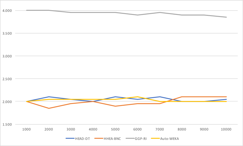
As mentioned earlier, the analysis of the results so far focused only on the runtime limits of 1,000s and 10,000s due to space restrictions, but we performed experiments with 10 different limits (from 1,000s up to 10,000s). Figure 2(a) shows the evolution of the GMean average ranks for the four meta-learning methods across the 10 runtime limits. This figure shows that HHEA-BNC tends to achieve overall the best (lowest) average rank until the runtime limit of 7,000s, whilst for longer runtime limits Auto-WEKA and HEAD-DT tend to share the best rank, with Auto-WEKA slightly better at the last runtime limit.

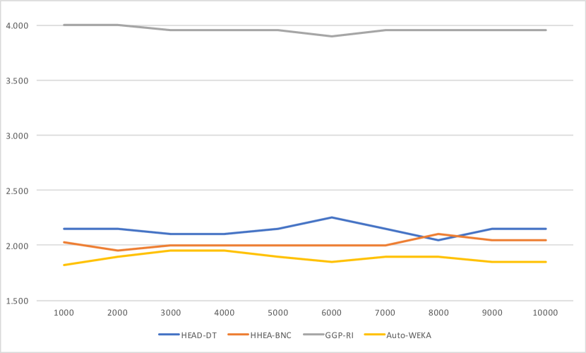
Figure 2(b) shows the same evolution, but this time regarding average accuracy ranks. In this case, Auto-WEKA remains the best method across all runtime limits, and for nearly all runtime limits, the second place is obtained by HHEA-BNC. Note that GGP-RI remained consistently the worst method across all 10 runtime limits, for both GMean and accuracy results.

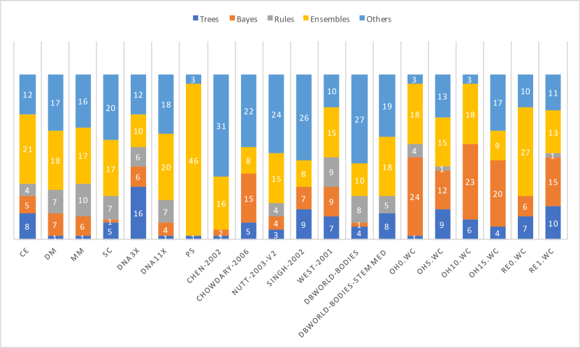
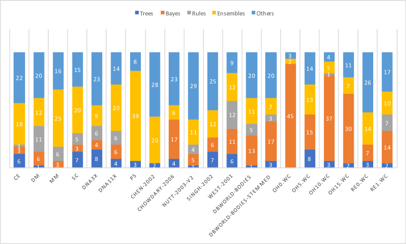
Figures 3(a) and 3(b) show the broad types of algorithms recommended by Auto-WEKA per dataset, for the runtime limits of 1,000s and 10,000s, respectively. Since Auto-WEKA considers a large number of algorithms, instead of referring to specific algorithms, the graphs show the frequency of recommendations for five broad types of algorithms, namely: the three types of algorithms that are considered by the three EAs (decision trees, if-then classification rules, and Bayesian network classifiers), ensemble methods and all the others. Note that the variability of the selected types of algorithms is high, highlighting the difficulty of selecting the best algorithm for each dataset.

For the runtime limit of 1,000s (Figure 3(a)), ensembles had the highest prevalence across the datasets; they were selected by Auto-WEKA in 33.9% of the cases, closely followed by decision-tree algorithms, selected in 31.4% of the cases. For the runtime limit of 10,000s (Figure 3(b)), these two types of classification algorithms swapped places in the ranking by prevalence, i.e., decision-tree algorithms were selected by Auto-WEKA in 34.7% of the cases, whilst ensembles were selected in 27.3% of the cases. Bayesian classification algorithms also did relatively well, partly because they had a high prevalence among the text mining datasets. For both runtime limits, Bayesian classification algorithms were the third most selected type of classification algorithm: they were selected in 16.7% of the cases in Figure 3(a) and in 24.2% of the cases in Figure 3(b). For both runtime limits, rule induction algorithms had small frequencies of selection, only 7.9% in Figure 3(a) and 6.7% in Figure 3(b). This is consistent with the fact that, out of the 3 EAs for AutoML evaluated in this work, GGP-RI (which evolved rule induction algorithms) obtained clearly the worst result.

4.2 More extensive experiments comparing HEAD-DT and Auto-WEKA

In this section we compare HEAD-DT and Auto-WEKA in an extended set of 40 datasets. This includes the 20 datasets used in the previous section plus 20 other datasets, as discussed in Section 3.1. As mentioned earlier, the motivation for using this larger set of datasets only to compare the two methods in this section, rather than to compare more methods in the previous section, is the much larger amount of time associated with the experiments using all the 40 datasets. This section uses the same experimental methodology used in the previous section, using 10-fold cross-validation and comparing the two methods with the same runtime limit, varying this limit from 1,000s to 10,000s, in increments of 1,000s. Again, due to space restrictions, we report results only for the smallest and longest runtime limits, namely 1,000s and 10,000s; but the results for the 10 different runtime limits can be found in the Supplementary Results file.

Table 9: Accuracy results for HEAD-DT and Auto-WEKA (time limits: 1,000s and 10,000s).

	1,000s		10,000s
	HEAD-DT	Auto-WEKA	HEAD-DT	Auto-WEKA
CE	0.613	0.649	0.623	0.649
DM	0.637	0.672	0.604	0.665
MM	0.720	0.722	0.702	0.706
SC	0.826	0.828	0.818	0.826
DNA3	0.846	0.856	0.847	0.855
DNA11	0.752	0.708	0.747	0.701
PS	0.982	0.975	0.984	0.975
chen-2002	0.896	0.926	0.896	0.927
chowdary-2006	0.959	0.991	0.959	0.993
nutt-2003-v2	0.760	0.840	0.760	0.873
singh-2002	0.772	0.867	0.772	0.877
west-2001	0.910	0.880	0.910	0.868
dbworld-bodies	0.721	0.764	0.721	0.812
dbworld-bodies-stemmed	0.806	0.825	0.806	0.891
oh0.wc	0.825	0.778	0.824	0.809
oh5.wc	0.846	0.789	0.850	0.793
oh10.wc	0.777	0.721	0.773	0.727
oh15.wc	0.746	0.774	0.764	0.778
re0.wc	0.755	0.783	0.752	0.774
re1.wc	0.807	0.755	0.820	0.767
abalone	0.265	0.263	0.269	0.263
car	0.984	0.994	0.983	0.997
convex	0.712	0.531	0.714	0.531
germancredit	0.750	0.738	0.750	0.739
krvskp	0.995	0.962	0.995	0.962
madelon	0.781	0.735	0.768	0.784
mnist	0.886	0.929	0.887	0.934
mnistrotationbackimagenew	0.343	0.214	0.343	0.225
secom	0.932	0.932	0.931	0.933
semeion	0.763	0.894	0.758	0.907
shuttle	1.000	0.999	1.000	0.999
waveform	0.760	0.868	0.763	0.868
winequalitywhite	0.622	0.676	0.627	0.672
yeast	0.584	0.602	0.582	0.607
sick	0.989	0.978	0.989	0.980
splice	0.990	0.949	0.988	0.955
kropt	0.796	0.680	0.801	0.761
quake	0.535	0.553	0.529	0.546
pc4	0.889	0.891	0.886	0.896
magicTelescope	0.852	0.831	0.853	0.840
Average	0.785	0.783	0.784	0.792
# wins	18	21	17	23

Table 10: GMean results for HEAD-DT and Auto-WEKA (time limits: 1,000s and 10,000s).

	1,000s		10,000s
	HEAD-DT	Auto-WEKA	HEAD-DT	Auto-WEKA
CE	0.564	0.604	0.581	0.605
DM	0.559	0.557	0.517	0.544
MM	0.596	0.572	0.590	0.563
SC	0.535	0.471	0.559	0.454
DNA3	0.704	0.700	0.705	0.712
DNA11	0.568	0.506	0.578	0.524
PS	0.888	0.830	0.897	0.838
chen-2002	0.891	0.922	0.892	0.925
chowdary-2006	0.956	0.988	0.956	0.991
nutt-2003-v2	0.790	0.861	0.790	0.887
singh-2002	0.772	0.867	0.772	0.877
west-2001	0.913	0.888	0.913	0.878
dbworld-bodies	0.725	0.765	0.725	0.816
dbworld-bodies-stemmed	0.815	0.825	0.815	0.892
oh0.wc	0.895	0.863	0.893	0.884
oh5.wc	0.911	0.878	0.914	0.880
oh10.wc	0.867	0.831	0.864	0.835
oh15.wc	0.847	0.864	0.859	0.867
re0.wc	0.831	0.849	0.831	0.841
re1.wc	0.886	0.851	0.894	0.859
abalone	0.486	0.483	0.489	0.483
car	0.987	0.996	0.987	0.998
convex	0.712	0.531	0.714	0.531
germancredit	0.655	0.630	0.657	0.638
krvskp	0.995	0.961	0.995	0.962
madelon	0.781	0.735	0.768	0.784
mnist	0.935	0.960	0.936	0.963
mnistrotationbackimagenew	0.564	0.441	0.564	0.452
secom	0.254	0.274	0.256	0.268
semeion	0.862	0.940	0.859	0.947
shuttle	1.000	0.997	1.000	0.997
waveform	0.818	0.900	0.820	0.900
winequalitywhite	0.712	0.738	0.716	0.728
yeast	0.708	0.721	0.706	0.724
sick	0.940	0.888	0.943	0.894
splice	0.993	0.961	0.991	0.965
kropt	0.881	0.808	0.884	0.858
quake	0.516	0.498	0.506	0.496
pc4	0.689	0.550	0.694	0.579
magicTelescope	0.821	0.793	0.823	0.802
Average	0.770	0.757	0.771	0.766
# wins	24	16	21	19

Table 9 and Table 10 show the accuracy and GMean values, respectively, obtained by HEAD-DT and Auto-WEKA with the runtime limits of 1,000s and 10,000s. In terms of accuracy, Auto-WEKA has somewhat outperformed HEAD-DT overall, whilst the opposite was observed for the GMean measure. This result is consistent with the fact that Auto-WEKA’s search tries to optimize the accuracy measure (unlike HEAD-DT), as discussed earlier. However, the result of a Wilcoxon significance test, at the conventional significance level of 0.05, indicates that there is no statistically significant difference of predictive performance between HEAD-DT and Auto-WEKA (for both accuracy and GMean measures), for each of the 10 runtime limits.

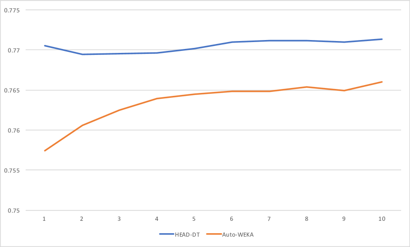
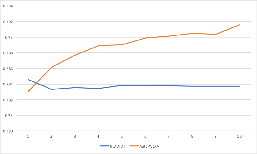
Figure 4(a) shows the evolution of the average GMean values (across all datasets) for Auto-WEKA and HEAD-DT across the 10 runtime limits. This figure shows that HEAD-DT obtains a better (higher) GMean value for all runtime limits. Figure 4(b) shows the same type of evolution for the accuracy measure. In this case, HEAD-DT obtains the best average accuracy for the smallest runtime limit, but Auto-WEKA obtains higher accuracy for all other runtime limits. It should be noted, however, that in both graphs the differences of predictive performance between HEAD-DT and Auto-WEKA are small, less than 1% in general, across the different runtime limits.

Finally, the presence of signs of overfitting for HEAD-DT and Auto-WEKA was also investigated. This investigation compared HEAD-DT’s GMean values on the validation set (a holdout part of the training set) and Auto-WEKA-Trees’ GMean values for the internal 10-CV procedure (on the training set) with their corresponding GMean values on the test set. A GMean value on the test set much smaller than the corresponding GMean value on the validation set or internal 10-CV procedure (depending on the method) was considered a sign of overfitting. This kind of overfitting can be called meta-overfitting, since it occurs at the meta-learning level, rather than the conventional overfitting at the base-learning level (involving the difference between GMean values on the training and validation sets).

Note that the meta-overfitting is measured in somewhat different ways in HEAD-DT and Auto- WEKA due to the different approaches to evaluate candidate solutions during their searches. That is, HEAD-DT performs a single partition of the training set into two subsets, one for building the model, the other (validation set) for evaluating the model; whilst Auto-WEKA uses internal cross-validation on the training set. Despite this difference, the principle used for measuring meta-overfitting is the same in both types of methods: the degree of meta-overfitting is measured by comparing predictive performance on the test set (not accessed during the entire execution of HEAD-DT or Auto-WEKA) with the predictive performance on the part of the training set used as a hold-out set to evaluate the model built from the remaining part of the training set.

For the runtime limit of 1,000s (10,000s), the average GMean value (over all 40 datasets) of HEAD-DT on the validation set is 0.756 (0.758), whilst its average GMean on the test set is 0.770 (0.771). In addition, for the runtime limit of 1,000s (10,000s), the average accuracy value of HEAD-DT on the validation set is 0.766 (0.767), whilst its average accuracy on the test set is 0.785 and 0.784. Hence, HEAD-DT shows no sign of meta-overfitting, since its GMean and accuracy values on the test set are slightly larger than on the validation set. This small increase in the GMean and accuracy values on the test set, for both runtime limits, can be explained mainly by two factors. First, since the algorithms were evolved by HEAD-DT using the F-measure of precision and recall in the fitness function, they were not optimizing GMean or accuracy. Second, the classifier used to classify the test set is in principle a higher-quality classifier than the one used to classify the validation set, because the former was induced from all training instances, whilst the latter was induced from a subset of the training set (excluding the validation set).

Turning to Auto-WEKA, for the runtime limit of 1,000s (10,000s), the average GMean value (over all 40 datasets) for the internal 10-CV of Auto-WEKA is 0.896 (0.899), whilst its GMean on the test set is 0.757 (0.766). In addition, for the runtime limit of 1,000s (10,000s), the average accuracy value for the internal 10-CV of Auto-WEKA is 0.912 (0.915), whilst its accuracy on the test set is 0.783 (0.792). Hence, for both the GMean and accuracy measures, Auto-WEKA clearly shows a substantial degree of meta-overfitting.

5 Conclusions

AutoML is currently a very popular issue, having attracted a great deal of attention, with the proposal of new tools, mainly based on optimization [Hutter et al., 2019, Elsken et al., 2019, Mohr et al., 2018, das Dôres et al., 2018, Li et al., 2018, Larcher and Barbosa, 2019, Koch et al., 2018, Jin et al., 2019, Fusi et al., 2018]. Based on the relevance of AutoML, this work has evaluated four methods for recommending a classification algorithm for a target dataset: three Evolutionary Algorithms (EAs) and Auto-WEKA [Thornton et al., 2013], in two sets of experiments. In the first set of experiments, we have compared the four AutoML methods with the same runtime limit on 20 datasets. Auto-WEKA can recommend classification algorithms of various types (paradigms), whilst each of the three EAs is restricted to recommend a different type of classification algorithm: decision tree, rule induction or Bayesian network classification algorithms, in the case of HEAD-DT, GGP-RI and HHEA-BNC, respectively. In these experiments, there was no statistically significant difference of predictive accuracy between the three best methods, namely two EAs (HEAD-DT and HHEA-BNC) and Auto-WEKA. However, these three methods obtained significantly better predictive accuracy than the other EA (GGP-RI). These results were broadly consistent across the 10 different runtime limits used in the experiments. In the second set of experiments, where a larger set of 40 datasets was used to compare the predictive accuracy of HEAD-DT and Auto-WEKA only, again there was no statistically significant difference between the predictive performance of these two methods.

However, the focus of HEAD-DT on only on decision-tree algorithms has two advantages from the perspective of other algorithm-evaluation criteria. First, in applications where it is important that the classification model be interpreted by users (e.g. in medical applications), decision-tree algorithms have the advantage of generating interpretable classification models. By contrast, since Auto-WEKA can select any algorithm out of many types of classification algorithm, it can recommend classification algorithms producing black-box (non-interpretable) models. Indeed, in our experiments, Auto-WEKA often recommended ensembles, which are not easily interpretable. Second, decision-tree algorithms also have the advantage of being in general more scalable to large datasets than several other types of classification algorithms in Auto-WEKA’s search space, like neural networks, support vector machines and some ensemble methods.

Overall, when the runtime limit is increased from 1,000s to 10,000s, Auto-WEKA benefits more from the extra search time than HEAD-DT. This seems due to the fact that Auto-WEKA has to explore a much more diverse space of classification algorithms, so it probably requires more time to find the best type of classification algorithm to be recommended for a given input dataset.

In addition, we observed that Auto-WEKA exhibited meta-overfitting, where the GMean values on the training set were substantially lower than the GMean values on the test set, for the best algorithm found by Auto-WEKA. As noted earlier, this meta-overfitting is a form of overfitting at the meta-learning level, due to evaluating many different (base-level) classification algorithms during Auto-WEKA’s search for the best algorithm. This is in contrast to the standard overfitting at the base level, due to evaluating many different models built by the same classification algorithm.

5.1 Future Work

It would be interesting to enhance the search process of the EAs by first performing a global search to optimise the candidate algorithms’ (procedural) components, followed by a second (global or local) search to optimise the continuous parameters of the best algorithm generated by the first search. Another future research direction is to extend the EAs to produce an ensemble of evolved classification algorithms in a post-processing phase, after the EAs have completed their search.

Besides, since Auto-WEKA showed a clear sign of meta-overfitting, another research direction consists of developing new meta-overfitting-avoidance methods that could potentially improve the predictive performance of Auto-WEKA. Finally, it would be interesting to compare the three EAs and Auto-WEKA to other AutoML methods, such as Auto-sklearn and those described in Section 2.2.4. This would give us a more detailed assessment about which AutoML method recommends the best classification algorithm, taking into account different datasets.

Appendix A Supplementary Material for: An Extensive Experimental Evaluation of Automated Machine Learning Methods for Recommending Classification Algorithms

Table A1: Results of predictive Specificity values of the baseline methods for building decision tree models.

data set	Decision Stump	J48	LMT	RandomTrees	REPTree
CE	0.499	0.585	0.576	0.496	0.541
DM	0.348	0.545	0.423	0.449	0.315
MM	0.312	0.496	0.403	0.484	0.292
SC	0.280	0.542	0.362	0.412	0.297
DNA3	0.562	0.720	0.604	0.482	0.562
DNA11	0.260	0.478	0.420	0.491	0.288
PS	0.700	0.801	0.794	0.913	0.823
chen-2002	0.857	0.798	0.944	0.826	0.756
chowdary-2006	0.965	0.951	0.969	0.918	0.930
nutt-2003-v2	0.933	0.933	0.850	0.733	0.600
singh-2002	0.746	0.781	0.901	0.754	0.696
west-2001	0.862	0.815	0.878	0.578	0.782
dbworld-bodies	0.770	0.743	0.819	0.686	0.758
dbworld-bodies-stemmed	0.900	0.792	0.758	0.596	0.811
oh0.wc	0.857	0.972	0.979	0.925	0.962
oh5.wc	0.857	0.976	0.985	0.921	0.975
oh10.wc	0.863	0.961	0.967	0.921	0.962
oh15.wc	0.851	0.966	0.973	0.921	0.952
re0.wc	0.736	0.915	0.940	0.881	0.909
re1.wc	0.829	0.970	0.979	0.941	0.970
Average	0.699	0.787	0.776	0.716	0.709

Table A2: Results of predictive Sensitivity values of the baseline methods for building decision tree models.

data set	Decision Stump	J48	LMT	RandomTrees	REPTree
CE	0.623	0.648	0.659	0.567	0.642
DM	0.614	0.664	0.623	0.555	0.623
MM	0.631	0.661	0.640	0.631	0.708
SC	0.827	0.822	0.835	0.774	0.807
DNA3	0.863	0.841	0.848	0.733	0.863
DNA11	0.720	0.777	0.740	0.706	0.726
PS	0.981	0.985	0.985	0.985	0.983
chen-2002	0.821	0.810	0.949	0.827	0.787
chowdary-2006	0.971	0.951	0.972	0.923	0.944
nutt-2003-v2	0.867	0.867	0.850	0.717	0.450
singh-2002	0.744	0.783	0.903	0.756	0.694
west-2001	0.855	0.835	0.855	0.555	0.735
dbworld-bodies	0.738	0.740	0.814	0.698	0.733
dbworld-bodies-stemmed	0.867	0.783	0.767	0.612	0.798
oh0.wc	0.351	0.820	0.874	0.463	0.779
oh5.wc	0.261	0.807	0.883	0.356	0.805
oh10.wc	0.262	0.727	0.754	0.368	0.742
oh15.wc	0.272	0.736	0.810	0.387	0.653
re0.wc	0.537	0.745	0.832	0.559	0.739
re1.wc	0.396	0.798	0.859	0.472	0.786
Average	0.660	0.790	0.823	0.632	0.750

Table A3: Results of predictive GMean values of the baseline methods for building decision tree models.

data set	Decision Stump	J48	LMT	RandomTrees	REPTree
CE	0.557	0.616	0.616	0.530	0.589
DM	0.460	0.600	0.511	0.496	0.442
MM	0.435	0.569	0.499	0.537	0.451
SC	0.464	0.663	0.535	0.556	0.466
DNA3	0.694	0.773	0.707	0.584	0.694
DNA11	0.426	0.601	0.553	0.586	0.450
PS	0.828	0.888	0.884	0.948	0.899
chen-2002	0.838	0.804	0.947	0.826	0.771
chowdary-2006	0.968	0.951	0.970	0.920	0.937
nutt-2003-v2	0.898	0.898	0.846	0.721	0.507
singh-2002	0.745	0.782	0.902	0.755	0.695
west-2001	0.858	0.823	0.866	0.563	0.756
dbworld-bodies	0.753	0.741	0.816	0.691	0.745
dbworld-bodies-stemmed	0.883	0.787	0.762	0.603	0.804
oh0.wc	0.548	0.892	0.925	0.654	0.865
oh5.wc	0.473	0.887	0.933	0.568	0.886
oh10.wc	0.475	0.835	0.854	0.581	0.844
oh15.wc	0.480	0.842	0.888	0.595	0.788
re0.wc	0.629	0.826	0.884	0.702	0.820
re1.wc	0.573	0.880	0.917	0.666	0.873
Average	0.649	0.783	0.791	0.654	0.714

Table A4: Results of predictive Specificity values of HEAD-DT for timeouts from 1,000s to 5,000s.

data set	1,000s	2,000s	3,000s	4,000s	5,000s
CE	0.693	0.664	0.656	0.691	0.676
DM	0.808	0.758	0.758	0.758	0.825
MM	0.733	0.739	0.739	0.739	0.675
SC	0.767	0.724	0.701	0.701	0.701
DNA3	0.846	0.846	0.846	0.846	0.846
DNA11	0.854	0.833	0.833	0.833	0.833
PS	0.978	0.989	0.989	0.975	0.978
chen-2002	0.964	0.937	0.937	0.937	0.937
chowdary-2006	0.965	0.965	0.965	0.965	0.965
nutt-2003-v2	0.983	0.983	0.983	0.983	0.983
singh-2002	0.852	0.852	0.852	0.852	0.852
west-2001	0.973	0.973	0.973	0.973	0.973
dbworld-bodies	0.844	0.844	0.844	0.844	0.844
dbworld-bodies-stemmed	0.846	0.846	0.846	0.846	0.846
oh0.wc	0.984	0.984	0.981	0.980	0.980
oh5.wc	0.991	0.991	0.990	0.991	0.990
oh10.wc	0.975	0.975	0.975	0.975	0.979
oh15.wc	0.977	0.978	0.979	0.980	0.980
re0.wc	0.961	0.952	0.953	0.954	0.955
re1.wc	0.986	0.985	0.985	0.983	0.983
Average	0.899	0.891	0.889	0.890	0.890

Table A5: Results of predictive Specificity values of HEAD-DT for timeouts from 6,000s to 10,000s.

data set	6,000s	7,000s	8,000s	9,000s	10,000s
CE	0.676	0.676	0.682	0.708	0.708
DM	0.825	0.796	0.796	0.796	0.796
MM	0.675	0.675	0.675	0.675	0.675
SC	0.701	0.701	0.722	0.722	0.722
DNA3	0.846	0.846	0.846	0.846	0.846
DNA11	0.833	0.807	0.807	0.807	0.807
PS	0.978	0.978	0.978	0.978	0.978
chen-2002	0.937	0.937	0.937	0.937	0.937
chowdary-2006	0.965	0.965	0.965	0.965	0.965
nutt-2003-v2	0.983	0.983	0.983	0.983	0.983
singh-2002	0.852	0.852	0.852	0.852	0.852
west-2001	0.973	0.973	0.973	0.973	0.973
dbworld-bodies	0.844	0.844	0.844	0.844	0.844
dbworld-bodies-stemmed	0.846	0.846	0.846	0.846	0.846
oh0.wc	0.981	0.982	0.982	0.982	0.982
oh5.wc	0.990	0.990	0.990	0.990	0.990
oh10.wc	0.979	0.979	0.980	0.980	0.980
oh15.wc	0.982	0.982	0.982	0.982	0.982
re0.wc	0.954	0.957	0.957	0.957	0.957
re1.wc	0.984	0.984	0.985	0.985	0.985
Average	0.890	0.888	0.889	0.890	0.890

Table A6: Results of predictive Sensitivity values of HEAD-DT for timeouts from 1,000s to 5,000s.

data set	1,000s	2,000s	3,000s	4,000s	5,000s
CE	0.759	0.749	0.736	0.759	0.751
DM	0.867	0.842	0.842	0.842	0.875
MM	0.867	0.878	0.878	0.878	0.875
SC	0.943	0.927	0.915	0.915	0.915
DNA3	0.935	0.935	0.935	0.935	0.935
DNA11	0.933	0.919	0.919	0.919	0.919
PS	0.998	0.999	0.999	0.998	0.998
chen-2002	0.966	0.950	0.950	0.950	0.950
chowdary-2006	0.971	0.971	0.971	0.971	0.971
nutt-2003-v2	0.967	0.967	0.967	0.967	0.967
singh-2002	0.851	0.851	0.851	0.851	0.851
west-2001	0.960	0.960	0.960	0.960	0.960
dbworld-bodies	0.831	0.831	0.831	0.831	0.831
dbworld-bodies-stemmed	0.829	0.829	0.829	0.829	0.829
oh0.wc	0.896	0.901	0.887	0.884	0.884
oh5.wc	0.930	0.925	0.922	0.922	0.917
oh10.wc	0.834	0.839	0.840	0.837	0.855
oh15.wc	0.845	0.851	0.855	0.858	0.859
re0.wc	0.888	0.870	0.874	0.878	0.878
re1.wc	0.893	0.893	0.887	0.874	0.879
Average	0.898	0.894	0.892	0.893	0.895

Table A7: Results of predictive Sensitivity values of HEAD-DT for timeouts from 6,000s to 10,000s.

data set	6,000s	7,000s	8,000s	9,000s	10,000s
CE	0.751	0.751	0.764	0.779	0.779
DM	0.875	0.867	0.867	0.867	0.867
MM	0.875	0.875	0.875	0.875	0.875
SC	0.915	0.911	0.919	0.919	0.915
DNA3	0.935	0.935	0.935	0.935	0.935
DNA11	0.919	0.911	0.911	0.911	0.911
PS	0.998	0.998	0.998	0.998	0.998
chen-2002	0.950	0.950	0.950	0.950	0.950
chowdary-2006	0.971	0.971	0.971	0.971	0.971
nutt-2003-v2	0.967	0.967	0.967	0.967	0.967
singh-2002	0.851	0.851	0.851	0.851	0.851
west-2001	0.960	0.960	0.960	0.960	0.960
dbworld-bodies	0.831	0.831	0.831	0.831	0.831
dbworld-bodies-stemmed	0.829	0.829	0.829	0.829	0.829
oh0.wc	0.886	0.892	0.892	0.892	0.892
oh5.wc	0.912	0.912	0.912	0.912	0.916
oh10.wc	0.855	0.855	0.858	0.858	0.858
oh15.wc	0.865	0.865	0.874	0.872	0.872
re0.wc	0.875	0.880	0.880	0.880	0.880
re1.wc	0.883	0.891	0.893	0.893	0.893
Average	0.895	0.895	0.897	0.897	0.897

Table A8: Results of predictive GMean values of HEAD-DT for timeouts from 1,000s to 5,000s.

data set	1,000s	2,000s	3,000s	4,000s	5,000s
CE	0.725	0.705	0.694	0.724	0.712
DM	0.834	0.794	0.794	0.794	0.846
MM	0.789	0.797	0.797	0.797	0.756
SC	0.846	0.806	0.788	0.788	0.788
DNA3	0.887	0.887	0.887	0.887	0.887
DNA11	0.890	0.873	0.873	0.873	0.873
PS	0.988	0.994	0.994	0.986	0.988
chen-2002	0.965	0.943	0.943	0.943	0.943
chowdary-2006	0.968	0.968	0.968	0.968	0.968
nutt-2003-v2	0.975	0.975	0.975	0.975	0.975
singh-2002	0.852	0.852	0.852	0.852	0.852
west-2001	0.967	0.967	0.967	0.967	0.967
dbworld-bodies	0.837	0.837	0.837	0.837	0.837
dbworld-bodies-stemmed	0.837	0.837	0.837	0.837	0.837
oh0.wc	0.939	0.941	0.933	0.931	0.931
oh5.wc	0.960	0.957	0.955	0.955	0.953
oh10.wc	0.901	0.904	0.904	0.902	0.915
oh15.wc	0.909	0.912	0.915	0.916	0.917
re0.wc	0.924	0.910	0.913	0.915	0.916
re1.wc	0.938	0.938	0.934	0.927	0.929
Average	0.896	0.890	0.888	0.889	0.889

Table A9: Results of predictive GMean values of HEAD-DT for timeouts from 6,000s to 10,000s.

data set	6,000s	7,000s	8,000s	9,000s	10,000s
CE	0.712	0.712	0.721	0.742	0.742
DM	0.846	0.827	0.827	0.827	0.827
MM	0.756	0.756	0.756	0.756	0.756
SC	0.788	0.786	0.803	0.803	0.801
DNA3	0.887	0.887	0.887	0.887	0.887
DNA11	0.873	0.855	0.855	0.855	0.855
PS	0.988	0.988	0.988	0.988	0.988
chen-2002	0.943	0.943	0.943	0.943	0.943
chowdary-2006	0.968	0.968	0.968	0.968	0.968
nutt-2003-v2	0.975	0.975	0.975	0.975	0.975
singh-2002	0.852	0.852	0.852	0.852	0.852
west-2001	0.967	0.967	0.967	0.967	0.967
dbworld-bodies	0.837	0.837	0.837	0.837	0.837
dbworld-bodies-stemmed	0.837	0.837	0.837	0.837	0.837
oh0.wc	0.932	0.936	0.936	0.936	0.936
oh5.wc	0.950	0.950	0.950	0.950	0.952
oh10.wc	0.915	0.915	0.917	0.917	0.917
oh15.wc	0.921	0.921	0.926	0.925	0.925
re0.wc	0.913	0.917	0.917	0.917	0.917
re1.wc	0.932	0.936	0.938	0.938	0.938
Average	0.890	0.888	0.890	0.891	0.891

Table A10: Results of predictive Specificity values of Auto-WEKA-Trees for timeouts from 1,000s to 5,000s.

data set	1,000s	2,000s	3,000s	4,000s	5,000s
CE	0.539	0.547	0.549	0.552	0.552
DM	0.378	0.363	0.361	0.366	0.388
MM	0.399	0.418	0.417	0.418	0.418
SC	0.254	0.253	0.253	0.259	0.254
DNA3	0.554	0.593	0.578	0.589	0.612
DNA11	0.403	0.376	0.401	0.377	0.362
PS	0.699	0.702	0.711	0.721	0.722
chen-2002	0.924	0.926	0.914	0.917	0.918
chowdary-2006	0.993	0.994	0.994	0.994	0.993
nutt-2003-v2	0.879	0.854	0.854	0.854	0.854
singh-2002	0.892	0.886	0.886	0.881	0.875
west-2001	0.914	0.914	0.914	0.914	0.914
dbworld-bodies	0.738	0.743	0.734	0.738	0.763
dbworld-bodies-stemmed	0.863	0.843	0.793	0.769	0.771
oh0.wc	0.965	0.965	0.966	0.966	0.966
oh5.wc	0.981	0.981	0.980	0.980	0.980
oh10.wc	0.959	0.959	0.959	0.958	0.959
oh15.wc	0.967	0.967	0.968	0.968	0.969
re0.wc	0.921	0.919	0.920	0.920	0.920
re1.wc	0.968	0.968	0.969	0.969	0.969
Average	0.759	0.759	0.756	0.756	0.758

Table A11: Results of predictive Specificity values of Auto-WEKA-Trees for timeouts from 6,000s to 10,000s.

data set	6,000s	7,000s	8,000s	9,000s	10,000s
CE	0.553	0.558	0.553	0.555	0.558
DM	0.387	0.389	0.388	0.375	0.387
MM	0.418	0.414	0.413	0.416	0.402
SC	0.259	0.254	0.290	0.258	0.269
DNA3	0.600	0.610	0.598	0.608	0.601
DNA11	0.388	0.379	0.378	0.422	0.387
PS	0.723	0.744	0.736	0.748	0.747
chen-2002	0.920	0.923	0.915	0.914	0.912
chowdary-2006	0.993	0.993	0.993	0.993	0.988
nutt-2003-v2	0.858	0.858	0.850	0.854	0.875
singh-2002	0.872	0.875	0.872	0.872	0.877
west-2001	0.914	0.908	0.908	0.908	0.908
dbworld-bodies	0.737	0.739	0.739	0.739	0.739
dbworld-bodies-stemmed	0.769	0.769	0.772	0.772	0.772
oh0.wc	0.966	0.966	0.966	0.966	0.966
oh5.wc	0.981	0.980	0.980	0.980	0.980
oh10.wc	0.958	0.959	0.958	0.959	0.958
oh15.wc	0.969	0.969	0.969	0.969	0.969
re0.wc	0.920	0.919	0.917	0.917	0.917
re1.wc	0.969	0.969	0.969	0.969	0.969
Average	0.758	0.759	0.758	0.760	0.759

Table A12: Results of predictive Sensitivity values of Auto-WEKA-Trees for timeouts from 1,000s to 5,000s.

data set	1,000s	2,000s	3,000s	4,000s	5,000s
CE	0.635	0.643	0.644	0.645	0.645
DM	0.634	0.628	0.630	0.628	0.641
MM	0.683	0.692	0.686	0.692	0.692
SC	0.820	0.817	0.817	0.818	0.820
DNA3	0.833	0.847	0.831	0.834	0.843
DNA11	0.704	0.715	0.720	0.706	0.708
PS	0.976	0.976	0.976	0.977	0.977
chen-2002	0.931	0.934	0.926	0.927	0.927
chowdary-2006	0.991	0.993	0.993	0.993	0.991
nutt-2003-v2	0.821	0.796	0.796	0.796	0.796
singh-2002	0.893	0.889	0.889	0.884	0.877
west-2001	0.899	0.899	0.899	0.899	0.899
dbworld-bodies	0.748	0.747	0.739	0.745	0.770
dbworld-bodies-stemmed	0.848	0.830	0.786	0.770	0.770
oh0.wc	0.802	0.804	0.808	0.810	0.809
oh5.wc	0.807	0.807	0.805	0.807	0.807
oh10.wc	0.725	0.721	0.726	0.721	0.724
oh15.wc	0.775	0.778	0.783	0.783	0.788
re0.wc	0.745	0.768	0.770	0.769	0.768
re1.wc	0.766	0.766	0.767	0.767	0.768
Average	0.802	0.803	0.800	0.799	0.801

Table A13: Results of predictive Sensitivity values of Auto-WEKA-Trees for timeouts from 6,000s to 10,000s.

data set	6,000s	7,000s	8,000s	9,000s	10,000s
CE	0.645	0.648	0.645	0.646	0.648
DM	0.645	0.642	0.640	0.641	0.660
MM	0.692	0.692	0.689	0.686	0.683
SC	0.818	0.820	0.825	0.817	0.818
DNA3	0.842	0.843	0.843	0.838	0.834
DNA11	0.712	0.711	0.717	0.721	0.715
PS	0.977	0.978	0.978	0.979	0.978
chen-2002	0.930	0.931	0.926	0.926	0.926
chowdary-2006	0.991	0.991	0.991	0.991	0.983
nutt-2003-v2	0.804	0.804	0.788	0.796	0.813
singh-2002	0.874	0.877	0.874	0.874	0.879
west-2001	0.899	0.893	0.893	0.893	0.893
dbworld-bodies	0.754	0.755	0.755	0.755	0.755
dbworld-bodies-stemmed	0.766	0.766	0.770	0.770	0.770
oh0.wc	0.810	0.810	0.810	0.805	0.806
oh5.wc	0.810	0.808	0.808	0.808	0.810
oh10.wc	0.721	0.723	0.727	0.728	0.722
oh15.wc	0.790	0.791	0.792	0.791	0.792
re0.wc	0.769	0.768	0.768	0.767	0.770
re1.wc	0.768	0.768	0.768	0.767	0.769
Average	0.801	0.801	0.800	0.800	0.801

Table A14: Results of predictive GMean values of Auto-WEKA-Trees for timeouts from 1,000s to 5,000s.

data set	1,000s	2,000s	3,000s	4,000s	5,000s
CE	0.539	0.547	0.549	0.552	0.552
DM	0.378	0.363	0.361	0.366	0.388
MM	0.399	0.418	0.417	0.418	0.418
SC	0.254	0.253	0.253	0.259	0.254
DNA3	0.554	0.593	0.578	0.589	0.612
DNA11	0.403	0.376	0.401	0.377	0.362
PS	0.699	0.702	0.711	0.721	0.722
chen-2002	0.924	0.926	0.914	0.917	0.918
chowdary-2006	0.993	0.994	0.994	0.994	0.993
nutt-2003-v2	0.879	0.854	0.854	0.854	0.854
singh-2002	0.892	0.886	0.886	0.881	0.875
west-2001	0.914	0.914	0.914	0.914	0.914
dbworld-bodies	0.738	0.743	0.734	0.738	0.763
dbworld-bodies-stemmed	0.863	0.843	0.793	0.769	0.771
oh0.wc	0.965	0.965	0.966	0.966	0.966
oh5.wc	0.981	0.981	0.980	0.980	0.980
oh10.wc	0.959	0.959	0.959	0.958	0.959
oh15.wc	0.967	0.967	0.968	0.968	0.969
re0.wc	0.921	0.919	0.920	0.920	0.920
re1.wc	0.968	0.968	0.969	0.969	0.969
Average	0.759	0.759	0.756	0.756	0.758

Table A15: Results of predictive GMean values of Auto-WEKA-Trees for timeouts from 6,000s to 10,000s.

data set	6,000s	7,000s	8,000s	9,000s	10,000s
CE	0.553	0.558	0.553	0.555	0.558
DM	0.387	0.389	0.388	0.375	0.387
MM	0.418	0.414	0.413	0.416	0.402
SC	0.259	0.254	0.290	0.258	0.269
DNA3	0.600	0.610	0.598	0.608	0.601
DNA11	0.388	0.379	0.378	0.422	0.387
PS	0.723	0.744	0.736	0.748	0.747
chen-2002	0.920	0.923	0.915	0.914	0.912
chowdary-2006	0.993	0.993	0.993	0.993	0.988
nutt-2003-v2	0.858	0.858	0.850	0.854	0.875
singh-2002	0.872	0.875	0.872	0.872	0.877
west-2001	0.914	0.908	0.908	0.908	0.908
dbworld-bodies	0.737	0.739	0.739	0.739	0.739
dbworld-bodies-stemmed	0.769	0.769	0.772	0.772	0.772
oh0.wc	0.966	0.966	0.966	0.966	0.966
oh5.wc	0.981	0.980	0.980	0.980	0.980
oh10.wc	0.958	0.959	0.958	0.959	0.958
oh15.wc	0.969	0.969	0.969	0.969	0.969
re0.wc	0.920	0.919	0.917	0.917	0.917
re1.wc	0.969	0.969	0.969	0.969	0.969
Average	0.758	0.759	0.758	0.760	0.759

Table A16: Results of predictive Specificity values of the baseline methods for inducing rule-based models.

data set	Decision Table	JRip	OneR	PART	ZeroR
CE	0.537	0.565	0.571	0.550	0.398
DM	0.416	0.456	0.382	0.511	0.327
MM	0.480	0.430	0.494	0.534	0.292
SC	0.345	0.378	0.221	0.458	0.161
DNA3	0.506	0.606	0.513	0.641	0.237
DNA11	0.284	0.373	0.370	0.565	0.244
PS	0.761	0.852	0.700	0.884	0.060
chen-2002	0.854	0.790	0.778	0.858	0.419
chowdary-2006	0.935	0.954	0.965	0.936	0.404
nutt-2003-v2	0.767	0.833	0.900	0.933	0.633
singh-2002	0.766	0.819	0.725	0.724	0.491
west-2001	0.848	0.935	0.918	0.815	0.490
dbworld-bodies	0.786	0.743	0.865	0.743	0.455
dbworld-bodies-stemmed	0.679	0.787	0.737	0.792	0.455
oh0.wc	0.960	0.962	0.857	0.972	0.807
oh5.wc	0.976	0.965	0.861	0.978	0.838
oh10.wc	0.949	0.957	0.863	0.961	0.848
oh15.wc	0.950	0.960	0.866	0.964	0.828
re0.wc	0.852	0.923	0.712	0.922	0.596
re1.wc	0.953	0.972	0.829	0.972	0.776
Average	0.730	0.763	0.706	0.786	0.488

Table A17: Results of predictive Sensitivity values of the baseline methods for inducing rule-based models.

data set	Decision Table	JRip	OneR	PART	ZeroR
CE	0.651	0.642	0.657	0.592	0.602
DM	0.647	0.673	0.655	0.639	0.673
MM	0.708	0.675	0.775	0.661	0.708
SC	0.851	0.811	0.835	0.806	0.839
DNA3	0.813	0.849	0.835	0.784	0.763
DNA11	0.732	0.718	0.732	0.755	0.756
PS	0.984	0.986	0.981	0.988	0.940
chen-2002	0.871	0.793	0.765	0.860	0.581
chowdary-2006	0.951	0.962	0.971	0.933	0.596
nutt-2003-v2	0.633	0.767	0.800	0.867	0.367
singh-2002	0.764	0.815	0.725	0.723	0.509
west-2001	0.835	0.915	0.915	0.835	0.510
dbworld-bodies	0.798	0.740	0.860	0.740	0.545
dbworld-bodies-stemmed	0.688	0.771	0.721	0.783	0.545
oh0.wc	0.773	0.799	0.351	0.815	0.193
oh5.wc	0.788	0.771	0.260	0.810	0.162
oh10.wc	0.687	0.724	0.266	0.712	0.152
oh15.wc	0.700	0.762	0.315	0.748	0.172
re0.wc	0.668	0.781	0.543	0.725	0.404
re1.wc	0.767	0.801	0.396	0.797	0.224
Average	0.765	0.788	0.668	0.779	0.512

Table A18: Results of predictive GMean values of the baseline methods for inducing rule-based models.

data set	Decision Table	JRip	OneR	PART	ZeroR
CE	0.591	0.602	0.612	0.571	0.489
DM	0.514	0.551	0.497	0.567	0.469
MM	0.567	0.531	0.610	0.589	0.451
SC	0.520	0.537	0.422	0.602	0.368
DNA3	0.629	0.715	0.653	0.707	0.424
DNA11	0.452	0.504	0.513	0.647	0.428
PS	0.865	0.916	0.828	0.935	0.238
chen-2002	0.862	0.791	0.771	0.859	0.493
chowdary-2006	0.943	0.958	0.968	0.934	0.490
nutt-2003-v2	0.692	0.794	0.845	0.898	0.477
singh-2002	0.765	0.817	0.725	0.723	0.500
west-2001	0.841	0.925	0.916	0.823	0.491
dbworld-bodies	0.791	0.741	0.862	0.741	0.495
dbworld-bodies-stemmed	0.683	0.779	0.729	0.787	0.495
oh0.wc	0.861	0.876	0.548	0.890	0.395
oh5.wc	0.877	0.862	0.473	0.890	0.369
oh10.wc	0.807	0.832	0.479	0.827	0.359
oh15.wc	0.815	0.855	0.522	0.849	0.377
re0.wc	0.754	0.849	0.621	0.817	0.491
re1.wc	0.855	0.882	0.573	0.880	0.417
average	0.734	0.766	0.658	0.777	0.436

Table A19: Results of predictive Specificity values of GGP-RI for timeouts from 1,000s to 5,000s.

data set	1,000s	2,000s	3,000s	4,000s	5,000s
CE	0.413	0.415	0.415	0.415	0.415
DM	0.405	0.407	0.423	0.431	0.431
MM	0.399	0.411	0.423	0.423	0.426
SC	0.194	0.190	0.190	0.190	0.190
DNA3	0.429	0.428	0.427	0.427	0.427
DNA11	0.352	0.343	0.353	0.353	0.353
PS	0.280	0.297	0.284	0.268	0.281
chen-2002	0.632	0.628	0.617	0.624	0.624
chowdary-2006	0.809	0.814	0.814	0.811	0.808
nutt-2003-v2	0.670	0.670	0.660	0.660	0.660
singh-2002	0.618	0.619	0.621	0.626	0.634
west-2001	0.649	0.635	0.638	0.634	0.645
dbworld-bodies	0.555	0.555	0.555	0.555	0.551
dbworld-bodies-stemmed	0.640	0.640	0.644	0.644	0.644
oh0.wc	0.809	0.809	0.809	0.809	0.809
oh5.wc	0.846	0.845	0.845	0.845	0.845
oh10.wc	0.843	0.847	0.847	0.847	0.847
oh15.wc	0.833	0.833	0.833	0.833	0.833
re0.wc	0.614	0.614	0.614	0.614	0.614
re1.wc	0.786	0.786	0.786	0.787	0.787
Average	0.589	0.589	0.590	0.590	0.591

Table A20: Results of predictive Specificity values of GGP-RI for timeouts from 6,000s to 10,000s.

data set	6,000s	7,000s	8,000s	9,000s	10,000s
CE	0.415	0.415	0.415	0.416	0.415
DM	0.431	0.430	0.430	0.429	0.429
MM	0.426	0.426	0.426	0.434	0.436
SC	0.187	0.187	0.187	0.187	0.190
DNA3	0.427	0.427	0.432	0.432	0.432
DNA11	0.353	0.353	0.353	0.363	0.363
PS	0.281	0.281	0.281	0.281	0.281
chen-2002	0.626	0.629	0.630	0.636	0.633
chowdary-2006	0.809	0.813	0.813	0.813	0.813
nutt-2003-v2	0.647	0.647	0.643	0.650	0.650
singh-2002	0.642	0.642	0.642	0.642	0.642
west-2001	0.649	0.649	0.649	0.649	0.647
dbworld-bodies	0.551	0.551	0.551	0.551	0.558
dbworld-bodies-stemmed	0.644	0.637	0.637	0.637	0.637
oh0.wc	0.809	0.809	0.809	0.809	0.809
oh5.wc	0.845	0.845	0.845	0.845	0.845
oh10.wc	0.848	0.848	0.848	0.848	0.848
oh15.wc	0.833	0.833	0.833	0.833	0.833
re0.wc	0.614	0.613	0.613	0.614	0.614
re1.wc	0.787	0.787	0.787	0.787	0.787
Average	0.591	0.591	0.591	0.593	0.593

Table A21: Results of predictive Sensitivity values of GGP-RI for timeouts from 1,000s to 5,000s.

data set	1,000s	2,000s	3,000s	4,000s	5,000s
CE	0.607	0.608	0.608	0.609	0.608
DM	0.684	0.684	0.693	0.698	0.698
MM	0.717	0.722	0.726	0.726	0.726
SC	0.820	0.818	0.818	0.821	0.821
DNA3	0.813	0.812	0.807	0.807	0.807
DNA11	0.739	0.738	0.741	0.741	0.741
PS	0.952	0.953	0.952	0.951	0.952
chen-2002	0.686	0.684	0.676	0.683	0.683
chowdary-2006	0.854	0.858	0.858	0.855	0.854
nutt-2003-v2	0.620	0.620	0.600	0.600	0.600
singh-2002	0.609	0.613	0.615	0.619	0.626
west-2001	0.594	0.585	0.589	0.593	0.602
dbworld-bodies	0.615	0.615	0.615	0.615	0.612
dbworld-bodies-stemmed	0.669	0.669	0.671	0.671	0.671
oh0.wc	0.196	0.196	0.196	0.196	0.196
oh5.wc	0.156	0.158	0.158	0.158	0.158
oh10.wc	0.162	0.160	0.160	0.160	0.160
oh15.wc	0.175	0.175	0.175	0.175	0.174
re0.wc	0.399	0.399	0.399	0.399	0.399
re1.wc	0.217	0.218	0.218	0.218	0.217
Average	0.564	0.564	0.564	0.565	0.565

Table A22: Results of predictive Sensitivity values of GGP-RI for timeouts from 6,000s to 10,000s.

data set	6,000s	7,000s	8,000s	9,000s	10,000s
CE	0.608	0.608	0.608	0.608	0.608
DM	0.698	0.702	0.702	0.700	0.700
MM	0.726	0.726	0.726	0.726	0.724
SC	0.823	0.823	0.823	0.823	0.821
DNA3	0.807	0.807	0.809	0.809	0.809
DNA11	0.741	0.741	0.741	0.741	0.741
PS	0.952	0.952	0.952	0.952	0.952
chen-2002	0.684	0.685	0.686	0.692	0.689
chowdary-2006	0.855	0.857	0.857	0.857	0.857
nutt-2003-v2	0.593	0.593	0.587	0.600	0.600
singh-2002	0.634	0.634	0.634	0.634	0.634
west-2001	0.614	0.614	0.614	0.614	0.610
dbworld-bodies	0.612	0.612	0.612	0.612	0.619
dbworld-bodies-stemmed	0.671	0.665	0.665	0.665	0.665
oh0.wc	0.196	0.196	0.196	0.196	0.196
oh5.wc	0.158	0.158	0.158	0.158	0.158
oh10.wc	0.162	0.162	0.162	0.162	0.162
oh15.wc	0.175	0.175	0.175	0.175	0.175
re0.wc	0.399	0.398	0.398	0.399	0.399
re1.wc	0.217	0.217	0.217	0.217	0.217
Average	0.566	0.566	0.566	0.567	0.567

Table A23: Results of predictive Gmean values of GGP-RI for timeouts from 1,000s to 5,000s.

data set	1,000s	2,000s	3,000s	4,000s	5,000s
CE	0.501	0.502	0.502	0.503	0.503
DM	0.523	0.525	0.538	0.545	0.545
MM	0.524	0.532	0.542	0.542	0.544
SC	0.392	0.388	0.388	0.389	0.389
DNA3	0.582	0.581	0.578	0.578	0.578
DNA11	0.498	0.491	0.499	0.499	0.499
PS	0.445	0.463	0.451	0.436	0.447
chen-2002	0.658	0.654	0.645	0.652	0.652
chowdary-2006	0.83	0.834	0.834	0.832	0.829
nutt-2003-v2	0.631	0.631	0.616	0.616	0.616
singh-2002	0.613	0.616	0.618	0.623	0.63
west-2001	0.617	0.605	0.609	0.609	0.619
dbworld-bodies	0.582	0.582	0.582	0.582	0.578
dbworld-bodies-stemmed	0.652	0.652	0.655	0.655	0.655
oh0.wc	0.398	0.398	0.398	0.398	0.398
oh5.wc	0.361	0.364	0.364	0.364	0.364
oh10.wc	0.37	0.367	0.367	0.367	0.367
oh15.wc	0.382	0.381	0.381	0.381	0.381
re0.wc	0.489	0.489	0.489	0.489	0.489
re1.wc	0.407	0.408	0.408	0.408	0.407
Average	0.523	0.523	0.523	0.523	0.525

Table A24: Results of predictive GMean values of GGP-RI for timeouts from 6,000s to 10,000s.

data set	6,000s	7,000s	8,000s	9,000s	10,000s
CE	0.503	0.503	0.503	0.503	0.502
DM	0.545	0.546	0.546	0.544	0.544
MM	0.544	0.544	0.544	0.549	0.55
SC	0.386	0.386	0.386	0.386	0.389
DNA3	0.578	0.578	0.583	0.583	0.583
DNA11	0.499	0.499	0.499	0.506	0.506
PS	0.448	0.448	0.448	0.448	0.448
chen-2002	0.653	0.655	0.657	0.663	0.659
chowdary-2006	0.831	0.833	0.833	0.833	0.833
nutt-2003-v2	0.606	0.606	0.6	0.611	0.611
singh-2002	0.638	0.638	0.638	0.638	0.638
west-2001	0.628	0.628	0.628	0.628	0.624
dbworld-bodies	0.578	0.578	0.578	0.578	0.585
dbworld-bodies-stemmed	0.655	0.649	0.649	0.649	0.649
oh0.wc	0.398	0.398	0.398	0.398	0.398
oh5.wc	0.364	0.364	0.364	0.364	0.364
oh10.wc	0.369	0.369	0.369	0.369	0.369
oh15.wc	0.381	0.381	0.381	0.381	0.381
re0.wc	0.489	0.489	0.489	0.489	0.489
re1.wc	0.407	0.407	0.407	0.407	0.407
Average	0.525	0.525	0.525	0.526	0.526

Table A25: Results of predictive Specificity values of Auto-WEKA-Rules for timeouts from 1,000s to 5,000s.

data set	1,000s	2,000s	3,000s	4,000s	5,000s
CE	0.532	0.529	0.531	0.532	0.532
DM	0.360	0.361	0.368	0.358	0.362
MM	0.319	0.317	0.316	0.316	0.316
SC	0.223	0.233	0.233	0.228	0.233
DNA3	0.532	0.555	0.562	0.588	0.571
DNA11	0.382	0.384	0.400	0.435	0.399
PS	0.676	0.697	0.697	0.709	0.706
chen-2002	0.850	0.867	0.850	0.853	0.850
chowdary-2006	0.938	0.930	0.928	0.928	0.928
nutt-2003-v2	0.804	0.808	0.792	0.792	0.792
singh-2002	0.791	0.792	0.798	0.791	0.808
west-2001	0.927	0.927	0.927	0.927	0.927
dbworld-bodies	0.783	0.763	0.777	0.793	0.783
dbworld-bodies-stemmed	0.728	0.759	0.771	0.764	0.781
oh0.wc	0.949	0.952	0.955	0.956	0.956
oh5.wc	0.967	0.971	0.973	0.975	0.975
oh10.wc	0.952	0.953	0.952	0.952	0.951
oh15.wc	0.955	0.957	0.957	0.957	0.958
re0.wc	0.851	0.911	0.906	0.906	0.907
re1.wc	0.912	0.945	0.951	0.950	0.950
Average	0.722	0.731	0.732	0.735	0.734

Table A26: Results of predictive Specificity values of Auto-WEKA-Rules for timeouts from 6,000s to 10,000s.

data set	6,000s	7,000s	8,000s	9,000s	10,000s
CE	0.532	0.537	0.534	0.534	0.535
DM	0.365	0.379	0.371	0.376	0.363
MM	0.316	0.316	0.316	0.316	0.316
SC	0.238	0.233	0.228	0.253	0.212
DNA3	0.571	0.554	0.564	0.568	0.549
DNA11	0.439	0.452	0.427	0.421	0.448
PS	0.712	0.712	0.720	0.730	0.729
chen-2002	0.866	0.859	0.853	0.864	0.857
chowdary-2006	0.928	0.928	0.928	0.928	0.928
nutt-2003-v2	0.808	0.792	0.792	0.804	0.808
singh-2002	0.798	0.805	0.808	0.796	0.800
west-2001	0.919	0.919	0.919	0.919	0.919
dbworld-bodies	0.776	0.782	0.780	0.782	0.782
dbworld-bodies-stemmed	0.797	0.770	0.774	0.788	0.794
oh0.wc	0.957	0.956	0.955	0.956	0.956
oh5.wc	0.977	0.975	0.976	0.977	0.977
oh10.wc	0.952	0.953	0.953	0.953	0.955
oh15.wc	0.957	0.957	0.957	0.957	0.957
re0.wc	0.909	0.908	0.908	0.906	0.908
re1.wc	0.950	0.951	0.950	0.951	0.951
Average	0.738	0.737	0.736	0.739	0.737

Table A27: Results of predictive Sensitivity values of Auto-WEKA-Rules for timeouts from 1,000s to 5,000s.

data set	1,000s	2,000s	3,000s	4,000s	5,000s
CE	0.628	0.626	0.629	0.629	0.631
DM	0.649	0.651	0.653	0.651	0.653
MM	0.694	0.692	0.689	0.689	0.689
SC	0.820	0.818	0.816	0.815	0.816
DNA3	0.835	0.840	0.840	0.844	0.840
DNA11	0.719	0.730	0.725	0.741	0.734
PS	0.977	0.977	0.977	0.977	0.978
chen-2002	0.871	0.889	0.875	0.875	0.871
chowdary-2006	0.945	0.941	0.938	0.938	0.938
nutt-2003-v2	0.783	0.792	0.783	0.783	0.783
singh-2002	0.793	0.793	0.798	0.791	0.808
west-2001	0.915	0.915	0.915	0.915	0.915
dbworld-bodies	0.792	0.772	0.783	0.796	0.788
dbworld-bodies-stemmed	0.729	0.758	0.758	0.759	0.767
oh0.wc	0.750	0.762	0.768	0.772	0.771
oh5.wc	0.751	0.771	0.774	0.780	0.781
oh10.wc	0.702	0.704	0.705	0.702	0.701
oh15.wc	0.751	0.753	0.754	0.755	0.756
re0.wc	0.671	0.744	0.740	0.740	0.740
re1.wc	0.610	0.720	0.755	0.754	0.754
Average	0.769	0.782	0.784	0.785	0.786

Table A28: Results of predictive Sensitivity values of Auto-WEKA-Rules for timeouts from 6,000s to 10,000s.

data set	6,000s	7,000s	8,000s	9,000s	10,000s
CE	0.630	0.634	0.633	0.633	0.633
DM	0.660	0.662	0.657	0.649	0.649
MM	0.689	0.689	0.689	0.689	0.689
SC	0.819	0.815	0.815	0.815	0.815
DNA3	0.840	0.835	0.831	0.835	0.831
DNA11	0.751	0.747	0.736	0.746	0.744
PS	0.978	0.978	0.978	0.979	0.979
chen-2002	0.883	0.879	0.872	0.881	0.878
chowdary-2006	0.938	0.938	0.938	0.938	0.938
nutt-2003-v2	0.792	0.783	0.783	0.783	0.792
singh-2002	0.798	0.805	0.808	0.795	0.801
west-2001	0.910	0.910	0.910	0.910	0.910
dbworld-bodies	0.784	0.789	0.789	0.789	0.789
dbworld-bodies-stemmed	0.784	0.759	0.763	0.775	0.783
oh0.wc	0.774	0.772	0.771	0.775	0.773
oh5.wc	0.786	0.780	0.782	0.786	0.786
oh10.wc	0.704	0.706	0.707	0.709	0.712
oh15.wc	0.757	0.757	0.755	0.756	0.757
re0.wc	0.744	0.743	0.745	0.740	0.743
re1.wc	0.754	0.755	0.754	0.755	0.755
Average	0.789	0.787	0.786	0.787	0.788

Table A29: Results of predictive GMean values of Auto-WEKA-Rules for timeouts from 1,000s to 5,000s.

data set	1,000s	2,000s	3,000s	4,000s	5,000s
CE	0.578	0.575	0.578	0.578	0.579
DM	0.480	0.482	0.487	0.480	0.483
MM	0.465	0.463	0.462	0.462	0.462
SC	0.419	0.427	0.426	0.421	0.426
DNA3	0.658	0.674	0.678	0.695	0.683
DNA11	0.517	0.521	0.528	0.558	0.533
PS	0.793	0.805	0.805	0.811	0.810
chen-2002	0.860	0.878	0.862	0.864	0.860
chowdary-2006	0.941	0.935	0.933	0.933	0.933
nutt-2003-v2	0.789	0.796	0.783	0.783	0.783
singh-2002	0.792	0.793	0.798	0.791	0.808
west-2001	0.920	0.920	0.920	0.920	0.920
dbworld-bodies	0.787	0.767	0.780	0.795	0.785
dbworld-bodies-stemmed	0.728	0.758	0.764	0.761	0.774
oh0.wc	0.843	0.852	0.856	0.858	0.858
oh5.wc	0.852	0.865	0.867	0.872	0.872
oh10.wc	0.817	0.819	0.819	0.817	0.817
oh15.wc	0.847	0.849	0.849	0.850	0.850
re0.wc	0.756	0.823	0.819	0.819	0.819
re1.wc	0.742	0.823	0.847	0.846	0.846
Average	0.729	0.741	0.743	0.746	0.745

Table A30: Results of predictive GMean values of Auto-WEKA-Rules for timeouts from 6,000s to 10,000s.

data set	6,000s	7,000s	8,000s	9,000s	10,000s
CE	0.579	0.584	0.581	0.582	0.582
DM	0.487	0.497	0.490	0.489	0.482
MM	0.462	0.462	0.462	0.462	0.462
SC	0.432	0.426	0.421	0.443	0.406
DNA3	0.683	0.670	0.675	0.680	0.668
DNA11	0.567	0.572	0.550	0.551	0.567
PS	0.813	0.813	0.817	0.823	0.823
chen-2002	0.874	0.869	0.862	0.872	0.867
chowdary-2006	0.933	0.933	0.933	0.933	0.933
nutt-2003-v2	0.796	0.783	0.783	0.789	0.796
singh-2002	0.798	0.805	0.808	0.795	0.800
west-2001	0.914	0.914	0.914	0.914	0.914
dbworld-bodies	0.780	0.785	0.784	0.785	0.785
dbworld-bodies-stemmed	0.790	0.764	0.768	0.781	0.788
oh0.wc	0.860	0.859	0.858	0.861	0.859
oh5.wc	0.876	0.872	0.874	0.876	0.876
oh10.wc	0.819	0.820	0.821	0.822	0.824
oh15.wc	0.851	0.851	0.850	0.850	0.851
re0.wc	0.822	0.822	0.822	0.819	0.821
re1.wc	0.846	0.847	0.846	0.847	0.847
Average	0.749	0.747	0.746	0.749	0.748

Table A31: Results of predictive Specificity values of the baseline methods for building Bayesian network classifiers.

data set	BayesNet	NaiveBayes	NaiveBayesMultinomial
CE	0.550	0.554	0.556
DM	0.545	0.566	0.620
MM	0.498	0.507	0.574
SC	0.525	0.468	0.609
DNA3	0.736	0.716	0.742
DNA11	0.672	0.672	0.509
PS	0.800	0.779	0.772
chen-2002	0.884	0.924	0.864
chowdary-2006	0.954	0.980	0.980
nutt-2003-v2	0.800	0.750	0.367
singh-2002	0.833	0.785	0.725
west-2001	0.892	0.875	0.835
dbworld-bodies	0.811	0.700	0.905
dbworld-bodies-stemmed	0.733	0.733	0.871
oh0.wc	0.987	0.977	0.988
oh5.wc	0.983	0.973	0.984
oh10.wc	0.976	0.964	0.974
oh15.wc	0.977	0.965	0.978
re0.wc	0.930	0.938	0.949
re1.wc	0.976	0.974	0.975
Average	0.803	0.790	0.789

Table A32: Results of predictive Sensitivity values of the baseline methods for building Bayesian network classifiers.

data set	BayesNet	NaiveBayes	NaiveBayesMultinomial
CE	0.586	0.598	0.584
DM	0.647	0.664	0.647
MM	0.650	0.683	0.707
SC	0.738	0.754	0.750
DNA3	0.805	0.820	0.829
DNA11	0.734	0.734	0.689
PS	0.974	0.981	0.979
chen-2002	0.905	0.933	0.899
chowdary-2006	0.962	0.981	0.981
nutt-2003-v2	0.700	0.700	0.333
singh-2002	0.834	0.785	0.725
west-2001	0.875	0.875	0.815
dbworld-bodies	0.814	0.750	0.895
dbworld-bodies-stemmed	0.767	0.767	0.862
oh0.wc	0.899	0.796	0.895
oh5.wc	0.855	0.787	0.869
oh10.wc	0.804	0.721	0.801
oh15.wc	0.829	0.725	0.834
re0.wc	0.759	0.566	0.798
re1.wc	0.814	0.664	0.837
Average	0.798	0.764	0.786

Table A33: Results of predictive GMean values of the baseline methods for building Bayesian network classifiers.

data set	BayesNet	NaiveBayes	NaiveBayesMultinomial
CE	0.567	0.576	0.569
DM	0.589	0.608	0.632
MM	0.560	0.578	0.627
SC	0.616	0.587	0.672
DNA3	0.766	0.762	0.778
DNA11	0.699	0.699	0.581
PS	0.883	0.874	0.869
chen-2002	0.894	0.928	0.881
chowdary-2006	0.958	0.980	0.980
nutt-2003-v2	0.745	0.716	0.340
singh-2002	0.833	0.785	0.725
west-2001	0.883	0.874	0.824
dbworld-bodies	0.812	0.722	0.900
dbworld-bodies-stemmed	0.749	0.749	0.866
oh0.wc	0.942	0.882	0.940
oh5.wc	0.917	0.875	0.925
oh10.wc	0.886	0.833	0.883
oh15.wc	0.900	0.836	0.903
re0.wc	0.840	0.728	0.870
re1.wc	0.891	0.804	0.903
Average	0.797	0.770	0.784

Table A34: Results of predictive Specificity values of HHEA-BNC for timeouts from 1,000s to 5,000s.

data set	1,000s	2,000s	3,000s	4,000s	5,000s
CE	0.540	0.541	0.539	0.533	0.534
DM	0.508	0.553	0.571	0.552	0.544
MM	0.562	0.560	0.572	0.565	0.549
SC	0.332	0.328	0.343	0.348	0.356
DNA3	0.670	0.672	0.674	0.673	0.666
DNA11	0.423	0.389	0.384	0.380	0.369
PS	0.724	0.737	0.751	0.745	0.745
chen-2002	0.841	0.870	0.865	0.867	0.864
chowdary-2006	0.962	0.962	0.959	0.962	0.959
nutt-2003-v2	0.780	0.820	0.810	0.813	0.840
singh-2002	0.771	0.778	0.780	0.793	0.791
west-2001	0.885	0.884	0.878	0.878	0.894
dbworld-bodies	0.742	0.742	0.759	0.780	0.775
dbworld-bodies-stemmed	0.758	0.797	0.809	0.778	0.812
oh0.wc	0.986	0.986	0.986	0.986	0.986
oh5.wc	0.982	0.979	0.972	0.975	0.975
oh10.wc	0.972	0.974	0.971	0.972	0.969
oh15.wc	0.980	0.977	0.977	0.974	0.980
re0.wc	0.931	0.931	0.930	0.930	0.931
re1.wc	0.938	0.968	0.970	0.971	0.971
Average	0.764	0.772	0.775	0.774	0.775

Table A35: Results of predictive Specificity values of HHEA-BNC for timeouts from 6,000s to 10,000s.

data set	6,000s	7,000s	8,000s	9,000s	10,000s
CE	0.541	0.538	0.539	0.544	0.544
DM	0.555	0.550	0.579	0.567	0.563
MM	0.525	0.520	0.512	0.505	0.510
SC	0.360	0.343	0.364	0.381	0.365
DNA3	0.670	0.667	0.650	0.650	0.649
DNA11	0.357	0.361	0.354	0.357	0.356
PS	0.747	0.739	0.740	0.748	0.729
chen-2002	0.863	0.865	0.862	0.862	0.858
chowdary-2006	0.962	0.965	0.965	0.962	0.951
nutt-2003-v2	0.827	0.843	0.847	0.837	0.840
singh-2002	0.789	0.785	0.783	0.786	0.776
west-2001	0.884	0.886	0.882	0.882	0.877
dbworld-bodies	0.753	0.771	0.758	0.787	0.776
dbworld-bodies-stemmed	0.803	0.812	0.791	0.801	0.798
oh0.wc	0.986	0.983	0.979	0.979	0.979
oh5.wc	0.977	0.972	0.972	0.972	0.978
oh10.wc	0.966	0.966	0.963	0.966	0.966
oh15.wc	0.980	0.980	0.980	0.980	0.977
re0.wc	0.931	0.931	0.918	0.917	0.917
re1.wc	0.971	0.971	0.972	0.972	0.972
Average	0.772	0.772	0.770	0.773	0.769

Table A36: Results of predictive Sensitivity values of HHEA-BNC for timeouts from 1,000s to 5,000s.

data set	1,000s	2,000s	3,000s	4,000s	5,000s
CE	0.615	0.614	0.608	0.607	0.609
DM	0.708	0.717	0.724	0.708	0.701
MM	0.748	0.746	0.748	0.744	0.744
SC	0.802	0.802	0.795	0.801	0.801
DNA3	0.841	0.837	0.832	0.829	0.837
DNA11	0.743	0.741	0.742	0.742	0.739
PS	0.978	0.979	0.980	0.978	0.979
chen-2002	0.867	0.880	0.875	0.878	0.872
chowdary-2006	0.971	0.971	0.969	0.971	0.969
nutt-2003-v2	0.730	0.780	0.770	0.767	0.790
singh-2002	0.771	0.777	0.779	0.793	0.791
west-2001	0.888	0.883	0.879	0.879	0.896
dbworld-bodies	0.764	0.760	0.776	0.800	0.790
dbworld-bodies-stemmed	0.783	0.811	0.823	0.787	0.823
oh0.wc	0.896	0.896	0.895	0.896	0.894
oh5.wc	0.848	0.835	0.796	0.815	0.814
oh10.wc	0.790	0.793	0.779	0.779	0.767
oh15.wc	0.844	0.830	0.832	0.820	0.845
re0.wc	0.760	0.760	0.760	0.760	0.760
re1.wc	0.742	0.789	0.796	0.798	0.798
Average	0.805	0.810	0.808	0.808	0.811

Table A37: Results of predictive Sensitivity values of HHEA-BNC for timeouts from 6,000s to 10,000s.

data set	6,000s	7,000s	8,000s	9,000s	10,000s
CE	0.615	0.608	0.608	0.612	0.614
DM	0.710	0.712	0.722	0.726	0.713
MM	0.735	0.730	0.726	0.728	0.730
SC	0.801	0.798	0.800	0.804	0.806
DNA3	0.839	0.837	0.835	0.834	0.838
DNA11	0.735	0.739	0.730	0.726	0.730
PS	0.979	0.979	0.979	0.979	0.977
chen-2002	0.872	0.873	0.872	0.871	0.868
chowdary-2006	0.971	0.973	0.973	0.971	0.965
nutt-2003-v2	0.783	0.787	0.793	0.783	0.790
singh-2002	0.789	0.785	0.783	0.787	0.777
west-2001	0.886	0.891	0.888	0.888	0.883
dbworld-bodies	0.769	0.786	0.773	0.801	0.792
dbworld-bodies-stemmed	0.820	0.831	0.801	0.818	0.814
oh0.wc	0.894	0.882	0.867	0.868	0.868
oh5.wc	0.827	0.802	0.800	0.804	0.829
oh10.wc	0.755	0.754	0.739	0.755	0.754
oh15.wc	0.844	0.845	0.845	0.845	0.832
re0.wc	0.760	0.760	0.747	0.746	0.746
re1.wc	0.799	0.800	0.802	0.801	0.802
Average	0.809	0.809	0.804	0.807	0.806

Table A38: Results of predictive GMean values of HHEA-BNC for timeouts from 1,000s to 5,000s.

data set	1,000s	2,000s	3,000s	4,000s	5,000s
CE	0.576	0.576	0.572	0.569	0.570
DM	0.596	0.626	0.640	0.622	0.613
MM	0.637	0.634	0.642	0.635	0.626
SC	0.497	0.496	0.508	0.514	0.518
DNA3	0.741	0.741	0.741	0.739	0.739
DNA11	0.544	0.521	0.516	0.514	0.507
PS	0.827	0.835	0.847	0.837	0.838
chen-2002	0.852	0.874	0.870	0.872	0.867
chowdary-2006	0.966	0.966	0.964	0.966	0.964
nutt-2003-v2	0.746	0.793	0.784	0.783	0.809
singh-2002	0.771	0.777	0.779	0.793	0.791
west-2001	0.886	0.883	0.878	0.878	0.895
dbworld-bodies	0.753	0.750	0.767	0.789	0.782
dbworld-bodies-stemmed	0.770	0.804	0.816	0.782	0.817
oh0.wc	0.940	0.940	0.939	0.940	0.939
oh5.wc	0.913	0.902	0.871	0.885	0.884
oh10.wc	0.876	0.878	0.868	0.868	0.858
oh15.wc	0.909	0.898	0.899	0.889	0.910
re0.wc	0.841	0.841	0.841	0.841	0.841
re1.wc	0.832	0.874	0.878	0.880	0.880
Average	0.774	0.781	0.781	0.780	0.782

Table A39: Results of predictive GMean values of HHEA-BNC for timeouts from 6,000s to 10,000s.

data set	6,000s	7,000s	8,000s	9,000s	10,000s
CE	0.577	0.572	0.572	0.577	0.578
DM	0.624	0.623	0.643	0.638	0.629
MM	0.608	0.604	0.596	0.594	0.598
SC	0.522	0.509	0.525	0.539	0.528
DNA3	0.744	0.739	0.729	0.727	0.730
DNA11	0.498	0.503	0.495	0.496	0.497
PS	0.842	0.836	0.838	0.845	0.824
chen-2002	0.867	0.869	0.867	0.866	0.862
chowdary-2006	0.966	0.969	0.969	0.966	0.958
nutt-2003-v2	0.799	0.808	0.814	0.804	0.809
singh-2002	0.789	0.785	0.783	0.787	0.777
west-2001	0.885	0.888	0.884	0.884	0.879
dbworld-bodies	0.760	0.778	0.765	0.794	0.784
dbworld-bodies-stemmed	0.811	0.821	0.795	0.809	0.805
oh0.wc	0.939	0.929	0.918	0.918	0.918
oh5.wc	0.895	0.874	0.873	0.876	0.896
oh10.wc	0.848	0.848	0.836	0.848	0.847
oh15.wc	0.910	0.910	0.910	0.910	0.900
re0.wc	0.841	0.841	0.828	0.827	0.827
re1.wc	0.881	0.881	0.882	0.882	0.883
Average	0.780	0.779	0.776	0.779	0.777

Table A40: Results of predictive Specificity values of Auto-WEKA-Bayes for timeouts from 1,000s to 5,000s.

data set	1,000s	2,000s	3,000s	4,000s	5,000s
CE	0.566	0.566	0.564	0.567	0.567
DM	0.546	0.552	0.554	0.550	0.567
MM	0.490	0.493	0.493	0.493	0.492
SC	0.396	0.401	0.407	0.417	0.417
DNA3	0.570	0.552	0.570	0.565	0.560
DNA11	0.462	0.452	0.443	0.439	0.446
PS	0.688	0.685	0.676	0.681	0.682
chen-2002	0.891	0.885	0.891	0.890	0.886
chowdary-2006	0.973	0.973	0.973	0.973	0.973
nutt-2003-v2	0.850	0.846	0.842	0.838	0.838
singh-2002	0.872	0.874	0.874	0.872	0.869
west-2001	0.908	0.898	0.908	0.898	0.912
dbworld-bodies	0.885	0.885	0.863	0.861	0.858
dbworld-bodies-stemmed	0.937	0.915	0.918	0.939	0.939
oh0.wc	0.966	0.967	0.966	0.966	0.965
oh5.wc	0.964	0.964	0.964	0.964	0.967
oh10.wc	0.960	0.960	0.960	0.960	0.961
oh15.wc	0.964	0.964	0.964	0.964	0.964
re0.wc	0.941	0.940	0.941	0.941	0.938
re1.wc	0.961	0.962	0.961	0.961	0.961
Average	0.789	0.787	0.787	0.787	0.788

Table A41: Results of predictive Specificity values of Auto-WEKA-Bayes for timeouts from 6,000s to 10,000s.

data set	6,000s	7,000s	8,000s	9,000s	10,000s
CE	0.567	0.572	0.570	0.567	0.571
DM	0.555	0.557	0.561	0.559	0.560
MM	0.488	0.492	0.498	0.494	0.494
SC	0.406	0.401	0.423	0.387	0.407
DNA3	0.566	0.567	0.576	0.571	0.560
DNA11	0.462	0.460	0.456	0.466	0.462
PS	0.688	0.686	0.694	0.695	0.693
chen-2002	0.888	0.885	0.887	0.884	0.886
chowdary-2006	0.973	0.973	0.973	0.973	0.973
nutt-2003-v2	0.842	0.842	0.842	0.842	0.842
singh-2002	0.872	0.864	0.862	0.867	0.859
west-2001	0.908	0.912	0.912	0.912	0.908
dbworld-bodies	0.871	0.868	0.857	0.857	0.844
dbworld-bodies-stemmed	0.932	0.928	0.944	0.941	0.932
oh0.wc	0.966	0.966	0.966	0.965	0.965
oh5.wc	0.967	0.966	0.966	0.966	0.966
oh10.wc	0.960	0.960	0.960	0.960	0.960
oh15.wc	0.965	0.965	0.965	0.965	0.964
re0.wc	0.941	0.941	0.941	0.941	0.941
re1.wc	0.962	0.961	0.962	0.962	0.961
Average	0.789	0.788	0.791	0.789	0.788

Table A42: Results of predictive Sensitivity values of Auto-WEKA-Bayes for timeouts from 1,000s to 5,000s.

data set	1,000s	2,000s	3,000s	4,000s	5,000s
CE	0.642	0.644	0.644	0.646	0.646
DM	0.693	0.699	0.697	0.697	0.702
MM	0.722	0.728	0.728	0.728	0.728
SC	0.825	0.827	0.829	0.831	0.833
DNA3	0.846	0.837	0.844	0.841	0.839
DNA11	0.711	0.711	0.700	0.713	0.717
PS	0.979	0.979	0.978	0.978	0.978
chen-2002	0.900	0.895	0.900	0.899	0.897
chowdary-2006	0.983	0.983	0.983	0.983	0.983
nutt-2003-v2	0.800	0.792	0.783	0.775	0.775
singh-2002	0.872	0.874	0.874	0.871	0.869
west-2001	0.900	0.890	0.900	0.890	0.905
dbworld-bodies	0.874	0.874	0.854	0.854	0.850
dbworld-bodies-stemmed	0.938	0.918	0.918	0.938	0.938
oh0.wc	0.803	0.810	0.806	0.804	0.799
oh5.wc	0.766	0.766	0.766	0.766	0.773
oh10.wc	0.723	0.722	0.721	0.722	0.721
oh15.wc	0.770	0.771	0.771	0.771	0.771
re0.wc	0.755	0.755	0.755	0.755	0.751
re1.wc	0.779	0.779	0.779	0.779	0.779
Average	0.814	0.813	0.811	0.812	0.813

Table A43: Results of predictive Sensitivity values of Auto-WEKA-Bayes for timeouts from 6,000s to 10,000s.

data set	6,000s	7,000s	8,000s	9,000s	10,000s
CE	0.646	0.648	0.646	0.644	0.646
DM	0.695	0.693	0.695	0.691	0.693
MM	0.728	0.725	0.731	0.731	0.731
SC	0.828	0.827	0.833	0.830	0.832
DNA3	0.842	0.846	0.839	0.846	0.842
DNA11	0.726	0.717	0.722	0.726	0.719
PS	0.978	0.979	0.979	0.979	0.979
chen-2002	0.899	0.897	0.899	0.896	0.899
chowdary-2006	0.983	0.983	0.983	0.983	0.983
nutt-2003-v2	0.783	0.783	0.783	0.783	0.783
singh-2002	0.871	0.864	0.862	0.867	0.859
west-2001	0.900	0.905	0.905	0.905	0.900
dbworld-bodies	0.863	0.859	0.851	0.847	0.835
dbworld-bodies-stemmed	0.931	0.926	0.941	0.938	0.930
oh0.wc	0.804	0.804	0.804	0.803	0.801
oh5.wc	0.774	0.771	0.773	0.770	0.773
oh10.wc	0.724	0.723	0.723	0.725	0.723
oh15.wc	0.773	0.774	0.771	0.772	0.771
re0.wc	0.754	0.754	0.754	0.754	0.755
re1.wc	0.776	0.776	0.778	0.775	0.777
Average	0.814	0.813	0.814	0.813	0.812

Table A44: Results of predictive GMean values of Auto-WEKA-Bayes for timeouts from 1,000s to 5,000s.

data set	1,000s	2,000s	3,000s	4,000s	5,000s
CE	0.603	0.604	0.602	0.605	0.605
DM	0.612	0.618	0.619	0.616	0.628
MM	0.586	0.590	0.590	0.590	0.589
SC	0.555	0.560	0.566	0.572	0.571
DNA3	0.684	0.670	0.683	0.679	0.675
DNA11	0.568	0.562	0.551	0.555	0.560
PS	0.800	0.798	0.793	0.796	0.797
chen-2002	0.895	0.890	0.896	0.894	0.892
chowdary-2006	0.978	0.978	0.978	0.978	0.978
nutt-2003-v2	0.818	0.812	0.806	0.799	0.799
singh-2002	0.872	0.874	0.874	0.872	0.869
west-2001	0.904	0.893	0.904	0.893	0.908
dbworld-bodies	0.879	0.879	0.858	0.857	0.854
dbworld-bodies-stemmed	0.937	0.917	0.918	0.938	0.938
oh0.wc	0.881	0.885	0.882	0.881	0.878
oh5.wc	0.859	0.859	0.859	0.859	0.864
oh10.wc	0.833	0.833	0.832	0.833	0.832
oh15.wc	0.862	0.862	0.862	0.862	0.862
re0.wc	0.843	0.842	0.843	0.843	0.840
re1.wc	0.865	0.865	0.865	0.865	0.865
Average	0.792	0.790	0.789	0.789	0.790

Table A45: Results of predictive GMean values of Auto-WEKA-Bayes for timeouts from 6,000s to 10,000s.

data set	6,000s	7,000s	8,000s	9,000s	10,000s
CE	0.605	0.609	0.607	0.604	0.607
DM	0.618	0.619	0.622	0.619	0.621
MM	0.587	0.588	0.593	0.591	0.591
SC	0.562	0.559	0.575	0.552	0.565
DNA3	0.680	0.682	0.686	0.685	0.677
DNA11	0.576	0.570	0.570	0.578	0.571
PS	0.800	0.799	0.803	0.804	0.803
chen-2002	0.893	0.891	0.893	0.890	0.892
chowdary-2006	0.978	0.978	0.978	0.978	0.978
nutt-2003-v2	0.806	0.806	0.806	0.806	0.806
singh-2002	0.872	0.864	0.862	0.867	0.859
west-2001	0.904	0.908	0.908	0.908	0.904
dbworld-bodies	0.866	0.863	0.854	0.852	0.839
dbworld-bodies-stemmed	0.931	0.927	0.943	0.940	0.931
oh0.wc	0.881	0.881	0.881	0.880	0.879
oh5.wc	0.865	0.863	0.864	0.862	0.864
oh10.wc	0.833	0.833	0.833	0.834	0.833
oh15.wc	0.863	0.864	0.862	0.863	0.862
re0.wc	0.842	0.842	0.842	0.842	0.843
re1.wc	0.864	0.864	0.865	0.863	0.864
Average	0.791	0.790	0.792	0.791	0.789

Table A46: Results of predictive Specificity values of Auto-WEKA-ALL for timeouts from 1,000s to 5,000s.

data set	1,000s	2,000s	3,000s	4,000s	5,000s
CE	0.564	0.561	0.557	0.566	0.558
DM	0.460	0.469	0.474	0.437	0.437
MM	0.471	0.448	0.457	0.462	0.465
SC	0.290	0.280	0.299	0.279	0.281
DNA3	0.584	0.586	0.564	0.571	0.577
DNA11	0.380	0.396	0.376	0.401	0.418
PS	0.737	0.740	0.739	0.747	0.750
chen-2002	0.918	0.923	0.927	0.917	0.928
chowdary-2006	0.982	0.982	0.986	0.981	0.984
nutt-2003-v2	0.896	0.917	0.892	0.900	0.925
singh-2002	0.865	0.876	0.871	0.878	0.881
west-2001	0.891	0.882	0.882	0.882	0.885
dbworld-bodies	0.759	0.776	0.778	0.802	0.821
dbworld-bodies-stemmed	0.820	0.873	0.890	0.882	0.875
oh0.wc	0.959	0.967	0.968	0.967	0.966
oh5.wc	0.978	0.975	0.976	0.975	0.975
oh10.wc	0.958	0.958	0.958	0.959	0.960
oh15.wc	0.967	0.968	0.968	0.967	0.968
re0.wc	0.921	0.916	0.917	0.913	0.916
re1.wc	0.959	0.961	0.963	0.964	0.963
Average	0.768	0.773	0.772	0.773	0.777

Table A47: Results of predictive Specificity values of Auto-WEKA-ALL for timeouts from 6,000s to 10,000s.

data set	6,000s	7,000s	8,000s	9,000s	10,000s
CE	0.556	0.551	0.558	0.560	0.564
DM	0.455	0.466	0.464	0.449	0.439
MM	0.453	0.463	0.450	0.470	0.467
SC	0.273	0.269	0.284	0.276	0.280
DNA3	0.555	0.586	0.551	0.584	0.601
DNA11	0.392	0.397	0.401	0.391	0.388
PS	0.747	0.741	0.744	0.739	0.741
chen-2002	0.925	0.919	0.927	0.929	0.924
chowdary-2006	0.986	0.986	0.985	0.981	0.986
nutt-2003-v2	0.921	0.892	0.904	0.917	0.908
singh-2002	0.897	0.887	0.889	0.883	0.877
west-2001	0.871	0.885	0.891	0.874	0.891
dbworld-bodies	0.818	0.810	0.810	0.810	0.814
dbworld-bodies-stemmed	0.880	0.878	0.885	0.877	0.881
oh0.wc	0.966	0.966	0.966	0.966	0.966
oh5.wc	0.975	0.976	0.977	0.976	0.976
oh10.wc	0.960	0.960	0.959	0.959	0.960
oh15.wc	0.967	0.967	0.966	0.966	0.966
re0.wc	0.914	0.915	0.915	0.913	0.912
re1.wc	0.963	0.964	0.963	0.964	0.963
Average	0.774	0.774	0.775	0.774	0.775

Table A48: Results of predictive Sensitivity values of Auto-WEKA-ALL for timeouts from 1,000s to 5,000s.

data set	1,000s	2,000s	3,000s	4,000s	5,000s
CE	0.651	0.648	0.644	0.651	0.645
DM	0.660	0.669	0.664	0.658	0.658
MM	0.720	0.706	0.706	0.709	0.709
SC	0.828	0.828	0.821	0.822	0.834
DNA3	0.853	0.838	0.837	0.844	0.840
DNA11	0.712	0.711	0.714	0.715	0.727
PS	0.975	0.975	0.976	0.977	0.977
chen-2002	0.927	0.930	0.935	0.931	0.937
chowdary-2006	0.988	0.988	0.991	0.986	0.991
nutt-2003-v2	0.842	0.858	0.858	0.850	0.875
singh-2002	0.866	0.877	0.872	0.879	0.881
west-2001	0.871	0.860	0.860	0.860	0.865
dbworld-bodies	0.760	0.783	0.787	0.796	0.811
dbworld-bodies-stemmed	0.820	0.882	0.885	0.878	0.871
oh0.wc	0.775	0.813	0.812	0.808	0.805
oh5.wc	0.791	0.795	0.795	0.794	0.793
oh10.wc	0.721	0.719	0.722	0.726	0.724
oh15.wc	0.779	0.781	0.784	0.781	0.783
re0.wc	0.783	0.778	0.779	0.777	0.779
re1.wc	0.751	0.759	0.760	0.764	0.761
Average	0.804	0.810	0.810	0.810	0.813

Table A49: Results of predictive Sensitivity values of Auto-WEKA-ALL for timeouts from 6,000s to 10,000s.

data set	6,000s	7,000s	8,000s	9,000s	10,000s
CE	0.642	0.640	0.643	0.644	0.650
DM	0.667	0.666	0.670	0.667	0.656
MM	0.709	0.692	0.717	0.723	0.703
SC	0.818	0.820	0.818	0.832	0.825
DNA3	0.844	0.848	0.835	0.849	0.853
DNA11	0.723	0.721	0.717	0.725	0.701
PS	0.976	0.975	0.976	0.976	0.975
chen-2002	0.931	0.927	0.933	0.934	0.930
chowdary-2006	0.991	0.991	0.988	0.986	0.991
nutt-2003-v2	0.867	0.858	0.858	0.858	0.867
singh-2002	0.898	0.889	0.889	0.884	0.879
west-2001	0.850	0.865	0.871	0.855	0.871
dbworld-bodies	0.811	0.802	0.802	0.802	0.807
dbworld-bodies-stemmed	0.874	0.874	0.882	0.875	0.879
oh0.wc	0.803	0.805	0.804	0.804	0.803
oh5.wc	0.792	0.793	0.793	0.793	0.796
oh10.wc	0.723	0.728	0.725	0.725	0.729
oh15.wc	0.778	0.778	0.778	0.777	0.779
re0.wc	0.775	0.779	0.778	0.778	0.778
re1.wc	0.767	0.768	0.767	0.767	0.767
Average	0.812	0.811	0.812	0.813	0.812

Table A50: Results of predictive GMean values of Auto-WEKA-ALL for timeouts from 1,000s to 5,000s.

data set	1,000s	2,000s	3,000s	4,000s	5,000s
CE	0.606	0.603	0.599	0.607	0.600
DM	0.545	0.555	0.556	0.531	0.530
MM	0.573	0.553	0.559	0.563	0.564
SC	0.473	0.466	0.478	0.463	0.469
DNA3	0.694	0.689	0.677	0.685	0.685
DNA11	0.515	0.524	0.511	0.529	0.544
PS	0.831	0.833	0.832	0.837	0.839
chen-2002	0.923	0.926	0.931	0.924	0.932
chowdary-2006	0.985	0.985	0.988	0.983	0.987
nutt-2003-v2	0.865	0.884	0.871	0.871	0.897
singh-2002	0.866	0.876	0.871	0.878	0.881
west-2001	0.881	0.870	0.870	0.870	0.875
dbworld-bodies	0.759	0.779	0.782	0.799	0.815
dbworld-bodies-stemmed	0.820	0.876	0.887	0.880	0.873
oh0.wc	0.860	0.887	0.886	0.884	0.882
oh5.wc	0.879	0.880	0.880	0.880	0.879
oh10.wc	0.831	0.829	0.831	0.834	0.833
oh15.wc	0.868	0.869	0.871	0.869	0.870
re0.wc	0.849	0.844	0.845	0.842	0.844
re1.wc	0.848	0.854	0.855	0.858	0.856
Average	0.773	0.779	0.779	0.779	0.783

Table A51: Results of predictive GMean values of Auto-WEKA-ALL for timeouts from 6,000s to 10,000s.

data set	6,000s	7,000s	8,000s	9,000s	10,000s
CE	0.597	0.594	0.599	0.600	0.605
DM	0.546	0.552	0.554	0.543	0.532
MM	0.556	0.556	0.557	0.571	0.563
SC	0.456	0.452	0.468	0.465	0.463
DNA3	0.673	0.695	0.668	0.694	0.707
DNA11	0.525	0.528	0.529	0.524	0.516
PS	0.836	0.835	0.835	0.836	0.837
chen-2002	0.928	0.923	0.930	0.931	0.927
chowdary-2006	0.988	0.988	0.986	0.983	0.988
nutt-2003-v2	0.891	0.871	0.878	0.884	0.884
singh-2002	0.898	0.888	0.889	0.883	0.878
west-2001	0.860	0.875	0.881	0.864	0.881
dbworld-bodies	0.814	0.806	0.806	0.806	0.810
dbworld-bodies-stemmed	0.877	0.876	0.883	0.876	0.880
oh0.wc	0.881	0.882	0.881	0.881	0.881
oh5.wc	0.878	0.880	0.880	0.879	0.881
oh10.wc	0.833	0.836	0.834	0.834	0.836
oh15.wc	0.867	0.867	0.867	0.866	0.867
re0.wc	0.842	0.844	0.844	0.843	0.842
re1.wc	0.860	0.860	0.859	0.860	0.860
Average	0.780	0.780	0.781	0.781	0.782

Table A52: Results of predictive Specificity, Sensitivity and GMean values of AT across the 10 runtime limits.

	Specificity		Sensitivity		Gmean
	1k	2k-10k	1k	2k-10k	1k	2k-10k
CE	0.574	0.574	0.644	0.644	0.608	0.608
DM	0.550	0.550	0.675	0.675	0.607	0.607
MM	0.472	0.472	0.674	0.674	0.557	0.557
SC	0.351	0.351	0.778	0.778	0.507	0.507
DNA3	0.718	0.718	0.879	0.879	0.790	0.790
DNA11	0.448	0.448	0.749	0.749	0.571	0.571
PS	0.747	0.747	0.980	0.980	0.833	0.833
chen-2002	0.844	0.844	0.859	0.859	0.851	0.851
chowdary-2006	0.937	0.937	0.932	0.932	0.934	0.934
nutt-2003-v2	0.933	0.933	0.867	0.867	0.898	0.898
singh-2002	0.757	0.757	0.763	0.763	0.760	0.760
west-2001	0.905	0.905	0.895	0.895	0.900	0.900
dbworld-bodies	0.670	0.670	0.688	0.688	0.678	0.678
dbworld-bodies-stemmed	0.865	0.865	0.843	0.843	0.854	0.854
oh0.wc	0.972	0.972	0.818	0.818	0.891	0.891
oh5.wc	0.977	0.977	0.809	0.809	0.889	0.889
oh10.wc	0.969	0.959	0.771	0.732	0.865	0.838
oh15.wc	0.968	0.965	0.767	0.755	0.861	0.853
re0.wc	0.919	0.919	0.755	0.755	0.833	0.833
re1.wc	0.969	0.969	0.791	0.789	0.875	0.874
Average	0.777	0.777	0.797	0.794	0.778	0.776

Table A53: Results of predictive Specificity, Sensitivity and GMean values of PCC across the 10 runtime limits.

	Specificity				Sensitivity				Gmean
	1k	2k	3k-6k	7k-10k	1k	2k	3k-6k	7k-10k	1k	2k	3k-6k	7k-10k
CE	0.561	0.574	0.574	0.574	0.629	0.644	0.644	0.644	0.608	0.608	0.608	0.608
DM	0.550	0.550	0.550	0.550	0.675	0.675	0.675	0.675	0.607	0.607	0.607	0.607
MM	0.374	0.472	0.472	0.472	0.640	0.674	0.674	0.674	0.557	0.557	0.557	0.557
SC	0.351	0.351	0.351	0.351	0.778	0.778	0.778	0.778	0.507	0.507	0.507	0.507
DNA3	0.718	0.718	0.718	0.718	0.879	0.879	0.879	0.879	0.790	0.790	0.790	0.790
DNA11	0.448	0.448	0.448	0.448	0.749	0.749	0.749	0.749	0.571	0.571	0.571	0.571
PS	0.747	0.747	0.747	0.747	0.980	0.980	0.980	0.980	0.833	0.833	0.833	0.833
chen-2002	0.855	0.844	0.844	0.844	0.876	0.859	0.859	0.859	0.851	0.851	0.851	0.851
chowdary-2006	0.937	0.937	0.937	0.937	0.932	0.932	0.932	0.932	0.934	0.934	0.934	0.934
nutt-2003-v2	0.950	0.933	0.933	0.933	0.900	0.867	0.867	0.867	0.898	0.898	0.898	0.898
singh-2002	0.757	0.757	0.757	0.757	0.763	0.763	0.763	0.763	0.760	0.760	0.760	0.760
west-2001	0.905	0.905	0.905	0.905	0.895	0.895	0.895	0.895	0.900	0.900	0.900	0.900
dbworld-bodies	0.712	0.670	0.670	0.670	0.721	0.688	0.688	0.688	0.678	0.678	0.678	0.678
dbworld-bodies-stemmed	0.819	0.865	0.865	0.865	0.814	0.843	0.843	0.843	0.854	0.854	0.854	0.854
oh0.wc	0.972	0.972	0.972	0.972	0.818	0.818	0.818	0.818	0.891	0.891	0.891	0.891
oh5.wc	0.977	0.977	0.977	0.977	0.809	0.809	0.809	0.809	0.889	0.889	0.889	0.889
oh10.wc	0.960	0.959	0.959	0.959	0.736	0.732	0.732	0.732	0.838	0.838	0.838	0.838
oh15.wc	0.968	0.968	0.965	0.965	0.767	0.767	0.755	0.755	0.861	0.861	0.853	0.853
re0.wc	0.920	0.920	0.920	0.919	0.749	0.749	0.749	0.755	0.830	0.830	0.830	0.833
re1.wc	0.970	0.969	0.969	0.969	0.801	0.789	0.789	0.789	0.881	0.874	0.874	0.874
Average	0.772	0.777	0.777	0.777	0.796	0.794	0.794	0.794	0.777	0.777	0.776	0.776

References

[MET, 2002] (2002). METAL: meta-learning assistant for providing user support in machine learning and data mining.
[Barros et al., 2012a] Barros, R. C., Basgalupp, M. P., de Carvalho, A. C. P. L. F., and Freitas, A. A. (2012a). A Survey of Evolutionary Algorithms for Decision-Tree Induction. IEEE Transactions on Systems, Man, and Cybernetics, Part C: Applications and Reviews, 42(3):291–312.
[Barros et al., 2013] Barros, R. C., Basgalupp, M. P., de Carvalho, A. C. P. L. F., and Freitas, A. A. (2013). Automatic design of decision-tree algorithms with evolutionary algorithms. Evolutionary Computation, 21(4):659–684.
[Barros et al., 2014] Barros, R. C., Basgalupp, M. P., Freitas, A. A., and de Carvalho, A. C. P. L. F. (2014). Evolutionary design of decision-tree algorithms tailored to microarray gene expression data sets. IEEE Transactions on Evolutionary Computation, 18(6):873–892.
[Barros et al., 2015] Barros, R. C., de Carvalho, A. C., and Freitas, A. A. (2015). Automatic Design of Decision-Tree Induction Algorithms. Number 978-3-319-14231-9 in SpringerBriefs in Computer Science. Springer.
[Barros et al., 2012b] Barros, R. C., Winck, A. T., Machado, K. S., Basgalupp, M. P., de Carvalho, A. C. P. L. F., Ruiz, D. D., and de Souza, O. N. (2012b). Automatic design of decision-tree induction algorithms tailored to flexible-receptor docking data. BMC Bioinformatics, 13:310.
[Basgalupp et al., 2018] Basgalupp, M., Barros, R., Sá, A. G., Pappa, G. L., Mantovani, R., de Carvalho, A., and Freitas, A. (2018). Supplementary material for: An experimental evaluation of meta-learning methods for recommending classification algorithms. In to be submitted to arXiv.
[Brazdil et al., 2008] Brazdil, P., Giraud-Carrier, C., Soares, C., and Vilalta, R. (2008). Metalearning: Applications to Data Mining. Springer, 1 edition.
[Cheng and Greiner, 1999] Cheng, J. and Greiner, R. (1999). Comparing bayesian network classifiers. In Proceedings of the Fifteenth Conference on Uncertainty in Artificial Intelligence, pages 101–108. Morgan Kaufmann.
[Daly et al., 2011] Daly, R., Shen, Q., and Aitken, S. (2011). Learning Bayesian networks: Approaches and issues. The Knowledge Engineering Review, 26(2):99–157.
[das Dôres et al., 2018] das Dôres, S. C. N., Soares, C., and Ruiz, D. (2018). Bandit-based automated machine learning. In Proceedings of the Brazilian Conference on Intelligent Systems, BRACIS’18, pages 121–126, New York, NY, USA. IEEE.
[de Sá and Pappa, 2013] de Sá, A. G. C. and Pappa, G. L. (2013). Towards a method for automatically evolving Bayesian network classifiers. In Proceedings of the Annual Conference Companion on Genetic and Evolutionary Computation, pages 1505–1512. ACM.
[de Sá and Pappa, 2014] de Sá, A. G. C. and Pappa, G. L. (2014). A hyper-heuristic evolutionary algorithm for learning Bayesian network classifiers. In Proceedings of the Ibero-American Conference on Artificial Intelligence, pages 430–442. Springer.
[de Sá et al., 2017] de Sá, A. G. C., Pinto, W. J. G. S., Oliveira, L. O. V. B., and Pappa, G. L. (2017). RECIPE: A grammar-based framework for automatically evolving classification pipelines. In Proceedings of the European Conference on Genetic Programming (EuroGP), pages 246–261. Springer International Publishing.
[de Souto et al., 2008] de Souto, M., Costa, I., de Araujo, D., Ludermir, T., and Schliep, A. (2008). Clustering cancer gene expression data: a comparative study. BMC Bioinformatics, 9(1):497.
[Deb et al., 2002] Deb, K., Pratap, A., Agarwal, S., and Meyarivan, T. (2002). A fast and elitist multiobjective genetic algorithm: NSGA-II. IEEE Transactions on Evolutionary Computation, 6(2):182–197.
[Demšar, 2006] Demšar, J. (2006). Statistical comparisons of classifiers over multiple data sets. J. Mach. Learn. Res., 7:1–30.
[Eiben and Smith, 2015] Eiben, A. E. and Smith, J. (2015). From evolutionary computation to the evolution of things. Nature, 521(7553):476–482.
[Elsken et al., 2019] Elsken, T., Metzen, J. H., and Hutter, F. (2019). Neural architecture search: A survey. Journal of Machine Learning Research, 20(55):1–21.
[Feurer et al., 2015a] Feurer, M., Klein, A., Eggensperger, K., Springenberg, J., Blum, M., and Hutter, F. (2015a). Efficient and robust automated machine learning. In Advances in Neural Information Processing Systems 28, pages 2944–2952. Curran Associates, Inc.
[Feurer et al., 2015b] Feurer, M., Klein, A., Eggensperger, K., Springenberg, J., Blum, M., and Hutter, F. (2015b). Methods for improving bayesian optimization for automl. In ICML 2015 AutoML Workshop.
[Feurer et al., 2015c] Feurer, M., Springenberg, J. T., and Hutter, F. (2015c). Initializing bayesian hyperparameter optimization via meta-learning. In Proceedings of the Twenty-Ninth AAAI Conference on Artificial Intelligence, pages 1128–1135.
[Freitas, 2008] Freitas, A. A. (2008). Soft Computing for Knowledge Discovery and Data Mining, chapter A Review of evolutionary Algorithms for Data Mining, pages 79–111. Springer US.
[Freitas et al., 2011] Freitas, A. A., Vasieva, O., and Magalhães, J. P. d. (2011). A data mining approach for classifying dna repair genes into ageing-related or non-ageing-related. BMC Genomics, 12(1):1–11.
[Fusi et al., 2018] Fusi, N., Sheth, R., and Elibol, H. M. (2018). Probabilistic matrix factorization for automated machine learning. In Proceedings of the International Conference on Neural Information Processing Systems, NIPS’18, pages 3348–3357, Red Hook, NY, USA. Curran Associates Inc.
[Hall et al., 2009] Hall, M., Frank, E., Holmes, G., Pfahringer, B., Reutemann, P., and Witten, I. H. (2009). The weka data mining software: An update. SIGKDD Explor. Newsl., 11(1):10–18.
[Ho and Basu, 2002] Ho, T. and Basu, M. (2002). Complexity measures of supervised classification problems. IEEE Transactions on Pattern Analysis and Machine Intelligence, 24(3):289–300.
[Ho et al., 2006] Ho, T., Basu, M., and Law, M. (2006). Measures of geometrical complexity in classification problems. In Data Complexity in Pattern Recognition. Springer London.
[Hutter et al., 2019] Hutter, F., Kotthoff, L., and Vanschoren, J., editors (2019). Automated Machine Learning: Methods, Systems, Challenges. Springer, New York, NY, USA. Available at http://automl.org/book.
[Iman and Davenport, 1980] Iman, R. and Davenport, J. (1980). Approximations of the critical region of the friedman statistic. Communications in Statistics, pages 571–595.
[Japkowicz and Shah, 2011] Japkowicz, N. and Shah, M. (2011). Evaluating Learning Algorithms: A Classification Perspective. Cambridge University Press, New York, NY, USA.
[Jin et al., 2019] Jin, H., Song, Q., and Hu, X. (2019). Auto-Keras: An efficient neural architecture search system. In Proceedings of the ACM SIGKDD International Conference on Knowledge Discovery and Data Mining, KDD’19, pages 1946–1956, New York, NY, USA. ACM.
[Koch et al., 2018] Koch, P., Golovidov, O., Gardner, S., Wujek, B., Griffin, J., and Xu, Y. (2018). Autotune: A derivative-free optimization framework for hyperparameter tuning. In Proceedings of the ACM SIGKDD International Conference on Knowledge Discovery and Data Mining, KDD’18, pages 443–452, New York, NY, USA. ACM.
[Kotthoff et al., 2017] Kotthoff, L., Thornton, C., Hoos, H. H., Hutter, F., and Leyton-Brown, K. (2017). Auto-weka 2.0: Automatic model selection and hyperparameter optimization in weka. Journal of Machine Learning Research, 18(25):1–5.
[Křen et al., 2017] Křen, T., Pilát, M., and Neruda, R. (2017). Automatic creation of machine learning workflows with strongly typed genetic programming. International Journal on Artificial Intelligence Tools, 26(05):1760020.
[Larcher and Barbosa, 2019] Larcher, C. H. N. and Barbosa, H. J. C. (2019). Auto-cve: A coevolutionary approach to evolve ensembles in automated machine learning. In Proceedings of the Genetic and Evolutionary Computation Conference, GECCO’19, pages 392–400, New York, NY, USA. ACM.
[Leite et al., 2012] Leite, R., Brazdil, P., and Vanschoren, J. (2012). Selecting Classification Algorithms with Active Testing, pages 117–131. Springer, Berlin.
[Li et al., 2018] Li, L., Jamieson, K., DeSalvo, G., Rostamizadeh, A., and Talwalkar, A. (2018). Hyperband: A novel bandit-based approach to hyperparameter optimization. Journal of Machine Learning Research, 18(185):1–52.
[Mckay et al., 2010] Mckay, R., Hoai, N., Whigham, P., Shan, Y., and O Neill, M. (2010). Grammar-based Genetic Programming: a survey. Genetic Programming and Evolvable Machines, 11(3):365–396.
[Michie et al., 1994] Michie, D., Spiegelhalter, D. J., Taylor, C. C., and Campbell, J., editors (1994). Machine Learning, Neural and Statistical Classification. Ellis Horwood, Upper Saddle River, NJ, USA.
[Mohr et al., 2018] Mohr, F., Wever, M., and Hüllermeier, E. (2018). ML-Plan: Automated machine learning via hierarchical planning. Machine Learning, 107:1495–1515.
[Nyathi and Pillay, 2017] Nyathi, T. and Pillay, N. (2017). Automated design of genetic programming classification algorithms using a genetic algorithm. In EvoApplications (2), volume 10200 of Lecture Notes in Computer Science, pages 224–239.
[Olson et al., 2016a] Olson, R., Urbanowicz, R., Andrews, P., Lavender, N., Kidd, L., and Moore, J. H. (2016a). Automating biomedical data science through tree-based pipeline optimization. In Proceedings of the European Conference on the Applications of Evolutionary Computation, pages 123–137.
[Olson et al., 2016b] Olson, R. S., Bartley, N., Urbanowicz, R. J., and Moore, J. H. (2016b). Evaluation of a tree-based pipeline optimization tool for automating data science. In Proceedings of the Genetic and Evolutionary Computation Conference (GECCO), pages 485–492. ACM.
[Pappa et al., 2005] Pappa, G. L., Baines, A. J., and Freitas, A. A. (2005). Predicting post-synaptic activity in proteins with data mining. Bioinformatics, 21(2):19–25.
[Pappa and Freitas, 2009] Pappa, G. L. and Freitas, A. (2009). Automating the Design of Data Mining Algorithms: An Evolutionary Computation Approach. Springer, 1st edition.
[Pappa et al., 2014] Pappa, G. L., Ochoa, G., Hyde, M. R., Freitas, A. A., Woodward, J., and Swan, J. (2014). Contrasting meta-learning and hyper-heuristic research: The role of evolutionary algorithms. Genetic Programming and Evolvable Machines, 15(1):3–35.
[Pedregosa et al., 2011] Pedregosa, F., Varoquaux, G., Gramfort, A., Michel, V., Thirion, B., Grisel, O., Blondel, M., Prettenhofer, P., Weiss, R., Dubourg, V., Vanderplas, J., Passos, A., Cournapeau, D., Brucher, M., Perrot, M., and Duchesnay, E. (2011). SciKit-Learn: Machine learning in Python. Journal of Machine Learning Research, 12:2825–2830.
[Scott and De Jong, 2016] Scott, E. O. and De Jong, K. A. (2016). Evaluation-time bias in quasi-generational and steady-state asynchronous evolutionary algorithms. In Proceedings of the Genetic and Evolutionary Computation Conference (GECCO), pages 845–852. ACM.
[Sohn et al., 2017] Sohn, A., Olson, R. S., and Moore, J. H. (2017). Toward the automated analysis of complex diseases in genome-wide association studies using genetic programming. In Proceedings of the Genetic and Evolutionary Computation Conference (GECCO), pages 489–496. ACM.
[Thornton et al., 2013] Thornton, C., Hutter, F., Hoos, H. H., and Leyton-Brown, K. (2013). Auto-weka: Combined selection and hyperparameter optimization of classification algorithms. In Proceedings of the 19th ACM SIGKDD International Conference on Knowledge Discovery and Data Mining, KDD ’13, pages 847–855. ACM.
[van Rijn et al., 2015] van Rijn, J. N., Abdulrahman, S. M., Brazdil, P., and Vanschoren, J. (2015). Fast algorithm selection using learning curves. In Advances in Intelligent Data Analysis XIV - 14th International Symposium, IDA 2015, Saint Etienne, France, October 22-24, pages 298–309.
[Vanschoren, 2018] Vanschoren, J. (2018). Meta-learning: A survey. arXiv preprint, arXiv:1810.03548.
[Vanschoren et al., 2014] Vanschoren, J., van Rijn, J. N., Bischl, B., and Torgo, L. (2014). Openml: Networked science in machine learning. SIGKDD Explor. Newsl., 15(2):49–60.
[Wan et al., 2015] Wan, C., Freitas, A., and de Magalhaes, J. (2015). Predicting the pro-longevity or anti-longevity effect of model organism genes with new hierarchical feature selection methods. Computational Biology and Bioinformatics, IEEE/ACM Transactions on, 12(2):262–275.
[Wilcoxon et al., 1970] Wilcoxon, F., Katti, S. K., and Wilcox, R. A. (1970). Critical values and probability levels for the Wilcoxon rank sum test and the wilcoxon signed rank test. Selected tables in mathematical statistics, 1:171–259.
[Witten et al., 2016] Witten, I. H., Frank, E., Hall, M. A., and Pal, C. J. (2016). Data Mining: Practical Machine Learning Tools and Techniques. Morgan Kaufmann Publishers Inc., San Francisco, CA, USA, 4th edition.
[Zaki and Meira Jr, 2020] Zaki, M. J. and Meira Jr, W. (2020). Data Mining and Analysis: Fundamental Concepts and Algorithms. Cambridge University Press, Cambridge, UK, 2nd edition.