Benchmarking Quantum State Transfer on Quantum Devices
using Spatio-Temporal Steering

Abstract

Quantum state transfer (QST) provides a method to send arbitrary quantum states from one system to another. Such a concept is crucial for transmitting quantum information into the quantum memory, quantum processor, and quantum network. The standard benchmark of QST is the average fidelity between the prepared and received states. In this work, we provide a new benchmark which reveals the nonclassicality of QST based on spatiotemporal steering (STS). More specifically, we show that the local-hidden-state (LHS) model in STS can be viewed as the classical strategy of state transfer. Therefore, we can quantify the nonclassicality of QST process by measuring the spatiotemporal steerability. We then apply the spatiotemporal steerability measurement technique to benchmark quantum devices including the IBM quantum experience and QuTech quantum inspire under QST tasks. The experimental results show that the spatiotemporal steerability decreases as the circuit depth increases, and the reduction agrees with the noise model, which refers to the accumulation of errors during the QST process. Moreover, we provide a quantity to estimate the signaling effect which could result from gate errors or intrinsic non-Markovian effect of the devices.

I Introduction

A reliable quantum state transfer (QST) from the sender to receiver is an important protocol for both quantum communication and scalable quantum computation Kay (2010); Christandl et al. (2004). Such a process can not only be used to transmit quantum information between two computational components Lvovsky et al. (2009); Yuan et al. (2019); Rosset et al. (2018), but also to change the entanglement distribution in the quantum internet Cirac et al. (1997); Chiribella et al. (2009); Hahn et al. (2019); Khatri et al. (2021). To implement the QST, one can rely on the SWAP operation Lu et al. (2019) or the quantum teleportation Bennett et al. (1993) between the sender and the receiver. For hybrid quantum systems, e.g., phonons in ion traps Schmidt-Kaler et al. (2003), spin chain Yao et al. (2011); Kandel et al. (2019); Lorenzo et al. (2013); Bayat and Bose (2010); Bayat (2014), electro-optic Rueda et al. (2019), circuit quantum electrodynamics Liu et al. (2017), and bosonic quantum systems Lau and Clerk (2019), interaction between the sender and receiver through the communication line is required.

A similar concept is known as spatial steering, which states that the quantum states can be remotely prepared using entangled pairs. It was first proposed by Schrödinger Schrödinger (1935) against the famous thought experiment called the Einstein-Podolsky-Rosen paradox Einstein et al. (1935). The mathematical formulation of spatial steering was proposed recently Wiseman et al. (2007); Uola et al. (2020); Cavalcanti et al. (2009); Cavalcanti and Skrzypczyk (2016). Spatial steering plays a crucial role in many quantum information tasks, such as the channel discrimination problem Piani and Watrous (2015); Sun et al. (2018); Zhao et al. (2020), one-sided quantum key distribution Branciard et al. (2012), measurement incompatibility Cavalcanti and Skrzypczyk (2016); Uola et al. (2014); Quintino et al. (2014); Chen et al. (2016a); Uola et al. (2015), and no-cloning principle Chiu et al. (2016). Similar to the analogy between Bell and Leggett-Garg (LG) inequalities Bell (1964); Brunner et al. (2014); Leggett and Garg (1985); Emary et al. (2014), temporal steering Chen et al. (2014); Li et al. (2015); Bartkiewicz et al. (2016) is also proposed as the temporal analog of spatial steering. Such a nonclassical temporal quantum correlation can be used to quantify the non-Markovianity Chen et al. (2016b); Ku et al. (2016), witness quantum scrambling Lin et al. (2020), and certify quantum key distribution Bartkiewicz et al. (2016). Recently, spatiotemporal steering (STS), which is defined similarly to the Bell-LG inequality White et al. (2016), was proposed Chen et al. (2017) to certify the nonclassical correlations in a quantum network Kriváchy et al. (2020). We also highlight that a steering task is said to be unsteerable when the steering resources can be described by the local-hidden-state (LHS) model Gallego and Aolita (2015); Uola et al. (2018).

In this work, we define the classical strategy of state transfer process. In general, such a strategy can be mathematically described by the LHS model. Therefore, we employ the quantification of spatiotemporal steerability to quantify the nonclassicality of the QST process. Note that similar discussions regarding the nonclassicality of quantum teleportation protocol have been proposed in Refs. Cavalcanti et al. (2017); Carvacho et al. (2018); Šupić et al. (2019).

We then utilize the quantification of spatiotemporal steerability (or the QST nonclassicality) to benchmark noisy intermediate-scale quantum devices Preskill (2018) including the IBM quantum experience IBM and QuTech quantum inspire QuTech (2018). Such quantum devices can now be applied to implement some quantum algorithms Devitt (2016); Kandala et al. (2017); Steiger et al. (2018); Knill (2005) and simulations Smith et al. (2019); García-Pérez et al. (2020). In general, benchmarks of quantum devices provide us with a simple method to evaluate the performance of the quantum devices under certain quantum information tasks, e.g., benchmarking the shallow quantum circuits Benedetti et al. (2019), nonclassicality for qubit arrays Waegell and Dressel (2019), quantum chemistry McCaskey et al. (2019), and quantum devices Klco and Savage (2019); Wright et al. (2019); Bai and Chiribella (2018). Our experimental results show that the degree of QST nonclassicality decreases as the circuit depth increases. In addition, the decrease agrees with the noise model, which describes the accumulation of noise (qubit relaxation, gate error, and readout error) during the QST process. In general, the results for the IBM quantum experience show that it outperforms QuTech quantum inspire from the viewpoint of QST nonclassicality. In addition, the results from IBM quantum experience are obtained before and after the maintenance. The result before the maintenance violates the no-signaling in time condition Halliwell (2016); Kofler and Brukner (2013); Knee et al. (2016); Li et al. (2012); Uola et al. (2019), which is possibly due to the gate error and the non-Markovian effect in the devices Morris et al. (2019); Pokharel et al. (2018); Ku et al. (2020).

II Benchmarking Quantum State Transfer with spatiotemporal Steering

In this section, let us briefly recall the quantum state transfer (QST) and the spatiotemporal steering (STS) scenario Chen et al. (2017) in terms of the language of quantum information science. We will also discuss the similarities between them and demonstrate how to quantify the nonclassicality of QST process in the context of STS.

II.1 Quantum state transfer

The protocol for QST is depicted by a sender (Alice) who prepares an arbitrary quantum state $\rho_{\text{A}_{0}}$ and a receiver (Bob) who then receives the transferred state $\rho_{\text{B}}$. Without loss of generality, the state transfer process can be described using a global quantum channel $\Lambda_{t}$, such that the prepared state $\rho_{\text{A}_{0}}$ and the received state $\rho_{\text{B}}$ are related based on the following equation:

$$\rho_{\text{B}}=\text{Tr}_{\text{A}}\left[\Lambda_{t}(\rho_{\text{A}_{0}}\otimes\sigma_{\text{B}_{0}})\right],$$ (1)

where $\sigma_{\text{B}_{0}}$ is the initial state of Bob. Here, we use the subscript $t$ to represent the time which will be used later. The QST process $\Lambda_{t}$ is perfect if $\rho_{\text{A}_{0}}$ and $\rho_{\text{B}}$ are related by an unitary operation, of which the inverse, i.e., the decoding unitary, can be used to recover the prepared state $\rho_{\text{A}_{0}}$ Kay (2010). We note that Eq. (1) can be easily applied to $d$-level Bayat (2014); Liu et al. (2017) and multi-partite systems Lorenzo et al. (2013).

For qubit systems, the states can be perfectly transferred in a spin chain model with $XY$ coupling Yao et al. (2011); Christandl et al. (2004); Lorenzo et al. (2013), $XYZ$ coupling Kandel et al. (2019), or $XXZ$ coupling Bayat and Bose (2010). We will experimentally present an explicit example in the cloud based on the $XY$ interaction to implement the QST process in Sec. III.2.

II.2 Spatiotemporal steering

In the STS scenario, a bipartite system is shared by Alice and Bob. At initial time $t=0$, Alice performs local measurements labeled as $x$ with the corresponding outcomes labeled as $a$. After Alice’s measurement, the bipartite system is then sent into a global quantum channel $\Lambda_{t}$. Finally, Bob receives a state from a probability distribution over the set $\{\tilde{\varrho}_{a|x}(t)\}_{a,x}$. Without loss of generality, one can use the terminology in the standard spatial steering Wiseman et al. (2007); Uola et al. (2020) which is termed as the assemblage $\{\varrho_{a|x}(t)\coloneqq P_{\text{A}}(a|x)\tilde{\varrho}_{a|x}(t)\}_{a,x}$ to characterize the spatiotemporal steerability. Here, $P_{\text{A}}(a|x)$ describes the probability of obtaining the output $a$ conditioned on Alice’s choice of measurement $x$, and $\tilde{\varrho}_{a|x}(t)=\varrho_{a|x}(t)/P_{\text{A}}(a|x)$ is the conditional quantum state received by Bob. According to quantum theory, when Alice and Bob share an initial separable state, i.e., $\sigma_{\text{A}_{0}}\otimes\sigma_{\text{B}_{0}}$, the states received by Bob after the channel can be expressed as

$$\tilde{\varrho}_{a|x}(t)=\text{Tr}_{\text{A}}\left[\Lambda_{t}(\tilde{\varrho}_{a|x}(0)\otimes\sigma_{\text{B}_{0}})\right],$$ (2)

where $\tilde{\varrho}_{a|x}(0)=(M_{a|x}\sigma_{\text{A}_{0}}M^{\dagger}_{a|x})/P_{\text{A}}(a|x)$, $\sigma_{\text{A}_{0}}$($\sigma_{\text{B}_{0}}$) is the initial state for Alice (Bob), and $\{M_{a|x}\}$ is considered to be a set of projective measurements. Throughout this work, we consider $\sigma_{\text{A}_{0}}$ to be $\openone/d$ for satisfying no-signaling in time condition in Eq. (5), which we will explicitly discuss later.

We call the assemblage $\{\varrho_{a|x}(t)\}_{a,x}$ spatiotemporal unsteerable if it agrees with the local-hidden-state (LHS) model Jones et al. (2007); Wiseman et al. (2007), namely

$$\varrho^{\text{LHS}}_{a|x}(t)=\sum_{\lambda}P(\lambda)P_{\text{A}}(a|x,\lambda)\sigma(\lambda)~{}~{}\forall~{}~{}a,x,$$ (3)

such that the assemblage can be constructed by an ensemble of ontic states $\{P(\lambda),\sigma(\lambda)\}_{\lambda}$ together with the stochastic map $\{P_{\text{A}}(a|x,\lambda)\}_{\lambda}$, which maps the local hidden variable $\lambda$ to $a|x$. In other words, an assemblage can be described by the LHS model, whenever it can be explained classically. Because the set of LHS models forms a convex set, we can, in general, quantify the spatiotemporal steerability by the notion of the spatiotemporal steering robustness $\mathcal{STSR}$ Chen et al. (2017); Ku et al. (2018), which is defined as follows:

$$\begin{split}&\mathcal{STSR}(\{\varrho_{a|x}(t)\})=\displaystyle\min_{r,\{\tau_{a|x}\},\{\varrho^{\text{LHS}}_{a|x}(t)\}}~{}~{}r,\\ &\text{s.t.}~{}~{}~{}\frac{1}{1+r}\varrho_{a|x}(t)+\frac{r}{1+r}\tau_{a|x}=\varrho^{\text{LHS}}_{a|x}(t)~{}\forall~{}a,x.\end{split}$$ (4)

The optimal solution $r^{*}$ in Eq. (4) can be interpreted as the minimal amount of noisy assemblage $\{\tau_{a|x}\}$ required to destroy the spatiotemporal steerability of the underlying assemblage $\{\varrho_{a|x}(t)\}$. The optimization problem can be computed by the semidefinite program presented in Appendix A.

To obtain the spatiotemporal steerability quantum mechanically Ku et al. (2018); Chen et al. (2017), the assemblage should satisfy the no-signaling in time (NSIT) condition Kofler and Brukner (2013); Clemente and Kofler (2015); Li et al. (2012), that is, the underlying assemblage obeys the following condition:

$$\sum_{a}\varrho_{a|x}(t)=\sum_{a}\varrho_{a|x^{\prime}}(t)~{}~{}~{}\forall~{}~{}~{}x\neq x^{\prime}.$$ (5)

Once the NSIT condition is violated, the obtained spatiotemporal steerability can be explained by classical signaling effect. Actually, one can always violate the spatiotemporal steering inequality using additional classical communication from Alice to Bob. A similar situation has been reported as a communication loophole in the spatial steering scenario Nagy and Vértesi (2016) and the clumsiness loophole in the spatiotemporal/temporal quantum correlations Uola et al. (2019); Ku et al. (2020).

Here, we provide a quantity $\mathcal{D}$ to estimate the signaling effect by using the trace distance

$$\mathcal{D}(\{\varrho_{a|x}(t)\})=\max_{x}~{}\frac{1}{2}\left|\left|\sum_{a}\varrho_{a|x}-\sum_{a}\varrho_{a|x^{\prime}}\right|\right|_{1}~{}\forall~{}x\neq x^{\prime}.$$ (6)

By the definition in Eq. (5), the value of $\mathcal{D}$ is zero if and only if the given assemblage satisfies NSIT condition. Furthermore, we prove that $\mathcal{D}$ is a lower bound of $\mathcal{STSR}$, namely

$$\mathcal{STSR}(\{\varrho_{a|x}(t)\})\geq\mathcal{D}(\{\varrho_{a|x}(t)\})$$ (7)

(see Appendix C for the derivation). Such a relation justifies that when $\mathcal{STSR}=\mathcal{D}$, the observed $\mathcal{STSR}$ can be alternatively falsified due to extra classical communication resource.

II.3 Quantifying the nonclassicality of QST using STS

We can observe that Bob’s received states for STS and QST processes are basically in the same form [see Eq. (1) and Eq. (2)], indicating that a QST process can be discussed from the viewpoint of STS. In fact, the classical strategy of state transfer can be defined as: Bob constructs the received state by an ensemble of ontic states together with a stochastic map. In other words, the LHS model in Eq. (3) also describes the classical strategy of state transfer. Based on such insights, the $\mathcal{STSR}$ can also be used to quantify the nonclassicality of QST.

Here, we provide a vivid example of the classical state transfer known as measure-and-prepare scenario Horodecki et al. (2003). Let us consider Alice is going to tranfer a set of quantum states $\{\tilde{\rho}^{\text{A}}_{a|x}\}$ [sampled from a probability distribution $P_{\text{A}}(a|x)$] to Bob. Alice first performs the measurement $M_{\xi}$ on her state $\tilde{\rho}^{\text{A}}_{a|x}$ and obtain the outcome $\xi$ according to the distribution $P(a,\xi|x)=P_{\text{A}}(a|x)\text{Tr}[M_{\xi}\tilde{\rho}^{\text{A}}_{a|x}]$. After receiving $\xi$ from Alice, Bob can then construct the unnormalized states $\rho^{\text{B}}_{a|x}$ by preparing a set of states $\{\sigma_{\xi}\}$ together with distribution $P(a,\xi|x)$, namely

$$\rho^{\text{B}}_{a|x}=\sum_{\xi}P(a,\xi|x)\sigma_{\xi}=\sum_{\xi}P(\xi)P(a|x,\xi)\sigma_{\xi}.$$

The above equation is mathematically equivalent to Eq. (3). Therefore, the measure-and-prepare scenario can be described by LHS model.

We now point out that the $\mathcal{STSR}$ of the underlying assemblage is invariant under an arbitrary unitary transformation $\tilde{U}$, namely

$$\mathcal{STSR}(\{\varrho_{a|x}\})=\mathcal{STSR}(\{\tilde{U}\varrho_{a|x}\tilde{U}^{\dagger}\})$$ (8)

(see Appendix B for the derivation). Accordingly, the optimal decoding unitary, which is used to recover the prepared state, is redundant under STS scenario (see the discussion in Sec. II.1). In fact, neither the complete knowledge of the decoding unitary nor the full description of $\Lambda_{t}$ is required to quantify the nonclassicality of QST process. We recall that steering-type scenarios are one-sided device independent, in which Alice’s measurement devices cannot be characterized (untrusted) Uola et al. (2020); Cavalcanti and Skrzypczyk (2016). Note that the standard benchmark of a QST process, e.g., average fidelity, relies on the complete knowledge of the decoding unitary or, equivalently, $\Lambda_{t}$. In addition, to reconstruct $\Lambda_{t}$ and the decoding unitary, the quantum process tomography, which requires fully trusted devices, is necessary.

The experiemental setup for quantifying the nonclassicality of QST process using STS can be summarized in the following algorithm box:

III Experimental realization

In this section, we provide a scalable circuit, which can be used to implement the $n$-qubit QST as shown in Fig. 1. Alice prepares the states in $Q_{1}$, and Bob receives the transferred states in $Q_{n}$. To calculate the spatiotemporal steering robustness ($\mathcal{STSR}$), we introduce the preparation method of the assemblage, the quantum state transfer process, and both of their circuit implementations. Moreover, we discuss the ideal theoretical results and model the noise effect by introducing extra qubit decoherence described by the Lindblad master equation.

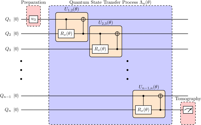
Figure 1: Circuit implementation of QST. Here, we prepare the initial states by implementing the $u_{3}$ operation in qubit $Q_{1}$. The states can be transferred to the $Q_{2}$ by applying the $U_{1,2}(\theta)$ operation decomposed with a CRX followed by a CNOT operation. We then iterate the $U_{l,l+1}(\theta)$ operation on the $n$-qubit chain. Finally, the states will be transferred to $Q_{n}$, which can then be obtained by the procedure of quantum state tomography.

III.1 State preparation

Because the IBM quantum experience does not allow one to access the post-measured states after Alice’s measurements, we prepare six eigenstates of Pauli matrices being Alice’s post-measurement states with indexes $x\in\{1,2,3\}$ and $a\in\{1,2\}$. Note that one can use the ancilla qubit, the CNOT operation, and the measurement operation on the ancilla qubit to replace the measurement operation on the system qubit Ku et al. (2020). Nevertheless, we consider the state preparation to avoid further errors from the CNOT operation. Note that the gate fidelity and the execution time of the CNOT operation are both at least $10$ times larger than the single qubit operation. Thus, to decrease the errors, the number of CNOT operations should be as less as possible. The initial state of the qubits on IBM quantum experience is always in $|0\rangle$. We can prepare $\tilde{\varrho}_{a|x}$ by applying the corresponding $u_{3}(\delta,\phi,\xi)$ operation at $Q_{1}$, mathematically as follows:

$$\tilde{\varrho}_{a|x}=u_{3}(\delta,\phi,\xi)|0\rangle\langle 0|u_{3}^{\dagger}(\delta,\phi,\xi),$$ (9)

with the matrix representation of the $u_{3}(\delta,\phi,\xi)$ operation being

$$u_{3}(\delta,\phi,\xi)=\begin{pmatrix}\cos{\frac{\delta}{2}}&-e^{i\xi}\sin{\frac{\delta}{2}}\\ e^{i\phi}\sin{\frac{\delta}{2}}&e^{i(\xi+\phi)}\cos{\frac{\delta}{2}}\end{pmatrix}.$$ (10)

Because we prepare the above states uniformly, $P_{\text{A}}(a|x)=0.5~{}~{}\forall~{}~{}a,x$, and the corresponding assemblage can be obtained by performing Pauli measurements on the maximally mixed state $\openone/2$. The above assemblage satisfies the NSIT condition in Eq. (5) and can maximize the spatiotemporal steering robustness Cavalcanti and Skrzypczyk (2016); Chen et al. (2020); Ku et al. (2018).

III.2 Quantum state transfer process

Figure 2: Schematic illustration of the perfect $n$-qubit QST process $\Lambda_{t}$, which consists of several iterations of quantum operations. For the $l$th iteration, the state is transferred from $Q_{l}$ to $Q_{l+1}$ by turning on the qubit-qubit interaction [depicted in Eq. (11) and Eq. (III.2)] for a period of time $\Delta t=\pi/(2J)$, where $J$ is $1/2$. Therefore, to transfer Alice’s prepared states from $Q_{1}$ to $Q_{n}$, the iteration has to be performed $n-1$ times.

We consider a QST process described by an $n$-qubit chain, as shown in Fig. 2, with each qubit labeled as $Q_{l}$, where $l=1,2,\dots,n$. In this process, Alice prepares the states in $Q_{1}$, and after the QST process, Bob will receive the transferred states in $Q_{n}$. We consider a QST procedure, which involves several iterations of quantum operations. For each iteration, we turn on the qubit-qubit interaction between $Q_{l}$ and $Q_{l+1}$, and then, turn it off when the QST from $Q_{l}$ to $Q_{l+1}$ is accomplished. Here, the “closed” interaction can be represented by the identity operator in the interaction Hamiltonian. The interaction Hamiltonian between $Q_{l}$ and $Q_{l+1}$ Li et al. (2018); Chen et al. (2017) is written as

$$H_{{l,l+1}}=\hbar J(\sigma_{l}^{+}\sigma_{l+1}^{-}+\sigma_{l}^{-}\sigma_{l+1}^{+}),$$ (11)

where $J$ is the coupling strength between $Q_{l}$ and $Q_{l+1}$. $\sigma_{l}^{+}(\sigma_{l}^{-})$ is the raising (lowering) operator acting on $Q_{l}$. Without loss of generality, $J$ can be set to $1/2$. The corresponding time evolution unitary operator can then be written as

$$\mathcal{V}_{l,l+1}(t) =\exp(-iH_{l,l+1}t/\hbar)$$

$$=\begin{pmatrix}1&0&0&0\\ 0&\cos{\frac{t}{2}}&-i\sin{\frac{t}{2}}&0\\ 0&-i\sin{\frac{t}{2}}&\cos{\frac{t}{2}}&0\\ 0&0&0&1\end{pmatrix}_{l,l+1},$$ (12)

where the matrix representation of the unitary operator is expanded in the computational basis for $Q_{l}$ and $Q_{l+1}$. Therefore, when the two qubit state is initialized in $\rho\otimes|0\rangle\langle 0|$, the reduced state $\rho^{\prime}$ for $Q_{l+1}$ after the evolved time $\Delta t=\pi$ reads as follows:

$$\rho^{\prime}=\text{Tr}_{l}[~{}\mathcal{V}_{l,l+1}(\Delta t)~{}(\rho\otimes|0\rangle\langle 0|)~{}\mathcal{V}_{l,l+1}^{\dagger}(\Delta t)~{}]=S^{\dagger}\rho S,$$ (13)

where $S=\text{diag}(1,i)$ is a unitary operator. Obviously, the state $\rho$ is perfectly transferred from $Q_{l}$ to $Q_{l+1}$ because the fidelity between the prepared and received states under the decoding unitary operation $S$ is unity. We note that the effective dynamics of the $\mathcal{V}_{l,l+1}(\Delta t)$ is identical to the $i$SWAP^† operation. If one of the subsystems is $|0\rangle$($|1\rangle$), the $i$SWAP^† operation can be viewed as a SWAP operation together with a $S^{\dagger}$($S$) operation. Also note that while considering the $XYZ$ interaction Hamiltonian in Ref. Kandel et al. (2019), the evolution operator is proportional to the SWAP operation.

Accordingly, to transfer Alice’s prepared states from $Q_{1}$ to $Q_{n}$, $n-1$ times of the aforementioned two-qubit operations are required. The total QST process can be described using the following unitary operation

$$\tilde{\mathcal{V}}_{1,n}=\prod_{l=n-1}^{1}\mathcal{V}_{l,l+1}~{},$$ (14)

Finally, the unitary $S^{n-1}$ is applied on $Q_{n}$, and Bob obtains the states that are the same as Alice’s prepared states. However, based on Eq. (8), the decoding unitary operation $S^{n-1}$ is unnecessary when considering the STS scenario. Usually, for digital quantum processors, e.g. the IBM quantum experience and QuTech quantum inspire considered in this work, the $S^{n-1}$ operation comprises a sequence $S$-gate.

The circuit implementation of the evolution operator $\mathcal{V}_{l,l+1}(\theta)$ in Eq. (III.2) is shown in Fig. 3a. Here, we replace $t$ with $\theta$. To implement the controlled rotation $X$ (CRX) in IBM quantum experience, one has to decompose it with two CNOT operations and three $u_{3}$ operations. Thus, there are a total of four CNOT operations in the evolution operator $\mathcal{V}_{l,l+1}(\theta)$. As mentioned above, we would like to decrease the number of the CNOT operations to decrease the inevitable errors. Thus, we consider an alternative unitary operator $U_{l,l+1}(\theta)$, which reduces one CNOT operation, as

$$U_{l,l+1}(\theta)=\begin{pmatrix}1&0&0&0\\ 0&0&-i\sin{\frac{\theta}{2}}&\cos{\frac{\theta}{2}}\\ 0&0&\cos{\frac{\theta}{2}}&-i\sin{\frac{\theta}{2}}\\ 0&1&0&0\end{pmatrix}_{l,l+1},$$ (15)

where the circuit implementation of $U_{l,l+1}$ is shown in Fig. 3b. If the initial state in $Q_{l+1}$ is always $|0\rangle\langle 0|$, we can replace $\mathcal{V}_{l,l+1}$ with $U_{l,l+1}$; thus, Eq. (13) still holds, where

$$\rho^{\prime} =\text{Tr}_{l}[\mathcal{V}_{l,l+1}(\theta)(\rho\otimes|0\rangle\langle 0|)\mathcal{V}_{l,l+1}^{\dagger}(\theta)]$$

$$=\text{Tr}_{l}[U_{l,l+1}(\theta)(\rho\otimes|0\rangle\langle 0|)U_{l,l+1}^{\dagger}(\theta)].$$ (16)

For this implementation, the QST process is perfect only when $\theta=\pi$, that is, $\rho$ and $\rho^{\prime}$ are related by unitary operation $S$. We refer to the cases where $\theta\neq\pi$ as imperfect QST processes because the transferred states cannot be transformed to the prepared states through an decoding unitary transformation.

(a) $\mathcal{V}_{l,l+1}(\theta)$

(b) $U_{l,l+1}(\theta)$

Figure 3: Circuit decomposition of $\mathcal{V}_{l,l+1}(\theta)$ and $U_{l,l+1}(\theta)$. $R_{x}(\theta)$ is the rotation $X$ operation with rotating angle $\theta$.

III.3 Ideal theoretical results

Figure 4 shows theoretical predictions of $\mathcal{STSR}$ with respect to the parameter $\theta$ for different qubit numbers $n\in\{2,3,4,5\}$. We can observe that for fixed $n$, the value of $\mathcal{STSR}$ for the perfect QST case ($\theta=\pi$) is always larger than those for the imperfect QST cases ($\theta\neq\pi$). This is because for a fixed $n$, the assemblages for the $\theta=\pi$ case and those for the $\theta\neq\pi$ cases are, in general, related by a unitary transformation and a completely positive and trace-preserving map (CPTP), respectively. It has been proved that $\mathcal{STSR}$ monotonically decreases whenever the underlying assemblage is sent into a CPTP map Gallego and Aolita (2015).

Moreover, for fixed $\theta$, the value of the $\mathcal{STSR}$ monotonically decreases with increasing qubit number $n$. As shown in Figs. 1 and 2, increasing $n$ means increasing the number of the iterations required in the QST process. As described in Eq. (III.2), for each iteration, the input state $\rho$ and the output state $\rho^{\prime}$ can also be generally related by a CPTP map. Therefore, when increasing the number $n$, the prepared assemblage will be iteratively sent into the CPTP maps, which results in a decrease of the $\mathcal{STSR}$ Gallego and Aolita (2015).

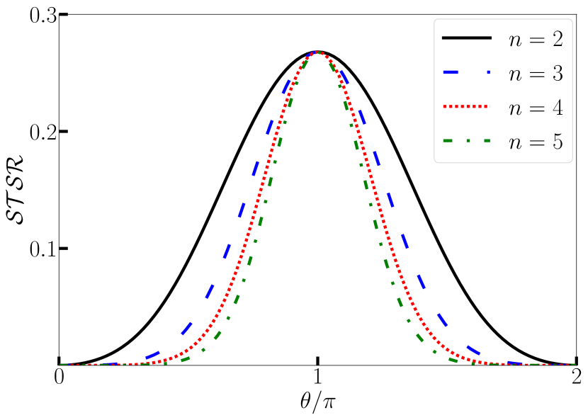
Figure 4: Value of $\mathcal{STSR}$ with respect to different angle $\theta$ for different qubit number $n$. Here, the initial assemblage for $Q_{1}$ is $\{\varrho_{a|x}=P_{\text{A}}(a|x)\tilde{\varrho}_{a|x}\}_{a,x}$ where $P_{\text{A}}(a|x)=1/2$ for all $a,x$ and $\tilde{\varrho}_{a|x}$ are the eigenstates of Pauli operators.

III.4 Noise simulation

Because the quantum devices nowadays suffer from noise due to the interactions with environments Johansson et al. (2012, 2013), we model the noise effect by introducing extra qubit decoherence (dephasing and relaxation) described by the following Lindblad master equation (similar discussions can be found in the Ref. Ku et al. (2020)):

$$\dot{\rho}(t) =\sum_{l}^{n}\hbar\frac{\gamma^{l}_{T_{1}}}{2}\left[2\sigma_{-}^{l}\rho(t)\sigma_{+}^{l}-\sigma_{+}^{l}\sigma_{-}^{l}\rho(t)-\rho(t)\sigma_{+}^{l}\sigma_{-}^{l}\right]$$ (17)

$$+\sum_{l}^{n}\hbar\frac{\gamma^{l}_{T_{2}}}{2}\left[2\sigma_{z}^{l}\rho(t)\sigma_{z}^{l}-{\sigma_{z}^{l}}^{2}\rho(t)-\rho(t){\sigma_{z}^{l}}^{2}\right],$$

where $\rho$ denotes the density operator for the total n-qubit system, and the coefficients $\gamma^{l}_{T_{1}}=1/T_{1}^{l}$ and $\gamma_{T_{2}}^{l}=(1/T_{2}^{l}-1/2T_{2}^{l})/2$ are the qubit relaxation and decoherence rates for $Q_{l}$, respectively. Here, $T_{1}^{l}$ and $T_{2}^{l}$ represent the relaxation and dephasing time for $Q_{l}$, respectively. The relaxation and the coherence time for each qubit and the operation-execution time are all public in IBM quantum experience IBM . We use these public information together with the master equation to model the decoherence effect for real devices, such that the final reduced state $\rho_{n}$ of $Q_{n}$ can be obtained when tracing out other qubits.

We further consider the measurement (readout) errors, which is not described in the aforementioned master equation. To insert such errors, we briefly recall how to obtain measurement errors in IBM quantum experience. In the measurement-error calibration, we always measure the system in computational basis while initializing the qubit with two basis states, $|0\rangle$ and $|1\rangle$. For the ideal situation, the measurement outcome is $0$ ($1$) with certainty when the qubit is initialized in $|0\rangle$ ($|1\rangle$). Therefore, measurement errors $\Gamma$ can be determined by the average probability of preparation in $|0\rangle(|1\rangle)$ with the opposite outcome $1$ ($0$). We model such errors by sending the quantum state into the bit-flip channel before measurement; i.e.,

$$\rho_{n}\rightarrow(1-\Gamma)\rho_{n}+\Gamma X\rho_{n}X^{\dagger}.$$ (18)

The above channel changes the population of the quantum state $\rho_{n}$ with probability $\Gamma$. Notably, once the state is $|0\rangle$ or $|1\rangle$, the population obtained by the above is the same as the one in the measurement-error calibration. Finally, we emphasize that since both Eq. (17) and Eq. (18) can be described by CPTP maps, $\mathcal{STSR}$ can only decrease Gallego and Aolita (2015) after introducing our noisy model.

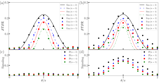
Figure 5: The experimental values of the $\mathcal{STSR}$ under the QST. The evolution operators transfer the state from $Q_{1}$ to $Q_{n}$. The experimental results of (a) and (c) are implemented in Mar 2020 after maintenance, whereas those for (b) and (d) were complete in Jan 2020 before the maintenance. In (a) and (b), we show the spatiotemporal steerability as a quantification of the QST process. When $\theta=\pi$, the ideal evolution circuit, corresponding to the perfect QST process, provides the maximal spatiotemporal steerability. Although the experimental $\mathcal{STSR}$ cannot reach the theoretical prediction, the trend of the experimental results functions similarly with the ideal case. Moreover, one can observe that the $\mathcal{STSR}$ well fitted the noisy model for (a) and (b). One can see that the signaling effect in (d) actually dominates $\mathcal{STSR}$ in (b) by Eq. (6).

IV Experimental Results

We prepare the eigenstates of Pauli matrices in $Q_{1}$ using the corresponding single-quantum operation $u_{3}$, which rotates the $|0\rangle$ to the prepared states (see Sec. III.1). The global evolution $\Lambda_{n}(\theta)$ is then applied as shown in Fig. 1 with different qubit numbers $n\in\{2,3,4,5\}$. After sending the system into the channel $\Lambda_{n}(\theta)$, we can reconstruct the reduced density matrices on $Q_{n}$ by standard state tomography. Here, the measurement results are obtained through $8000$ shots for each procedure in the state tomography.

In Fig. 5, we present experimental data with $\theta\in\{\frac{m\pi}{7}|m=0,1,...,14\}$ obtained from different dates on March 2020 and January 2020 for the same device named IBMQ boeblingen. The experiment shown in Fig. 5 (a) and (c) was completed right after maintenance, whereas the results in Fig. 5 (b) and (d) were obtained before the maintenance. We also provide the noise simulation mentioned in Sec. III.4 and the violation of the NSIT described in Eq. (6). One can find that the value of the $\mathcal{STSR}$ at $\theta=\pi$, where the perfect QST occurs for the ideal case, decreases as the qubit number $n$ increases. The reduction agrees with the noise simulations, suggesting that the QST nonclassicality is suppressed because of accumulation of noise. Additionally, It seems that the overall $\mathcal{STSR}$ or the QST nonclassicality for the result before the maintenance are larger than that after maintenance. However, by observing Fig. 5(c) and Fig. 5(d), we can clearly find that the $\mathcal{STSR}$ before the maintenance, as shown in Fig. 5(b), is actually dominated by the signaling effect, which cannot be regarded as a genuine quantumness. Therefore, benchmarking nonclassicality of a quantum device requires both $\mathcal{STSR}$ and the condition of NSIT.

Furthermore, there exists intrinsic non-Markovianity in the quantum processors Morris et al. (2019); Harper and Flammia (2019). The non-Markovianity is a possible source of the violation of NSIT shown in the presented experimental results because the existence of the non-Markovian effect implies that the operations shown in Fig. 1 could not be divisible. In other words, the global evolution $\Lambda_{n}(\theta)$ could depend on the state preparation operation $u_{3}$ and could result in the violation of Eq. (5).

Finally, the experimental results of the perfect QST from the other quantum devices based on spin qubits (QuTech spin-2) in silicon Vandersypen et al. (2017); Watson et al. (2018) and the superconducting transmon qubits (QuTech starmon-5) are also presented in Table. 1. Because QuTech devices do not support the generalized $u_{3}$ and CNOT operation (one has to decompose the arbitrary quantum operations by a serious single quantum operations and the CZ operations), we only consider the perfect QST case which can be decomposed by $H,S,Z$, and CNOT operations. The qubit relation time ($T_{1}$) and the coherence time ($T_{2}$) given by IBM quantum experience IBM is about six to eight times longer than those given by QuTech quantum inspire QuTech (2018). Generally speaking, IBM quantum experience outperforms QuTech quantum inspire when both the $\mathcal{STSR}$ and singalling effect are considered. This could be because of the unwanted operation decompositions on the CRX and the CNOT operation such that the noise effect and circuit depth increase. The signaling effect in QuTech spin-2 dominates the result, just like IBMQ’s results before maintenance. We also present $\mathcal{STSR}$ under the perfect QST process on other IBM quantum devices (in Appendix D).

Table 1: The values of the $\mathcal{STSR}$ under the perfect QST process with different quantum devices. Here, we consider the IBMQ boeblingen, QuTech starmon-5, and spin-2 systems. The transference route initially begins with the preparation in $Q_{0}$, passing through the intermediary qubits, and performs state tomography on the final qubit. The experimental results of the signaling effect are also presented.

Devices	Transference routes	$~{}n~{}$	$~{}\mathcal{STSR}~{}$	Signaling
IBMQ boeblingen (Mar, 2020)	$0\to 1\to 2\to 3\to 4$	2	0.216	0.015
		3	0.202	0.018
		4	0.173	0.019
		5	0.129	0.026
QuTech starmon-5 (May, 2020)	$0\to 2\to 4$	2	0.170	0.051
		3	0.054	0.035
QuTech spin-2 (May, 2020)	$0\to 1$	2	0.103	0.100

V Discussion

In this work, we first defined the classical strategy of state transfer as the received state can be constructed by an ensemble of ontic states together with a stochastic map. Such a strategy can be described by the local-hidden-state model which is widely used in the context of the steering scenarios. We then proposed a method based on STS to quantify the nonclassicality of the QST process. We have shown that the spatiotemporal steerability is invariant under the process of the perfect QST, whereas the reduction during the process of the QST is imperfect. Moreover, we have provided a quantity to estimate signaling effect and proved that such a quantity is a lower bound of $\mathcal{STSR}$.

Not only did we realize a proof-of-principle experiment but also performed a benchmark experiment of the QST process on IBM quantum experience and QuTech quantum inspire. Our experimental results show that the degrees of QST nonclassicality decrease as the circuit depth increases. In addition, the decrease agrees with the noise model, which describes the accumulation of noise (qubit relaxation, gate error, and readout error) during the QST process. The experimental results from the IBMQ boeblingen before the maintenance shows that the spatiotemporal steerability is actually dominated by the signaling effect. Such signaling effect could be caused by the intrinsic non-Markovianity for the quantum devices.

In Ref. Bayat and Bose (2010), it has been shown that the average fidelity of the QST process is identical to estimate the degree of entanglement distribution. More specifically, by keeping one part of the maximally entanglement pair in the sender and sending the other part to receiver through QST process, we can compute the singlet fraction of the output state  Horodecki et al. (1999). The above approach has been used to quantify the QST process Horodecki et al. (1999). In general, this output state is the Choi state, which is the one-to-one mapping between the quantum state and quantum channel. We recall that the degree of the entanglement can be estimated by spatial steerability Uola et al. (2020); Zhao et al. (2020); Chen et al. (2020); Piani and Watrous (2015). Furthermore, violating the steering inequality is related to the singlet fraction Hsieh et al. (2016). Due to the hierarchy relation in Ref. Ku et al. (2018), STS can access partial information of the Choi state. Therefore, it is naturally to ask whether spatiotemporal steerability can estimate the amount of entanglement distribution.

Throughout this work, although we only consider the single-qubit QST, we briefly discuss the $d$-level Bayat (2014); Liu et al. (2017) and multi-partite QST Lorenzo et al. (2013). Since, in Eq. (1), the dimension of the prepared and received states can be arbitrary, our approach can be easily extended to $d$-level QST. It would be more interesting to consider multi-partite QST. In such a scenario, depending on the structure of the assemblage, one could introduce more constraints on the ontic states in LHS model Cavalcanti et al. (2015). For instance, consider the case where the assemblage contains two sets of two-qubit entangled states, there are at least two different ways to define the ontic states in LHS model: One could either allow the ontic states to be arbitrary or separable two-qubit states. Therefore, the nonclassicality of multi-partite QST could be very versatile (e.g., the ontic states could be $m$-separable in the notion of genuine multi-partite entanglement Cavalcanti et al. (2015); Zhou et al. (2019); Lu et al. (2018); Gühne and Tóth (2009)).

This work also raises some open questions. Can we characterize the non-Markovian effect? Can we implement the QST process with less CNOT operations? In our work, we have to use three CNOT operations to implement QST, while the number of the CNOT operations is the same as the operation decomposition of the SWAP operation.

Appendix A Semidefinite programming for spatiotemporal steering robustness

Here, we briefly describe the semidefinite program (SDP) of the spatiotemporal steering robustness $\mathcal{STSR}$ in Eq. (4) which is first introduced in Chen et al. (2017). We also note that the SDP of the $\mathcal{STSR}$ is identical to that in the spatial and temporal steering scenarios Piani and Watrous (2015); Ku et al. (2016); Cavalcanti and Skrzypczyk (2016).

Let us consider $m$-measurement settings $x\in\{1,2,...,m\}$ where each has $q$ outcomes $a\in\{1,2,...,q\}$. Since inputs and outcomes are finite, the number of the variable $\lambda$ in Eq. (3) is $q^{m}$. Each $\lambda$ can be considered as a string of ordered outcomes according to the measurements: $(a_{x=1},a_{x=2},...,a_{x=m})$. We can define the deterministic strategy function $D_{\lambda}(a|x)=\delta_{a,\lambda(x)}$, where $\delta$ is the Kronecker delta function and $\lambda(x)$ denotes the value of the string at position $x$ Uola et al. (2020); Cavalcanti and Skrzypczyk (2016). Therefore, given an assemblage $\{\varrho_{a|x}\}$, the primal SDP of $\mathcal{STSR}$ can be formulated as follows (see the derivation in Refs. Cavalcanti and Skrzypczyk (2016); Uola et al. (2020)):

$${\displaystyle\min_{\{\sigma_{\lambda}\}}} \text{Tr}\sum_{\lambda}\sigma_{\lambda}-1,$$

s.t. $$\sum_{\lambda}D_{\lambda}(a|x)\sigma_{\lambda}-\varrho_{a|x}\geq 0~{}~{}\forall~{}a,x~{},$$

$$\sigma_{\lambda}\geq 0~{}~{}\forall~{}\lambda~{}.$$ (19)

The dual formulation of Eq. (A) is given by Cavalcanti and Skrzypczyk (2016); Uola et al. (2020)

$${\displaystyle\max_{\{F_{a|x}\}}} \text{Tr}\sum_{a,x}F_{a|x}\varrho_{a|x}-1,$$

s.t. $$\openone-\sum_{a,x}D_{\lambda}(a|x)F_{a|x}\geq 0~{}~{}\forall~{}\lambda~{},$$

$$F_{a|x}\geq 0~{}~{}\forall~{}a,x.$$ (20)

Here, $F_{a|x}$ is the steering witness that distinguishes the steerable assemblage from the unsteerable ones. We note that the strong duality of $\mathcal{STSR}$ has been shown in Refs. Clemente and Kofler (2015); Cavalcanti and Skrzypczyk (2016), meaning that the results of the primal and dual formulations are equivalent.

Appendix B Proof of Eq. (8) in the main text

In this section, we show that given an assemblage $\{\varrho_{a|x}\}$, the $\mathcal{STSR}$ is invariant under unitary transformation using the strong duality mentioned in Appendix A. More specifically, we show $\mathcal{STSR}(\{\varrho_{a|x}^{\prime}\})=\mathcal{STSR}(\{\varrho_{a|x}\})$, where $\varrho_{a|x}^{\prime}=U\varrho_{a|x}U^{\dagger}$ with $U$ being an arbitrary unitary operator.

Because the dual formulation of SDP in Eq. (A) of $\mathcal{STSR}$ is strongly feasible, given an assemblage $\{\varrho_{a|x}\}$, one can always find the optimal spatiotemporal steering witness $\{F_{a|x}^{*}\}$ satisfying both constraints in Eq. (A):

$$\mathcal{STSR}(\{\varrho_{a|x}\})=\text{Tr}\sum_{a,x}F_{a|x}^{*}\varrho_{a|x}-1.$$

With the above, we now apply a unitary transformation $U$ on the given assemblage $\{\varrho_{a|x}\}$. The dual formulation of $\mathcal{STSR}(\{\varrho_{a|x}^{\prime}\})$ can be expressed as follows:

$$\mathcal{STSR}(\{\varrho_{a|x}^{\prime}\}) ={\displaystyle\max_{\{F_{a,x}^{\prime}\}}}~{}\text{Tr}\sum_{a,x}F_{a|x}^{\prime}\varrho_{a|x}^{\prime}-1$$

$$\geq\text{Tr}\sum_{a,x}(UF_{a|x}^{*}U^{\dagger})(U\varrho_{a|x}U^{\dagger})-1$$

$$=\text{Tr}\sum_{a,x}UF_{a|x}^{*}\varrho_{a|x}U^{\dagger}-1$$

$$=\text{Tr}\sum_{a,x}F_{a|x}^{*}\varrho_{a|x}-1$$

$$=\mathcal{STSR}(\{\varrho_{a|x}\})~{}.$$

The inequality holds because $\{UF_{a|x}^{*}U^{\dagger}\}$ is not the optimal solution of SDP. Nevertheless, it is indeed a valid solution because it satisfies both constraints in Eq. (A):

$$\openone-\sum_{a,x}D_{\lambda}(a|x)F_{a|x}^{\prime} =\openone-\sum_{a,x}D_{\lambda}(a|x)UF_{a|x}^{*}U^{\dagger}$$

$$=U\left(\openone-\sum_{a,x}D_{\lambda}(a|x)F_{a|x}^{*}\right)U^{\dagger}$$

$$\geq 0~{}~{}\forall~{}\lambda~{},$$

$$F_{a|x}^{\prime}=UF_{a|x}^{*}U^{\dagger}\geq 0~{}~{}\forall~{}a,x.$$

Therefore, we arrive at the bound relation; i.e.,

$$\mathcal{STSR}(\{\varrho_{a|x}^{\prime}\})\geq\mathcal{STSR}(\{\varrho_{a|x}\}).$$ (21)

A similar argument can also be applied to the primal SDP in Eq. (A) of $\mathcal{STSR}$. Given an assemblage, one can always find the optimal $\{\sigma_{\lambda}^{*}\}$ that satisfies both constraints in Eq. (A):

$$\mathcal{STSR}(\{\varrho_{a|x}\})=\text{Tr}\sum_{\lambda}\sigma_{\lambda}^{*}-1.$$

By applying a unitary transformation $U$ on the given assemblage $\{\varrho_{a|x}\}$, the primal SDP of $\mathcal{STSR}(\{\varrho_{a|x}^{\prime}\})$ can then be expressed as follows:

$$\mathcal{STSR}(\{\varrho_{a|x}^{\prime}\}) ={\displaystyle\min_{\{\sigma_{\lambda}^{\prime}\}}}~{}\text{Tr}\sum_{\lambda}\sigma_{\lambda}^{\prime}-1$$

$$\leq\text{Tr}\sum_{\lambda}U\sigma_{\lambda}^{*}U^{\dagger}-1$$

$$=\text{Tr}\sum_{\lambda}\sigma_{\lambda}^{*}-1$$

$$=\mathcal{STSR}(\{\varrho_{a|x}\})~{}.$$

The inequality holds because $\{U\sigma_{\lambda}^{*}U^{\dagger}\}$ is not the optimal solution of the SDP. Nevertheless, it is indeed a valid solution because it satisfies both constraints in Eq. (A):

$$\sum_{\lambda}D_{\lambda}(a|x)\sigma_{\lambda}^{\prime}-\varrho_{a|x}^{\prime} =\sum_{\lambda}D_{\lambda}(a|x)U\sigma_{\lambda}^{*}U^{\dagger}-U\varrho_{a|x}U^{\dagger}$$

$$=U\left(\sum_{\lambda}D_{\lambda}(a|x)\sigma_{\lambda}^{*}-\varrho_{a|x}\right)U^{\dagger}$$

$$\geq 0~{}~{}\forall~{}a,x~{},$$

$$\sigma_{\lambda}^{\prime}=U\sigma_{\lambda}^{*}U^{\dagger}\geq 0~{}~{}\forall~{}\lambda~{}.$$

Therefore, we arrive at another bound relation which is given as

$$\mathcal{STSR}(\{\varrho_{a|x}^{\prime}\})\leq\mathcal{STSR}(\{\varrho_{a|x}\}).$$ (22)

There are some similar properties of Eq. (22) that have been discussed in Ref. Gallego and Aolita (2015).

By combining Eq. (21) and Eq. (22), we find that $\mathcal{STSR}$ of the assemblage is invariant under unitary transformation:

$$\mathcal{STSR}(\{U\varrho_{a|x}U^{\dagger}\})=\mathcal{STSR}(\{\varrho_{a|x}\}),$$ (23)

thus, we have completed the proof that perfect state transfer implies invariance of $\mathcal{STSR}$. $\blacksquare$

Appendix C Proof of Eq. (7) in the main text

We now briefly summarize how to obtain the bound relation in Eq. (7) by additionally introducing two optimization problems ($\mathcal{R}_{1}$ and $\mathcal{R}_{2}$). We then show the bound relations of each optimization problems, namely (1) $\mathcal{STSR}\geq\mathcal{R}_{1}$, (2) $\mathcal{R}_{1}\geq\mathcal{R}_{2}$, (3) $\mathcal{R}_{2}\geq\mathcal{D}$. Due to the transitivity, we can complete the proof.

Once the NSIT condition is not satisfied, the marginal of the assemblage can be defined as $\varrho_{x}=\sum_{a}\varrho_{a|x}$. Motivated by the definition of $\mathcal{STSR}$ in Eq. (4), it is convenient to introduce the first optimization problem, namely

$$\mathcal{R}_{1}(\{\varrho_{a|x}\}) =\displaystyle\min_{r_{1},\{\tau_{x}\},\sigma}~{}~{}r_{1},$$

$$\text{s.t.}~{}~{}~{}\frac{\varrho_{x}+r_{1}\tau_{x}}{1+r_{1}}=\sigma~{}~{}~{}\forall~{}~{}~{}x,$$ (24)

where $\sigma$ and $\tau_{x}$ are arbitrary quantum states. It is easy to see that the above optimization problem is merely the robustness without the NSIT condition, and the corresponding SDP can be easily derived. We note that whether the above robustness has the corresponding resource theory is still vague Chitambar and Gour (2019). It is easy to discover that the optimal solution for Eq. (4) (denoted as $r^{*}$, $\{\tau_{a|x}^{*}\}$, and $\{(\varrho_{a|x}^{\text{LHS}})^{*}\}$) is a valid solution for Eq. (C) because it satisfies all the constraints in Eq. (C) by introducing $\tau_{x}=\sum_{a}\tau_{a|x}^{*}$ and $\sigma=\sum_{a}(\varrho_{a|x}^{\text{LHS}})^{*}$. Nevertheless, it may not be the optimal solution for Eq. (C). Therefore, we have the first bound relation

$$\mathcal{STSR}(\{\varrho_{a|x}\})\geq\mathcal{R}_{1}(\{\varrho_{a|x}\}).$$ (25)

Since the right-hand side of the constraint in Eq. (C) is independent of $x$, we can reformulate Eq. (C) as

$$\mathcal{R}_{1} (\{\varrho_{a|x}\})=\displaystyle\min_{r_{1},\{\tau_{x}\}}~{}~{}r_{1},$$

$$\text{s.t.}~{}~{}~{}r_{1}(\tau_{x}-\tau_{x^{\prime}})=\varrho_{x^{\prime}}-\varrho_{x}~{}~{}~{}\forall~{}x\neq x^{\prime}.$$ (26)

With the above results, we can further introduce another optimization problem, namely

$$\mathcal{R}_{2} (\{\varrho_{a|x}\})=\displaystyle\min_{r_{2},\{\tau_{x}\}}~{}~{}r_{2},$$

$$\text{s.t.}~{}~{}~{}r_{2}||\tau_{x}-\tau_{x^{\prime}}||_{1}=||\varrho_{x}-\varrho_{x^{\prime}}||_{1}~{}~{}~{}\forall~{}x\neq x^{\prime}.$$ (27)

The Eq. (C) and Eq. (C) satisfy the following bound relation

$$\mathcal{R}_{1}(\{\varrho_{a|x}\})\geq\mathcal{R}_{2}(\{\varrho_{a|x}\}).$$ (28)

The inequality holds because the optimal solution in Eq. (C) is also a valid but not optimal solution for Eq. (C).

Now, consider $r^{*}_{2}$ and $\{\tau_{x}^{*}\}$ to be the optimal solution for Eq. (C), it must satisfy the constraint, namely

$$r_{2}^{*}~{}||\tau^{*}_{x}-\tau^{*}_{x^{\prime}}||_{1}=||\varrho_{x}-\varrho_{x^{\prime}}||_{1}~{}~{}~{}\forall~{}x\neq x^{\prime}.$$

Because the maximum value of the trace norm between two arbitrary quantum states is $2$, i.e., $||\tau_{x}^{*}-\tau^{*}_{x^{\prime}}||_{1}\leq 2$, we have

$$r_{2}^{*}\geq\frac{1}{2}||\varrho_{x}-\varrho_{x^{\prime}}||_{1}~{}~{}~{}\forall~{}x\neq x^{\prime},$$

or alternatively,

$$r^{*}_{2}\geq\max_{x}~{}\frac{1}{2}||\varrho_{x}-\varrho_{x^{\prime}}||_{1}~{}~{}\forall~{}~{}x\neq x^{\prime}.$$

Therefore, we arrive at the last bound relation

$$\mathcal{R}_{2}(\{\varrho_{a|x}\}) =r^{*}_{2}$$

$$\geq\max_{x}~{}\frac{1}{2}\left|\left|\sum_{a}\varrho_{a|x}-\sum_{a}\varrho_{a|x^{\prime}}\right|\right|_{1}~{}~{}\forall~{}~{}x\neq x^{\prime}$$

$$=\mathcal{D}(\{\varrho_{a|x}\}).$$ (29)

Finally, due to the transitivity, we complete the proof, namely

$$\mathcal{STSR}\geq\mathcal{R}_{1}\geq\mathcal{R}_{2}\geq\mathcal{D}.~{}\blacksquare$$ (30)

Appendix D The experimental results from different IBMQ devices

In Table. 2, we show $\mathcal{STSR}$ under the process of the perfect QST with different IBMQ devices: 20-qubits almaden, 20-qubits boeblingen, 28-qubits cambridge, 5-qubits london, and 27-qubits paris. The circuit implementations for all are the same as the one introduced in the main text (see Sec. III.1 and Sec. III.2). One can see that the different chips shows different performances of the QST. We thus can benchmark each chips under the QST tasks.

Table 2: Experimental results of the perfect QST ($\theta=\pi$) from different IBMQ devices.

Devices	Transference routes	$~{}n~{}$	$~{}\mathcal{STSR}~{}$	Signaling
almaden (Mar, 2020)	$0\to 1\to 2\to 3\to 4$	2	0.169	0.026
		3	0.130	0.021
		4	0.086	0.019
		5	0.040	0.021
almaden (Mar, 2020)	$5\to 6\to 7\to 8\to 9$	2	0.133	0.025
		3	0.040	0.025
		4	0.016	0.015
		5	0.018	0.018
boeblingen (Mar, 2020)	$0\to 1\to 2\to 3\to 4$	2	0.216	0.015
		3	0.202	0.018
		4	0.173	0.019
		5	0.129	0.026
boeblingen (Jan, 2020)	$0\to 1\to 2\to 3\to 4$	2	0.231	0.184
		3	0.198	0.153
		4	0.170	0.140
		5	0.140	0.138
boeblingen (Mar, 2020)	$5\to 6\to 7\to 8\to 9$	2	0.059	0.024
		3	0.133	0.025
		4	0.116	0.030
		5	0.033	0.030
boeblingen (Mar, 2020)	$15\to 16\to 17\to 18\to 19$	2	0.025	0.021
		3	0.032	0.027
		4	0.010	0.010
		5	0.005	0.005
cambridge (Jul, 2020)	$0\to 1\to 2\to 3\to 4$	2	0.017	0.017
		3	0.006	0.006
		4	0.009	0.008
		5	0.011	0.011
london (Oct, 2019)	$0\to 1\to 3\to 4$	2	0.203	0.022
		3	0.190	0.027
		4	0.154	0.029
paris (Jul, 2020)	$0\to 1\to 2\to 3\to 5$	2	0.208	0.074
		3	0.197	0.087
		4	0.148	0.039
		5	0.085	0.061

References

- Kay (2010) A. Kay, Perfect, efficient, state transfer and its application as a constructive tool, Int. J. Quantum Inf. 08, 641–676 (2010).
- Christandl et al. (2004) M. Christandl, N. Datta, A. Ekert, and A. J. Landahl, Perfect state transfer in quantum spin networks, Phys. Rev. Lett. 92, 187902 (2004).
- Lvovsky et al. (2009) A. I. Lvovsky, B. C. Sanders, and W. Tittel, Optical quantum memory, Nat. Photonics 3, 706 (2009).
- Yuan et al. (2019) X. Yuan, Y. Liu, Q. Zhao, B. Regula, J. Thompson, and M. Gu, Robustness of quantum memories: An operational resource-theoretic approach, arXiv:1907.02521 (2019).
- Rosset et al. (2018) D. Rosset, F. Buscemi, and Y.-C. Liang, Resource theory of quantum memories and their faithful verification with minimal assumptions, Phys. Rev. X 8, 021033 (2018).
- Cirac et al. (1997) J. I. Cirac, P. Zoller, H. J. Kimble, and H. Mabuchi, Quantum state transfer and entanglement distribution among distant nodes in a quantum network, Phys. Rev. Lett. 78, 3221 (1997).
- Chiribella et al. (2009) G. Chiribella, G. M. D’Ariano, and P. Perinotti, Theoretical framework for quantum networks, Phys. Rev. A 80, 022339 (2009).
- Hahn et al. (2019) F. Hahn, A. Pappa, and J. Eisert, Quantum network routing and local complementation, npj Quantum Inf. 5, 76 (2019).
- Khatri et al. (2021) S. Khatri, A. J. Brady, R. A. Desporte, M. P. Bart, and J. P. Dowling, Spooky action at a global distance: analysis of space-based entanglement distribution for the quantum internet, npj Quantum Inf. 7, 4 (2021).
- Lu et al. (2019) H. Lu, Z.-D. Li, X.-F. Yin, R. Zhang, X.-X. Fang, L. Li, N.-L. Liu, F. Xu, Y.-A. Chen, and J.-W. Pan, Experimental quantum network coding, npj Quantum Inf. 5, 89 (2019).
- Bennett et al. (1993) C. H. Bennett, G. Brassard, C. Crépeau, R. Jozsa, A. Peres, and W. K. Wootters, Teleporting an unknown quantum state via dual classical and Einstein-Podolsky-Rosen channels, Phys. Rev. Lett. 70, 1895 (1993).
- Schmidt-Kaler et al. (2003) F. Schmidt-Kaler, H. Häffner, M. Riebe, S. Gulde, G. P. T. Lancaster, T. Deuschle, C. Becher, C. F. Roos, J. Eschner, and R. Blatt, Realization of the cirac–zoller controlled-NOT quantum gate, Nature 422, 408 (2003).
- Yao et al. (2011) N. Y. Yao, L. Jiang, A. V. Gorshkov, Z.-X. Gong, A. Zhai, L.-M. Duan, and M. D. Lukin, Robust quantum state transfer in random unpolarized spin chains, Phys. Rev. Lett. 106, 040505 (2011).
- Kandel et al. (2019) Y. P. Kandel, H. Qiao, S. Fallahi, G. C. Gardner, M. J. Manfra, and J. M. Nichol, Coherent spin-state transfer via Heisenberg exchange, Nature 573, 553 (2019).
- Lorenzo et al. (2013) S. Lorenzo, T. J. G. Apollaro, A. Sindona, and F. Plastina, Quantum-state transfer via resonant tunneling through local-field-induced barriers, Phys. Rev. A 87, 042313 (2013).
- Bayat and Bose (2010) A. Bayat and S. Bose, Information-transferring ability of the different phases of a finite xxz spin chain, Phys. Rev. A 81, 012304 (2010).
- Bayat (2014) A. Bayat, Arbitrary perfect state transfer in -level spin chains, Phys. Rev. A 89, 062302 (2014).
- Rueda et al. (2019) A. Rueda, W. Hease, S. Barzanjeh, and J. M. Fink, Electro-optic entanglement source for microwave to telecom quantum state transfer, npj Quantum Inf. 5, 108 (2019).
- Liu et al. (2017) T. Liu, Q.-P. Su, J.-H. Yang, Y. Zhang, S.-J. Xiong, J.-M. Liu, and C.-P. Yang, Transferring arbitrary d-dimensional quantum states of a superconducting transmon qudit in circuit QED, Sci. Rep. 7, 7039 (2017).
- Lau and Clerk (2019) H.-K. Lau and A. A. Clerk, High-fidelity bosonic quantum state transfer using imperfect transducers and interference, npj Quantum Inf. 5, 31 (2019).
- Schrödinger (1935) E. Schrödinger, Discussion of probability relations between separated systems, Proc. Cambridge Phil. Soc. 31, 555 (1935).
- Einstein et al. (1935) A. Einstein, B. Podolsky, and N. Rosen, Can quantum-mechanical description of physical reality be considered complete?, Phys. Rev. 47, 777 (1935).
- Wiseman et al. (2007) H. M. Wiseman, S. J. Jones, and A. C. Doherty, Steering, entanglement, nonlocality, and the Einstein-Podolsky-Rosen paradox, Phys. Rev. Lett. 98, 140402 (2007).
- Uola et al. (2020) R. Uola, A. C. S. Costa, H. C. Nguyen, and O. Gühne, Quantum steering, Rev. Mod. Phys. 92, 015001 (2020).
- Cavalcanti et al. (2009) E. G. Cavalcanti, S. J. Jones, H. M. Wiseman, and M. D. Reid, Experimental criteria for steering and the Einstein-Podolsky-Rosen paradox, Phys. Rev. A 80, 032112 (2009).
- Cavalcanti and Skrzypczyk (2016) D. Cavalcanti and P. Skrzypczyk, Quantum steering: a review with focus on semidefinite programming, Rep. Prog. Phys. 80, 024001 (2016).
- Piani and Watrous (2015) M. Piani and J. Watrous, Necessary and sufficient quantum information characterization of einstein-podolsky-rosen steering, Phys. Rev. Lett. 114, 060404 (2015).
- Sun et al. (2018) K. Sun, X.-J. Ye, Y. Xiao, X.-Y. Xu, Y.-C. Wu, J.-S. Xu, J.-L. Chen, C.-F. Li, and G.-C. Guo, Demonstration of einstein–podolsky–rosen steering with enhanced subchannel discrimination, npj Quantum Inf. 4, 12 (2018).
- Zhao et al. (2020) Y.-Y. Zhao, H.-Y. Ku, S.-L. Chen, H.-B. Chen, F. Nori, G.-Y. Xiang, C.-F. Li, G.-C. Guo, and Y.-N. Chen, Experimental demonstration of measurement-device-independent measure of quantum steering, npj Quantum Inf. 6, 77 (2020).
- Branciard et al. (2012) C. Branciard, E. G. Cavalcanti, S. P. Walborn, V. Scarani, and H. M. Wiseman, One-sided device-independent quantum key distribution: Security, feasibility, and the connection with steering, Phys. Rev. A 85, 010301(R) (2012).
- Uola et al. (2014) R. Uola, T. Moroder, and O. Gühne, Joint measurability of generalized measurements implies classicality, Phys. Rev. Lett. 113, 160403 (2014).
- Quintino et al. (2014) M. T. Quintino, T. Vértesi, and N. Brunner, Joint measurability, Einstein-Podolsky-Rosen steering, and Bell nonlocality, Phys. Rev. Lett. 113, 160402 (2014).
- Chen et al. (2016a) S.-L. Chen, C. Budroni, Y.-C. Liang, and Y.-N. Chen, Natural framework for device-independent quantification of quantum steerability, measurement incompatibility, and self-testing, Phys. Rev. Lett. 116, 240401 (2016a).
- Uola et al. (2015) R. Uola, C. Budroni, O. Gühne, and J.-P. Pellonpää, One-to-one mapping between steering and joint measurability problems, Phys. Rev. Lett. 115, 230402 (2015).
- Chiu et al. (2016) C.-Y. Chiu, N. Lambert, T.-L. Liao, F. Nori, and C.-M. Li, No-cloning of quantum steering, npj Quantum Inf. 2, 16020 (2016).
- Bell (1964) J. S. Bell, On the Einstein-Podolsky-Rosen paradox, Physics 1, 195 (1964).
- Brunner et al. (2014) N. Brunner, D. Cavalcanti, S. Pironio, V. Scarani, and S. Wehner, Bell nonlocality, Rev. Mod. Phys. 86, 419 (2014).
- Leggett and Garg (1985) A. J. Leggett and A. Garg, Quantum mechanics versus macroscopic realism: Is the flux there when nobody looks?, Phys. Rev. Lett. 54, 857 (1985).
- Emary et al. (2014) C. Emary, N. Lambert, and F. Nori, Leggett-Garg inequalities, Rep. Prog. Phys. 77, 016001 (2014).
- Chen et al. (2014) Y.-N. Chen, C.-M. Li, N. Lambert, S.-L. Chen, Y. Ota, G.-Y. Chen, and F. Nori, Temporal steering inequality, Phys. Rev. A 89, 032112 (2014).
- Li et al. (2015) C.-M. Li, Y.-N. Chen, N. Lambert, C.-Y. Chiu, and F. Nori, Certifying single-system steering for quantum-information processing, Phys. Rev. A 92, 062310 (2015).
- Bartkiewicz et al. (2016) K. Bartkiewicz, A. Černoch, K. Lemr, A. Miranowicz, and F. Nori, Temporal steering and security of quantum key distribution with mutually unbiased bases against individual attacks, Phys. Rev. A 93, 062345 (2016).
- Chen et al. (2016b) S.-L. Chen, N. Lambert, C.-M. Li, A. Miranowicz, Y.-N. Chen, and F. Nori, Quantifying non-markovianity with temporal steering, Phys. Rev. Lett. 116, 020503 (2016b).
- Ku et al. (2016) H.-Y. Ku, S.-L. Chen, H.-B. Chen, N. Lambert, Y.-N. Chen, and F. Nori, Temporal steering in four dimensions with applications to coupled qubits and magnetoreception, Phys. Rev. A 94, 062126 (2016).
- Lin et al. (2020) J.-D. Lin, W.-Y. Lin, H.-Y. Ku, N. Lambert, Y.-N. Chen, and F. Nori, Witnessing quantum scrambling with steering, arXiv:2003.07043 (2020).
- White et al. (2016) T. C. White, J. Y. Mutus, J. Dressel, J. Kelly, R. Barends, E. Jeffrey, D. Sank, A. Megrant, B. Campbell, Y. Chen, Z. Chen, B. Chiaro, A. Dunsworth, I.-C. Hoi, C. Neill, P. J. J. O’Malley, P. Roushan, A. Vainsencher, J. Wenner, A. N. Korotkov, and J. M. Martinis, Preserving entanglement during weak measurement demonstrated with a violation of the bell–leggett–garg inequality, npj Quantum Inf. 2, 15022 (2016).
- Chen et al. (2017) S.-L. Chen, N. Lambert, C.-M. Li, G.-Y. Chen, Y.-N. Chen, A. Miranowicz, and F. Nori, spatiotemporal steering for testing nonclassical correlations in quantum networks, Sci. Rep. 7, 3728 (2017).
- Kriváchy et al. (2020) T. Kriváchy, Y. Cai, D. Cavalcanti, A. Tavakoli, N. Gisin, and N. Brunner, A neural network oracle for quantum nonlocality problems in networks, npj Quantum Inf. 6, 70 (2020).
- Gallego and Aolita (2015) R. Gallego and L. Aolita, Resource theory of steering, Phys. Rev. X 5, 041008 (2015).
- Uola et al. (2018) R. Uola, F. Lever, O. Gühne, and J.-P. Pellonpää, Unified picture for spatial, temporal, and channel steering, Phys. Rev. A 97, 032301 (2018).
- Cavalcanti et al. (2017) D. Cavalcanti, P. Skrzypczyk, and I. Šupić, All entangled states can demonstrate nonclassical teleportation, Phys. Rev. Lett. 119, 110501 (2017).
- Carvacho et al. (2018) G. Carvacho, F. Andreoli, L. Santodonato, M. Bentivegna, V. D’Ambrosio, P. Skrzypczyk, I. Šupić, D. Cavalcanti, and F. Sciarrino, Experimental study of nonclassical teleportation beyond average fidelity, Phys. Rev. Lett. 121, 140501 (2018).
- Šupić et al. (2019) I. Šupić, P. Skrzypczyk, and D. Cavalcanti, Methods to estimate entanglement in teleportation experiments, Phys. Rev. A 99, 032334 (2019).
- Preskill (2018) J. Preskill, Quantum computing in the NISQ era and beyond, Quantum 2, 79 (2018).
- (55) IBM Quantum Experience https://quantumexperience.ng.bluemix.net/qx/experience.
- QuTech (2018) QuTech Quantum Inspire https://www.quantum-inspire.com/.
- Devitt (2016) S. J. Devitt, Performing quantum computing experiments in the cloud, Phys. Rev. A 94, 032329 (2016).
- Kandala et al. (2017) A. Kandala, A. Mezzacapo, K. Temme, M. Takita, M. Brink, J. M. Chow, and J. M. Gambetta, Hardware-efficient variational quantum eigensolver for small molecules and quantum magnets, Nature 549, 242 (2017).
- Steiger et al. (2018) D. S. Steiger, T. Häner, and M. Troyer, ProjectQ: an open source software framework for quantum computing, Quantum 2, 49 (2018).
- Knill (2005) E. Knill, Quantum computing with realistically noisy devices, Nature 434, 39 (2005).
- Smith et al. (2019) A. Smith, M. S. Kim, F. Pollmann, and J. Knolle, Simulating quantum many-body dynamics on a current digital quantum computer, npj Quantum Inf. 5, 106 (2019).
- García-Pérez et al. (2020) G. García-Pérez, M. A. C. Rossi, and S. Maniscalco, IBM q experience as a versatile experimental testbed for simulating open quantum systems, npj Quantum Inf. 6, 1 (2020).
- Benedetti et al. (2019) M. Benedetti, D. Garcia-Pintos, O. Perdomo, V. Leyton-Ortega, Y. Nam, and A. Perdomo-Ortiz, A generative modeling approach for benchmarking and training shallow quantum circuits, npj Quantum Inf. 5, 45 (2019).
- Waegell and Dressel (2019) M. Waegell and J. Dressel, Benchmarks of nonclassicality for qubit arrays, npj Quantum Inf. 5, 66 (2019).
- McCaskey et al. (2019) A. J. McCaskey, Z. P. Parks, J. Jakowski, S. V. Moore, T. D. Morris, T. S. Humble, and R. C. Pooser, Quantum chemistry as a benchmark for near-term quantum computers, npj Quantum Inf. 5, 99 (2019).
- Klco and Savage (2019) N. Klco and M. J. Savage, Digitization of scalar fields for quantum computing, Phys. Rev. A 99, 052335 (2019).
- Wright et al. (2019) K. Wright, K. M. Beck, S. Debnath, J. M. Amini, Y. Nam, N. Grzesiak, J.-S. Chen, N. C. Pisenti, M. Chmielewski, C. Collins, K. M. Hudek, J. Mizrahi, J. D. Wong-Campos, S. Allen, J. Apisdorf, P. Solomon, M. Williams, A. M. Ducore, A. Blinov, S. M. Kreikemeier, V. Chaplin, M. Keesan, C. Monroe, and J. Kim, Benchmarking an 11-qubit quantum computer, Nat. Commun. 10, 5464 (2019).
- Bai and Chiribella (2018) G. Bai and G. Chiribella, Test one to test many: A unified approach to quantum benchmarks, Phys. Rev. Lett. 120, 150502 (2018).
- Halliwell (2016) J. J. Halliwell, Leggett-Garg inequalities and no-signaling in time: A quasiprobability approach, Phys. Rev. A 93, 022123 (2016).
- Kofler and Brukner (2013) J. Kofler and i. c. v. Brukner, Condition for macroscopic realism beyond the Leggett-Garg inequalities, Phys. Rev. A 87, 052115 (2013).
- Knee et al. (2016) G. C. Knee, K. Kakuyanagi, M.-C. Yeh, Y. Matsuzaki, H. Toida, H. Yamaguchi, S. Saito, A. J. Leggett, and W. J. Munro, A strict experimental test of macroscopic realism in a superconducting flux qubit, Nat. Commun. 7, 13253 (2016).
- Li et al. (2012) C.-M. Li, N. Lambert, Y.-N. Chen, G.-Y. Chen, and F. Nori, Witnessing quantum coherence: from solid-state to biological systems, Sci. Rep. 2, 885 (2012).
- Uola et al. (2019) R. Uola, G. Vitagliano, and C. Budroni, Leggett-Garg macrorealism and the quantum nondisturbance conditions, Phys. Rev. A 100, 042117 (2019).
- Morris et al. (2019) J. Morris, F. A. Pollock, and K. Modi, Non-Markovian memory in IBMQX4, arXiv:1902.07980 (2019).
- Pokharel et al. (2018) B. Pokharel, N. Anand, B. Fortman, and D. A. Lidar, Demonstration of fidelity improvement using dynamical decoupling with superconducting qubits, Phys. Rev. Lett. 121, 220502 (2018).
- Ku et al. (2020) H.-Y. Ku, N. Lambert, F.-J. Chan, C. Emary, Y.-N. Chen, and F. Nori, Experimental test of non-macrorealistic cat states in the cloud, npj Quantum Inf. 6, 98 (2020).
- Jones et al. (2007) S. J. Jones, H. M. Wiseman, and A. C. Doherty, Entanglement, Einstein-Podolsky-Rosen correlations, Bell nonlocality, and steering, Phys. Rev. A 76, 052116 (2007).
- Ku et al. (2018) H.-Y. Ku, S.-L. Chen, N. Lambert, Y.-N. Chen, and F. Nori, Hierarchy in temporal quantum correlations, Phys. Rev. A 98, 022104 (2018).
- Clemente and Kofler (2015) L. Clemente and J. Kofler, Necessary and sufficient conditions for macroscopic realism from quantum mechanics, Phys. Rev. A 91, 062103 (2015).
- Nagy and Vértesi (2016) S. Nagy and T. Vértesi, EPR steering inequalities with communication assistance, Sci. Rep. 6, 21634 (2016).
- Horodecki et al. (2003) M. Horodecki, P. W. Shor, and M. B. Ruskai, Entanglement breaking channels, Rev. Math. Phys. 15, 629 (2003).
- Chen et al. (2020) S.-L. Chen, H.-Y. Ku, W. Zhou, J. Tura, and Y.-N. Chen, Robust self-testing of steerable quantum assemblages and its applications on device-independent quantum certification, arXiv:2002.02823 (2020).
- Li et al. (2018) X. Li, Y. Ma, J. Han, T. Chen, Y. Xu, W. Cai, H. Wang, Y.P. Song, Z.-Y. Xue, Z.-Q. Yin, and L. Sun, Perfect quantum state transfer in a superconducting qubit chain with parametrically tunable couplings, Phys. Rev. Applied 10, 054009 (2018).
- Johansson et al. (2012) J. R. Johansson, P. D. Nation, and F. Nori, QuTiP: An open-source python framework for the dynamics of open quantum systems, Comput. Phys. Commun. 183, 1760 (2012).
- Johansson et al. (2013) J. R. Johansson, P. D. Nation, and F. Nori, QuTiP 2: A python framework for the dynamics of open quantum systems, Comput. Phys. Commun. 184, 1234 (2013).
- Harper and Flammia (2019) R. Harper and S. T. Flammia, Fault-tolerant logical gates in the IBM quantum experience, Phys. Rev. Lett. 122, 080504 (2019).
- Vandersypen et al. (2017) L. M. K. Vandersypen, H. Bluhm, J. S. Clarke, A. S. Dzurak, R. Ishihara, A. Morello, D. J. Reilly, L. R. Schreiber, and M. Veldhorst, Interfacing spin qubits in quantum dots and donors—hot, dense, and coherent, npj Quantum Inf. 3, 34 (2017).
- Watson et al. (2018) T. F. Watson, S. G. J. Philips, E. Kawakami, D. R. Ward, P. Scarlino, M. Veldhorst, D. E. Savage, M. G. Lagally, M. Friesen, S. N. Coppersmith, M. A. Eriksson, and L. M. K. Vandersypen, A programmable two-qubit quantum processor in silicon, Nature 555, 633 (2018).
- Horodecki et al. (1999) M. Horodecki, P. Horodecki, and R. Horodecki, General teleportation channel, singlet fraction, and quasidistillation, Phys. Rev. A 60, 1888 (1999).
- Hsieh et al. (2016) C.-Y. Hsieh, Y.-C. Liang, and R.-K. Lee, Quantum steerability: Characterization, quantification, superactivation, and unbounded amplification, Phys. Rev. A 94, 062120 (2016).
- Cavalcanti et al. (2015) D. Cavalcanti, P. Skrzypczyk, G. H. Aguilar, R. V. Nery, P. S. Ribeiro, and S. P. Walborn, Detection of entanglement in asymmetric quantum networks and multipartite quantum steering, Nat. Commun. 6, 7941 (2015).
- Zhou et al. (2019) Y. Zhou, Q. Zhao, X. Yuan, and X. Ma, Detecting multipartite entanglement structure with minimal resources, npj Quantum Inf. 5, 83 (2019).
- Lu et al. (2018) H. Lu, Q. Zhao, Z.-D. Li, X.-F. Yin, X. Yuan, J.-C. Hung, L.-K. Chen, L. Li, N.-L. Liu, C.-Z. Peng, Y.-C. Liang, X. Ma, Y.-A. Chen, and J.-W. Pan, Entanglement structure: Entanglement partitioning in multipartite systems and its experimental detection using optimizable witnesses, Phys. Rev. X 8, 021072 (2018).
- Gühne and Tóth (2009) O. Gühne and G. Tóth, Entanglement detection, Physics Reports 474, 1 (2009).
- Chitambar and Gour (2019) E. Chitambar and G. Gour, Quantum resource theories, Rev. Mod. Phys. 91, 025001 (2019).