Finding and Certifying (Near-)Optimal Strategies
in Black-Box Extensive-Form Games

Abstract

Often—for example in war games, strategy video games, and financial simulations—the game is given to us only as a black-box simulator in which we can play it. In these settings, since the game may have unknown nature action distributions (from which we can only obtain samples) and/or be too large to expand fully, it can be difficult to compute strategies with guarantees on exploitability. Recent work (Zhang and Sandholm 2020) resulted in a notion of certificate for extensive-form games that allows exploitability guarantees while not expanding the full game tree. However, that work assumed that the black box could sample or expand arbitrary nodes of the game tree at any time, and that a series of exact game solves (via, for example, linear programming) can be conducted to compute the certificate. Each of those two assumptions severely restricts the practical applicability of that method. In this work, we relax both of the assumptions. We show that high-probability certificates can be obtained with a black box that can do nothing more than play through games, using only a regret minimizer as a subroutine. As a bonus, we obtain an equilibrium-finding algorithm with $\tilde{O}(1/\sqrt{T})$ convergence rate in the extensive-form game setting that does not rely on a sampling strategy with lower-bounded reach probabilities (which MCCFR assumes). We demonstrate experimentally that, in the black-box setting, our methods are able to provide nontrivial exploitability guarantees while expanding only a small fraction of the game tree.

1 Introduction

Computational equilibrium finding has led to many recent breakthroughs in AI in games such as poker (Bowling et al. 2015; Brown and Sandholm 2017; Moravčík et al. 2017; Brown and Sandholm 2019b) where the game is fully known. However, in many applications, the game is not fully known; instead, it is given only via a simulator that permits an algorithm to play through the game repeatedly (e.g., Wellman 2006; Lanctot et al. 2017; Tuyls et al. 2018; Areyan Viqueira, Cousins, and Greenwald 2020). The algorithm may never know the game exactly. While deep reinforcement learning has yielded strong practical results in this setting (Vinyals et al. 2019; Berner et al. 2019), those methods lack the low-exploitability guarantees of game-theoretic techniques, even with infinite samples and computation. Furthermore, the standard method of evaluating exploitability of a strategy—computing the equilibrium gap of the strategy—is to compute a best response for each player. This, however, assumes the whole game to be known exactly.

Recently, Zhang and Sandholm (2020) defined a notion of certificate for imperfect-information extensive-form games that can address these problems. A certificate enables verification of the exploitability of a given strategy without exploring the whole game tree. However, that work has a few limitations that reduce its practical applicability. First, they assume a black-box model that allows sampling or expanding arbitrary nodes in the game tree. Yet most simulators only allow the players to start from the root of the game, and chance nodes in the simulator affect the path of play, so exploration by jumping around in the game tree is not supported. Second, their algorithm requires an exact game solver, for example, a linear program (LP) solver, to be invoked repeatedly as a subroutine. This reduces the ability of the algorithm to scale to cases in which LP is impractical due to run time or memory considerations.

In this paper, we address both of these concerns. We give algorithms that create certificates in extensive-form games in a simple black-box model, with either an exact game solver or a regret minimizer as a subroutine. We show that our algorithms achieve convergence rate $O(\sqrt{\log(T)/T})$ (hiding game-dependent constants). This matches, up to a logarithmic factor, the convergence rate of regret minimizers such as counterfactual regret minimization (CFR) (Zinkevich et al. 2007; Brown and Sandholm 2019a) or its stochastic variant, Monte Carlo CFR (MCCFR) (Lanctot et al. 2009; Farina, Kroer, and Sandholm 2020)—while also providing verifiable equilibrium gap guarantees unlike those prior techniques suitable for the black-box setting. In particular, we are also able to compute ex-post exploitability bounds without knowing the exact game or iterating through all its sequences. In contrast, previous techniques would need to rely on either their worst-case convergence bounds, which are at least linear (and usually worse) in the number of information sets (Lanctot et al. 2009), or else know the exact game to perform an exact best-response computation. We prove that this convergence rate is optimal for the setting. We demonstrate experimentally that our method allows us to construct nontrivial certificates in games with good sample efficiency, namely, while taking fewer samples than there are nodes in the game.

As a side effect, our algorithm is, to our knowledge, the first extensive-form game-solving algorithm that enjoys $\tilde{O}(N/\sqrt{T})$ (where $N$ is the number of nodes) Nash gap convergence rate in two-player zero-sum games in the model-free setting, without the problematic assumption of having an a priori strategy with known lower-bounded reach probabilities on all nodes that is required by MCCFR. Farina, Schmucker, and Sandholm (2021) only achieves $\operatorname{poly}(N)/\sqrt{T}$ convergence against an arbitrary, fixed strategy (which is not an exploitability bound), and Farina and Sandholm (2021) has weaker convergence rate $\operatorname{poly}(N)/T^{1/4}$. Unlike in the latter two papers, which are regret minimizers, though, we are controlling both players during the learning.

Our techniques also work for games where payoffs can be received at internal nodes (not just at leaves), and for coarse-correlated equilibrium in general-sum multi-player games.

Game abstraction has commonly been used to reduce game tree size prior to solving (Billings et al. 2003; Gilpin and Sandholm 2006; Brown and Sandholm 2015; Čermák, Bošansky, and Lisý 2017). Practical abstraction techniques without exploitability guarantees were used in achieving superhuman performance in no-limit Texas hold’em poker in the Libratus (Brown and Sandholm 2017) and Pluribus (Brown and Sandholm 2019b) agents. There has been research on abstraction algorithms with exploitability guarantees for specific settings (Sandholm and Singh 2012; Basilico and Gatti 2011) and for general extensive-form games (e.g., Gilpin and Sandholm 2007; Lanctot et al. 2012; Kroer and Sandholm 2014, 2015, 2016, 2018), but these are not scalable for large games such as no-limit Texas hold’em, and the guarantees depend on the difference between the abstracted game and the real game being known.

2 Notation and Background

We study extensive-form games, hereafter simply games. An extensive-form game consists of:

1. a set of players $\mathcal{P}$, usually identified with positive integers $1,2,\dots n$. Nature, a.k.a. chance, will be referred to as player 0. For a given player $i$, we will often use $-i$ to denote all players except $i$ and nature.

2. a finite tree $H$ of nodes, rooted at some root node $\emptyset$. The edges connecting a node $h$ to its children are labeled with actions. The set of actions at $h$ will be denoted $A(h)$. $h\preceq z$ means $z$ is a descendant of $h$, or $z=h$.

3. a map $P:H\to\mathcal{P}\cup\{0\}$, where $P(h)$ is the player who acts at node $h$ (possibly nature).

4. for each player $i$, a utility function $u_{i}:H\to\mathbb{R}$. It will be useful for us to allow players to gain utility at internal nodes of the game tree. Along any path $(h_{1},h_{2},\dots,h_{k})$, define $u(h_{1}\to h_{k})=\sum_{i=1}^{k}u(h_{i})$ to be the total utility gained along that path, including both endpoints. The goal of each player is to maximize their total reward $u(\emptyset\to z)$, where $z$ is the terminal node that is reached.

5. for each player $i$, a partition of player $i$’s decision points, i.e., $P^{-1}(i)$, into information sets (or infosets). In each infoset $I$, every $h\in I$ must have the same set of actions.

6. for each node $h$ at which nature acts, a distribution $\sigma_{0}(\cdot|h)$ over the actions available to nature at node $h$.

We will use $(G,u)$, or simply $G$ when the utility function is clear, to denote a game. $G$ contains the tree and information set structure, and $u=(u_{1},\dots,u_{n})$ is the profile of utility functions.

For any history $h\in H$ and any player $i\in\mathcal{P}$, the sequence $s_{i}(h)$ of player $i$ at node $h$ is the sequence of information sets observed and actions taken by $i$ on the path from $\emptyset$ to $h$. In this paper, all games will be assumed to have perfect recall: if $h_{1},h_{2}\in I$ and $i$ acts at $I$, then $s_{i}(h_{1})=s_{i}(h_{2})$.

A behavior strategy (hereafter simply strategy) $\sigma_{i}$ for player $i$ is, for each information set $I$ at which player $i$ acts, a distribution $\sigma_{i}(\cdot|I)$ over the actions available at that infoset. When an agent reaches information set $I$, it chooses action $a$ with probability $\sigma_{i}(a|I)$. A tuple $\sigma=(\sigma_{1},\dots,\sigma_{n})$ of behavior strategies, one for each player $i\in\mathcal{P}$, is a strategy profile. A distribution over strategy profiles is called a correlated strategy profile, and will also be denoted $\sigma$. The reach probability $\sigma_{i}(h)$ is the probability that node $h$ will be reached, assuming that player $i$ plays according to strategy $\sigma_{i}$, and all other players (including nature) always choose actions leading to $h$ when possible. Analogously, we define $\sigma(h)=\prod_{i\in\mathcal{P}\cup\{0\}}\sigma_{i}(h)$ to be the probability that $h$ is reached under strategy profile $\sigma$. This definition naturally extends to sets of nodes or to sequences by summing the reach probabilities of all relevant nodes.

Let $S_{i}$ be the set of sequences for player $i$. The sequence form of a strategy $\sigma_{i}$ is the vector $x\in\mathbb{R}^{S_{i}}$ given by $x[s]=\sigma_{i}(s)$. The set of all sequence-form strategies is the sequence form strategy space for $i$, and is a convex polytope (Koller, Megiddo, and von Stengel 1994).

The value of a profile $\sigma$ for player $i$ is $u_{i}(\sigma):=\operatorname*{\mathbb{E}}_{z\sim\sigma}u_{i}(\emptyset\to z)$. The future utility of a profile starting at $h$ is $u(\sigma|h)$; that is, $u(\sigma|h)=\operatorname*{\mathbb{E}}_{z\sim\sigma|h}u(h\to z).$

The best response value $u^{*}_{i}(\sigma_{-i})$ for player $i$ against an opponent strategy $\sigma_{-i}$ is the largest achievable value; i.e., $u^{*}_{i}(\sigma_{-i})=\max_{\sigma_{i}}u_{i}(\sigma_{i},\sigma_{-i})$. A strategy $\sigma_{i}$ is an $\varepsilon$-best response to opponent strategy $\sigma_{-i}$ if $u_{i}(\sigma_{i},\sigma_{-i})\geq u^{*}_{i}(\sigma_{-i})-\varepsilon$. A best response is a $0$-best response.

A strategy profile $\sigma$ is an $\varepsilon$-Nash equilibrium (which we will call $\varepsilon$-equilibrium for short) if all players are playing $\varepsilon$-best responses. A Nash equilibrium is a $0$-Nash equilibrium.

We also study finding certifiably good strategies for the game-theoretic solution concept called coarse-correlated equilibrium. In such equilibrium, if $\sigma$ is correlated, the deviations $\sigma_{i}$ when computing best response are not allowed to depend on the shared randomness. A correlated strategy profile $\sigma$ is a coarse-correlated $\varepsilon$-equilibrium if all players are playing $\varepsilon$-best responses under this restriction.

2.1 $\varepsilon$-Equilibria within Pseudogames

We now define pseudogames, first introduced by Zhang and Sandholm (2020).

Definition 2.1.

A pseudogame $(\tilde{G},\alpha,\beta)$ is a game in which some nodes do not have specified utility but rather have only lower and upper bounds on utilities. Formally, for each player $i$, instead of the standard utility function $u_{i}$, there are lower and upper bound functions $\alpha_{i},\beta_{i}:H\to\mathbb{R}$.

We will always use $\Delta$ to mean $\beta-\alpha$. For $\alpha$ and $\beta$, we will use the same notation overloading as we do for the utility function $u$. For example, $\alpha(h\to z)$ and $\alpha(\sigma|h)$ have the corresponding meanings.

Definition 2.2.

$(\tilde{G},\alpha,\beta)$ is a trunk of a game $(G,u)$ if:

1. $\tilde{G}$ can be created by collapsing some internal nodes of $G$ into terminal nodes (and removing them from information sets they are contained in), and

2. for all nodes $h$ of $G$, all players $i$, and all strategy profiles $\sigma$, we have $\alpha_{i}(\sigma|h)\leq u_{i}(\sigma|h)\leq\beta_{i}(\sigma|h)$.

It is possible for information sets to be partially or totally removed in a trunk game. Next we state the basics of equilibrium and coarse-correlated equilibrium in pseudogames.

Definition 2.3.

A (coarse-correlated) $\varepsilon$-equilibrium of $(\tilde{G},\alpha,\beta)$ is a (correlated) profile $\sigma$ such that the equilibrium gap $\beta_{i}^{*}(\sigma_{-i})-\alpha_{i}(\sigma)$ of each player $i$ is at most $\varepsilon$.

Definition 2.4.

A (coarse-correlated) $\varepsilon$-certificate for a game $G$ is a pair $(\tilde{G},\sigma)$, where $\tilde{G}$ is a trunk of $G$ and $\sigma$ is a (coarse-correlated) $\varepsilon$-equilibrium of $\tilde{G}$.

Proposition 2.5 (Zhang and Sandholm 2020).

Let $(\tilde{G},\sigma)$ be an $\varepsilon$-certificate for game $G$. Then any strategy profile in $G$ created by playing according to $\sigma$ in any information set appearing in $\tilde{G}$ and arbitrarily at information sets not appearing in $\tilde{G}$ is a $\varepsilon$-equilibrium in $G$.

Though the above proposition was stated only for Nash equilibrium by Zhang and Sandholm (2020), we observe that it applies to coarse-correlated equilibria as well.

2.2 The Zero-Sum Case

A two-player game is zero sum if $u_{1}=-u_{2}$. In this case, we refer to a single utility function $u$; it is understood that Player 2’s utility function is $-u$. In zero-sum games, all equilibria have the same expected value; this is called the value of the game, and we denote it by $u^{*}$. In the zero-sum case, we use a slightly different notion of $\varepsilon$-equilibrium of a pseudogame, which will make the subsequent results tighter.

Definition 2.6.

A two-player pseudogame $(\tilde{G},\alpha,\beta)$ is zero-sum if $\alpha_{2}=-\beta_{1}$ and $\beta_{2}=-\alpha_{1}$.

As alluded to above, in this situation, we will drop the subscripts, and write $\alpha$ and $\beta$ to mean $\alpha_{1}$ and $\beta_{1}$. In particular, $(\tilde{G},\alpha)$ and $(\tilde{G},\beta)$ are zero-sum games.

Definition 2.7.

An $\varepsilon$-equilibrium of a two-player zero-sum pseudogame $(\tilde{G},\alpha,\beta)$ is a profile $(x^{*},y^{*})$ for which the Nash gap $\beta^{*}(y^{*})-\alpha^{*}(x^{*})$ is at most $\varepsilon$.

In zero-sum games, we need not concern ourselves with correlation, since at least one player can always deviate to playing independently of the other player and not lose utility. In particular, a coarse-correlated $\varepsilon$-equilibrium remains an $\varepsilon$-equilibrium if the correlations are removed.

2.3 Regret Minimizers

Online convex optimization (OCO) (Zinkevich 2003) is a rich framework through which to understand decision-making in possibly adversarial environments.

Definition 2.8.

Let $X\subseteq\mathbb{R}^{n}$ be a compact, convex set. A regret minimizer $\mathcal{A}_{X}$ on $X$ is an algorithm that acts as follows. At each time $t=1,2,\dots T$, the algorithm $\mathcal{A}_{X}$ outputs a decision $x^{t}\in X$, and then receives a linear loss $\ell_{t}:X\to\mathbb{R}$, which may be generated adversarially.

The goal is to minimize the cumulative regret

$$R_{T}:=\max_{x\in X}\sum_{t=1}^{T}\quantity[\ell_{t}(x^{t})-\ell_{t}(x)].$$ (2.9)

For example, CFR and its modern variants achieve $O(\sqrt{T})$ regret in sequence-form strategy spaces.

The connection between OCO and equilibrium-finding in games is via the following observation. Let $(\sigma^{1},\dots,\sigma^{T})$ be any sequence of strategy profiles, and let $\bar{\sigma}$ be the correlated strategy profile that is uniform over $\sigma^{1},\dots,\sigma^{T}$. Suppose that player $i$ generated her strategy at each timestep via a regret minimizer, and achieved regret $R_{T}$. Then, by definition of regret, $i$ is playing an $\varepsilon$-best response to $\bar{\sigma}$, where $\varepsilon=R_{T}/T$. Thus, in particular, if all players are playing using a regret minimizer with sublinear regret, the average strategy profile $\bar{\sigma}$ converges to a coarse-correlated equilibrium.

3 Black-Box Model and Problem Statement

Let $(G,u)$ be an $n$-player game, which we assume to be given to us as a black box. Given a profile $\sigma$, the black box allows us to sample a playthrough from $G$ under $\sigma$. We also assume that, at every node $h$, the black box gives the actions and corresponding child nodes available at $h$, as well as correct (but not necessarily tight) bounds $[\alpha(h\to*),\beta(h\to*)]$ on the utility $u(h\to z)$ of every terminal descendant $z\succeq h$:

$$\alpha(h\to*)\leq\min_{z\succeq h}u(h\to z)\leq\max_{z\succeq h}u(h\to z)\leq\beta(h\to*).$$ (3.1)

Our goal in this paper is to develop equilibrium-finding algorithms that give anytime, high-probability, instance-specific exploitability guarantees that can be computed without expanding the rest of the game tree, and are better than the generic guarantees given by the worst-case runtime bounds of algorithms like MCCFR. More formally, our goal is, after $t$ playthroughs, to efficiently maintain a strategy profile $\sigma^{t}$ and bounds $\varepsilon_{i,t}$ on the equilibrium gap of each player’s strategy (or, in the zero-sum case, a single bound $\varepsilon_{t}$ on the Nash gap) that are correct with probability $1-1/\operatorname{poly}(t)$.

4 Lower Bound

Before proceeding to algorithms, we prove a lower bound on the sample complexity of computing such a strategy profile. Let $\gamma>0$ be an arbitrary constant. Consider a multi-armed bandit instance in which the left arm has some unknown reward distribution over $\{0,1\}$, and the right arm always gives utility $1/2$. Let $p$ be the probability that the left arm gives $1$. We will consider the two games, $G_{-}$ and $G_{+}$, in which, respectively, the left arm gives $p=1/2-\varepsilon$ and $p=1/2+\varepsilon$, where $\varepsilon=\Theta(\sqrt{\gamma\log(t)/t})$, and the $\Theta$ hides only an absolute constant. Suppose $t$ samples of the left arm are taken (the right arm would not be sampled by an optimal algorithm, since its value is already known). We will say that the algorithm has selected the correct arm if $\sigma^{t}$ assigns a higher probability to the better arm than it does to the worse arm. Then the following two facts are simultaneously true.

1. By binomial tail bounds, no algorithm can select the correct arm with probability better than $1-\Theta(1/t^{\gamma})$.

2. In the event that an algorithm fails to select the correct arm at time $t$, its equilibrium gap is $\Theta(\varepsilon)$.

Thus, we have the following theorem.

Theorem 4.1.

Any algorithm that provides the guarantees described in Section 3 must have $\varepsilon_{i,t}=\Omega(\sqrt{\log(t)/t})$.

We will now describe algorithms matching this bound.

5 Exploration and Confidence Sequences

We now describe our main theoretical construction: a notion of confidence sequence for games, that enables us to construct high-probability certificates from playthroughs. Let $\mathcal{A}$ be an exploration policy that generates, possibly adaptively, a profile $\sigma^{t}$ at each timestep $t$.

Definition 5.1.

A confidence sequence for a game $G$ is a sequence of pseudogames $(\hat{G}^{t},\hat{\alpha}^{t},\hat{\beta}^{t})$ created by the following protocol. Start with $\hat{G}^{0}$ containing only a root node $\emptyset$ and trivial reward bounds (that is, $\hat{\beta}^{0}(\emptyset)=\beta(\emptyset\to*)$ and $\hat{\alpha}^{0}(\emptyset)=\alpha(\emptyset\to*)$). At each time $t$:

1. Query $\mathcal{A}$ to obtain profile $\sigma^{t}$

2. Play a single game of $G$ according to $\sigma^{t}$.

3. Create $\hat{G}^{t}$ from $\hat{G}^{t-1}$ as follows.

   1. Expand all nodes on the path of play.

   2. For each chance node $h$ in $\hat{G}^{t}$:

      1. If $h$ was encountered on the path of play, update $\hat{\sigma}^{t}_{0}(\cdot|h)$ for each according to the action observed at $h$ to be the empirical frequency of play.

      2. Let

         $$\rho(h)=\sqrt{\frac{1}{2t_{h}}\quantity(\absolutevalue{A_{h}}\log 2+\log t^{2}C_{t}n)}.$$ (5.2)

         where $t_{h}$ is the number of times $h$ has been sampled (including on this iteration), and $C_{t}$ is the number of chance nodes in $\hat{G}^{t}$. Now set $\hat{\beta}^{t}_{i}(h)=u_{i}(h)+\rho(h)\Delta(h\to*)$, and $\hat{\alpha}^{t}_{i}(h)=u_{i}(h)-\rho(h)\Delta(h\to*)$.

We will use $(G^{t},\alpha^{t},\beta^{t})$ to denote the pseudogame with the same game tree as $\hat{G}^{t}$, but with the exact correct nature probabilities (that is, no sampling error, and $\rho(h)=0$).

Theorem 5.3 (Correctness).

For any time $t$ and exploration policy $\mathcal{A}$, with probability at least $1-2/t^{2}$, for every profile $\sigma$ and player $i$, we have $\hat{\alpha}_{i}^{t}(\sigma)\leq\alpha_{i}(\sigma)\leq\beta_{i}(\sigma)\leq\hat{\beta}_{i}^{t}(\sigma)$.

Proofs are in the appendix, which can be found on the arXiv version at https://arxiv.org/abs/2009.07384. In this case, we will call the sequence correct at time $t$. These probabilities can be strengthened to any inverse polynomial function of $t$ by replacing $t^{2}$ in Equation 5.2 with a suitably larger polynomial.

Extra domain-specific information about the chance distributions can easily be incorporated into the bounds. For example, if two chance nodes are known to have the same action distribution, their samples can be merged. If the distribution of a chance node is known exactly, no sampling is necessary at all, and the number of chance nodes $C_{t}$ in Equation 5.2 may be decremented accordingly.

Definition 5.4.

For an exploration policy $\mathcal{A}$ creating a confidence sequence $(\hat{G}^{t},\hat{\alpha}^{t},\hat{\beta}^{t})$, the cumulative uncertainty $U_{i,T}$ for player $i$ after the first $T$ iterations is given by

$$U_{i,T}:=\sum_{t=1}^{T}\hat{\Delta}^{t}_{i}(\sigma^{t}).$$ (5.5)

This can be thought of as the regret of an online optimizer that plays $\sigma^{t}$ at time $t$, and then observes loss $\hat{\beta}^{t}_{i}-\hat{\alpha}^{t}_{i}$. In a sense, the next result is the main theorem of our paper, and we find it the most surprising result of the paper. All our convergence guarantees stated later in the paper rely on it.

Theorem 5.6.

Suppose that the true rewards are bounded in $[0,1]$. Then for all times $T$, all players $i$, and any exploration policy $\mathcal{A}$, we have

$$\operatorname*{\mathbb{E}}U_{i,T}\leq 2C_{T}\sqrt{2TM}+N_{T}$$ (5.7)

where $N_{T}$ is the number of total nodes in $\hat{G}_{T}$,

$$M=\max_{\textup{chance nodes $h$}}\quantity(\absolutevalue{A_{h}}\log 2+\log{2T^{2}C_{T}n}),$$ (5.8)

and the expectation is over the sampling of games and (if applicable) the randomness of $\mathcal{A}$.

$M$ is a constant that depends on the final pseudogame $\hat{G}^{T}$. Importantly, it does not depend on the actual game $G$! This makes it possible for our approach to give meaningful exploitability guarantees while not exploring the full game. For fixed underlying game and confidence, $M$ increases as $\Theta(\log T)$, and hence $U_{i,T}$ increases as $O(\sqrt{T\log T})$ for a fixed game.

6 Solving Games via Confidence Intervals

The above discussion leads naturally to algorithms that generate certificates, which we will now discuss.

Algorithm 0 Two-player zero-sum certificate finding

1:  Input: black-box zero-sum game

2:  Initialize confidence sequence $(\hat{G}^{0},\hat{\alpha}^{0},\hat{\beta}^{0})$

3:  for $t=1,2,\dots$ do

4:     Solve $(\hat{G}^{t-1},\hat{\alpha}^{t-1})$ and $(\hat{G}^{t-1},\hat{\beta}^{t-1})$ exactly to obtain equilibria $(\underaccent{\bar}{x}^{t-1},\underaccent{\bar}{y}^{t-1})$ and $(\bar{x}^{t-1},\bar{y}^{t-1})$.

5:     Create next pseudogame $\hat{G}^{t}$ by sampling one playthrough according to some profile $\sigma^{t}$

Definition 6.1.

The Nash gap bound $\varepsilon_{t}$ at time $t$ of Algorithm  is the difference between the values of the games with utility functions $\hat{\beta}^{*t}$ and $\hat{\alpha}^{*t}$. Formally, $\varepsilon_{t}=\hat{\beta}^{*t}-\hat{\alpha}^{*t}$.

Proposition 6.2.

Assuming that the confidence sequence is correct at time $t$, the pessimistic equilibrium $(\underaccent{\bar}{x}^{t},\bar{y}^{t})$ computed by Algorithm  is an $\varepsilon_{t}$-equilibrium of $G^{t}$.

This allows us to know (with high probability) when we have found an $\varepsilon$-equilibrium, without expanding the remainder of the game tree, even in the case when chance’s strategy is not directly observable. The choice of exploration policy in Line 5 is very important. We now discuss that.

Definition 6.3.

The optimistic exploration policy is $\sigma^{t}=(\bar{x}^{t-1},\underaccent{\bar}{y}^{t-1})$; that is, both players explore according to the optimistic pseudogame.

Proposition 6.4.

Under the optimistic policy, $\varepsilon_{t}\leq\hat{\Delta}^{t}(\sigma^{t})$.

Together with Theorem 5.6, this immediately gives us a convergence bound on Algorithm :

Corollary 6.5.

Suppose we use optimistic exploration, and the true game $G$ has rewards bounded in $[0,1]$. Let $\varepsilon^{*}_{T}$ be the known bound on the Nash gap of the best pessimistic equilibrium found so far; that is, $\varepsilon^{*}_{T}=\min_{t\leq T}\varepsilon_{t}$. Then

$$\operatorname*{\mathbb{E}}\varepsilon_{T}^{*}\leq 2C_{T}\sqrt{\frac{2M}{T}}+\frac{1}{T}N_{T}.$$ (6.6)

where again the expectation is over the sampling of games and randomness of $\mathcal{A}$.

We thus use optimistic exploration in our experiments (Section 8). This is not the same kind of bound that is achieved by MCCFR and related algorithms. Those algorithms guarantee an upper bound on exploitability as a function of total number of iterations; here, we bound the number of samples. After every sample, our Algorithm  solves the entire pseudogame generated so far. This may be expensive (though, since the game solves can be implemented as LP solves with warm starts from the previous iteration, in practice they are still reasonably efficient). However, as in Zhang and Sandholm (2020), our convergence guarantee has the distinct advantage of being dependent only on the current pseudogame, not the underlying full game. Furthermore, as the experiments later in this paper show, in practice, $\varepsilon^{*}_{T}$ is usually significantly smaller than its worst-case bound.

In several special cases, Algorithm  corresponds naturally to known algorithms and results.

1. Perfect information and deterministic: Assuming the game solves return pure strategies (which is always possible here), Algorithm  is exactly the same as Algorithm 6.7 of Zhang and Sandholm (2020). In particular, in the two-player case, it is equivalent to incremental alpha-beta search; in the one-player case, it is equivalent to A* search (Hart, Nilsson, and Raphael 1968), where the upper bound $\beta(h\to*)$ corresponds to the heuristic lower bound on the total distance from the root to the goal.

2. Nature probabilities known: Algorithm  is very similar (but not identical, due to the simpler black-box model) to Algorithm 6.7 of Zhang and Sandholm (2020).

3. Multi-armed stochastic bandit: Algorithm  is, up to a constant factor in Equation 5.2, equivalent to UCB1  (Auer, Cesa-Bianchi, and Fischer 2002), and Corollary 6.5 matches the worst-case $O(\sqrt{T\log T})$ dependence on $T$ in the regret bound of UCB1. The worse dependence on the number of arms can be remedied by a more detailed analysis, which we skip here.

Algorithm  and Algorithm 6.7 from Zhang and Sandholm (2020) may seem similar to the extensive-form double-oracle algorithm (Bošanskỳ et al. 2014). However, ours does not compute best responses in the full game $G$, but rather only in the current pseudogame $\tilde{G}$. Thus, we maintain the guarantee of never needing to use any information about the game beyond what is given by the simulator during the limited sampling—neither while solving nor while computing exploitability bounds. To our knowledge, this work and Zhang and Sandholm (2020) are the first to achieve this guarantee.

In practice, due to the computational cost of the game solves, we recommend running several samples per game solve. This enhances computational efficiency in domains where the game is not prohibitively large for LPs, or samples are relatively fast to obtain.

7 Faster Iterates via Regret Minimization

A major weakness of Algorithm  is its reliance on an exact game solver as a subroutine, which can be slow or even infeasible computationally. Could we replace the exact solver with a single iteration of some iterative game solver, and still maintain the $\tilde{O}(1/\sqrt{T})$ convergence rate? In this section we show how to do this with regret minimizers.

7.1 Extendable Regret Minimizers

We now define a class of regret minimizers, which we coin extendable, which we can use to achieve the goal mentioned above. Intuitively, for an extendable family of regret minimizers, expending a leaf of the pseudogame does not change the behavior or regret of the regret minimizer, so long as the past losses do not depend on the actions taken at the new information set, which is always the case with our algorithms because they have never visited the new information set. Thus, when working with a extendable family $\mathcal{A}$, it makes sense to speak about “running $\mathcal{A}$ on a game $G$”, even if information sets may be added to $G$ over time. We will exploit this language. For example, CFR (thus also MCCFR, since it is nothing but CFR with stochastic gradient estimates (Farina, Kroer, and Sandholm 2020)) is a extendable family. In this case, the function $\phi$ described below simply initializes regrets at the new information set to $0$.

Formally, let $\mathcal{L}(X)$ be the set of linear functions on $X$. Consider a regret minimizer $\mathcal{A}_{X}$ on $X$. We will think of $\mathcal{A}_{X}$ as maintaining a state $s_{t}\in S_{X}$. At any time $t$, the algorithm outputs strategy $x_{t}\leftarrow x_{X}(s_{t})$ for some map $x_{X}:S_{X}\to X$, and after observing loss $\ell_{t}$, the algorithm updates the state via $s_{t+1}\leftarrow u_{X}(s_{t},\ell_{t})$, where $u_{X}:S_{X}\times\mathcal{L}(X)\to S_{X}$ is an update function. As such, $\mathcal{A}_{X}$ can be thought of as a pair $(x_{X},u_{X})$. For example, when $X$ is the $n$-simplex and $\mathcal{A}_{X}$ is regret matching (Hart and Mas-Colell 2000), $S_{X}$ is $\mathbb{R}^{n}$, the update function is $u_{X}(s_{t},\ell_{t})=s_{t}+\ell_{t}-\expectationvalue{\ell_{t},x_{X}(s_{t})}$, and the strategy is $x_{C}(s_{t})(i)\propto[s_{t}(i)]_{+}$.

Definition 7.1.

Let $\mathcal{A}=\{\mathcal{A}_{X}\}$ be a family of regret minimizers, one for each extensive-form strategy space $X$. $\mathcal{A}$ is extendable if for every $X$ and every $X^{\prime}\subseteq X\times\mathbb{R}^{m}$ formed by adding a decision point (with $m$ actions) to $X$, there is a function $\phi:S_{X}\to S_{X^{\prime}}$ such that for every state $s\in S_{X}$:

1. $x_{X^{\prime}}(\phi(s))$ agrees with $x_{X}(s)$ in $X$, and

2. for every loss function $\ell\in\mathcal{L}(X)$, we have $\phi(u_{X}(s,\ell))=u_{X^{\prime}}(\phi(s),(\ell,0))$, where $(\ell,0){\in}\mathcal{L}(X^{\prime}){=}\mathcal{L}(X){\times}\mathcal{L}(\mathbb{R}^{m})$.

7.2 Putting It Together

Algorithm 0 Certificate-finding with regret minimization

1:  Input: black-box game, extendable family $\mathcal{A}^{i}$ for each player $i$

2:  Initialize confidence sequence $(\hat{G}^{0},\hat{\alpha}^{0},\hat{\beta}^{0})$

3:  for $t=1,2,\dots$ do

4:     Query each $\mathcal{A}^{i}$ to obtain a strategy $\sigma^{t}_{i}$

5:     Submit loss $-\hat{\beta}^{t}_{i}(\cdot,\sigma^{t}_{-i})$ to $\mathcal{A}^{i}$

6:     Create next pseudogame $\hat{G}^{t}$ by sampling one playthrough according to $\sigma^{t}$

Even in the two-player zero-sum case, this algorithm is not the exact generalization of Algorithm . That generalization would involve independently solving the lower- and upper-bound games $(\hat{G}_{t},\hat{\alpha}_{t})$ and $(\hat{G}_{t},\hat{\beta}_{t})$ using a total of four regret minimizers, not two. This algorithm has no need to store or refer to pessimistic strategies. It suffices to use only the optimistic strategy. As usual when dealing with regret minimization, we will discuss convergence of the average (optimistic) strategy played by each player.

Proposition 7.2.

Suppose that the true rewards are bounded in $[0,1]$. After $t$ iterations of the for loop on Line 3, assuming the correctness of the confidence sequence at time $t$, the average optimistic profile $\bar{\sigma}^{t}$ forms a coarse-correlated approximate equilibrium of $G^{t}$, in which the equilibrium gap for player $i$ is at most $\varepsilon_{i,t}=\hat{\beta}^{*t}_{i}(\bar{\sigma}_{-i}^{t})-\hat{\alpha}^{t}_{i}(\bar{\sigma}^{t}).$

Thus, Algorithm  is an anytime algorithm whose equilibrium gap bound at any time $t$ can be easily computed by linear passes through the pseudogame $\hat{G}^{t}$. In the two-player zero-sum case (wherein, for notation, $\beta=\beta_{1}$ and $\alpha=-\beta_{2}$ and $\bar{\sigma}^{t}=(\bar{x}^{t},\underaccent{\bar}{y}^{t})$), we can use the slightly tighter $\varepsilon_{t}=\hat{\beta}^{*t}(\underaccent{\bar}{y}^{t})-\hat{\alpha}^{*t}(\bar{x}^{t})$ as a Nash gap bound.

7.3 Convergence Rate

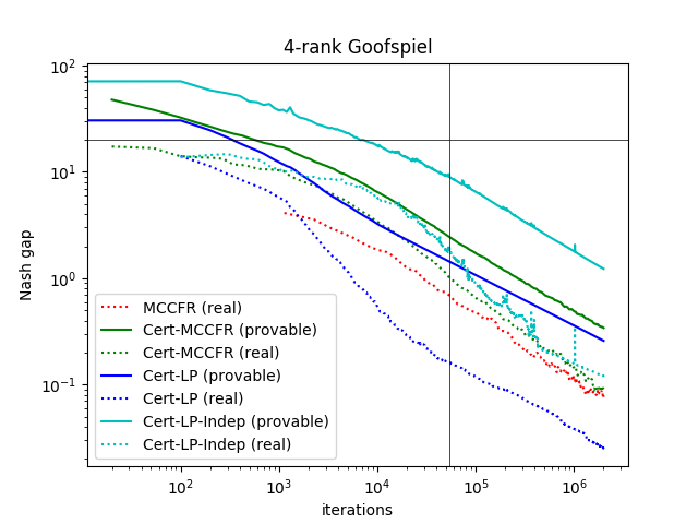
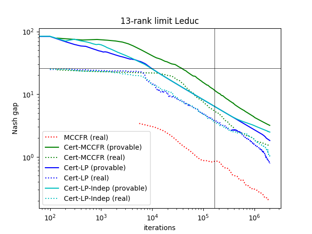
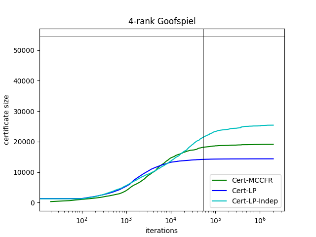
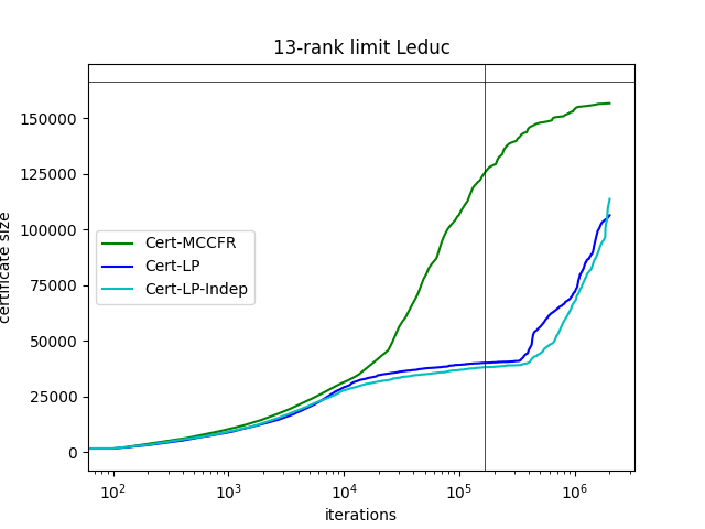
Figure 1: Convergence of Algorithm  and Algorithm  in 4-rank Goofspiel and 13-card limit Leduc. To be consistent with the other algorithms, one “iteration” of MCCFR consists of one accepted loss vector per player. For the other algorithms, one “iteration” is one playthrough. In all cases, we show both the provable equilibrium gap $\hat{\beta}^{*t}(\sigma^{t})-\hat{\alpha}^{*t}(\sigma^{t})$ and the true equilibrium gap $\beta^{*t}(\sigma^{t})-\alpha^{*t}(\sigma^{t})$. The exception is MCCFR, which on its own does not give provable equilibrium gaps in the same way. The horizontal line in the Nash gap graphs is at the game’s reward range (Goofspiel has reward range $[-10,10]$ and 13-rank Leduc has $[-13,13]$, so the lines are at $20$ and $26$, respectively). The vertical line in both graphs is at the number of nodes in the game (Goofspiel has 54,421 nodes and 13-rank Leduc has 166,366).

	Sampling-limited	Compute-limited
Unknown nature distributions	Algorithm  with LP solver	Algorithm  with a CFR variant (e.g., outcome-sampling MCCFR)
Known nature distributions	Algorithm 6.7 of Zhang and Sandholm (2020)

Table 1: Algorithms we suggest by use case in two-player zero-sum games. Sampling-limited means that the black-box game simulator is relatively slow or expensive compared to solving the pseudogames. Compute-limited means that the simulator is fast or cheap compared to solving the pseudogames. In general-sum games, only Algorithm  is usable.

Annoyingly, it is not the case in general that $\varepsilon_{i,t}=\tilde{O}(N_{t}/\sqrt{t})$. A counterexample is provided in the appendix. Intuitively, the reason is that, for a fixed strategy $\sigma$, the upper bound $\hat{\beta}^{t}(\sigma)$ is not a monotonically nonincreasing function of $t$; indeed, for strategies $\sigma$ that are not sampled very frequently, $\hat{\beta}^{t}(\sigma)$ may fluctuate by large amounts even when $t$ is large. However, the nonmonotonicity of $\hat{\beta}^{t}$ is, in some sense, necessary to achieve the high-probability correctness guarantee. If $\hat{\beta}^{t}$ does not increase over time, then the probability that it is an incorrect bound remains constant, rather than decreasing polynomially with time as would be desired.

To study the convergence rate of Algorithm , then, we will instead analyze the quantity

$$\bar{\varepsilon}_{i,T} =\max_{\sigma_{i}}\frac{1}{T}\sum_{t=1}^{T}\quantity[\hat{\beta}^{t}_{i}(\sigma_{i},\sigma^{t}_{-i})-\hat{\alpha}^{t}_{i}(\sigma^{t})]+O\quantity(\frac{1}{\sqrt{T}})$$ (7.3)

$$=\frac{1}{T}\quantity[R_{i,T}+U_{i,T}]+O\quantity(\frac{1}{\sqrt{T}})$$ (7.4)

where the $O$ hides only an absolute constant. This quantity is identical to $\varepsilon_{i,t}$ except that it uses $\hat{\beta}^{t}_{i}$ with $\sigma^{t}_{-i}$ instead of $\hat{\beta}^{T}_{i}$ to match the regret term, and has an extra error term added.

Proposition 7.5.

With probability $1-O(1/\sqrt{T})$, $\bar{\varepsilon}_{i,T}$ is an actual equilibrium gap bound.

By Theorem 5.6, $U_{T}=\tilde{O}(N_{T}\sqrt{T})$. Thus, this theorem matches the worst-case convergence of any algorithm with regret $\tilde{O}(N_{T}/\sqrt{T})$, up to a logarithmic factor. For example, using CFR and variants thereof matches the bound of Corollary 6.5 with iterates that are linear time in the size of the pseudogame. With MCCFR, the iterates can be made even faster, and due to Farina, Kroer, and Sandholm (2020), even outcome-sampling MCCFR can be used without breaking the $\tilde{O}(N_{T}/\sqrt{T})$ runtime bound.

Unfortunately, there is a further problem. It is often unwieldy to compute $\bar{\varepsilon}_{i,T}$. For example, if using outcome-sampling MCCFR, one may not even have access to the true bounds $\hat{\beta}^{t}(\cdot,\sigma^{t}_{-i})$ (and similar for $\alpha$) but only stochastic estimates $\tilde{\beta}^{t}(\cdot,\tilde{\sigma}^{t}_{-i})$ with the correct conditional expectation (Farina, Kroer, and Sandholm 2020). In that case, the stochastic estimate may be used as a substitute to create a stochastic equilibrium gap bound

$$\tilde{\varepsilon}_{i,T} =\max_{\sigma_{i}}\frac{1}{T}\!\sum_{t=1}^{T}\!\quantity[\tilde{\beta}^{t}_{i}(\sigma_{i},\sigma^{t}_{-i})-\tilde{\alpha}^{t}_{i}(\sigma^{t})]+O\quantity(\!M\sqrt{\frac{1}{T}\log T})$$ (7.6)

where $M$ is a bound on the norm of the estimates; i.e., $\absolutevalue{\tilde{\beta}^{t}_{i}(\sigma_{i},\tilde{\sigma}^{t}_{i})-\tilde{\beta}^{t}_{i}(\sigma^{\prime}_{i},\tilde{\sigma}^{t}_{i})}\leq M$ for every pair of strategies $\sigma_{i},\sigma_{i}^{\prime}$. As discussed by Farina, Kroer, and Sandholm (2020), with a uniform sampling vector, we can achieve $M\leq N_{T}$.

Proposition 7.7.

With probability $1-1/T$, for every time $T$ and player $i$, we have $\tilde{\varepsilon}_{i,T}\geq\bar{\varepsilon}_{i,T}$.

Thus, in particular, we have:

Corollary 7.8.

$\varepsilon^{*}_{i,T}:=\min(\varepsilon_{i,T},\tilde{\varepsilon}_{i,T})=\tilde{O}(N_{T}/\sqrt{T})$ is an equilibrium gap bound with probability $1-O(1/\sqrt{T})$.

This is the desired result. In practice, $\tilde{\varepsilon}_{i,T}$ is trivial until $T=\Omega(N_{T}^{2})$, and $\varepsilon_{i,T}$ is almost always a better bound. Thus, in our experiments, we use only $\varepsilon_{i,T}$. For this reason and for clarity, we have not bothered to specify the constants in the big-$O$s. Nevertheless, it is desirable theoretically to be able to define a quantity $\varepsilon^{*}_{i,T}$ that has both $\tilde{O}(N_{T}/\sqrt{T})$ convergence and (high-probability) correctness. As before, the correctness probability can be raised to any inverse-polynomial function of $T$ by a suitable change to Equation 5.2.

As an equilibrium-finding algorithm, Algorithm  is a “weaker” version of just running the underlying regret minimizers on the full game: instead of each regret minimizer getting access to the true losses, they only get access to an upper bound. However, its main advantage over regret minimization is, as before, its ability to give a equilibrium gap bound that can be computed without full knowledge of the remainder of the game or exact nature action probabilities.

Finally, Algorithm  has an unintuitive property.

Warning 7.9.

If $\mathcal{A}_{i}$ are stochastic regret minimizers (e.g. MCCFR), instead of submitting $-\hat{\beta}^{t}_{i}(\cdot,\sigma^{t}_{-i})$, it may be tempting to submit a noisy (sampled) version of $-\beta^{t}_{i}(\cdot,\sigma^{t}_{-i})$. Then the actual equilibrium gap $\beta^{*t}_{i}(\bar{\sigma}_{-i}^{t})-\alpha^{t}_{i}(\bar{\sigma}^{t})$ will converge, but the provable equilibrium gap $\bar{\varepsilon}_{i,t}$ may not. A counterexample is provided in the appendix.

7.4 The Case of Known Nature Probabilities: MCCFR Without Uniform Sampling

If the nature probabilities are assumed to be known exactly, 7.9 does not apply, since the actual bounds $(\alpha^{t},\beta^{t})$ and the sampled bounds $(\hat{\alpha}^{t},\hat{\beta}^{t})$ are the same. Even in this case, Algorithm  is still noteworthy: if we run it with outcome-sampling MCCFR, the result is an MCCFR-like algorithm (i.e., an equilibrium finder in the black-box case) that operates without an a-priori “uniform sampling strategy”. Indeed, the iterations only require a uniform sampling strategy over the current pseudogame, not the full game!

That algorithm is not quite a regret minimizer in the usual sense: its convergence rate depends on the uncertainty of the sampling method, and is tied to the fact that the sampling in Line 6 of Algorithm  uses the current strategy.

8 Experiments

We conducted experiments on two common benchmarks:

1. $k$-rank Goofspiel. At each time $t=1,\dots,k$, both players simultaneously place a bid for a prize. The prizes have values $1,\dots,k$, and are randomly shuffled. The valid bids are also $1,\dots,k$, each of which must be used exactly once during the game. The higher bid wins the prize; in case of a tie, the prize is split. The winner of each round is made public, but the bids are not. Our experiments use $k=4$.

2. $k$-rank heads-up limit Leduc poker (Southey et al. 2005), a small two-player variant of poker played with one hole card per player and one community card. Our experiments use a full range of poker ranks $(k=13)$.

We tested four algorithm variants. Except in the last case, which we will describe, all certificate-finding algorithms assume that the nature distributions are independent of player actions. In Goofspiel, we assume further that the nature distributions are independent of past nature actions, which is true (nature always plays uniformly at random).

1. MCCFR with outcome sampling (OS-MCCFR) (Lanctot et al. 2009) (MCCFR). This algorithm requires the game tree to be fully expanded, and does not give a (nontrivial) certificate. However, it does give a benchmark for actual equilibrium gap convergence.

2. Algorithm  with OS-MCCFR as the regret minimizer (Cert-MCCFR).

3. Algorithm , with LP for the game solves (Cert-LP). Since the LP solves are relatively expensive, we only recompute the LP solution every $100$ playthroughs sampled. This does not change the asymptotic performance of the algorithm. We use Gurobi v9.0.0 (Gurobi Optimization, LLC 2019) as the LP solver.

4. Algorithm , except with no assumptions on relationships between nature distributions (Cert-LP-Indep).

Footnote 5 shows the results. As expected, all the algorithms show a long-term convergence rate of roughly $\tilde{\Theta}(1/\sqrt{t})$. All certificate-finding algorithms find nontrivial provable certificates with fewer samples than it would take to expand the whole game tree, showing the efficacy of our method.

9 Conclusion and Future Research

We developed algorithms that construct high-probability certificates in games with only black-box access. Our method can be used with either an exact game solver (e.g., LP solver) as a subroutine or a regret minimizer such as MCCFR. Table 1 shows which algorithm we recommend based on the use case. As a side effect, we developed an MCCFR-like model-free equilibrium-finding algorithm that converges at rate $O(\sqrt{\log(t)/t})$, and does not require a lower-bounded sampling vector. We are, to our knowledge, the first to obtain this result. Our experiments show that our algorithms produce nontrivial certificates with very few samples.

This work opens many avenues for future research.

1. Is there a “cleaner” way to fix the problem introduced in Section 7.3? For example, a different confidence sequence may fix the problem, or it could be the case that $\varepsilon_{i,T}$ is small for most times $t$ (or even only a constant fraction), which would show that $\min_{t\leq T}\varepsilon_{i,T}=\tilde{O}(1/\sqrt{T})$, matching Corollary 6.5.

2. Is it possible to adapt Algorithm  to work with a generic extensive-form iterative game solver, for example, first-order methods such as EGT (Hoda et al. 2010; Kroer, Farina, and Sandholm 2018)?

3. In many practical games, there are nature nodes $h$ for which, under a particular profile $\sigma$, every child of $h$ has similar utility: the range of utilities of the children of $h$ under $\sigma$ is far smaller than $[\alpha(h\to*),\beta(h\to*)]$. Is it possible to incorporate this sort of information into the confidence-sequence pseudogames without losing perfect recall (which is needed for efficient solving)?

Appendix A Proofs of Theorems

A.1 Theorem 5.3

Lemma A.1.

Fix a player $i$ and chance node $h$. With probability at least $1-2/t^{2}Cn$, for any assignment $u:\operatorname{Children}(h)\to[\alpha,\beta]$ of utilities, we have

$$\absolutevalue{\operatorname*{\mathbb{E}}_{a\sim\sigma_{0}|h}u(ha)-\operatorname*{\mathbb{E}}_{a\sim\hat{\sigma}_{0}|h}u(ha)}\leq(\beta-\alpha)\rho(h).$$ (A.2)

Proof.

If $\rho=1$ the claim is trivial, so assume $\rho<1$. The desired error term is a convex function of $u$, so we need only prove the theorem for $u:\operatorname{Children}(h)\to\{\alpha,\beta\}$. By definition, $\hat{\sigma}_{0}|h$ was created by sampling $t(h)$ times. Thus, by Hoeffding, we have

$$\Pr[\absolutevalue{\operatorname*{\mathbb{E}}_{a\sim\sigma_{0}|h}u(ha)-\operatorname*{\mathbb{E}}_{a\sim\hat{\sigma}_{0}|h}u(ha)}\geq(\beta-\alpha)\rho] \leq 2\exp(-2t(h)\rho(h)^{2})$$ (A.3)

$$=2\exp(-\absolutevalue{A_{h}}\log 2-\log t^{2}Cn)$$ (A.4)

$$=\frac{2^{1-\absolutevalue{A(h)}}}{t^{2}Cn}$$ (A.5)

Taking a union bound over the $2^{|A_{h}|}$ choices of $u$ completes the proof. ∎

Thus, by a union bound, with probability $1-2/t^{2}$, the above lemma is true for every player and chance node. Condition on this event, and take any player $i$ and any profile $\sigma$. For notation, let $\hat{\sigma}$ be the strategy profile in which chance plays according to $\hat{\sigma}_{0}$ and the players play according to $\sigma$.

Lemma A.6.

At every node $h$, we have the bounds $\hat{\alpha}_{i}(\sigma|h)\leq\alpha_{i}(\sigma|h)\leq\beta_{i}(\sigma|h)\leq\hat{\beta}_{i}(\sigma|h)$.

Proof.

By induction, leaves first. At the leaves, the lemma is trivial. Let $h$ be any internal node. Then we have

$$\hat{\alpha}_{i}(\sigma|h) =\operatorname*{\mathbb{E}}_{a\sim\hat{\sigma}_{i}|h}\hat{\alpha}_{i}(\sigma|ha)-\rho(h)\Delta_{i}(h\to*)$$ (A.7)

$$\leq\operatorname*{\mathbb{E}}_{a\sim\hat{\sigma}_{i}|h}\alpha_{i}(\sigma|ha)-\rho(h)\Delta_{i}(h\to*)$$ (A.8)

$$\leq\operatorname*{\mathbb{E}}_{a\sim\sigma_{i}|h}\alpha_{i}(\sigma|ha)$$ (A.9)

$$=\alpha_{i}(\sigma|h).$$ (A.10)

where the first two inequalities use, in order, the inductive hypothesis and the last lemma. An identical proof holds for $\beta$, and we are done. ∎

The theorem now follows by applying the above lemma with $h=\emptyset$.

A.2 Theorem 5.6

Assume WLOG there is only one player, and drop the subscript $i$ accordingly. Define the sampled cumulative uncertainty $\hat{U}_{T}$ as

$$\hat{U}_{T}:=\sum_{t=1}^{T}\hat{\Delta}^{t}(z_{t})$$ (A.11)

where $z_{t}$ is the last node in $\hat{G}^{t}$ reached during the play at time $t$. By linearity of expectation, we have $\operatorname*{\mathbb{E}}\hat{U}_{T}=\operatorname*{\mathbb{E}}U_{T}$. Define $\hat{U}_{K}^{\Delta}(h)$ to be the sampled regret at node $h$ after node $h$ is sampled $K$ times. Formally,

$$\hat{U}_{K}(h) :=\sum_{k=1}^{K}\hat{\Delta}^{t_{h,k}}(h\to z_{t_{h,k}})$$ (A.12)

where $t_{h,k}$ is the $k$th timestep on which $h$ was sampled. Conveniently, $\hat{U}_{K}(h)$ can be analyzed independently of the rest of the game. Our goal is to bound $\hat{U}_{T}=\hat{U}_{T}(\emptyset)$.

Let $N_{k}(h)$ be the number of descendants of $h$, including $h$ itself, at time $t_{h,k}$. Let $C_{k}(h)$ be the same, except only counting chance nodes. Let $\rho_{k}(h)$ be the value of $\rho(h)$ after $k$ samples at $h$. Once again, these quantities are independent of what happens outside the subgame rooted at $h$. We now prove a lemma, which has the theorem as the special case $h=\emptyset$.

Lemma A.13.

For every exploration policy $\mathcal{A}$, any node $h$ of $G$, and any time $K$, we have

$$\operatorname*{\mathbb{E}}\hat{U}_{K}(h)\leq 2C_{k}(h)\sqrt{2KM}+N_{K}(h).$$ (A.14)

Proof.

By induction on the nodes of the game tree, leaves first. For each child $ha$ of $h$, let $K_{a}$ be the number of times action $a$ has been sampled.

Base case. If $h$ is a leaf of $G$, then uncertainty at most $1$ will be incurred when the leaf is expanded for the first time.

Inductive case.

$$\operatorname*{\mathbb{E}}\hat{U}_{K}(h) \leq\Delta(h\to*)\quantity(1+2\sum_{k=1}^{K}\rho_{k}(h))+\sum_{a\in A_{h}}\operatorname*{\mathbb{E}}\hat{U}_{K_{a}}(ha)$$ (A.15)

$$\leq 1+2\sum_{k=1}^{K}\sqrt{\frac{M}{2k}}+\sum_{a\in A_{h}}\quantity[C_{K_{a}}(ha)\sqrt{2K_{a}M}+N_{K_{a}}(ha).]$$ (A.16)

$$\leq 2C_{K}(h)\sqrt{2KM}+N_{K}(h)$$ (A.17)

where the three terms come from:

1. a regret of at most $1$, incurred when $h$ is first expanded,

2. the regret incurred at $h$ itself, if it is a chance node, and

3. the regret incurred at each child node. ∎

Once again, the theorem is the above lemma applied with $h=\emptyset$.

A.3 Proposition 6.2 and Proposition 7.2

Follow immediately from Theorem 5.3.

A.4 Proposition 6.4

Follows immediately from the definition of a pseudogame.

A.5 Proposition 7.5

Taking a union bound over times $t\geq\sqrt{T}$ in Theorem 5.3, we have that, with probability $1-O(1/\sqrt{T})$, $\hat{\beta}^{t}_{i}(\sigma_{i},\sigma^{t}_{-i})-\hat{\alpha}^{t}_{i}(\sigma^{t})\geq\beta^{t}(\sigma_{i},\sigma^{t}_{-i})-\alpha^{t}(\sigma^{t})$ for all $t\geq\sqrt{T}$. The bound follows.

A.6 Proposition 7.7

Identical to Theorem 1 of Farina, Kroer, and Sandholm (2020).

Appendix B Counterexamples

B.1 Rate of convergence of the upper bound in Proposition 7.2

Consider the following multi-armed bandit instance with two arms, formulated as a one-player game: the left arm gives loss $-K$ with probability $1/K$, and $0$ with probability $1-1/K$. The right arm gives loss $-1$ deterministically.

With probability $\Theta(1/K)$, the first $\Theta(K^{2})+1$ samples of the left arm give rewards exactly $(-K,-K,\dots,-K,0)$. Condition on this event.

After $\Theta(K^{2})$ samples of the left arm, its upper bound will be

$$-K+\Theta\quantity(K\sqrt{\frac{1}{K^{2}}\log T})=-K+\Theta(\sqrt{\log T})$$ (B.1)

The $\Theta(K^{2})+1$st sample will not happen until the upper bound exceeds at least $-1$, which only happens once $T>\exp(\Theta(K^{2}))$. Upon taking the $\Theta(K^{2})+1$st sample, the upper bound on the left arm’s utility will increase by $\Theta(1)$. But the reward range of this game is $[-K,0]$, so now taking any $K=o(\sqrt{T})$ completes the counterexample.

B.2 7.9

For example, consider the one-player multi-armed bandit case with two arms of differing utilities $u(L)<u(R)$. Then the following two statements are simultaneously true:

1. With MCCFR, with probability $1$, there will exist some time $T$ after which $L$ will no longer be played ever again.

2. $\hat{\beta}^{t}(L)$ will increase without bound if it is not played.

Thus, eventually, we will have $\hat{\beta}^{t}(L)>\hat{\beta}^{t}(R)$, after which time the provable equilibrium gap will always be at least their difference.

References

- Areyan Viqueira, Cousins, and Greenwald (2020) Areyan Viqueira, E.; Cousins, C.; and Greenwald, A. 2020. Improved Algorithms for Learning Equilibria in Simulation-Based Games. In Autonomous Agents and Multi-Agent Systems, 79–87.
- Auer, Cesa-Bianchi, and Fischer (2002) Auer, P.; Cesa-Bianchi, N.; and Fischer, P. 2002. Finite-time analysis of the multiarmed bandit problem. Machine learning 47(2-3): 235–256.
- Basilico and Gatti (2011) Basilico, N.; and Gatti, N. 2011. Automated Abstractions for Patrolling Security Games. In AAAI Conference on Artificial Intelligence (AAAI).
- Berner et al. (2019) Berner, C.; Brockman, G.; Chan, B.; Cheung, V.; Debiak, P.; Dennison, C.; Farhi, D.; Fischer, Q.; Hashme, S.; Hesse, C.; et al. 2019. Dota 2 with Large Scale Deep Reinforcement Learning. arXiv preprint arXiv:1912.06680 .
- Billings et al. (2003) Billings, D.; Burch, N.; Davidson, A.; Holte, R.; Schaeffer, J.; Schauenberg, T.; and Szafron, D. 2003. Approximating Game-Theoretic Optimal Strategies for Full-scale Poker. In Proceedings of the International Joint Conference on Artificial Intelligence (IJCAI).
- Bošanskỳ et al. (2014) Bošanskỳ, B.; Kiekintveld, C.; Lisý, V.; and Pěchouček, M. 2014. An Exact Double-Oracle Algorithm for Zero-Sum Extensive-Form Games with Imperfect Information. Journal of Artificial Intelligence Research 829–866.
- Bowling et al. (2015) Bowling, M.; Burch, N.; Johanson, M.; and Tammelin, O. 2015. Heads-up Limit Hold’em Poker is Solved. Science 347(6218).
- Brown and Sandholm (2015) Brown, N.; and Sandholm, T. 2015. Simultaneous Abstraction and Equilibrium Finding in Games. In Proceedings of the International Joint Conference on Artificial Intelligence (IJCAI).
- Brown and Sandholm (2017) Brown, N.; and Sandholm, T. 2017. Superhuman AI for heads-up no-limit poker: Libratus beats top professionals. Science eaao1733.
- Brown and Sandholm (2019a) Brown, N.; and Sandholm, T. 2019a. Solving imperfect-information games via discounted regret minimization. In AAAI Conference on Artificial Intelligence (AAAI).
- Brown and Sandholm (2019b) Brown, N.; and Sandholm, T. 2019b. Superhuman AI for multiplayer poker. Science 365(6456): 885–890.
- Čermák, Bošansky, and Lisý (2017) Čermák, J.; Bošansky, B.; and Lisý, V. 2017. An algorithm for constructing and solving imperfect recall abstractions of large extensive-form games. In Proceedings of the International Joint Conference on Artificial Intelligence (IJCAI), 936–942.
- Farina, Kroer, and Sandholm (2020) Farina, G.; Kroer, C.; and Sandholm, T. 2020. Stochastic regret minimization in extensive-form games. arXiv preprint arXiv:2002.08493 .
- Farina and Sandholm (2021) Farina, G.; and Sandholm, T. 2021. Model-Free Online Learning in Unknown Sequential Decision Making Problems and Games. In AAAI Conference on Artificial Intelligence.
- Farina, Schmucker, and Sandholm (2021) Farina, G.; Schmucker, R.; and Sandholm, T. 2021. Bandit Linear Optimization for Sequential Decision Making and Extensive-Form Games. In AAAI Conference on Artificial Intelligence.
- Gatti and Restelli (2011) Gatti, N.; and Restelli, M. 2011. Equilibrium approximation in simulation-based extensive-form games. In Autonomous Agents and Multi-Agent Systems, 199–206.
- Gilpin and Sandholm (2006) Gilpin, A.; and Sandholm, T. 2006. A Competitive Texas Hold’em Poker Player via Automated Abstraction and Real-Time Equilibrium Computation. In Proceedings of the National Conference on Artificial Intelligence (AAAI), 1007–1013.
- Gilpin and Sandholm (2007) Gilpin, A.; and Sandholm, T. 2007. Lossless Abstraction of Imperfect Information Games. Journal of the ACM 54(5).
- Gurobi Optimization, LLC (2019) Gurobi Optimization, LLC. 2019. Gurobi Optimizer Reference Manual.
- Hart, Nilsson, and Raphael (1968) Hart, P.; Nilsson, N.; and Raphael, B. 1968. A Formal Basis for the Heuristic Determination of Minimum Cost Paths. IEEE Transactions on Systems Science and Cybernetics 4(2): 100–107.
- Hart and Mas-Colell (2000) Hart, S.; and Mas-Colell, A. 2000. A Simple Adaptive Procedure Leading to Correlated Equilibrium. Econometrica 68: 1127–1150.
- Hoda et al. (2010) Hoda, S.; Gilpin, A.; Peña, J.; and Sandholm, T. 2010. Smoothing Techniques for Computing Nash Equilibria of Sequential Games. Mathematics of Operations Research 35(2).
- Koller, Megiddo, and von Stengel (1994) Koller, D.; Megiddo, N.; and von Stengel, B. 1994. Fast algorithms for finding randomized strategies in game trees. In Proceedings of the 26th ACM Symposium on Theory of Computing (STOC).
- Kroer, Farina, and Sandholm (2018) Kroer, C.; Farina, G.; and Sandholm, T. 2018. Solving Large Sequential Games with the Excessive Gap Technique. In Proceedings of the Annual Conference on Neural Information Processing Systems (NIPS).
- Kroer and Sandholm (2014) Kroer, C.; and Sandholm, T. 2014. Extensive-Form Game Abstraction With Bounds. In Proceedings of the ACM Conference on Economics and Computation (EC).
- Kroer and Sandholm (2015) Kroer, C.; and Sandholm, T. 2015. Discretization of Continuous Action Spaces in Extensive-Form Games. In International Conference on Autonomous Agents and Multi-Agent Systems (AAMAS).
- Kroer and Sandholm (2016) Kroer, C.; and Sandholm, T. 2016. Imperfect-Recall Abstractions with Bounds in Games. In Proceedings of the ACM Conference on Economics and Computation (EC).
- Kroer and Sandholm (2018) Kroer, C.; and Sandholm, T. 2018. A Unified Framework for Extensive-Form Game Abstraction with Bounds. In Proceedings of the Annual Conference on Neural Information Processing Systems (NIPS).
- Lanctot et al. (2012) Lanctot, M.; Gibson, R.; Burch, N.; Zinkevich, M.; and Bowling, M. 2012. No-Regret Learning in Extensive-Form Games with Imperfect Recall. In International Conference on Machine Learning (ICML).
- Lanctot et al. (2009) Lanctot, M.; Waugh, K.; Zinkevich, M.; and Bowling, M. 2009. Monte Carlo Sampling for Regret Minimization in Extensive Games. In Proceedings of the Annual Conference on Neural Information Processing Systems (NIPS).
- Lanctot et al. (2017) Lanctot, M.; Zambaldi, V.; Gruslys, A.; Lazaridou, A.; Tuyls, K.; Pérolat, J.; Silver, D.; and Graepel, T. 2017. A unified game-theoretic approach to multiagent reinforcement learning. In Proceedings of the Annual Conference on Neural Information Processing Systems (NIPS), 4190–4203.
- Moravčík et al. (2017) Moravčík, M.; Schmid, M.; Burch, N.; Lisý, V.; Morrill, D.; Bard, N.; Davis, T.; Waugh, K.; Johanson, M.; and Bowling, M. 2017. DeepStack: Expert-level artificial intelligence in heads-up no-limit poker. Science .
- Sandholm and Singh (2012) Sandholm, T.; and Singh, S. 2012. Lossy stochastic game abstraction with bounds. In Proceedings of the ACM Conference on Electronic Commerce (EC).
- Southey et al. (2005) Southey, F.; Bowling, M.; Larson, B.; Piccione, C.; Burch, N.; Billings, D.; and Rayner, C. 2005. Bayes’ Bluff: Opponent Modelling in Poker. In Proceedings of the 21st Annual Conference on Uncertainty in Artificial Intelligence (UAI).
- Tuyls et al. (2018) Tuyls, K.; Perolat, J.; Lanctot, M.; Leibo, J. Z.; and Graepel, T. 2018. A Generalised Method for Empirical Game Theoretic Analysis. In Proceedings of the 17th International Conference on Autonomous Agents and MultiAgent Systems, 77–85.
- Vinyals et al. (2019) Vinyals, O.; Babuschkin, I.; Czarnecki, W. M.; Mathieu, M.; Dudzik, A.; Chung, J.; Choi, D. H.; Powell, R.; Ewalds, T.; Georgiev, P.; et al. 2019. Grandmaster level in StarCraft II using multi-agent reinforcement learning. Nature 575(7782): 350–354.
- Wellman (2006) Wellman, M. 2006. Methods for Empirical Game-Theoretic Analysis (Extended Abstract). In Proceedings of the National Conference on Artificial Intelligence (AAAI), 1552–1555.
- Zhang and Sandholm (2020) Zhang, B. H.; and Sandholm, T. 2020. Small Nash Equilibrium Certificates in Very Large Games. arXiv preprint arXiv:2006.16387 .
- Zinkevich (2003) Zinkevich, M. 2003. Online Convex Programming and Generalized Infinitesimal Gradient Ascent. In International Conference on Machine Learning (ICML), 928–936. Washington, DC, USA.
- Zinkevich et al. (2007) Zinkevich, M.; Bowling, M.; Johanson, M.; and Piccione, C. 2007. Regret Minimization in Games with Incomplete Information. In Proceedings of the Annual Conference on Neural Information Processing Systems (NIPS).