A Scalable Real-Time Architecture for Neural Oscillation Detection and Phase-Specific Stimulation

Abstract

Oscillations in the local field potential (LFP) of the brain are key signatures of neural information processing. Perturbing these oscillations at specific phases in order to alter neural information processing is an area of active research. Existing systems for phase-specific brain stimulation typically either do not offer real-time timing guarantees (desktop computer based systems) or require extensive programming of vendor-specific equipment. This work presents a real-time detection system architecture that is platform-agnostic and that scales to thousands of recording channels, validated using a proof-of-concept microcontroller-based implementation.

I Introduction

Recording of electrical signals from neurons in human and animal brains is a well-established field[1]. Processing these signals reveals two related components: “spikes”, representing the firing of individual neurons near the pickup electrodes, and the “local field potential” (LFP), representing the aggregate activity of the larger population of neurons surrounding the electrode site[2]. Both of these signal components carry information: spikes via firing rate and timing[3][4] [5][6], and the LFP via the presence or absence of transient oscillations representing coherent activity of a large group of neurons[7][8] [9][10][11]. The relative timing of spikes with respect to LFP oscillation phase has also been shown to encode information[12][13] [6][14][15].

Artificial stimulation of human and animal brains (via electrical, optical, or other means) is also a field of active study[16][17] [18][19]. It has recently been shown that if LFP oscillations are present near a stimulation site, the timing of stimulation with respect to the LFP phase is important[20][21] [22][23]. In order to study this, it is necessary to perform “on-line” detection of transient LFP oscillations and to extract phase in real-time.

Existing experiments studying phase-specific stimulation can be divided into those that use a desktop computer to perform their signal processing[20][24] [25][21] and those which perform some or all of their signal processing on dedicated hardware[26][27]. Both types of system have signal processing latency that must be compensated for (typically 20-100 ms)[26][21] but desktop computer based systems usually have substantial random variation (jitter) in processing and communications latency (typically 5-10 ms)[21], which is avoided in systems that keep the stimulation trigger processing entirely in dedicated hardware.

Low-latency signal processing systems running on dedicated hardware may be implemented in software running on dedicated digital signal processing (DSP) platforms[26][28] or implemented using a field-programmable gate array (FPGA) tightly coupled to the recording system[27][29]. Signal processing on dedicated hardware is widely used for processing of neural signals but is typically implemented ad-hoc.

The goal of this work is to present and validate an open architecture for “on-line” LFP oscillation detection and for phase-aligned stimulation that is suitable for instantiation on conventional FPGA-based electrophysiology equipment and that is scalable to thousands of recording channels. The purpose of this architecture is to make it easier and faster to implement experiment-specific closed-loop stimulation systems (using FPGA-based equipment or using embedded software), as most of the implementation and debugging will already have been done.

II Background

II-A Electrophysiology Measurements

A diagram of a typical electrophysiology recording and stimulation setup is shown in Figure 1. One or more probes, typically containing multiple electrical contacts per probe, are inserted into the brain. A “headstage” and a recording controller amplify and digitize the analog signals and forward them to a host computer. Electrical stimulation is performed using either a dedicated controller and probes or auxiliary functions of the controller, headstage, and probes used for recording. Recording and stimulation are typically performed while the subject performs some consistently-structured activity.

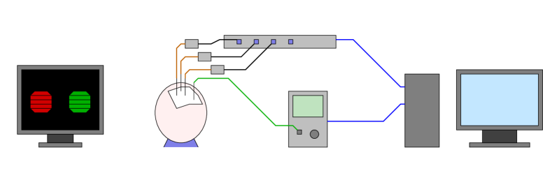
Figure 1: Typical electrophysiology recording and stimulation setup using wire probes or linear silicon probes. A recorder captures electrical signals from probes, which are processed by a control computer, which commands a stimulation controller.

A typical single-channel recorded waveform is shown in Figure 2[30]. Noteworthy features are spikes (sub-millisecond duration)[31][32], local field potential oscillations (typically 4-50 Hz and lasting for a small number of cycles[33]), and background noise (typically $\frac{1}{f^{2}}$ power-law noise at LFP frequencies[34][35]). Spiking and LFP oscillation patterns vary widely depending on the region of the brain being measured[36][37], and LFP oscillation duration (absolute and number of cycles) also depends strongly on the oscillation frequency[38]. At high frequencies (50-200 Hz), oscillations occur with durations of many cycles that are are modulated by co-occurring low-frequency oscillations[10].

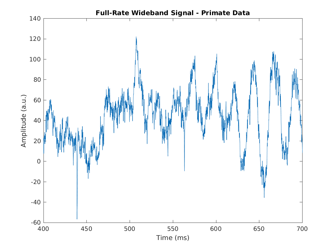
Figure 2: Typical wide-band-signal recorded from a primate brain using tungsten wire probes[30]. Noteworthy features in this signal are sub-millisecond spikes and 20-25 Hz oscillations.

A typical closed-loop phase-aligned stimulation setup based on a desktop computer is shown in Figure 3. Signals are acquired using the recording controller and processed using “on-line” algorithms that are intended to function in real-time. When a transient oscillation occurs and stimulation is commanded during the experiment, the desktop computer waits until the appropriate oscillation phase before commanding the stimulation controller to activate.

Figure 3: Data processing flow within a typical electrophysiology recording and stimulation setup using a desktop computer for phase-aligned stimulation. Acquired signals are band-pass filtered, and magnitude and phase are estimated either by feature extraction, template matching, or by using a windowed Hilbert transform. If a request for stimulation is queued, and an oscillation is occurring, stimulation is performed at the desired phase.

Typical “on-line” oscillation detection and characterization algorithms are variants of a widely-used “offline” algorithm. In this particular offline algorithm, the LFP frequency band of interest is isolated and the analytic signal is computed, with the imaginary component provided by the Hilbert transform of the band-pass-filtered signal. The analytic signal encodes the magnitude and phase of the original narrow-band signal[39][25]. Oscillation events are identified by looking for magnitude excursions, with $2\sigma$ or $3\sigma$ from baseline magnitude being typical[20][7] [26][5]. Oscillation phase at any given instant is taken to be the analytic signal phase at the time of interest. For ease of reference, this will be referred to as the “offline Hilbert algorithm”.

For “on-line” implementation, band-pass filtering is typically performed using a finite impulse response filter (FIR)[26]. Magnitude and phase may be extracted using template-fitting[20] using interpolation between peaks, troughs, and zero-crossings in the narrow-band signal[39][40]. Oscillation period may be estimated by using template fitting, by using the locations of peaks, troughs, and zero-crossings, or by using a filter bank with densely-spaced center frequencies and looking for the filter with the strongest response[26].

“Offline” algorithms for oscillation detection and parameterization are more varied[41], as they do not need to meet response time constraints and they can consider both the past and future signal around a point of interest. Typical approaches that do not use the Hilbert transform involve decomposing the signal using either a fixed dictionary such as Gabor wavelets[42] or an optimized dictionary via sparse coding approaches[43][44].

The desired goal for real-time closed-loop experiments is to detect local field potential oscillations while they are still happening (within 1-2 oscillation periods), and to accurately determine the oscillation phase so that phase-specific stimulation may be performed. The accuracy needed can be inferred from the number of phase bins used for spike-phase coding analyses; 4–10 phase bins are typical, with diminishing returns past 6 bins[5] [3]. This indicates that the full-width half-maximum of the phase error distribution should be 60 degrees or less.

II-B Signal Processing Hardware

Hardware-based signal processing of electrophysiology signals typically involves electrophysiology controllers that expose digital signal processors (DSPs) or field-programmable gate arrays (FPGAs) to the user. These are programmable (DSP) or configurable (FPGA) hardware devices capable of running specialized computing operations much faster than general-purpose microprocessors. User-supplied code is written to these DSP or FPGA components, which then becomes a part of the signal processing pipeline within these devices.

The performance metric that determines filtering and signal processing capability is the number of multiply-accumulate operations (MACs) that a given platform can perform per second. For a given number of channels, this determines the number of multiply-accumulate operations per channel per second, and for a given sampling rate, this determines the number of multiply-accumulate operations that may be performed per sample. The number of MAC operations available per sample is a design constraint for the implementation of signal processing pipelines.

A typical electrophysiology controller that exposes DSP features to the user is the Tucker-Davis RZ2 BioAmp Processor[28] (based on the SHARC series of DSP processors). For DSP-based systems, the number of MACs is usually equivalent to the number of floating point operations per second (FLOPS). The SHARC DSP processors used by Tucker-Davis can perform 2.4 GFLOPS per core (at 400 MHz), for an aggregate maximum processing power of about 77 GMAC/sec (8 quad-core boards). These processors are typically connected to digitizing pre-amplifiers supplying up to 256 channels[45], resulting in a budget of 300 MMAC/sec$\cdot$channel.

Typical electrophysiology controllers that expose FPGA features to the user are the Open Ephys acquisition board[46][47] and the related Intan RHD recording controller[48] (both based on the Xilinx Spartan 6 LX45 FPGA), and the NeuraLynx Hardware Processing Platform expansion board[29] (based on the Xilinx Zynq 7045 SoC which integrates a Kintex 7 FPGA). For Xilinx-family FPGA-based systems, the number of MACs per second is determined by the number of “digital signal processing slices” and the rate at which these slices maybe clocked. The XC6LX45 chip used in the Open Ephys and Intan controllers provides 5.8 GMAC/sec (58 units clocked at 100 MHz); some of this capacity is used for the controller’s built-in filtering operations. These controllers can acquire data from up to 1024 recording channels, resulting in a budget of 5.8 MMAC/sec$\cdot$channel, minus overhead for built-in filtering. The XC7Z045 chip used in the NeuraLynx processing board provides 900 GMAC/sec (900 units clocked at 1 GHz), all of which is available for signal processing. The controller in which this board is installed can acquire data from up to 512 recording channels, resulting in a budget of 1.76 GMAC/sec$\cdot$channel.

While these examples are not exhaustive, it is reasonable to assume a processing budget of at least 3 MMAC/sec per channel, with up to 2 GMAC/sec per channel available in systems with more hardware resources available. LFP signal processing is typically performed at 1 ksps, with signals acquired at 25 ksps–40 ksps[26].

III Implementation

III-A Architecture

A block diagram of the oscillation detection architecture is shown in Figure 4. Full-rate data is passed through an anti-aliasing filter and downsampled. Downsampled data is passed through a filter bank that performs band-pass filtering, and an approximation of its instantaneous magnitude and phase is extracted. Oscillation detection in each band is performed by magnitude thresholding, event detection logic building event triggers.

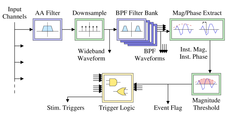
Figure 4: Top-level oscillation detector architecture. Input signals are downsampled and band-pass filtered; instantaneous magnitude, frequency, and phase are then estimated. Oscillations are detected by magnitude thresholding, and stimulation triggers are generated based on oscillation detector outputs.

Several features of this architecture require detailed discussion: Filter implementation and the associated corrections for delays introduced by the filters; estimation of instantaneous magnitude, frequency, and phase; and event detection logic.

Anti-aliasing filtering and band-pass filtering are implemented using either finite impulse response filters (FIR filters) or infinite impulse response filters (IIR filters). Both of these introduce delay (a fixed delay for FIR filters, and a frequency-dependent delay for IIR filters). Time shifts are added to the phase estimate to correct for these delays. For finite impulse response filters, a fixed time shift is used; for infinite impulse response filters, the time shift is read from a lookup table indexed by the estimated instantaneous frequency. Errors in the frequency estimate result in errors in the phase shift estimate when using lookup table time shifts.

Estimates of instantaneous magnitude, frequency, and phase are obtained using time-domain methods. The baseline implementation used for this architecture uses peaks and troughs to estimate magnitude and zero-crossings to estimate phase[39]. Potential extensions include using flank midpoints to estimate phase[40] and using complex demodulation to estimate magnitude and phase[39], with components provided by in-phase and quadrature FIR filters in the band-pass filter bank.

Transient oscillation detection is performed using magnitude thresholding. Two thresholds are used: a higher “turn-on” threshold and a lower “turn-off’ threshold, providing hysteresis. Threshold comparator inputs may optionally be required to remain high or low for a certain time interval before changing state, to suppress “glitching” in comparator output. The intention is to provide a number of tuning methods sufficient to suppress spurious detections and “drop-outs” in noisy input, despite the character of this input varying widely between use-cases.

Stimulation trigger generation logic also varies with use-case. The baseline implementation used for this architecture links stimulation triggers to the outputs of individual event detectors. A planned extension is contingent triggering based on the output of multiple detectors, to cover use-cases where triggering is to be performed during co-occurring oscillations[10]. Triggering is constrained to a user-specified time window and maximum number of trigger assertions, to ensure that spurious event detections do not result in unsafe stimulation.

The individual signal processing blocks in this architecture were implemented as modules, with the intention being that application-specific signal processing architectures would be built by assembling modules with a minimum of new code needed. While the desired output from a system implementation is typically the stimulation trigger flags, the outputs of all signal processing modules are potentially accessible for debugging or diagnostic purposes.

Each of the signal processing modules was implemented in C++ and in Matlab, with FPGA-based implementations in development. The intention is to allow rapid prototyping via Matlab, embedded software and workstation-based implementations via C++, and full-scale hardware implementations via hardware description languages, with confidence that all three types of implementation would produce comparable output if given the same input. As FPGA implementation is the end-goal, the C++ modules are written to operate in a pipelined manner on a sample-by-sample basis to facilitate translation to hardware and cycle-by-cycle comparison with hardware.

Three closed-loop systems were assembled as reference implementations: One off-line Matlab-based implementation, one off-line C++-based running on a desktop workstation (the “Burst Station” implementation), and one on-line embedded C++ implementation running on a proof-of-concept microcontroller-based hardware (the “Burst Box” implementation). The Matlab implementation was used to verify that the architecture is conceptually sound; it was not otherwise resource-constrained (no memory or processing time limits, double-precision floating-point arithmetic). The workstation-based “Burst Station” C++ implementation was used to verify that the architecture’s integer-arithmetic implementation produced output acceptably close to that of the Matlab implementation. While the workstation-based implementation was not explicitly memory-constrained, care was taken to keep internal structure sizes small enough to be instantiated on FPGAs. The embedded “Burst Box” prototype was used to verify that the architecture was capable of performing closed-loop stimulation in real-time with limited memory and a limited amount of processing power available.

Module library code and the closed-loop system reference implementations were made freely available under an open-source license[49].

III-B Workstation Implementation

The workstation-based C++ implementation (the “Burst Station”) was run as an “off-line” system: input signals were loaded from disk, rather than captured in real-time. The “Burst Station” was implemented as a test-bed for detection architectures and as a prototyping tool for building embedded implementations. The output of the “Burst Station” for a given input signal should be identical to the output of an “on-line” embedded system running with the same configuration.

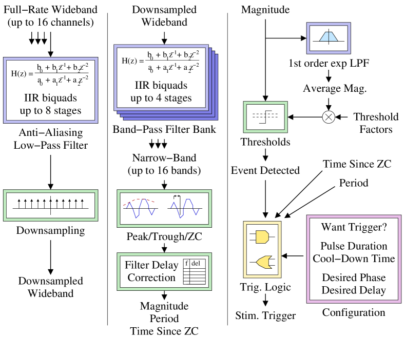
Figure 5: Workstation-based implementation of the oscillation detector architecture. Input is passed through an anti-aliasing filter, downsampled, and then passed through widely-spaced or densely-spaced band-pass filters. For densely-spaced filters, “winner-take-all” logic identifies the filter with the strongest response. Running estimates of magnitude, phase, and period are made using peak-and-trough estimators. Two-level magnitude thresholding is used to detect transient oscillation events. If an event is detected, phase- or delay-aligned stimulation trigger pulses may be generated.

A block diagram of the “Burst Station” signal processing architecture is shown in Figure 5. Input is passed through an anti-aliasing filter (FIR or IIR) and then downsampled. The anti-aliasing filter has a corner frequency higher than the highest LFP band edge of interest and at least 5 times lower than the Nyquist frequency, to ensure adequate suppression of aliased components. The downsampled signal is then passed through a bank of band-pass filters. The pass bands of these filters may be widely spaced and non-overlapping or densely-spaced and highly-overlapping. In the non-overlapping case, any given transient oscillation is expected to show up in a single filter’s output. In the highly-overlapping case, any given transient oscillation is expected to show up in multiple filters’ outputs, and a winner-take-all decision is performed to identify the filter with the strongest response. This filter’s center frequency is taken to be the nominal frequency of the event.

A running estimate of signal magnitude, phase, and period is produced for each band-pass filter’s output by peak, trough, and zero-crossing estimators. Oscillation detection is performed using a two-threshold scheme (activating when magnitude reaches the higher threshold and deactivating when magnitude falls below the lower threshold). Activation after exceeding the rising threshold is delayed by a fixed number of samples (typically half a period at the mid-band frequency), to allow the estimate of the signal’s period to stabilize before the oscillation detection signal is asserted. The running estimate of phase has a correction applied to compensate for the delay of the filter. For FIR filters, this delay is fixed at design-time. For IIR filters, this delay depends on frequency, and is fetched from a lookup table indexed by the detected period. The detected period used for this indexing may be either the running estimate or (for highly-overlapping filters) the center frequency of the band identified by the winner-take-all decision.

When an oscillation is detected, stimulation trigger logic compares the running estimate of the signal phase, delay since rising zero-crossing, or delay since falling zero-crossing against a user-specified target value. When the running estimate crosses the target value, a trigger pulse is generated. To ensure safety, a “quota” system is implemented, capping the number of trigger pulses delivered to some user-specified maximum. An activity time-out is also specified (typically several seconds); after this time-out has expired, oscillations no longer generate stimulation trigger pulses.

Calculations within the “Burst Station” were performed using 32-bit integer arithmetic with a signal range of 14 bits (to ensure sufficient head-room during multiply-accumulate operations). The C++ library’s IIR filters were implemented as cascaded biquad filters with Direct Form I implementation, given by Equation 1. The $a_{0}$ biquad denominator coefficient was required to be a power of two, so that the $\frac{1}{a_{0}}$ operation could be performed as a bit-shift.

$$y[n]=\left(\frac{1}{a_{0}}\right)(b_{0}x[n]+b_{1}x[n-1]+b_{2}x[n-2]\\ -a_{1}y[n-1]-a_{2}y[n-2])$$ (1)

III-C Embedded Microcontroller Implementation

The embedded microcontroller-based implementation (the “Burst Box”) was run as an “on-line” system: input signals were captured in real-time from analog input connectors, and stimulation trigger pulses were emitted as TTL signals. Physical connections were via BNC connectors, for compatibility with electrophysiology equipment. The “Burst Box” was implemented as a proof-of-concept prototype that can be used in as part of a functioning electrophysiology experiment.

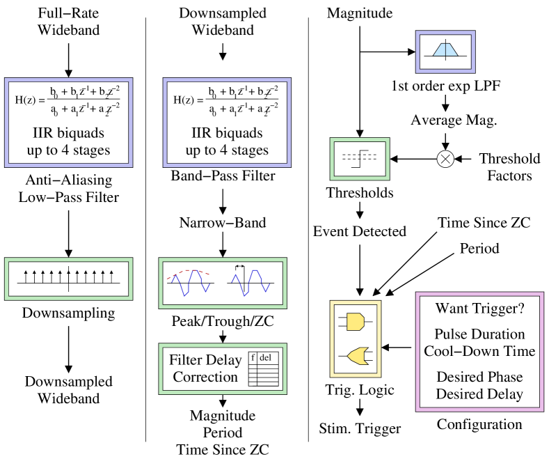
Figure 6: Microcontroller-based implementation of the oscillation detector architecture. Input is passed through an anti-aliasing filter, downsampled, and then passed through a band-pass filter. Running estimates of magnitude, phase, and period are made using a peak-and-trough estimator. Two-level magnitude thresholding is used to detect transient oscillation events. If an event is detected, phase- or delay-aligned stimulation trigger pulses may be generated.

A block diagram of the “Burst Box” signal processing architecture is shown in Figure 6. This is a subset of the “Burst Station” workstation-based implementation’s architecture described in Section III-B. Processing is restricted to one channel and one frequency band. Input is passed through a hardware anti-aliasing filter and a software anti-aliasing filter, downsampled, and then passed through a band-pass filter. Anti-aliasing and band-pass filters are implemented as infinite impulse response filters (IIR), to minimize processing load.

As with the “Burst Station”, a running estimate of the magnitude, phase, and period of the band-pass-filtered signal is produced using a peak, trough, and zero-crossing estimator. Oscillation detection is performed using a two-threshold scheme (activating when magnitude reaches the higher threshold and deactivating when magnitude falls below the lower threshold). Activation after exceeding the rising threshold is delayed by a fixed number of samples (typically half a period at the mid-band frequency), to allow the estimate of the signal’s period to stabilize before the oscillation detection signal is asserted. The running estimate of phase has a correction applied to compensate for the delay of the IIR filter. As this delay depends on frequency, the correction is fetched from a lookup table indexed by the estimated period.

As with the “Burst Station”, when an oscillation is detected, stimulation trigger logic compares the running estimate of the signal phase, delay since rising zero-crossing, or delay since falling zero-crossing against a user-specified target value. When the running estimate crosses the target value, a trigger pulse is generated. To ensure safety, the number of trigger pulses that may be generated and the time window within which they may be generated are both limited; oscillations that are detected after this pulse quota has been exceeded or after the time-out window has expired do not generate stimulation trigger pulses.

A block diagram of the firmware for the “Burst Box” is shown in Figure 7. Three concurrent execution threads are running: an interrupt service thread, which handles events that must occur with every real-time clock tick and complete within that timeslice; a high-priority polling thread, which is woken up by the real-time clock (preempting low-priority polling) but which may take multiple timeslices to complete; and a low-priority polling thread, which handles operations which do not require timing guarantees.

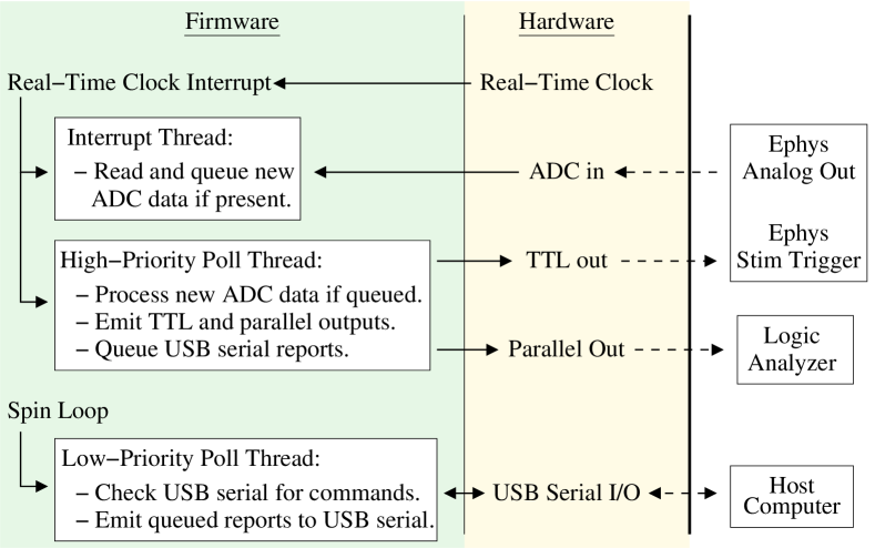
Figure 7: Embedded oscillation detector firmware architecture. Analog to digital conversion is handled once per real-time-clock tick. Signal processing is handled in a high-priority polling loop; this reads new ADC data if present, generates TTL output and diagnostic parallel output, and queues USB reports. A low-priority polling thread reads USB commands from the host computer and sends reports to the host computer.

The physical implementation of the “Burst Box” proof-of-concept prototype is shown in Figure 8. The microcontroller used is an Atmel ATmega2560 (8-bit, running at 16 MHz, with 8 kiB of SRAM); DSP performance was benchmarked at approximately 100 kMAC/sec with 32-bit operands. “Full-rate” signals are sampled at 2.5 ksps using an external analog to digital converter and a hardware anti-aliasing filter, and then downsampled to 500 sps internally (the “DSP rate”) after the application of a digital anti-aliasing filter. At 200 MAC/sample, this represents a worst-case lower bound to the processing budget available in real implementations.

Figure 8: Physical implementation of the microcontroller-based oscillation detector (“Burst Box”). Analog filters and the analog-to-digital converter are on the left; TTL outputs are on the right. The middle board is a break-out board, with the microcontroller board underneath it.

A diagram of the hardware implementation of the “Burst Box” is shown in Figure 9. There is hardware support for up to 4 input channels and 4 TTL outputs. The hardware anti-aliasing filter in this prototype was implemented as an RC ladder filter for simplicity and to avoid any possibility of resonance from inductive components, with the tradeoff of having poor roll-off compared to a Butterworth implementation. For debugging purposes, the system can be configured to bypass the external analog-to-digital converter and filters and use the microcontroller’s internal analog-to-digital converter at 500 sps without anti-aliasing.

Figure 9: Block diagram of the “Burst Box” hardware implementation. Input channels are level-shifted and filtered using a passive analog network before being digitized by the external analog to digital converter. Analog input may optionally be fed to the microcontroller’s internal analog to digital converter without filtering.

IV Validation

IV-A Datasets

Two datasets were used for testing and validation of oscillation detector implementations. The first (the “synthetic” dataset) consisted of 5 minutes of $\frac{1}{f^{2}}$ noise (“red noise”) with tones overlaid. Tones had weak frequency chirping and amplitude ramping (less than 5% and 10% respectively), with cosine roll-off (Tukey window roll-off), and durations of 3–5 periods between midpoints of the roll-off flanks. Tones had a signal-to-noise ratio of 20 dB with respect to in-band noise; frequency bands used for noise calculations are shown in Table I. The “red noise” spectrum spanned from 2–200 Hz, with power concentrated at lower frequencies, so per-band adjustment of tone amplitude was necessary in order to have consistent signal-to-noise ratios.

TABLE I: Synthetic Dataset Noise Bands

Freq (Hz)	4–7	7–12	12–21	21–36	36–63	63–108
Band	theta	alpha	beta	gamma	gamma	gamma

The second dataset (“biological” dataset) consisted of a concatenated selection of recordings from a primate dataset[50]. The raw dataset consisted of “epochs” that were typically less than 10 seconds long, taken during individual task trials within one extended recording session. Signals from individual epochs were trimmed to time periods within the task that showed consistent activity with few electrical artifacts. Signals were evaluated on an epoch-by-epoch basis to reject records that contained artifacts within the trimming interval (typically large step transients caused by physical contact with equipment or 60 Hz tones coupled from nearby equipment). Remaining “clean” epochs were normalized to have consistent average power and were concatenated with an overlap of 0.5 s with linear interpolation between signals within the overlap interval. The intention was to produce an artifact-free signal of several minutes’ duration with biologically valid noise and oscillation features.

IV-B Test Procedure

Validation tests were intended to measure several things: the transfer function of the band-pass filters, the accuracy of magnitude and phase estimation with respect to the analytic signal’s magnitude and phase, and the timing accuracy of stimulation pulses with respect to the desired stimulation times (specific phases or specific delays after a rising or falling zero crossing). The goal is to demonstrate a closed-loop system with stimulation phase accuracy of $\pm 30^{\circ}$ or better (jitter full-width half-maximum of $60^{\circ}$ or less).

Testing of the “off-line” Matlab-based and workstation-based oscillation detectors was straightforward; both provide as output time series waveforms for all internal signals in their processing pipelines, with a common time reference between all signals. The challenge was to extract comparable information from the “on-line” embedded microcontroller-based implementation during real-time tests.

The physical setup for real-time testing is shown in Figure 10. Signal waveforms were converted to sound files and played back to the “Burst Box” prototype via computer audio output. Volume settings for playback were adjusted until the output amplitude was approximately 3 V peak-to-peak, as measured using an oscilloscope. The “Burst Box” is capable of providing monitoring streams of two signals (typically the band-pass filtered waveform and one other signal derived from it). Tests with a given input waveform were run repeatedly, capturing different output waveform pairs, and these output waveform pares were time-aligned using the band-pass filtered waveform as a reference (which should remain consistent between successive trials).

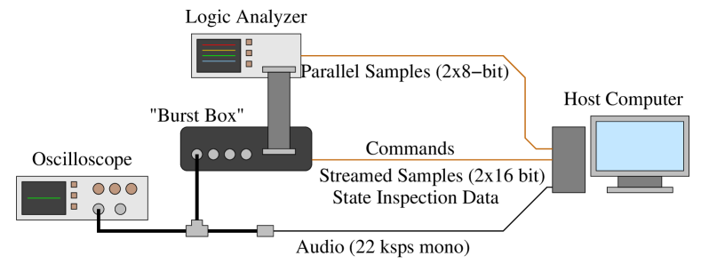
Figure 10: Physical setup for validation tests.

Signals streamed from the “Burst Box” could be read via two methods: parallel output via a logic header (8 bits per sample, precise timing and no dropped samples), and diagnostic output via the USB serial command interface (16 bits per sample, some dropped samples). Both capture methods were used. Unless otherwise indicated, the logic header output was used to generate plots.

Functionality exists for inspecting and modifying the internal state of the “Burst Box” using the serial command interface for single-stepped testing. While this would provide all of the desired signals with high fidelity, it was not practical to use for full-duration test signals, due to being far slower than real-time testing.

IV-C Filter Validation

The purpose of filter validation is to confirm that the integer math C++ implementations of the oscillation detector’s filters match the behavior of the Matlab implementation of the same filters. This tested by plotting the inferred filter transfer functions measured during functionality tests against the ideal transfer functions.

Filter gain, phase shift, phase delay, and group delay were characterized by taking the Fourier transform of the time-aligned input and output waveforms for each filter under test. Dividing spectrum elements gives the frequency-domain transfer function directly, per Equation 2. This is smoothed, to reduce artifacts due to noise, and the phase is unwrapped. The phase delay and group delay are then computed per Equations 3 and 4, respectively. The derivative of $\phi(\omega)$ is approximated by taking the first difference and performing additional smoothing.

$$\begin{split}H(\omega)&=\frac{\mathcal{F}\{y(t)\}}{\mathcal{F}\{x(t)\}}\\ G(\omega)&=||H(\omega)||\\ \phi(\omega)&=\mathrm{arg}(H(\omega))\end{split}$$ (2)

$$\tau_{\phi}(\omega)=-\frac{\phi(\omega)}{\omega}$$ (3)

$$\tau_{g}(\omega)=-\frac{d\phi(\omega)}{d\omega}$$ (4)

The band-pass IIR filter configurations used by the reference implementations are shown in Figure 11. These were Butterworth filters implemented as two-stage digital biquad filters (with second-order roll-off). The anti-aliasing filter (not shown) was a low-pass Butterworth filter implemented as a two-stage digital biquad filter with fourth-order roll-off.

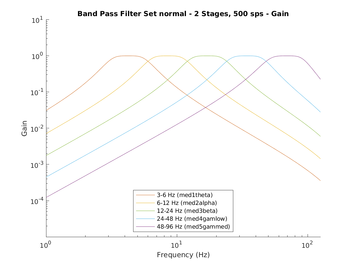
Figure 11: Designed transfer functions for infinite impulse response band-pass filters. These were Butterworth filters implemented as two-stage digital biquad filters with 2nd-order roll-off.

A representative plot of the designed and measured transfer functions for the “beta band” IIR filter is shown in Figure 12, using the “synthetic” dataset as the input signal. Within the regions of interest (blue in the plots), the designed and measured transfer functions are virtually identical. The same was observed in the measured transfer functions of IIR filters constructed for other bands, and for the anti-aliasing IIR filter. As a result, the filter implementation can be considered sound, and the Matlab models of the filters may be used as proxies for the real filter implementations without significant discrepancies expected.

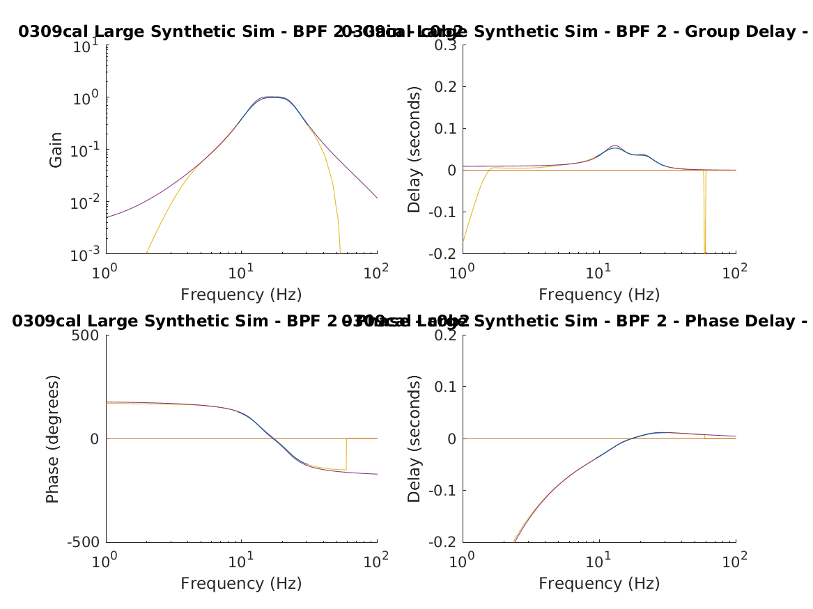
Figure 12: Designed and measured transfer functions for the beta band infinite impulse response filter. Upper left: gain response. Lower left: phase response. Upper right: group delay. Lower right: phase delay.

All causal filters introduce delay into the filtered signal. For FIR filters, this delay is constant, and for IIR filters, different frequency components are delayed by different amounts. To allow later processing stages to compensate for this, a calibration table of phase delay vs period was built. This is discussed in Section IV-F.

IV-D Magnitude and Phase Estimation

Instantaneous magnitude and phase were estimated by looking for zero-crossings in the band-pass-filtered waveform, inferring period and phase from those zero crossings, and taking the maximum or minimum value of the waveform between successive zero-crossings as the magnitude of the signal. Estimation accuracy was characterized by comparing the oscillation detector’s estimates of instantaneous magnitude, phase, and frequency (derived from period) to the instantaneous magnitude, phase, and (smoothed) frequency computed from the band-pass-filtered signal by using Hilbert transform to derive the imaginary component of the analytic signal.

Figure 13 shows a representative reconstruction of magnitude, phase, frequency, and waveform using the peak-trough-ZC feature extractor (blue) and using the analytic signal (orange) (beta band signal, IIR filters, “synthetic” dataset). Feature extractor reconstruction was performed in regions where the oscillation detector described in III-A indicated oscillation, and overlaid on top of the analytic signal plots. Regions where the analytic signal’s instantaneous magnitude is greater than twice the average magnitude are indicated in the plot for comparison.

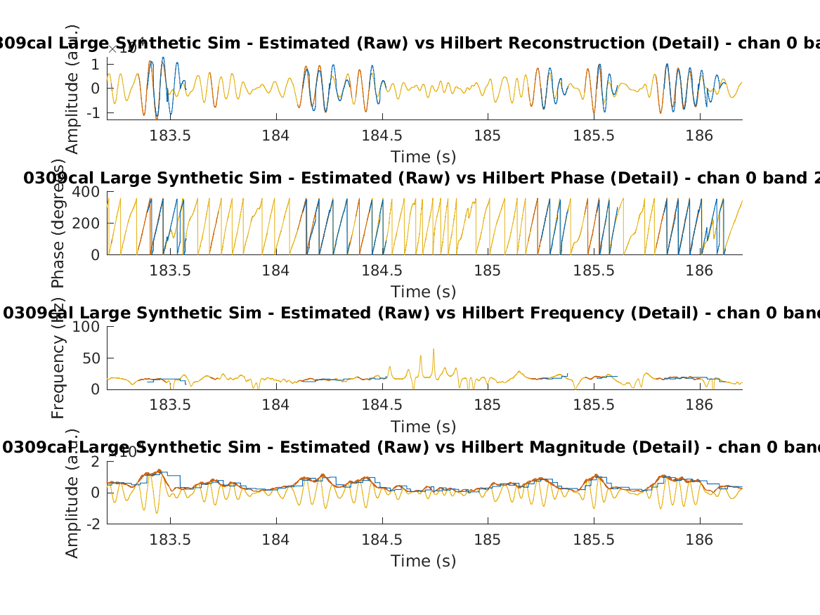
Figure 13: Estimated vs true analytic magnitude, phase, frequency, and waveform (real component). Estimated was performed using peak, trough, and zero-crossing analysis of the band-pass filter output. The estimated signal is shown in blue, during times when the oscillation detector indicated an oscillation was present. The analytic signal is shown in yellow, with orange regions indicating times when the instantaneous magnitude was at least twice the average magnitude. Instantaneous frequency of the analytic signal was computed as the smoothed derivative of phase. “Synthetic” dataset, IIR filters, beta band.

Comparing estimated magnitude and phase to those of the analytic signal computed from the band-pass-filtered signal shows whether the oscillation detector’s approximation of the instantaneous magnitude and phase are accurate. Figure 14 shows histograms and box plots of magnitude error normalized to the analytic signal magnitude (relative error) and of phase error with respect to the analytic signal phase. Representative rose plots of phase estimation error are shown for the alpha band (left) and medium gamma band (right). This analysis was performed using the “synthetic” dataset and IIR filters.

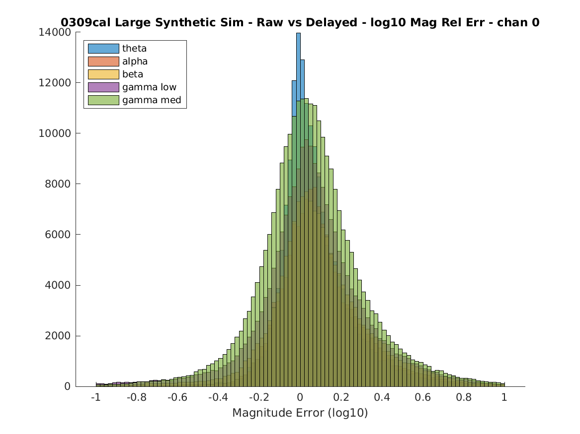
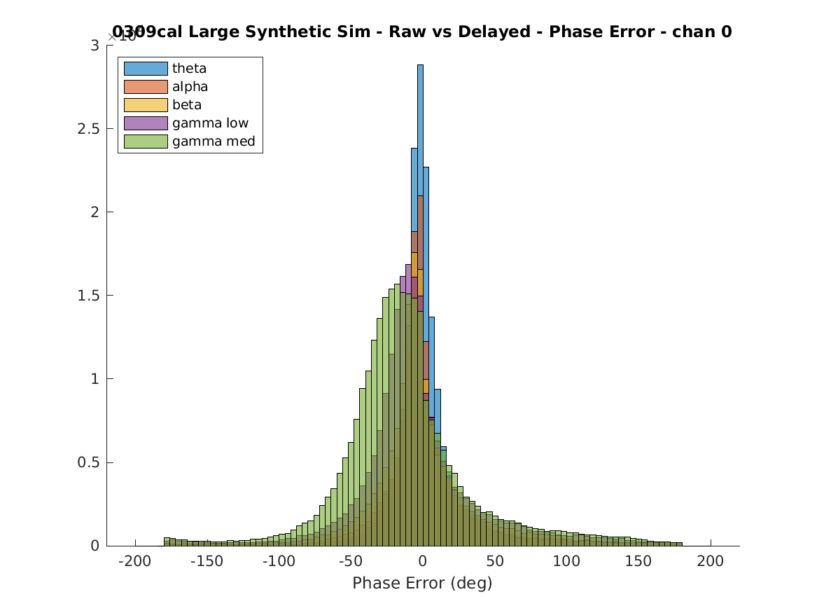
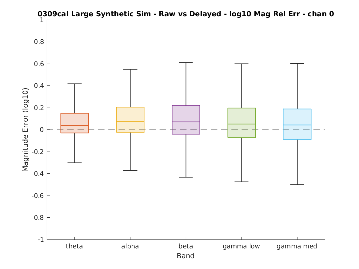
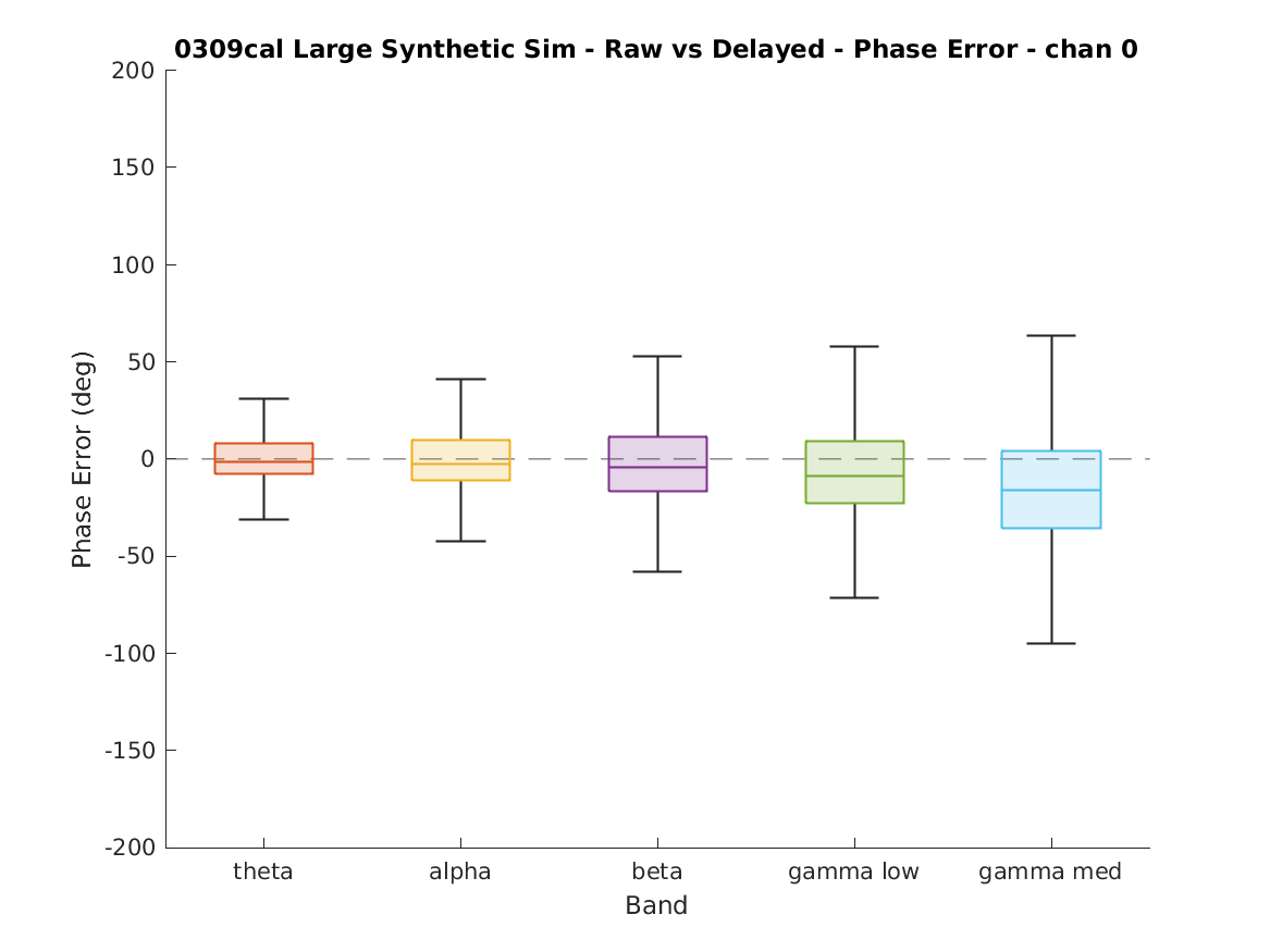
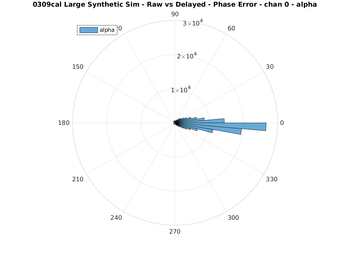
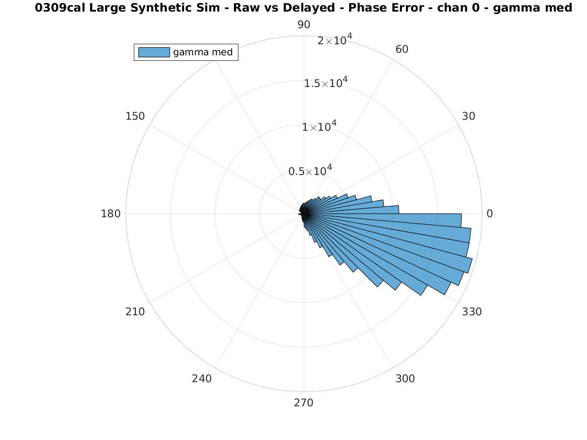
Figure 14: Normalized estimated magnitude error (left) and absolute estimated phase error (right) with respect to analytic signal magnitude and phase for the band-pass-filtered signal. The top row shows histograms of sample-by-sample error during oscillations. The middle row shows box plots of sample-by-sample error. The bottom row shows representative rose plots of phase error for the alpha band (left) and middle gamma band (right). IIR filters, “synthetic” dataset.

Magnitude error distributions are broad in all cases. This is because the envelopes of oscillations change on a timescale that is not substantially longer than the analysis timescale (one half-period of the oscillation). As the magnitude estimate is out of date by half a period, there may be a considerable difference between the estimated and actual magnitudes. This can be seen in the bottom strip in Figure 13; the estimated envelope is time-shifted relative to the actual envelope.

Phase error with respect to the band-pass-filtered wave is tightly clustered for theta, alpha, and beta bands ($\leq 20^{\circ}$ FWHM, $\leq 5^{\circ}$ offset). This error range is primarily due to frequency shifts during the oscillation. For higher-frequency bands (low and middle gamma), additional noise is present due to quantization of the detected half-period into an integer number of samples and due to noise perturbing the detected locations of zero-crossings (a single-sample shift at 100 Hz introduces a much larger phase error than a single-sample shift at 10 Hz).

Figure 15 shows histograms and box plots of magnitude error normalized to the analytic signal magnitude and of phase error with respect to the analytic signal phase for the “biological” dataset, using the same IIR filters. Representative rose plots of phase estimation error are again shown for the alpha band (left) and medium gamma band (right).

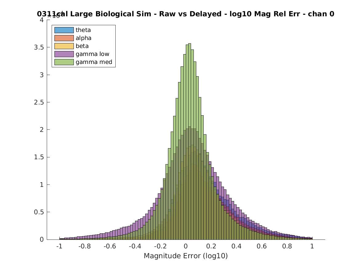
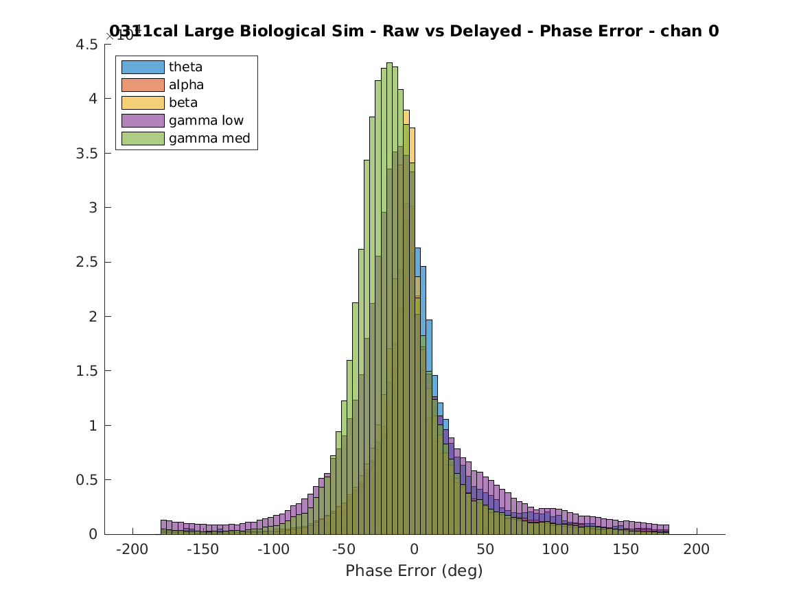
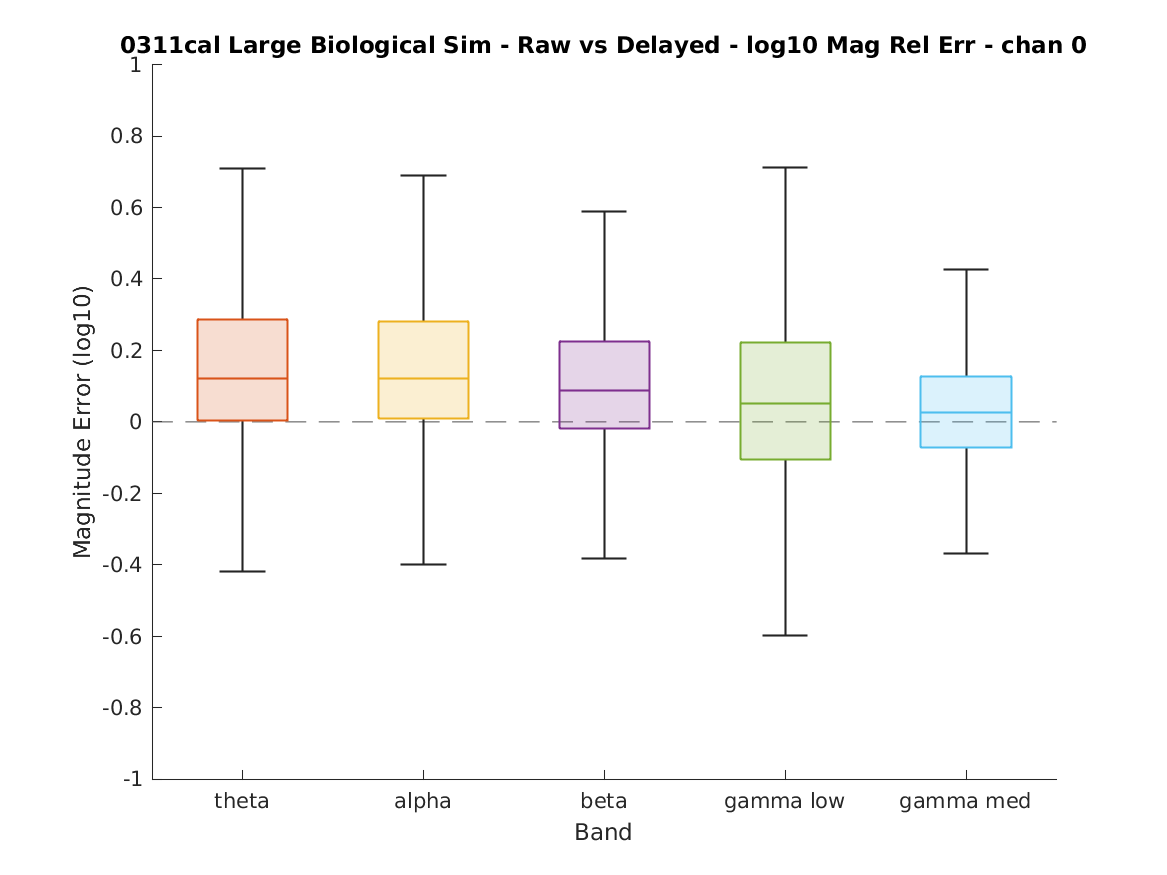
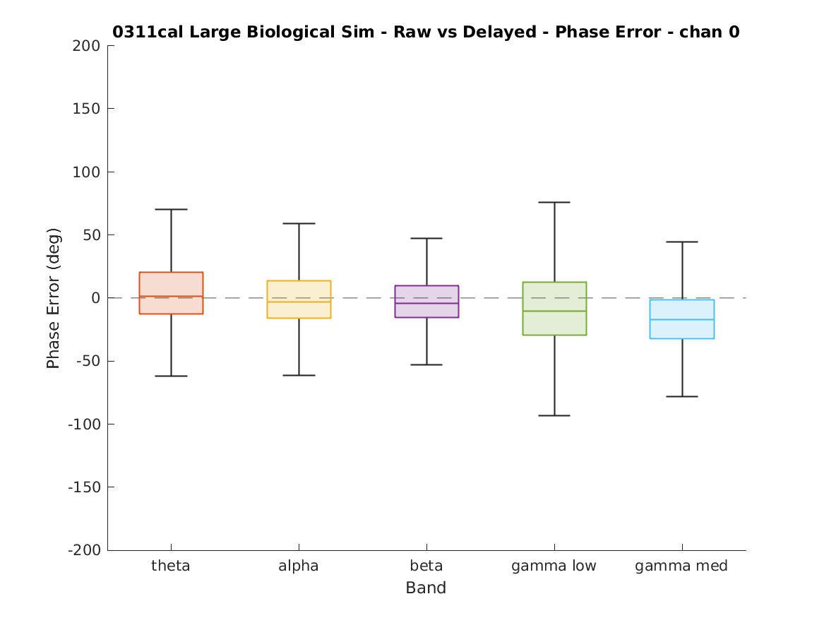
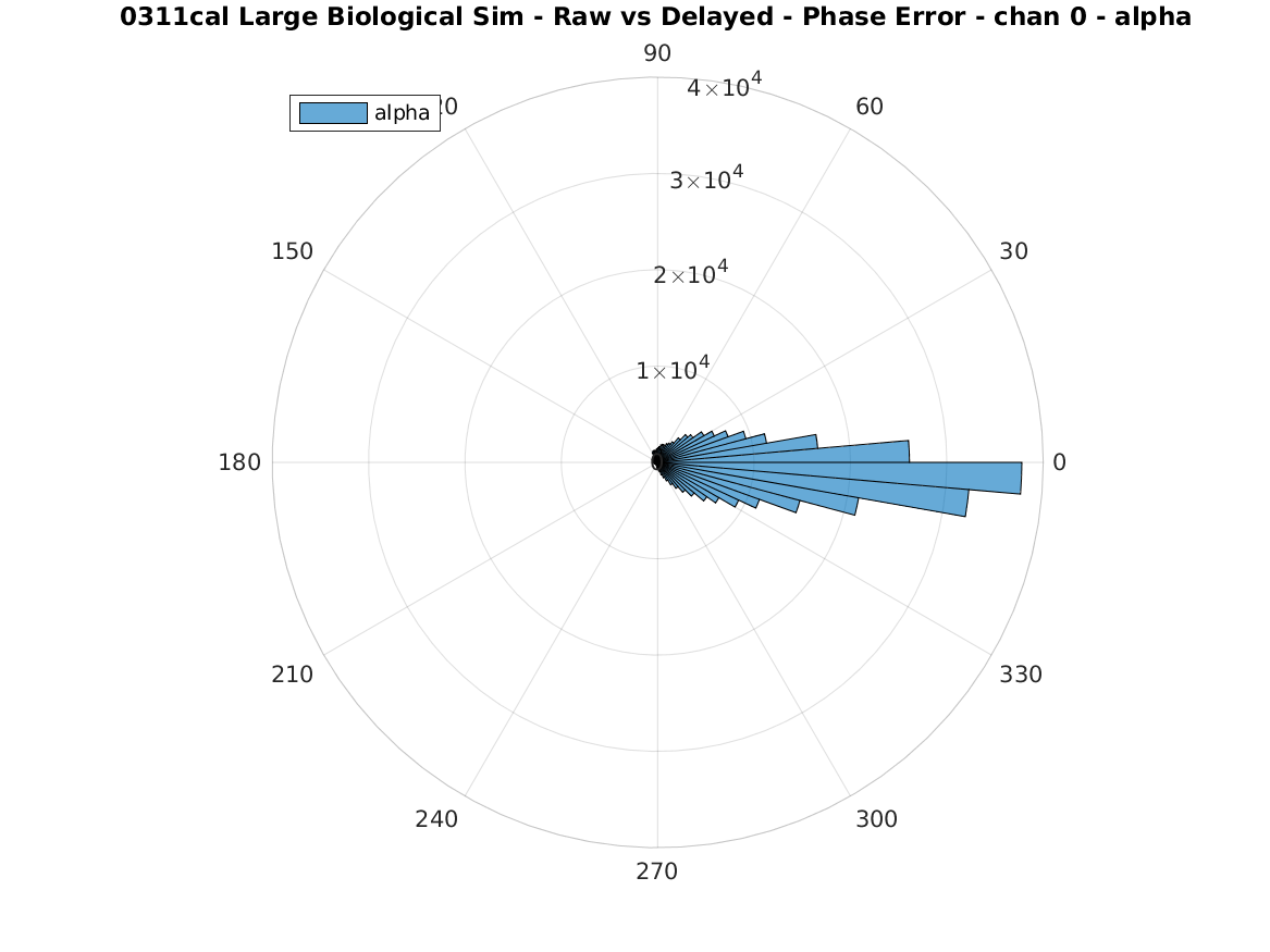
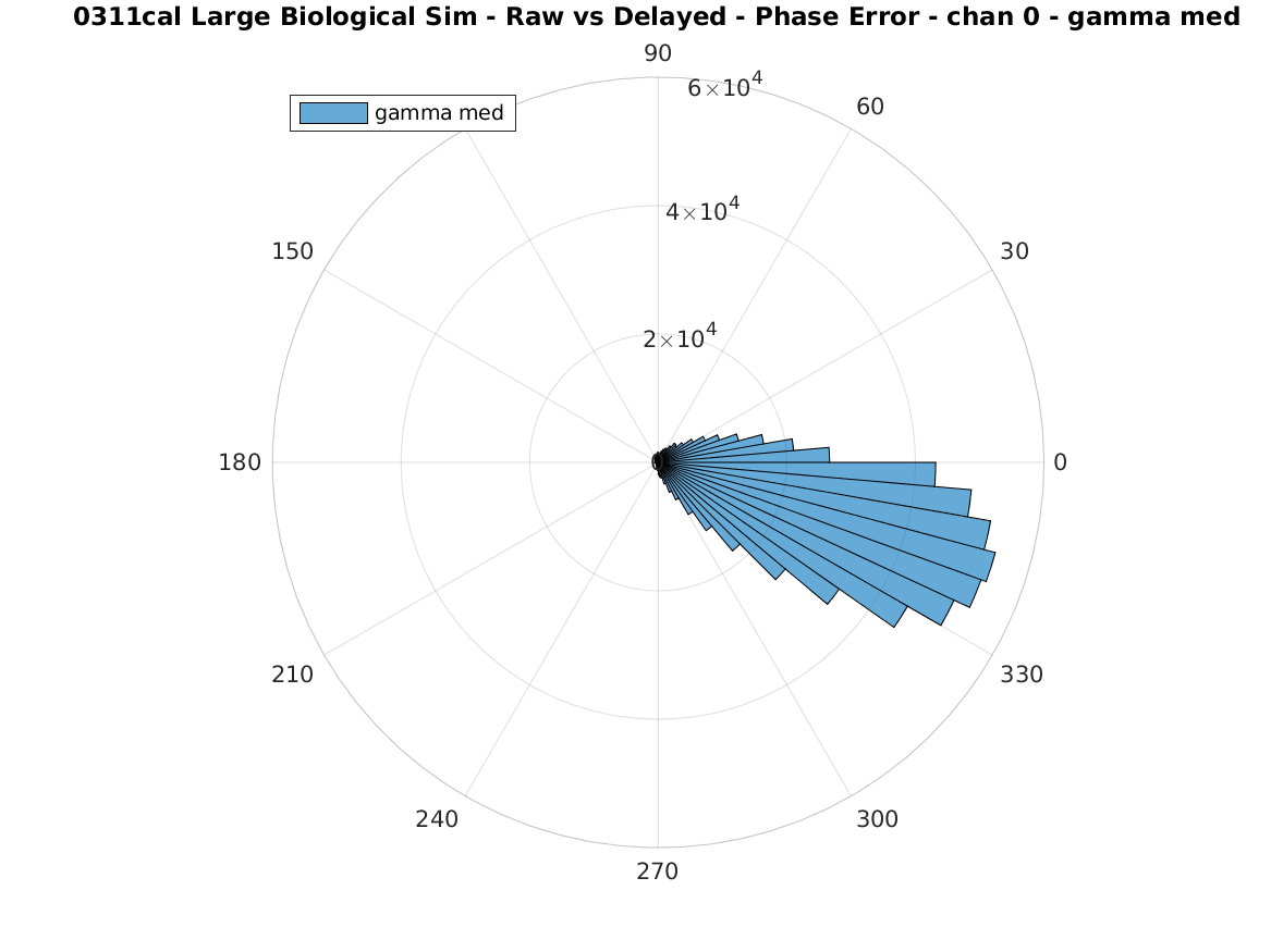
Figure 15: Normalized estimated magnitude error (left) and absolute estimated phase error (right) with respect to analytic signal magnitude and phase for the band-pass-filtered signal. The top row shows histograms of sample-by-sample error during oscillations. The middle row shows box plots of sample-by-sample error. The bottom row shows representative rose plots of phase error for the alpha band (left) and middle gamma band (right). IIR filters, “biological” dataset.

Magnitude error distributions are again broad (typically $\pm 40\%$ variation). Phase error with respect to the band-pass-filtered wave is less tightly clustered than with the “synthetic” dataset ($\leq 30^{\circ}$ FWHM, $\leq 5^{\circ}$ offset), but still well within the design requirements from Section II-A ($\leq 60^{\circ}$ FWHM). There is again additional spread in the middle gamma band.

IV-E Delay-Aligned and Phase-Aligned Triggering

Stimulation trigger alignment was characterized by specifying a desired delay in milliseconds from the rising or falling zero-crossing, or a desired phase angle, and measuring the distribution of delays and phase angles at which stimulation trigger signals were actually generated. This was evaluated with respect to two reference delays and phase angles: The “estimated” set (the output of the peak-and-trough estimator discussed in Section IV-D), and the “band-pass” set (the zero-crossings and instantaneous phase of the band-pass-filtered signal). Testing against the “estimated” set characterizes errors introduced by the trigger generation logic, while testing against the “band-pass” set characterizes the errors introduced by the combined processing pipeline (in particular, phase perturbation caused by mis-estimation of instantaneous frequency).

Figure 16 shows representative plots of trigger delay (top) and of delay error (bottom) for triggers scheduled with respect to the rising zero-crossing. The left set of plots shows trigger delay with respect to the estimated zero-crossings, and the right set of plots shows trigger delay with respect to the band-pass-filtered signal’s zero crossings. These measurements were taken using the beta band IIR filter and the “synthetic” dataset, and are plotted for multiple target delays. Figure 17 shows plots of delay error for the same tests case aggregated by band.

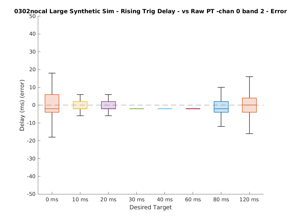
Figure 16: Representative plots of trigger delay (top) and delay error (bottom) for triggers scheduled with respect to the rising zero-crossing. Left: measurements with respect to the estimated signal. Right: measurements with respect to the band-pass-filtered signal. Measurements are grouped by desired delay. “Synthetic” dataset, beta band, IIR filters.

Figure 17: Plots of trigger delay error for triggers scheduled with respect to the rising zero-crossing, aggregated across all target delays. Left: measurements with respect to the estimated signal. Right: measurements with respect to the band-pass-filtered signal. Measurements are grouped by band. “Synthetic” dataset, IIR filters.

From Figure 17, delay-scheduled triggers are sent with minimal delay ($\pm 1$ sample at 500 sps) with respect to their intended trigger times. For many cases, the delay is negligible; as illustrated in Figure 16, error is dominated by either requested delays that are one or more periods long (beta band and higher-frequency) or by a requested delay of zero (beta band and lower-frequency). In the case of a delay of one period or longer, significant frequency drift is expected to occur in the input signal. In the case of a delay of zero, the trigger logic reschedules it for the following period, resulting in a delay of one period. Figure 18 shows plots of trigger phase error for each band (top and middle rows) and for the alpha band (bottom row) for triggers scheduled for specific phases. The left set of plots shows trigger phase with respect to the estimated signal phase, and the right set of plots shows trigger delay with respect to the phase of the analytic signal computed from the band-pass-filtered signal. As each oscillatory burst only resulted in one triggering event per target phase, the number of phase error samples was not sufficient to generate statistically meaningful plots of phase error for specific target phases.

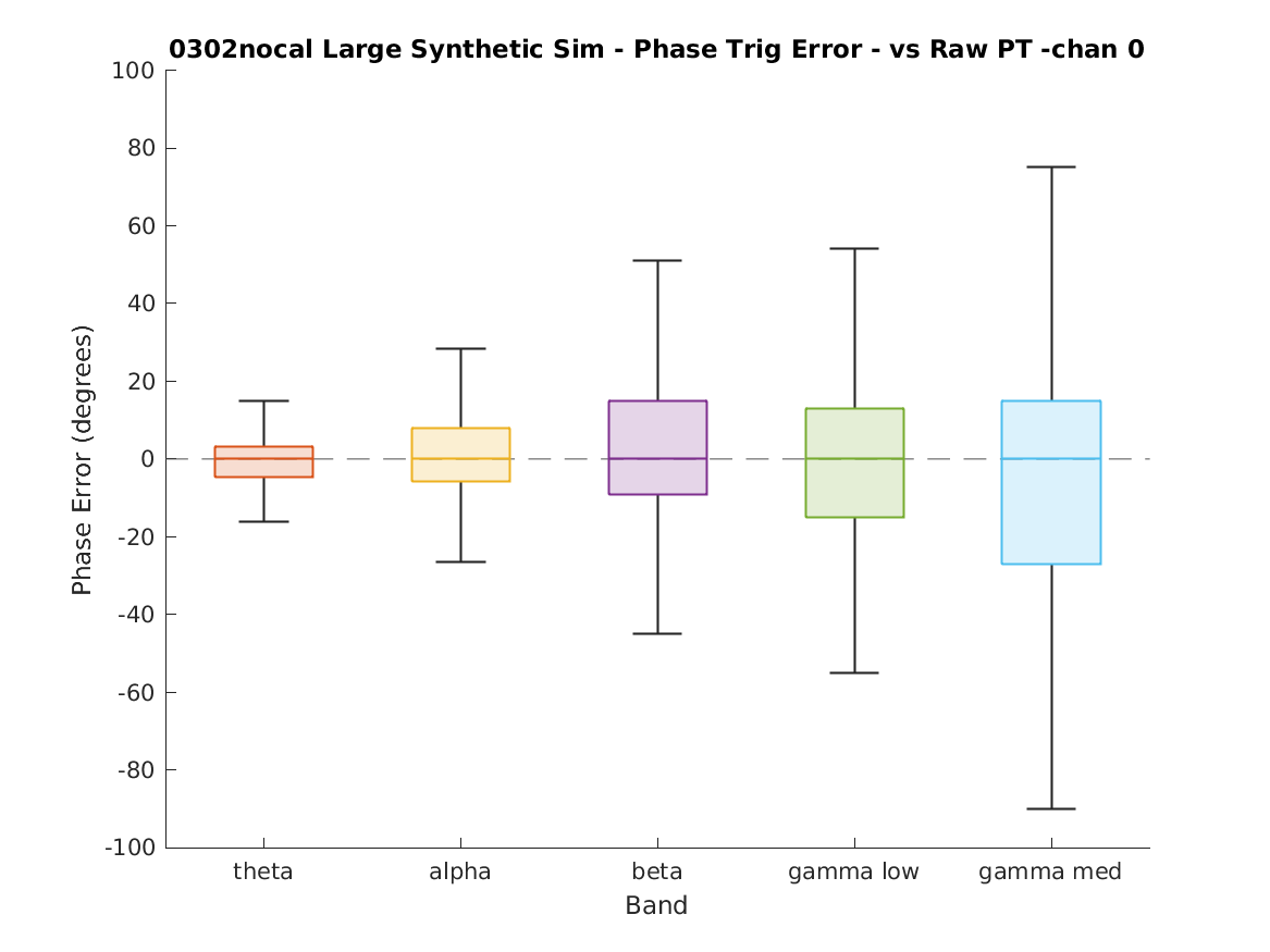
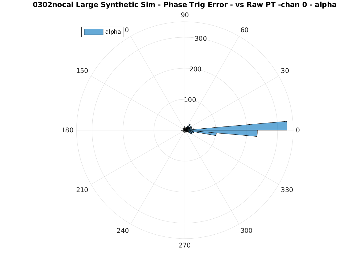
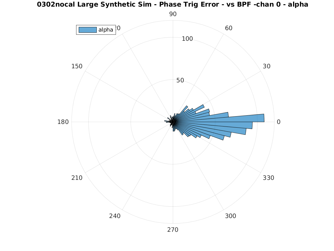
Figure 18: Plots of trigger phase error for triggers scheduled by phase, aggregated across all target phases. Left: measurements with respect to the estimated signal. Right: measurements with respect to the band-pass-filtered signal. Measurements are grouped by band. Bottom row: representative rose plots of phase error (alpha band). “Synthetic” dataset, IIR filters.

From Figure 18, the distribution of phase-scheduled trigger error with respect to the estimated signal has a narrow peak over a broad “noise floor”. This produces unusual statistics: the full-width half-maximum is one phase bin ($2^{\circ}$), but the inter-quartile range varies from $10^{\circ}$ to $30^{\circ}$. A larger sample size would be needed to identify the distribution (and hence source) of the noise floor in this plot. The distribution of phase-scheduled trigger error with respect to the band-pass-filtered signal shows a broader peak which again has a substantial “noise floor”: the full-width half-maximum varies from $20^{\circ}$ to $40^{\circ}$, with an inter-quartile range of approximately $50^{\circ}$. These values are broadly consistent with the expectation that the dominant source of trigger phase error is the phase estimation error described in Section IV-D (approx. $20^{\circ}$ FWHM), and continue to meet the design requirement of $\leq 60^{\circ}$ FWHM from Section II-A.

IV-F Delay Compensation for Infinite Impulse Response Filters

All causal filters introduce delay into the filtered signal. For FIR filters, this delay is constant, and for IIR filters, different frequency components are delayed by different amounts. To allow later processing stages to compensate for this, a calibration table of phase delay vs period was built. Figure 19 shows an example of the lookup table delay (step-wise curve), actual delay (red curve), and delay error after calibration (blue curve) for beta-band output after processing by the anti-aliasing IIR filter followed by the beta-band band-pass IIR filter (from Figure 12). A calibration table for a FIR filter would have only a single entry.

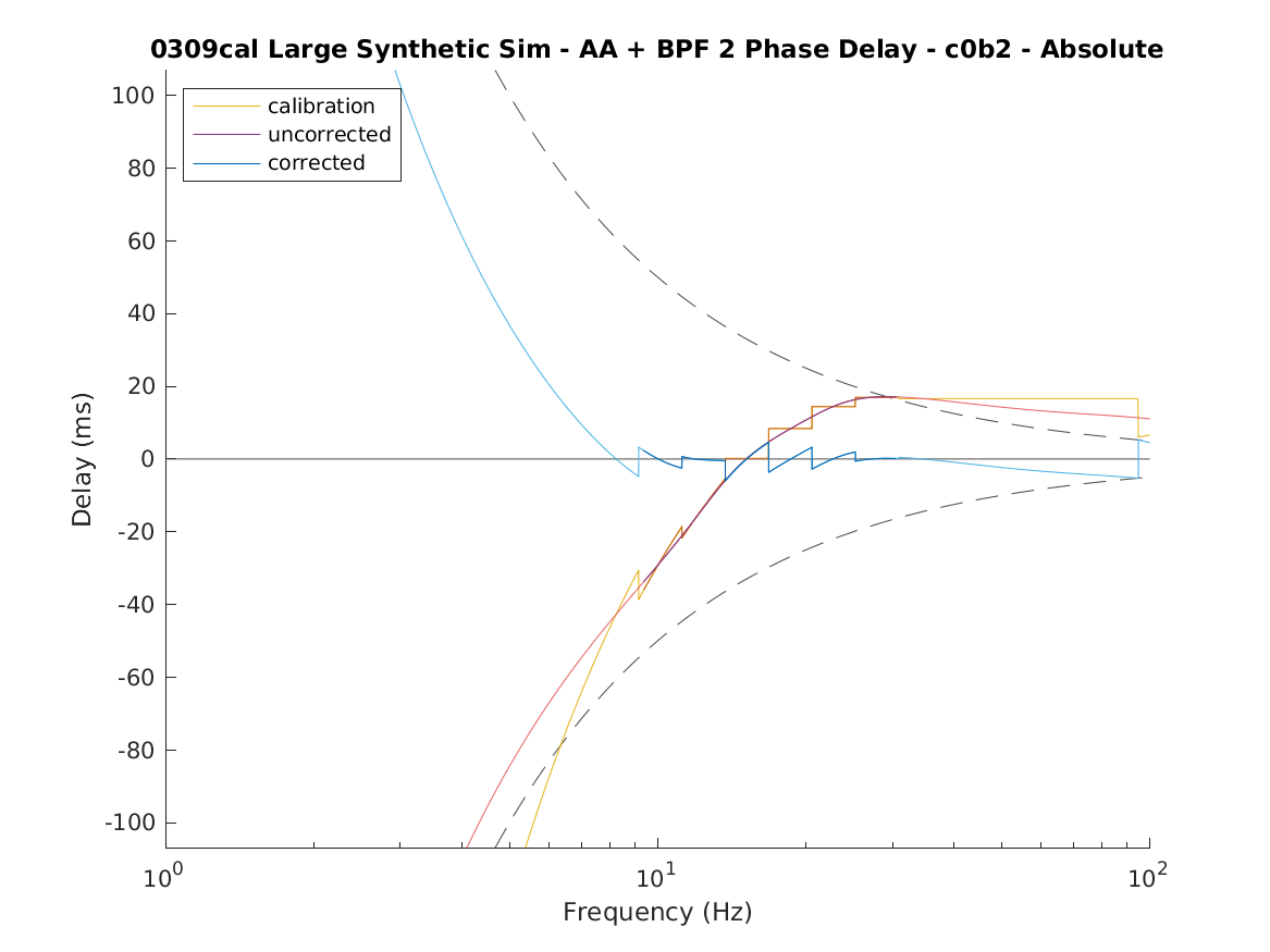
Figure 19: Phase delay calibration for the anti-aliasing IIR filter followed by the beta band IIR filter. The real phase delay (red curve) is approximated by a lookup table of calibration delays (step-wise curve). The resulting expected delay error after calibration is shown by the blue curve.

An ideal “zero-shift” version of the band-pass-filtered signal was created for each band. This signal was computed by using the gain component $G(\omega)$ of the filter’s transfer function (from Equation 2) as a non-causal filter to transform the wideband signal into a band-pass signal with zero time-shift (Equation 5). As the phase shift of this filter is zero at all frequencies, the phase delay and group delay of the filter are also zero. Time shift from the hardware anti-aliasing filter, software anti-aliasing filter, and software band-pass filters can be compensated in this manner.

$$\begin{split}Y_{0}(\omega)&=X(\omega)\cdot G(\omega)\\ y_{0}(t)&=\mathcal{F}^{-1}\left\{G(\omega)\cdot\mathcal{F}\{x(t)\}\right\}\end{split}$$ (5)

Estimated magnitude and phase after delay calibration were compared to those of the “zero-shift” band-pass-filtered signal using the same approach as in Section IV-D. Figure 20 shows histograms and box plots of raw estimates (left) and calibrated estimates (right) of magnitude and phase with respect to the “zero-shift” signal. Magnitude error (top row) was normalized with respect to analytic signal magnitude (relative error), and phase error (middle row) was taken as the difference between estimated phase and the analytic signal phase. The bottom row shows a representative rose plot of phase estimates (beta band). This analysis was performed using the “synthetic” dataset and IIR filters.

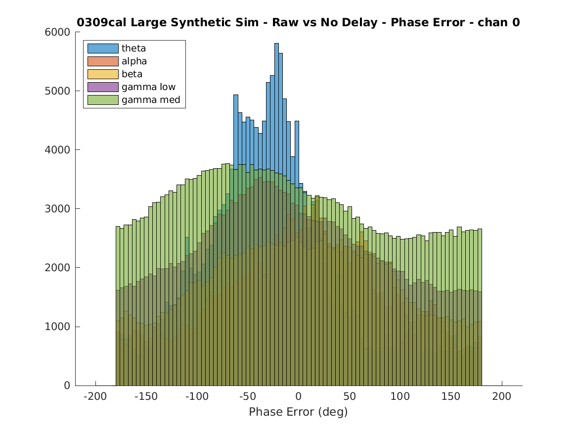
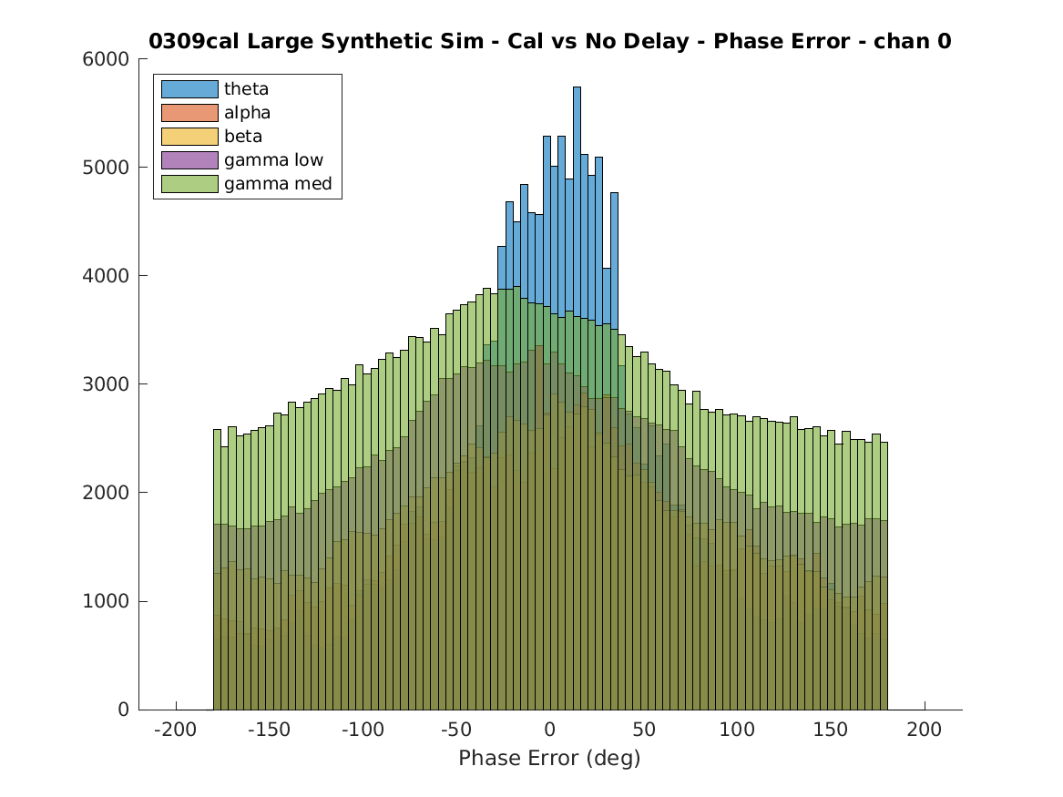
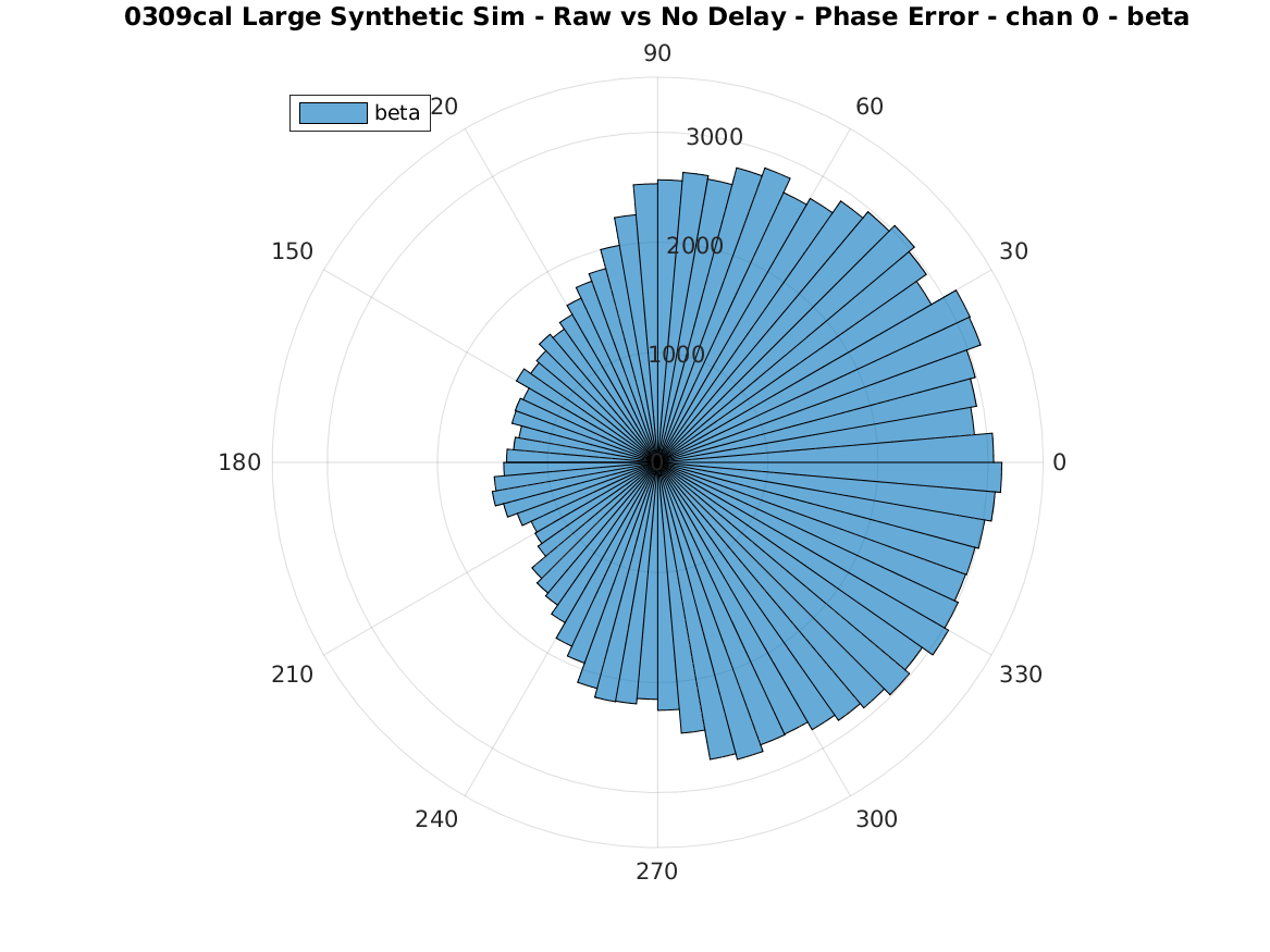
Figure 20: Normalized estimated magnitude error (top), absolute estimated phase error (middle), and beta band estimated phase error (bottom) for raw estimated magnitude and phase (left) and calibrated estimated magnitude and phase (right). Error was measured with respect to the “zero time shift” band-pass-filtered signal. IIR filters, “synthetic” dataset.

The magnitude estimate is not affected by calibration, so the magnitude estimation error is unchanged between the “raw” and “calibrated” columns in Figure 20. The magnitude error distribution is much broader when measured with respect to the “zero-shift” signal that when measured with respect to the delayed band-pass-filtered signal. This can be understood as a consequence of the observation that the signal envelope varies on a timescale comparable to the oscillation period: with the filter’s time delay exposed, magnitude has more time to change. This results in somewhat larger variation (approx. $\pm 60\%$).

The phase error distribution measured with respect to the “zero-shift” signal shows three significant properties. First, aside from the distribution in the theta band, none of the error distributions shows a sharp peak; instead the distribution has a broad hill over a high uniform background. This makes it difficult to meaningfully extract peak width statistics. Second, the location of the broad peak does shift with calibration, having significant bias before calibration and being zero-averaged afterwards. Third, the shape of the rose plot changes substantially during calibration, narrowing for the beta band and lower frequencies. The primary conclusion to be drawn is that there is a large additional source of phase estimation noise introduced by the IIR band-pass filters that is not adequately compensated by delay calibration. This problem is worse in the “biological” dataset.

There are several potential sources for phase estimation error. These can broadly be classified into sources that involve rapid perturbation of phase or frequency (due to non-stationary frequency or due to noise), sources that cause the oscillating signal to cease to be a pure tone (such as harmonic overtones or other strong out-of-band tones), and sources that involve neither of these but that cause the frequency of the oscillation to be mis-estimated, resulting in an incorrect delay calibration lookup value. Sources of this last type can readily be investigated and might be corrected.

Mis-detection of oscillation frequency can be evaluated by plotting a histogram of estimated vs. actual instantaneous frequency. Representative plots showing heat-maps of estimated frequency vs analytic signal frequency in the beta band are shown in Figure LABEL:fig-validation-cal-iirfreqfreq. The frequency band is indicated by the white lines. One histogram bin width represents an approximately 5% change in frequency. These plots confirm that for both “biological” and “synthetic” datasets a large number of samples have mis-estimated frequency, which will lead to incorrect delay compensation.

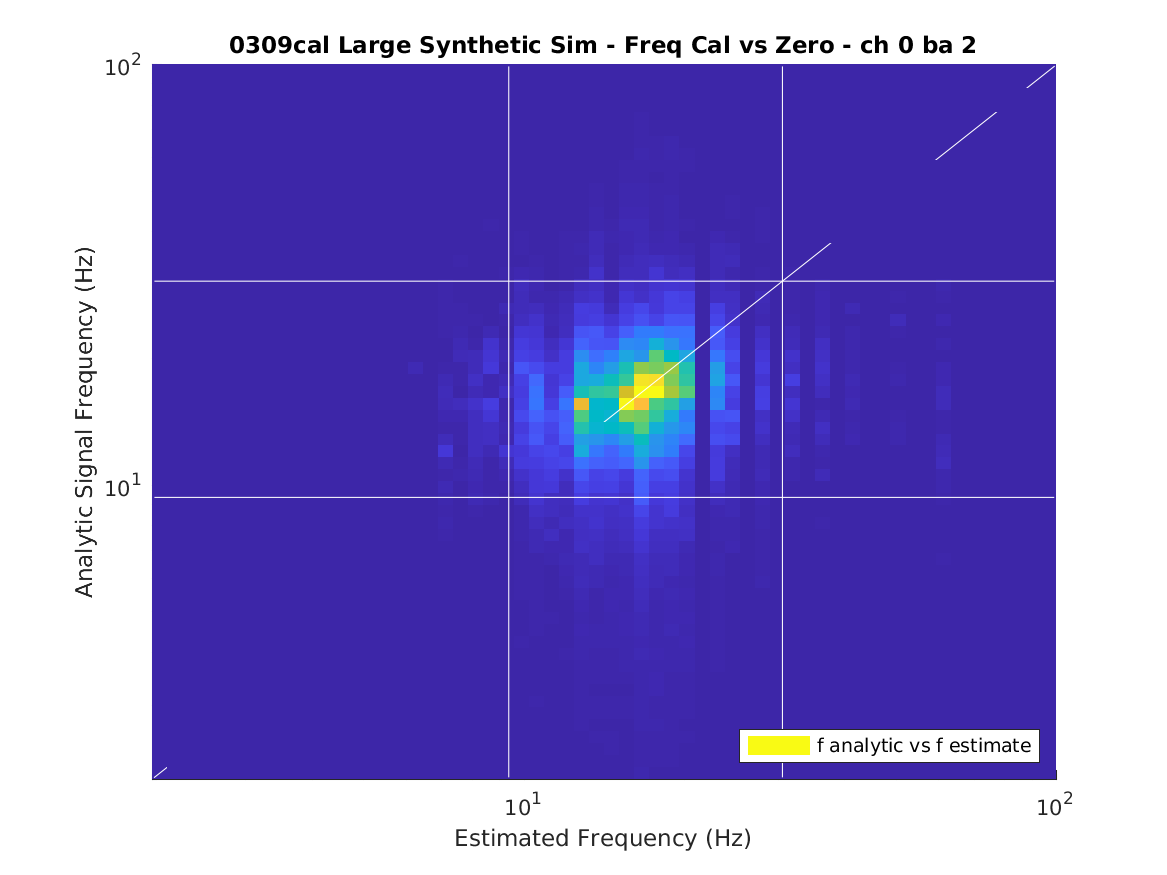
Figure 21: Heat map of estimated frequency vs analytic signal instantaneous frequency, using the “synthetic” dataset (left) and the “biological” dataset (right). The top row shows the raw frequency estimate and the delayed band-pass-filtered signal’s instantaneous frequency, and the bottom row shows the calibrated frequency estimate and the “zero time shift” band-pass-filtered signal’s instantaneous frequency. One bin width represents an approximately 5% change in frequency. IIR filters, beta band.

The effects of poorly-estimated frequency can be evaluated by plotting a two-dimensional histogram of calibration delay applied vs the analytic signal frequency for each sample during oscillation events. For clarity, this may instead be plotted as the residue after the calibration delay is subtracted from the known phase delay at that instantaneous frequency; the resulting plot will be a phase delay error plot, with a desired value of zero. A representative plot showing a heat-map of phase delay compensation error is shown in Figure 22 (beta band IIR filter, “synthetic” dataset). The saw-tooth curve in the plot represents the calibration lookup table bin size. This is narrower than the frequency smearing distance in the plot, indicating that bin quantization is not a significant source of error. Frequency smearing covers a substantial fraction of the frequency band, causing phase delay compensation errors that are large compared to the scale of the residue expected after phase delay compensation.

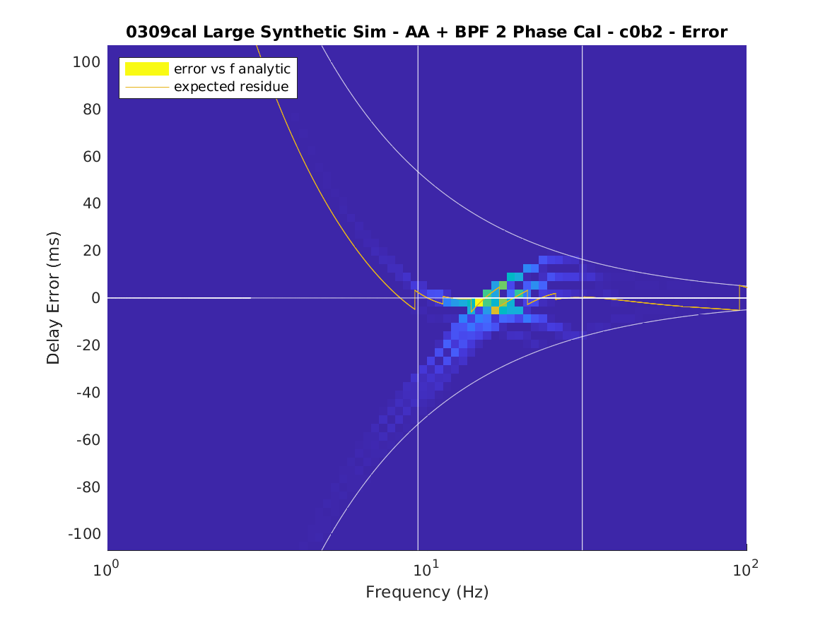
Figure 22: Phase delay residue after compensating for the anti-aliasing filter and the beta band IIR filter. The yellow curve is the expected estimation error, the white vertical bars indicate the pass-band edges, the white curves show the delay corresponding to $\pm$ half a period, and the heat map shows the distribution of phase delay residue versus the analytic signal’s instantaneous frequency. Beta band IIR filter, “synthetic” dataset.

One source of potentially incorrect frequency estimates is a bad estimate of oscillation frequency during the first half-period of the oscillation. As described in Section III, the frequency estimate is delayed by up to half an oscillation period. When an oscillation is first detected, the frequency estimate is from a time interval prior to the oscillation’s magnitude excursion, when the signal-to-noise ratio may have been poor. This can be evaluated by plotting a two-dimensional histogram of estimated frequency error over time. Representative plots showing heat-maps of normalized estimated frequency (relative error) for the alpha band are shown in Figure 23. While there is a substantial amount of mis-detection at all times, the alpha band and other low-frequency bands do have more error during the first half-period of the oscillation in both the “synthetic” and “biological” traces.

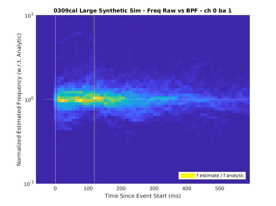
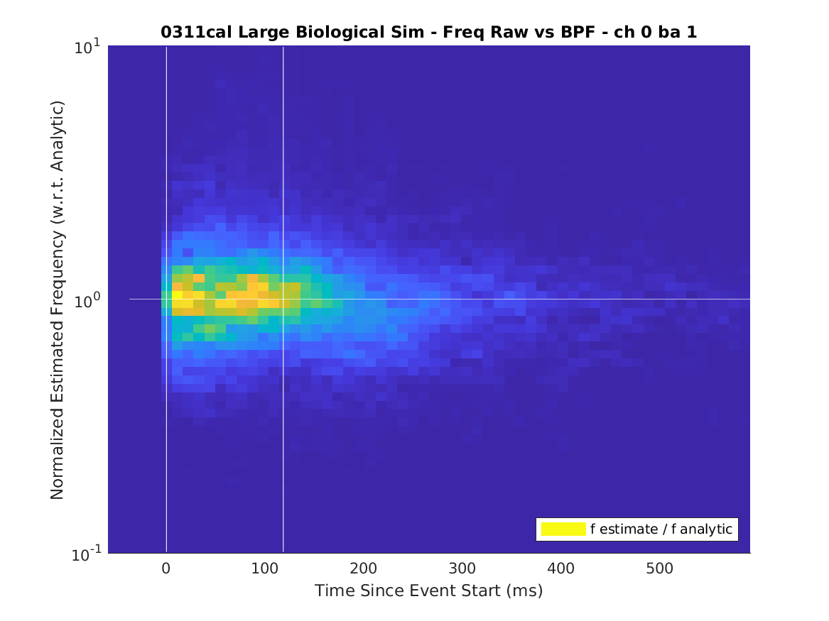
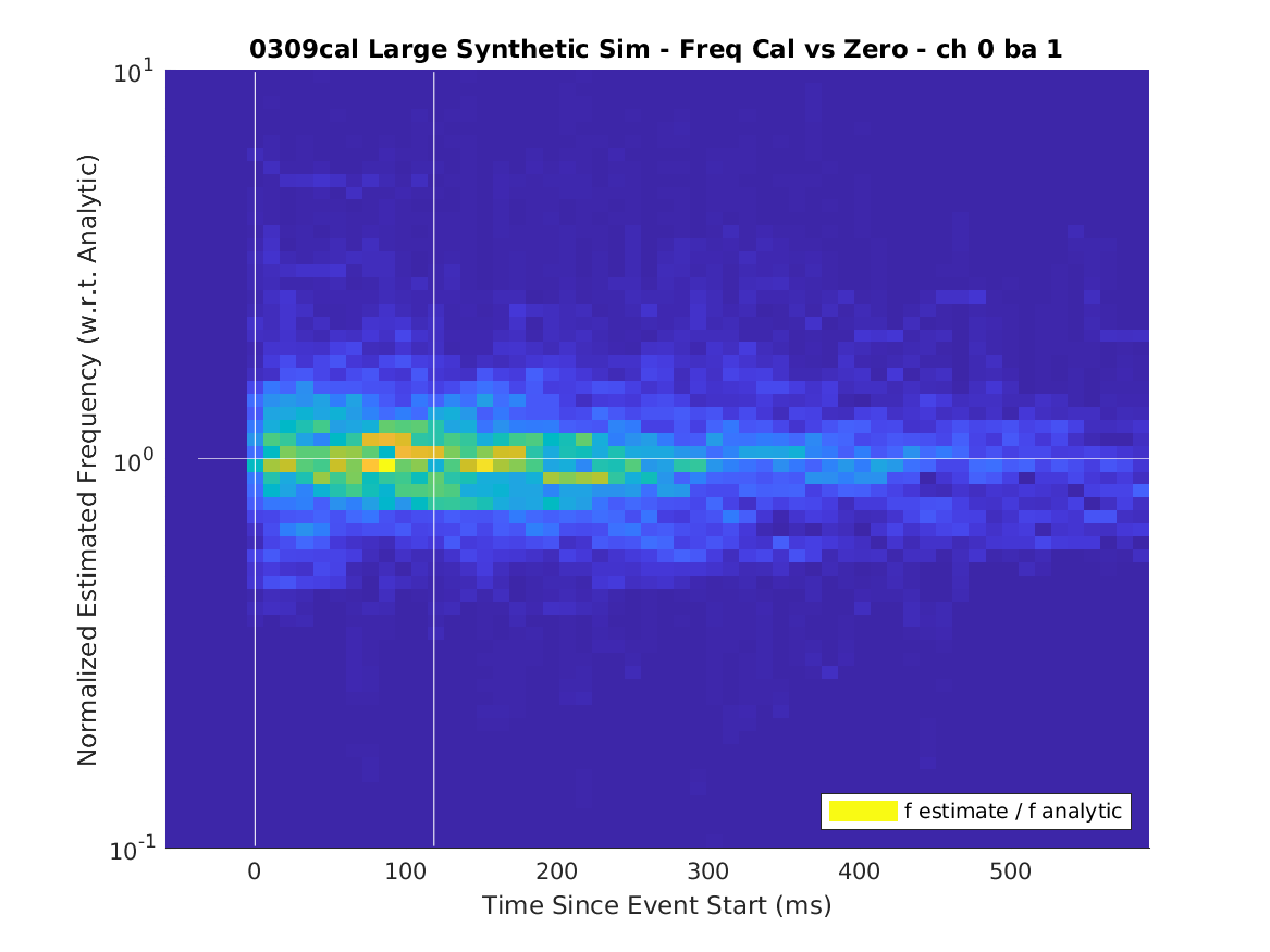
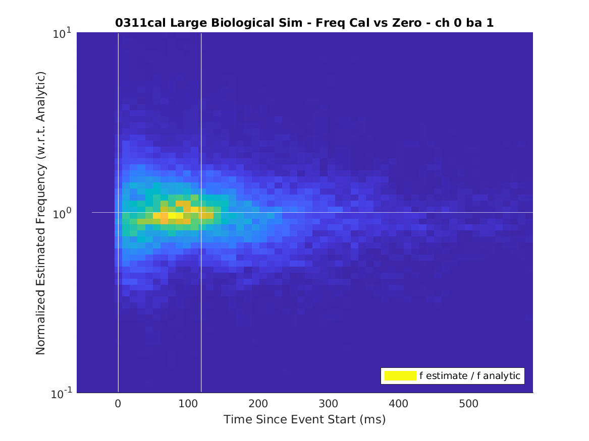
Figure 23: Heat map of estimated frequency error over time, using the “synthetic” dataset (left) and the “biological” dataset (right). The top row shows the raw frequency estimate normalized to the delayed band-pass-filtered signal’s instantaneous frequency, and the bottom row shows the calibrated frequency estimate normalized to the “zero time shift” band-pass-filtered signal’s instantaneous frequency. IIR filters, alpha band.

V Conclusion

A modular, scalable signal processing framework has been presented that is capable of detecting and characterizing oscillations on the local field potential of neural signals, and of generating trigger signals to allow phase-aligned and delay-aligned stimulation to be performed. As a case study, this framework was used to prototype an “off-line” workstation-based stimulation controller and an “on-line” microcontroller-based stimulation controller.

The workstation-based “off-line” implementation was used to validate the performance of the oscillation detection and stimulation control architecture. Phase could be estimated within $\frac{3}{4}$ period of oscillation onset, with an error distribution FWHM of $20^{\circ}$ for synthetic data and $30^{\circ}$ for biological data, with respect to the instantaneous frequency of the band-pass-filtered signal.

Stimulation pulses with timing specified relative to zero-crossings in the signal waveform could be generated with an error distribution FWHM of 2 ms with respect to the band-pass-filtered signal. Stimulation pulses timed to specific phases in the signal waveform could be generated with an error distribution FWHM of $40^{\circ}$ with respect to the band-pass-filtered signal. This meets the minimum requirements for closed-loop experiments studying phase-aligned stimulation.

The microcontroller-based “on-line” implementation was used to demonstrate that a usable oscillation detector and stimulation controller could be built with severely constrained hardware resources, making the case for application of this framework to systems with thousands of channels and/or hundreds of bands on readily-available hardware. A microcontroller-based implementation was presented that duplicated the functionality of the ‘off-line” implementation in real-time with a single channel, a single band, and using infinite impulse response filters. This was done with an estimated processing budget of 100 kMAC/sec, compared to an estimated processing budget of at least 3 MMAC/sec$\cdot$channel provided by readily available user-configurable electrophysiology equipment.

In conclusion, the signal processing framework presented was shown to be sufficient for rapid prototyping of controllers for phase-aligned neural stimulation and is readily adapted to large-scale implementations using FPGA-based or DSP-based electrophysiology controllers.

Christopher Thomas Christopher Thomas is a research scientist with the Attention Circuits Control Laboratory in the Department of Psychology at Vanderbilt University, where he specializes in signal processing and embedded systems. He received his PhD from York University in Toronto, Canada for his work on image sensors.

Thilo Womelsdorf Thilo Womelsdorf is Associate Professor in the Departments of Psychology and Biomedical Engineering at Vanderbilt University, where he leads the Attention Circuits Control Laboratory. His research investigates how neural circuits learn and control attentional allocation in non-human primates and humans. Before arriving at Vanderbilt he led a systems neuroscience lab in Toronto (York University), receiving in 2017 the prestigious E.W.R. Steacie Memorial Fellowship for his work bridging the cell- and network- levels of understanding how brain activity dynamics relate to behavior.

References

- [1] G. Buzsaki, N. Logothetis, and W. Singer, “Scaling brain size, keeping timing: Evolutionary preservation of brain rhythms,” Neuron, vol. 80, no. 3, pp. 751–764, 2013.
- [2] G. Buzsaki, “Large-scale recording of neuronal ensembles,” Nature Neuroscience, vol. 7, pp. 446–451, 2004.
- [3] T. Womelsdorf, B. Lima, M. Vinck, R. Oostenveld, W. Singer, S. Neuenschwander, and P. Fries, “Orientation selectivity and noise correlation in awake monkey area v1 are modulated by the gamma cycle,” Proceedings of the National Academy of Sciences, vol. 109, no. 11, pp. 4302–4307, 2012.
- [4] C. Kayser, M. A. Montemurro, N. K. Logothetis, and S. Panzeri, “Spike-phase coding boosts and stabilized information carried by spatial and temporal spike patterns,” Neuron, vol. 61, no. 4, pp. 597–608, 2009.
- [5] B. Voloh, M. Oemisch, and T. Womelsdorf, “Phase of firing coding of learning variables across prefrontal cortex, anterior cingulate cortex and striatum during feature learning,” Nature Communications, vol. 11, no. 4669, 2020.
- [6] H. K. Turesson, N. K. Logothetis, and K. L. Hoffman, “Category-selective phase coding in the superior temporal sulcus,” Proceedings of the National Academy of Sciences, vol. 109, no. 47, pp. 19 438–19 443, 2012.
- [7] M. Lundqvist, P. Herman, M. R. Warden, S. L. Brincat, and E. K. Miller, “Gamma and beta bursts during working memory readout suggest roles in its volitional control,” Nature Communications, vol. 9, no. 394, 2018.
- [8] F. van Ede, A. J. Quinn, M. W. Wollrich, and A. C. Nobre, “Neural oscillations: Sustained rhythms or transient burst-events?” Trends in Neurosciences, vol. 41, no. 7, pp. 415–417, 2018.
- [9] M. A. Sherman, S. Lee, R. Shaw, S. Haegens, C. A. Thorn, M. S. Hamalainen, C. I. Moore, and S. R. Jones, “Neural mechanisms of transient neocortical beta rhythms: Converging evidence from humans, computational modeling, monkeys, and mice,” Proceedings of the National Academy of Sciences, vol. 113, no. 33, pp. E4885–E4894, 2016.
- [10] B. Voloh, T. A. Valiante, S. Everling, and T. Womelsdorf, “Theta-gamma coordination between anterior cingulate and prefrontal cortex indexes correct attention shifts,” Proceedings of the National Academy of Sciences, vol. 112, no. 27, pp. 8457–8462, 2015.
- [11] J. Feingold, D. J. Gibson, B. DePasquale, and A. M. Graybiel, “Bursts of beta oscillation differentiate postperformance activity in the striatum and motor cortex of monkeys performing movement tasks,” Proceedings of the National Academy of Sciences, vol. 112, no. 44, pp. 12 687–13 692, 2015.
- [12] J. R. Huxter, T. J. Senior, K. Allen, and J. Csicsvari, “Theta phase-specific codes for two-dimensional position, trajectory and heading in the hippocampus,” Nature Neuroscience, vol. 11, no. 5, pp. 587–594, May 2008.
- [13] M. Siegel, M. R. Warden, and E. K. Miller, “Phase-dependent neuronal coding of objects in short-term memory,” Proceedings of the National Academy of Sciences, vol. 106, no. 50, pp. 21 341–21 346, 2009.
- [14] M. Vinck, T. Womelsdorf, and P. Fries, “Gamma-band synchronization and information transmission,” in Principles of Neural Coding, R. Q. Quiroga and S. Panzeri, Eds. CRC Press, 2013, ch. 23, pp. 449–469.
- [15] M. Vinck, B. Lima, T. Womelsdorf, R. Oostenveld, W. Singer, S. Neuenschwander, and P. Fries, “Gamma-phase shifting in awake monkey visual cortex,” Journal of Neuroscience, vol. 30, no. 4, pp. 1250–1257, 2010.
- [16] R. Polania, M. A. Nitsche, and C. C. Ruff, “Studying and modifying brain function with non-invasive brain stimulation,” Nature Neuroscience, vol. 21, pp. 174–187, 2018.
- [17] M. A. Lebedev and M. A. L. Nicolelis, “Brain-machine interfaces: From basic science to neuroprostheses and neurorehabilitation,” Physiological Reviews, vol. 97, pp. 767–837, 2017.
- [18] S. Qiao, J. I. Sedillo, K. A. Brown, B. Ferrentino, and B. Pesaran, “A causal network analysis of neuromodulation in the mood processing network,” Neuron, vol. 107, pp. 1–14, 2020.
- [19] L. Grosenick, J. H. Marshel, and K. Deisseroth, “Closed-loop and activity-guided optogenetic control,” Neuron, vol. 86, no. 1, pp. 106–139, 2015.
- [20] S. Zanos, I. Rembado, D. Chen, and E. E. Fetz, “Phase-locked stimulation during cortical beta oscillations produces bidirectional synaptic plasticity in awake monkeys,” Current Biology, vol. 28, pp. 1–12, 2018.
- [21] J. H. Siegle and M. A. Wilson, “Enhancement of encoding and retrieval functions through theta phase-specific manipulation of hippocampus,” p. e03061, 2014.
- [22] H. Cagnan, D. Pedrosa, S. Little, A. Pogosyan, B. Cheeran, T. Aziz, A. Green, J. Fitzgerald, T. Foltynie, P. Limousin, L. Zrinzo, M. Hariz, K. J. Friston, T. Denison, and P. Brown, “Stimulating at the right time: phase-specific deep brain stimulation,” Brain, vol. 140, no. 1, pp. 132–145, 2017.
- [23] G. Weerasinghe, B. Duchet, H. Cagnan, P. Brown, C. Bick, and R. Bogacz, “Predicting the effects of deep brain stimulation using a reduced coupled oscillator model,” PLOS Computational Biology, vol. 15, no. 8, p. e1006575, 2019.
- [24] E. Blackwood, M. chen Lo, and A. S. Widge, “Continuous phase estimation for phase-locked neural stimulation using an autoregressive model for signal prediction,” in Proc. 40th Conf. IEEE Engineering in Medicine and Biology Society, 2018, pp. 4736–4739.
- [25] L. L. Chen, R. Madhaan, B. I. Rapoport, and W. S. Anderson, “Real-time brain oscillation detection and phase-locked stimulation using autoregressive spectral estimation and time-series forward prediction,” IEEE Transactions on Biomedical Engineering, vol. 60, no. 3, pp. 753–762, 2013.
- [26] G. Karvat, A. Schneider, M. Alyahyay, F. Steenbergen, M. Tangermann, and I. Diester, “Real-time detection of neural oscillation bursts allows behaviorally relevant neurofeedback,” Communications Biology, vol. 3, no. 72, pp. 1–10, 2020.
- [27] O. Talakoub, A. G. P. Schjetnan, T. A. Valiante, M. R. Popovic, and K. L. Hoffman, “Closed-loop interruption of hippocampal ripples through fornix stimulation in the non-human primate,” Brain Stimulation, vol. 9, pp. 911–918, 2016.
- [28] “RZ2 BioAmp Processor,” https://www.tdt.com/files/manuals/Sys3Manual/RZ2.pdf, accessed: 2020-08-26.
- [29] “Hardware Processing Platform (HPP): Getting Started Guide,” https://neuralynx.com/documents/HPP_Getting_Started_Guide.pdf, accessed: 2020-08-26.
- [30] M. Oemisch, S. Westendorff, M. Azimi, S. A. Hassani, S. Ardid, P. Tiesinga, and T. Womelsdorf, “Feature-specific prediction errors and surprise across macaque fronto-striatal circuits,” Nature Communications, vol. 10, no. 176, 2019.
- [31] B. P. Bean, “The action potential in mammalian central neurons,” Nature Reviews Neuroscience, vol. 8, pp. 451–465, 2007.
- [32] K. B. Boroujeni, P. Tiesinga, and T. Womelsdorf, “Adaptive spike-artifact removal from local field potentials uncovers prominent beta and gamma band neuronal synchronization,” Journal of Neuroscience Methods, p. 330:108485, 2020.
- [33] G. Buzsaki, C. A. Anastassiou, and C. Koch, “The origin of extracellular fields and currents – eeg, ecog, lfp and spikes,” Nature Reviews Neuroscience, vol. 13, pp. 407–420, May 2012.
- [34] K. J. Miller, L. B. Sorensen, J. G. Ojemann, and M. den Nijs, “Power-law scaling in the brain surface electric potential,” PLOS Computational Biology, vol. 5, no. 12, p. e1000609, 2009.
- [35] J. Milstein, F. Mormann, I. Fried, and C. Koch, “Neuronal shot noise and brownian 1/f2 behavior in the local field potential,” PLOS One, vol. 4, no. 2, p. e4338, 2009.
- [36] M. Steriade, “Corticothalamic resonance, states of vigilance and mentation,” Neuroscience, vol. 101, no. 2, pp. 243–276, 2000.
- [37] T. Womelsdorf, T. Valiante, N. T. Sahin, K. J. Miller, and P. Tiesinga, “Dynamic circuit motifs underlying rhythmic gain control, gating, and integration,” Nature Neuroscience, vol. 17, pp. 1031–1039, 2014.
- [38] G. Buzsaki, Rhythms of the Brain. Oxford University Press, 2006.
- [39] P. Y. Ktonas and N. Papp, “Instantaneous envelope and phase extraction from real signals: Theory, implementation, and an application to eeg analysis,” Signal Processing, vol. 2, no. 4, pp. 373–385, 1980.
- [40] S. Cole and B. Voytek, “Cycle-by-cycle analysis of neural oscillations,” Journal of Neurophysiology, vol. 122, no. 2, pp. 849–861, 2019.
- [41] J. C. Principe and A. J. Brockmeier, “Representing and decomposing neural potential signals,” Current Opinion in Neurobiology, vol. 31, pp. 13–17, 2015.
- [42] R. T. Canolty and T. Womelsdorf, “Multiscale adaptive gabor expansion (mage): Improved detection of transient oscillatory burst amplitude and phase,” 2019, https://www.biorxiv.org/content/10.1101/369116v4.abstract.
- [43] A. J. Brockmeier and J. C. Príncipe, “Learning recurrent waveforms within eegs,” IEEE TRansactions on Biomedical Engineering, vol. 63, no. 1, pp. 43–54, 2016.
- [44] S. Hitziger, M. Clerc, S. Saillet, C. Bénar, and T. Papadopoulo, “Adaptive waveform learning: A framework for modeling variability in neurophysiological signals,” IEEE Transactions on Signal Processing, vol. 65, no. 16, pp. 4324–4338, 2017.
- [45] “PZ2 PreAmp,” https://www.tdt.com/files/manuals/Sys3Manual/PZ2.pdf, accessed: 2021-03-05.
- [46] J. H. Siegle, A. C. Lopez, Y. A. Patel, K. Abramov, S. Ohayon, and J. Voigts, “Open ephys: an open-source plugin-based platform for multichannel electrophysiology,” Journal of Neural Engineering, vol. 14, no. 4, pp. 1–14, 2017.
- [47] “Acquisition board – Open Ephys,” https://open-ephys.org/acq-board, accessed: 2020-08-26.
- [48] “RHD USB/FPGA Interface: Rhythm USB3,” http://intantech.com/products_RHD2000_Rhythm_USB3.html, accessed: 2020-08-26.
- [49] “Attention Circuits Control Laboratory – NeuroLoop,” https://github.com/att-circ-contrl/NeuroLoop, accessed: 2020-09-14.
- [50] K. B. Boroujeni, M. Oemisch, S. alireza Hassani, and T. Womelsdorf, “Fast spiking interneuron activity in primate striatum tracks learning of attention cues,” Proceedings of the National Academy of Sciences, vol. 117, no. 30, pp. 18 049–18 058, 2020.