Utility Maximization for Large-Scale Cell-Free Massive MIMO Downlink

Abstract

We consider the system-wide utility maximization problem in the downlink of a cell-free massive multiple-input multiple-output (MIMO) system whereby a very large number of access points (APs) simultaneously serve a group of users. Specifically, four fundamental problems with increasing order of user fairness are of interest: (i) to maximize the average spectral efficiency (SE), (ii) to maximize the proportional fairness, (iii) to maximize the harmonic-rate of all users, and lastly (iv) to maximize the minimum SE of all users, subject to a sum power constraint at each AP. As the considered problems are non-convex, existing solutions normally rely on successive convex approximation to find a sub-optimal solution. More specifically, these known methods use off-the-shelf convex solvers, which basically implement an interior-point algorithm, to solve the derived convex problems. The main issue of such methods is that their complexity does not scale favorably with the problem size, limiting previous studies to cell-free massive MIMO of moderate scales. Thus the potential of cell-free massive MIMO has not been fully understood. To address this issue, we propose a unified framework based on an accelerated projected gradient method to solve the considered problems. Particularly, the proposed solution is found in closed-form expressions and only requires the first order oracle of the objective, rather than the Hessian matrix as in known solutions, and thus is much more memory efficient. Numerical results demonstrate that our proposed solution achieves the same utility performance but with far less run-time, compared to other second-order methods. Simulation results for large-scale cell-free massive MIMO show that the four utility functions can deliver nearly uniformed services to all users. In other words, user fairness is not a great concern in large-scale cell-free massive MIMO.

I Introduction

Multiple-input multiple-output (MIMO) is the underlying technology in the physical layer of many modern wireless communications standards. The use of multiple antennas at transceivers can offer high data rates and high reliability by exploiting spatial and diversity gains [2, 3, 4]. To meet a set of requirements for 5G networks, MIMO has evolved into so-called massive MIMO where a very large number of antennas are deployed at each base station (BS) to serve many users at the same time [5, 6]. In particular, massive MIMO has been implemented in the first version of 5G NR [7]. Since 5G still follows the conventional design of a cellular network like its predecessors, inter-cell interference remains a fundamental problem, and thus massive MIMO cannot be unlocked to its full potential [8].

There are two types of massive MIMO in terms of the service area: colocated massive MIMO and distributed massive MIMO. For the former, all the antennas are placed in a small area and therefore, the processing complexity requirement is very low. For the latter, on the other hand, the antennas are distributed to serve a relatively much larger area. These systems are more diverse against the shadow fading and they have a large coverage area [9]. There is no doubt that the distributed massive MIMO is better than colocated massive MIMO but due to the more processing complexity and high cost requirements [10], the scalability remains an active area of research in distributed systems.

Cell-free massive multiple-input multiple-output (MIMO) was introduced in [11] as a major leap of massive MIMO technology to overcome the inter-cell interference which is the main inherent limitation of cellular-based networks. In cell-free massive MIMO, many access points (APs) distributed over the whole network serve many users in the same time-frequency resource. There are no cells, and hence, no boundary effects. Unlike colocated massive MIMO, each AP in cell-free massive MIMO is equipped with just a few antennas. But an important point is that when the number of APs is very large, cell-free massive MIMO is still able to exploit the favorable propagation and channel hardening properties, like colocated massive MIMO. In particular, with favorable propagation, APs can use simple linear processing techniques to combine the signals in the uplink, and precode the symbols in the downlink. With channel hardening, decoding the signals using the channel statistics (large-scale fading coefficients) can provide good performance. In addition, all resource allocations (i.e. power control, user scheduling or AP selections) can be done over the large-scale fading time scale [12, 13]. Note that in some propagation environments, the level of channel hardening in cell-free massive MIMO is lesser than that in colocated massive MIMO [14].

The research on cell-free massive MIMO is still in its infancy and thus deserves more extensive and thorough studies. We discuss here some of the noticeable and related studies in the literature. In [11], Ngo et al. considered the problem of minimum rate maximization to provide uniformly good services to all users. The problem was then solved using a bisection search and a sequence of second-order cone feasibility problems. In [15], Nguyen et al. adopted zero-forcing precoding and studied the energy efficiency maximization (EEmax) problem. In this work, an iterative method based on successive convex approximation (SCA) was derived. In [16], both the max-min fairness and sum-rate maximization problems for user-centric cell-free massive MIMO were considered and solved by SCA. The SCA-based method was also used in [12] and [17] to solve the EEmax and max-min fairness power controls with different cell-free massive MIMO setups, respectively.

A common feature of all the above mentioned pioneer studies on cell-free massive MIMO is the use of a second-order interior-point method which requires the computation of the Hessian matrix of the objective, and thus their computational complexity and memory requirement makes them impossible to implement and investigate the performance of large-scale cell-free massive MIMO. To motivate our proposed method, let us consider an example where $2000$ APs are deployed to serve $200$ users over an area of $1\text{\,}{\mathrm{km}}^{2}$, which is typical for an urban area in our vision. The power control problem arising from this scenario has $4\times 10^{5}$ optimization variables. Consequently, we would basically need 160 GB of memory to store the resulting Hessian matrix, assuming a single-precision floating-point format. It is this immense memory requirement of the existing power control methods that only allows us to implement as well as to characterize the performance of cell-free massive MIMO for a relatively small-scale system. For example, the work of [11] was able to consider an area of $1\text{\,}{\mathrm{km}}^{2}$, consisting of 100 APs serving 40 users. Numbers with the same order of magnitude were also observed in the above mentioned papers. The performance of these scenarios fractionally represents the full potential of cell-free massive MIMO.

To fully understand the performance limits of cell-free massive MIMO and to make the power controls feasible for practical implementation, we urgently need to devise more memory efficient power control methods. To this end, we propose in this paper a first order method to maximize several system-wide utility functions, namely the total spectral efficiency, proportional fairness, harmonic-rate, and the minimum rate of the downlink. Referring to the motivating example in the preceding paragraph, a first order optimization method only requires a memory of 8 MB, which is affordable by most, if not all, modern desktops. In this paper, similar to many previous studies (e.g. [12]), we adopt the conjugate beamforming at each AP, and the power control problems for utility maximization are based on large-scale fading. While first-order methods are popular for convex programming, they are relatively open for nonconvex programming which is unfortunately the case for the considered problems. In the paper, we capitalize on the accelerated proximal gradient method for nonconvex programming presented in [18] to derive efficient and unified solutions to the considered utility maximization problems. A similar method has been used in [19] to solve the EEmax problem. Our contributions are as follows

• We first present a brief introduction of an accelerated proximal gradient method in general and a special variant in particular, which we refer to as accelerated projected gradient (APG) method, for nonconvex programming.

• We propose iterative power control algorithms drawing on the APG method to efficiently solve the considered utility maximization problems. Particularly, each iteration of the proposed algorithms is done by closed-form expressions and can be done in parallel. To achieve this, we reformulate the considered problems so that the gradient of the objective is Lipchitz continuous and the projection is still efficient to compute.

• We provide a complexity and convergence analysis of the proposed methods. Specifically, the per-iteration complexity of our proposed method is only $\mathcal{O}(K^{2}M)$ as compared to the per-iteration complexity of $\mathcal{O}\left(\sqrt{K+M}M^{3}K^{4}\right)$ for the SCA-method in [12], where $M$ and $K$ are the numbers of APs and users, respectively. Accordingly, the proposed method takes much reduced run time to return a solution as numerically shown in Section V. As a result, the propose method can lay the foundation to numerically analyze the performance of large-scale cell-free massive MIMO.

• We carry out extensive numerical experiments to draw useful insights into the performance of large-scale cell-free massive MIMO regarding the four utility metrics above. In particular we find that, in the domain of large-scale cell-free massive MIMO, per-user rates are quite comparable for the four above utility functions, which means that large-scale cell-free massive MIMO can deliver universally good services to all users. Also, in terms of per-user rate, it is more beneficial to use a higher number of APs with a fewer antenna per AP than to use a smaller number of APs with more antennas per APs.

Notations: Bold lower and upper case letters represent vectors and matrices. $\mathcal{CN}(0,a)$ denotes a complex Gaussian random variable with zero mean and variance $a$. $\mathbf{X}^{\mbox{\scriptsize T}}$ and $\mathbf{X}^{{\dagger}}$ stand for the transpose and Hermitian of $\mathbf{X}$, respectively. $x_{i}$ is the $i$-th entry of vector $\mathbf{x}$; $[\mathbf{X}]_{i,j}$ is the $(i,j)$-th entry of $\mathbf{X}$. $\nabla f(\mathbf{x})$ represents the gradient of $f(\mathbf{x})$ and $\frac{\partial}{\partial\mathbf{x}_{i}}f(\mathbf{x})$ is the partial gradient with respect to $\mathbf{x}_{i}$. $\left\langle\mathbf{x},\mathbf{y}\right\rangle\triangleq\mathbf{x}^{\mbox{\scriptsize T}}\mathbf{y}$ is the inner product of vectors $\mathbf{x}$ and $\mathbf{y}$. $[\mathbf{x}]_{+}$ denotes the projector onto the positive orthant. $||\cdot||$ represents the Euclidean norm; $|\cdot|$ is the absolute value of the argument.

II System Model and Problem Formulation

II-A System Model

We consider the downlink of a cell-free massive MIMO system model as in [12]. In particular, there are $M$ APs serving $K$ single-antenna users in time division duplex (TDD) mode. Each AP is equipped with $N$ antennas. All the APs and the users are assumed to be distributed in a large area. As TDD operation is adopted, APs first estimate the channels using pilot sequences from the uplink (commonly known as uplink training) and then apply a beamforming technique to transmit signals to all users in the downlink, or use a matched filter technique to combine signals in the uplink. Since this work focuses on the downlink transmission, we neglect the uplink payload transmission phase. Let us denote by $T_{c}$ and $T_{p}$ the length of the coherence interval and the uplink training phase in data symbols, respectively. The uplink training and downlink payload transmission phases are summarized as follows. The interested reader is referred to [12] for further details.

II-A1 Uplink Training

We assume the channel is reciprocal, i.e., the channel gains on the uplink and on the downlink are the same. Consequently, APs can estimate the downlink channel based on the pilot sequences sent by all users on the uplink. Let $\sqrt{T_{p}}\boldsymbol{\psi}_{k}\in\mathbb{C}^{T_{p}\times 1}$, where $||\boldsymbol{\psi}_{k}||^{2}=1$, be the pilot sequence transmitted from the $k$-th user, $k=1,\ldots,K$. Note that $T_{p}$ is the length of the pilot sequences, which is the same for all users. The received signal at the $m$-th AP is given by

$$\mathbf{R}_{\textrm{up},m}=\sqrt{\zeta_{p}T_{p}}\sum_{k=1}^{K}\mathbf{g}_{mk}\boldsymbol{\psi}_{k}^{{\dagger}}+\mathbf{W}_{\textrm{up},m},$$ (1)

where $\zeta_{p}$ is the normalized transmit signal-to-noise ratio (SNR) of each pilot symbol, and $\mathbf{W}_{\textrm{up},m}\in\mathbb{C}^{N\times T_{p}}$ is the noise matrix whose entries are independent and identically distributed (i.i.d.) drawn from $\mathcal{CN}(0,1)$, and $\mathbf{g}_{mk}\in\mathbb{C}^{N\times 1}$ is the channel between the $m$-th AP and the $k$-th user. As in [12], we model $\mathbf{g}_{mk}$ as

$$\mathbf{g}_{mk}=\beta_{mk}^{1/2}\mathbf{h}_{mk},$$ (2)

where $\beta_{mk}$ represents the large-scale fading (i.e. including path loss and shadowing effects) and $\mathbf{h}_{mk}\in\mathbb{C}^{N\times 1}$ comprises of small-scale fading coefficients between the $N$ antennas of the $m$-th AP and the $k$-th user. We further assume that the entries of $\mathbf{h}_{mk}$ follows i.i.d. $\mathcal{CN}(0,1)$.

Next the $m$-th AP needs to estimate the channel $\mathbf{g}_{mk}$, $k=1,2,\ldots,N$, based on the received pilot signal $\mathbf{R}_{\textrm{up},m}$. To do so, the $m$-th AP projects $\mathbf{R}_{\textrm{up},m}$ onto $\boldsymbol{\psi}_{k}$, producing

$$\mathbf{r}_{mk}=\mathbf{R}_{\textrm{up},m}\boldsymbol{\psi}_{k}=\sqrt{\zeta_{p}T_{p}}\sum_{i=1}^{K}\mathbf{g}_{mi}\boldsymbol{\psi}_{i}^{{\dagger}}\boldsymbol{\psi}_{k}+\tilde{\mathbf{w}}_{mk},$$ (3)

where $\tilde{\mathbf{w}}_{mk}\triangleq\mathbf{W}_{\textrm{up},m}\boldsymbol{\psi}_{k}\in\mathbb{C}^{N\times 1}$ has entries following i.i.d. $\mathcal{CN}(0,1)$. Given $\mathbf{r}_{mk}$, the minimum mean-square error (MMSE) of the channel estimate of ${\mathbf{g}}_{mk}$ is [12]

$$\hat{\mathbf{g}}_{mk}=\mathbb{E}\{\mathbf{g}_{mk}\mathbf{r}_{mk}^{{\dagger}}\}\Bigl{(}\mathbb{E}\{\mathbf{r}_{mk}\mathbf{r}_{mk}^{{\dagger}}\}\Bigr{)}^{-1}\mathbf{r}_{mk}=\frac{\sqrt{\zeta_{p}T_{p}}\beta_{mk}}{1+\zeta_{p}T_{p}\sum_{i=1}^{K}\beta_{mi}\left|\boldsymbol{\psi}_{i}^{{\dagger}}\boldsymbol{\psi}_{k}\right|^{2}}\mathbf{r}_{mk}.$$ (4)

Note that the expectations in the above equation are carried out with respect to small-scale fading and also that elements of $\hat{\mathbf{g}}_{mk}$ are independent and identical Gaussian distribution. The mean square of any element of $\hat{\mathbf{g}}_{mk}$ is given by

$$\nu_{mk}=\frac{\zeta_{p}T_{p}\beta_{mk}^{2}}{1+\zeta_{p}T_{p}\sum_{i=1}^{K}\beta_{mi}\left|\boldsymbol{\psi}_{i}^{{\dagger}}\boldsymbol{\psi}_{k}\right|^{2}}.$$ (5)

II-A2 Downlink Payload Data Transmission

For downlink payload data transmission, the APs use the channel estimates obtained in (4) to form separate radio beams to the $K$ users. As mentioned earlier we adopt conjugate beamforming in this paper, which is due to two main reasons. First, conjugate beamforming is computationally simple and can be done locally at each AP. Second, conjugate beamforming offers excellent performance for a large number of APs (relatively compared to the number of users). Denote the symbol to be sent to the $k$-th user by $c_{k}$ and the power control coefficient between the $m$-th AP and the $k$-th user by $\eta_{mk}$. For conjugate beamforming, the transmitted symbols from the $m$-th AP are contained in the vector $\mathbf{x}_{m}$ given by

$$\mathbf{x}_{m}=\sqrt{\zeta_{d}}\sum_{k=1}^{K}\sqrt{\eta_{mk}}\hat{\mathbf{g}}_{mk}^{*}c_{k},$$ (6)

where $\zeta_{d}$ is the maximum downlink transmit power at each AP normalized to noise power. Note that the total power at each AP is

$$\mathbb{E}\{||\mathbf{x}_{m}||^{2}\}=\zeta_{d}N\sum_{k=1}^{K}\eta_{mk}\nu_{mk}.$$ (7)

The received signal at the $k$-th user is written as

$$r_{k} =\sum_{m=1}^{M}\mathbf{g}_{mk}^{\mbox{\scriptsize T}}\mathbf{x}_{m}+w_{k}$$

$$=\sqrt{\zeta_{d}}\sum_{m=1}^{M}\sqrt{\eta_{mk}}\mathbf{g}_{mk}^{\mbox{\scriptsize T}}\hat{\mathbf{g}}_{mk}^{*}c_{k}+\sqrt{\zeta_{d}}\sum_{i\neq k}^{K}\sum_{m=1}^{M}\sqrt{\eta_{mi}}\mathbf{g}_{mk}^{\mbox{\scriptsize T}}\hat{\mathbf{g}}_{mi}^{*}c_{i}+w_{k},$$ (8)

where $w_{k}$ is the white Gaussian noise with zero mean and unit variance.

II-A3 Signal Detection based on Channel Statistics and Spectral Efficiency

Ideally, to detect $c_{k}$, the $k$-th user needs to know the effective channel gain $\sqrt{\zeta_{d}}\sum_{m=1}^{M}\sqrt{\eta_{mk}}\mathbf{g}_{mk}^{\mbox{\scriptsize T}}\hat{\mathbf{g}}_{mk}^{*}$. However this is impossible since there are no downlink pilots. Instead, the $k$-th user will rely on the mean of the effective channel gain to detect $c_{k}$. To see this we rewrite (8) as

$$r_{k} =\sqrt{\zeta_{d}}\mathbb{E}\left\{\sum_{m=1}^{M}\sqrt{\eta_{mk}}\mathbf{g}_{mk}^{\mbox{\scriptsize T}}\hat{\mathbf{g}}_{mk}^{*}\right\}c_{k}+\sqrt{\zeta_{d}}\left(\sum_{m=1}^{M}\sqrt{\eta_{mk}}\mathbf{g}_{mk}^{\mbox{\scriptsize T}}\hat{\mathbf{g}}_{mk}^{*}-\mathbb{E}\left\{\sum_{m=1}^{M}\sqrt{\eta_{mk}}\mathbf{g}_{mk}^{\mbox{\scriptsize T}}\hat{\mathbf{g}}_{mk}^{*}\right\}\right)c_{k}$$

$$\qquad+\sum_{i\neq k}^{K}\sqrt{\zeta_{d}}\sum_{m=1}^{M}\sqrt{\eta_{mi}}\mathbf{g}_{mk}^{\mbox{\scriptsize T}}\hat{\mathbf{g}}_{mi}^{*}c_{i}+w_{k}.$$ (9)

In the above equation the second term in the right side can be seen as the beamforming uncertainty, which is due to treating the mean of the effective channel gain as the true channel. We remark that by the law of large numbers which holds for our system model, with high probability, this term is much smaller compared to the mean of the effective channel gain. By further treating this and the inter-user interference as the Gaussian noise, we can express the signal to interference plus noise ratio (SINR) at the $k$-th user as[12, Appendix A]

$$\gamma_{k}(\bar{\boldsymbol{\eta}})=\frac{\zeta_{d}N^{2}\left|\boldsymbol{\nu}_{kk}^{\mbox{\scriptsize T}}\bar{\boldsymbol{\eta}}_{k}\right|^{2}}{\zeta_{d}N^{2}\sum_{i\neq k}^{K}\left|\boldsymbol{\nu}_{ik}^{\mbox{\scriptsize T}}\bar{\boldsymbol{\eta}}_{i}\right|^{2}+\zeta_{d}N\sum_{i=1}^{K}||\mathbf{D}_{ik}\bar{\boldsymbol{\eta}}_{i}||_{2}^{2}+1},$$ (10)

where $\bar{\boldsymbol{\eta}}_{k}=[\sqrt{\eta_{1k}};\ldots;\sqrt{\eta_{Mk}}]\in\mathbb{R}_{+}^{M}$ consists of all power control coefficients associated with user $k$, $\boldsymbol{\bar{\eta}}=[\boldsymbol{\bar{\eta}}_{1};\bar{\boldsymbol{\eta}}_{2};\ldots;\bar{\boldsymbol{\eta}}_{K}]\in\mathbb{R}_{+}^{MK}$, $\mathbf{D}_{ik}\in\mathbb{R}_{+}^{M\times M}$ is a diagonal matrix with $[\mathbf{D}_{ik}]_{m,m}=\sqrt{\nu_{mi}\beta_{mk}}$, and

$$\boldsymbol{\nu}_{ik}\triangleq\left|\boldsymbol{\psi}_{i}^{{\dagger}}\boldsymbol{\psi}_{k}\right|\left[\nu_{1i}\frac{\beta_{1k}}{\beta_{1i}};\nu_{2i}\frac{\beta_{2k}}{\beta_{2i}};\ldots;\nu_{Mi}\frac{\beta_{Mk}}{\beta_{Mi}}\right].$$ (11)

Accordingly, the spectral efficiency of the $k$-th user is given by

$$\mathrm{SE}_{k}(\bar{\boldsymbol{\eta}})=\Bigl{(}1-\frac{T_{p}}{T_{c}}\Bigr{)}\log\left(1+\gamma_{k}(\bar{\boldsymbol{\eta}})\right)\ (\textrm{nat/s/Hz}).$$ (12)

Note that for mathematical convenience we use the natural logarithm in (12), and thus the resulting unit of the SE is nat/s/Hz. However, for the numerical results presented in Section V, we instead use the logarithm to base $2$ to compute the SE and the corresponding unit is bit/s/Hz.

II-B Problem Formulation

To formulate the considered problem and to facilitate the development of the proposed algorithm, we define $\boldsymbol{\mu}_{m}\in\mathbb{R}_{+}^{K}$ to be the vector of all power control coefficients associated with the $m$-th AP as

$$\boldsymbol{\mu}_{m}\triangleq[\mu_{m1};\mu_{m2};\ldots;\mu_{mK}],$$ (13)

where $\mu_{mk}=\sqrt{\eta_{mk}\nu_{mk}},m=1,\ldots,M,k=1,\ldots,K.$ We also define $\boldsymbol{\mu}\triangleq[\boldsymbol{\mu}_{1};\boldsymbol{\mu}_{2};\ldots;\boldsymbol{\mu}_{M}]\in\mathbb{R}_{+}^{MK\times 1}$ to include the power control coefficients of all APs. To express the spectral efficiency in (12) as a function of $\boldsymbol{\mu}$, we denote by $\bar{\boldsymbol{\mu}}_{k}=[\mu_{1k};\mu_{2k};\ldots;\mu_{Mk}]$ the vector of power control coefficients associated with user $k$. Thus we can write $\boldsymbol{\nu}_{ik}^{\mbox{\scriptsize T}}\boldsymbol{\eta}_{i}$ as $\bar{\boldsymbol{\nu}}_{ik}\boldsymbol{\bar{\mu}}_{k}$, where

$$\bar{\boldsymbol{\nu}}_{ik}\triangleq\Bigl{|}\boldsymbol{\psi}_{i}^{{\dagger}}\boldsymbol{\psi}_{k}\Bigr{|}\Bigl{[}\sqrt{\nu_{1i}}\frac{\beta_{1k}}{\beta_{1i}};\sqrt{\nu_{2i}}\frac{\beta_{2k}}{\beta_{2i}};\ldots;\sqrt{\nu_{Mi}}\frac{\beta_{Mk}}{\beta_{Mi}}\Bigr{]}.$$ (14)

Similarly, we can write $\mathbf{D}_{ik}\bar{\boldsymbol{\eta}}_{i}$ as $\bar{\mathbf{D}}_{i}\boldsymbol{\bar{\mu}}_{i}$, where $\bar{\mathbf{D}}_{i}$ is the diagonal matrix with the $m$-th diagonal entry equal to $\sqrt{\beta_{mi}}$. Now the spectral efficiency of the $k$-th user (in nat/s/Hz) can be expressed as

$$\mathrm{SE}_{k}(\boldsymbol{\mu})=\bigl{(}1-\frac{T_{p}}{T_{c}}\bigr{)}\log\bigl{(}1+\gamma_{k}(\boldsymbol{\mu})\bigr{)},$$ (15)

where $\gamma_{k}(\boldsymbol{\mu})$ is the SINR of the $k$-th user given by

$$\gamma_{k}(\boldsymbol{\mu})=\frac{\zeta_{d}(\bar{\boldsymbol{\nu}}_{kk}^{\mbox{\scriptsize T}}\boldsymbol{\bar{\mu}}_{k})^{2}}{\zeta_{d}\left(\sum_{i\neq k}^{K}(\bar{\boldsymbol{\nu}}_{ik}^{\mbox{\scriptsize T}}\boldsymbol{\bar{\mu}}_{i})^{2}+\frac{1}{N}\sum_{i=1}^{K}\bigl{\|}\bar{\mathbf{D}}_{i}\boldsymbol{\bar{\mu}}_{i}\bigr{\|}_{2}^{2}\right)+\frac{1}{N^{2}}}.$$ (16)

The total spectral efficiency of the system is defined as

$$\mathrm{SE}(\boldsymbol{\mu})\triangleq\sum\nolimits_{k=1}^{K}\mathrm{SE}_{k}(\boldsymbol{\mu}).$$ (17)

In this paper, we consider a power constraint at each AP which is given by $||\boldsymbol{\mu}_{m}||^{2}\leq\frac{1}{N},m=1,2,\ldots,M$, which follows from (7). For the problem formulation purpose, we define the following set

$$\mathcal{S}=\left\{\boldsymbol{\mu}|\boldsymbol{\mu}\geq 0;\bigl{\|}\boldsymbol{\mu}_{m}\bigr{\|}^{2}\leq\frac{1}{N},m=1,2,\ldots,M\right\},$$ (18)

which is nothing but the feasible set of the utility maximization problems to be presented. In this paper, we consider the following four common power control utility optimization problems [20], namely

• The problem of average spectral efficiency maximization (SEmax)

  $$\boxed{(\mathcal{P}_{1}):\underset{\boldsymbol{\mu}}{\operatorname{maximize}}\ \Bigl{\{}(1/K)\sum\nolimits_{k=1}^{K}\mathrm{SE}_{k}(\boldsymbol{\mu})\ |\ \boldsymbol{\mu}\in\mathcal{S}\Bigr{\}}.}$$ (19)

• The problem of proportional fairness maximization (PFmax)

  $$\boxed{(\mathcal{P}_{2}):\underset{\boldsymbol{\mu}}{\operatorname{maximize}}\ \Bigl{\{}\sum\nolimits_{k=1}^{K}\log\mathrm{SE}_{k}(\boldsymbol{\mu})\ |\ \boldsymbol{\mu}\in\mathcal{S}\Bigr{\}}.}$$ (20)

  Note that the above problem is equivalent to maximizing $\bigl{(}\prod_{k=1}^{K}\mathrm{SE}_{k}(\boldsymbol{\mu})\bigr{)}^{1/K}$ over the set $\mathcal{S}$. Thus it is also known as the problem of geometric-rate maximization.

• The problem of the harmonic rate maximization (HRmax)

  $$\boxed{(\mathcal{P}_{3}):\underset{\boldsymbol{\mu}}{\operatorname{maximize}}\ \Bigl{\{}K\Bigl{(}\sum_{k=1}^{K}\mathrm{SE}_{k}(\boldsymbol{\mu})^{-1}\Bigr{)}^{-1}\ \Bigr{|}\ \boldsymbol{\mu}\in\mathcal{S}\Bigr{\}}.}$$ (21)

• The problem of maximizing the minimum rate (MRmax) among all users (also known as max-min fairness maximization)

  $$\boxed{(\mathcal{P}_{4}):\underset{\boldsymbol{\mu}}{\operatorname{maximize}}\ \Bigl{\{}\min_{1\leq k\leq K}\mathrm{SE}_{k}(\boldsymbol{\mu})\ |\ \boldsymbol{\mu}\in\mathcal{S}\Bigr{\}}.}$$ (22)

We note that the above four problems are noncovex and thus difficult to solve. For such problems, a pragmatic goal is to derive a low complexity high-performance solution, rather than a globally optimal solution. To this end, SCA has proved to be very effective and gradually become a standard mathematical tool [11, 12]. The idea of SCA is to approximate a non-convex program by a series of convex sub-problems. In all known solutions for the considered problems or related ones, interior point methods (through the use of off-the-shelf convex solvers) are invoked to solve these convex problems [12, 16, 17], which do not scale favorably with the problem size. Thus the existing solutions are unable to characterize the performance limits of cell-free massive MIMO systems where the number of APs can be in the order of thousands, even from an off-line design perspective. In this paper, we propose methods that can tackle this scalability problem. In particular, our proposed methods are based on first order optimization methods which are presented in the following section.

III Proposed Solutions

In this section, we present solutions to $(\mathcal{P}_{1})$ to $(\mathcal{P}_{4})$, using the APG methods, a variant of the proximal gradient method introduced in [18]. In general the four considered problems can be written in a compact form as

$$\underset{\boldsymbol{\mu}}{\operatorname{maximize}} \quad f(\boldsymbol{\mu})$$ (23a)

$$\operatorname{subject\,to} \quad\boldsymbol{\mu}\in\mathcal{S},$$ (23b)

where $f(\boldsymbol{\mu})=(1/K)\sum\limits\nolimits_{k=1}^{K}\mathrm{SE}_{k}(\boldsymbol{\mu})$ for problem $(\mathcal{P}_{1})$, $f(\boldsymbol{\mu})=\sum\nolimits_{k=1}^{K}\log\mathrm{SE}_{k}(\boldsymbol{\mu})$ for problem $(\mathcal{P}_{2})$, $f(\boldsymbol{\mu})=K\bigl{(}\sum_{k=1}^{K}\mathrm{SE}_{k}(\boldsymbol{\mu})^{-1}\bigr{)}^{-1}$ for $(\mathcal{P}_{3})$, and $f(\boldsymbol{\mu})=\min_{1\leq k\leq K}\mathrm{SE}_{k}(\boldsymbol{\mu})$ for $(\mathcal{P}_{4})$. We remark that the method described in [18] concerns the following problem

$$\underset{\mathbf{x}\in\mathbb{R}^{n}}{\operatorname{maximize}}\ \{F(\mathbf{x})\equiv f(\mathbf{x})+g(\mathbf{x})\},$$ (24)

where $f(\mathbf{x})$ is differentiable (but possibly nonconvex) and $g(\mathbf{x})$ can be both nonconvex and nonsmooth. Further assumptions on $f(\mathbf{x})$ are listed below:

• A1: $f(\mathbf{x})$ is a proper function with Lipschitz continuous gradients. A function $f$ is said to have an $L$-Lipschitz continuous gradient if there exists some $L>0$ such that

  $$||\nabla f(\mathbf{x})-\nabla f(\mathbf{y})||\leq L||\mathbf{x}-\mathbf{y}||,\forall\mathbf{x},\mathbf{y}.$$ (25)

• A2: $f(\mathbf{x})$ is coercive i.e. $f(\mathbf{x})$ is bounded from below and $f(\mathbf{x})\rightarrow\infty$ when $\mathbf{x}\rightarrow\infty$.

If we let $g(\mathbf{x})$ be the indicator function of $\mathcal{S}$, defined as

$$\delta_{\mathcal{S}}(\mathbf{x})=\begin{cases}0&\mathbf{x}\in\mathcal{S}\\ +\infty&\mathbf{x}\notin\mathcal{S},\end{cases}$$ (26)

then (24) is actually equivalent to (23). Furthermore, the proximal operator of $g(\mathbf{x})$ becomes the Euclidean projection onto $\mathcal{S}$. In the following, we customize the APG methods to solve the considered problems. In essence, the APG method moves the current point along the gradient of the objective with a proper step size and then projects the resulting point onto the feasible set. This step is repeated until some stopping criterion is met.

Remark 1.

One may ask why we have made a change of variables from $\bar{\boldsymbol{\eta}}$ to $\boldsymbol{\mu}$ in Section II-B. The question is relevant since the projection onto the feasible set expressed in terms of $\bar{\boldsymbol{\eta}}$ can also be done efficiently. However, if the objective function of the four considered problems is written as a function of $\bar{\boldsymbol{\eta}}$, then there are two difficulties arising. Firstly, the expression of the gradient of the objective becomes very complicated. Secondly and more importantly, the gradient of the objective is not Lipschitz continuous since the term $\sqrt{\eta_{mk}}$ would appear in the denominator of the gradient. Note that $\eta_{mk}$ can be zero, which can make the gradient unbounded.

III-A Proposed Solution to $(\mathcal{P}_{1})$

Since $f(\boldsymbol{\mu})$ for $(\mathcal{P}_{1})$ is differentiable, the proposed algorithm for solving $(\mathcal{P}_{1})$ follows closely the monotone APG method in [18], which is outlined in Algorithm 1. In Algorithm 1 $\alpha>0$ is called the step size which should be sufficiently small to guarantee its convergence and $L_{f}$ is the Lipschitz constant of $\nabla f(\boldsymbol{\mu})$. The superscripts in Algorithm 1 denote the iteration count. Also, the notation $P_{\mathcal{S}}(\mathbf{u})$ denotes the projection onto $\mathcal{S}$, i.e.,

$$P_{\mathcal{S}}(\mathbf{u})=\arg\min\Bigl{\{}||\mathbf{x}-\mathbf{u}||\ |\ \mathbf{x}\in\mathcal{S}\Bigr{\}}.$$

Note that we adapt the monotone APG method in [18] for minimization to the context of maximization for our problems. Specifically, from a given operating point, we move along the direction of the gradient of $f(\boldsymbol{\mu})$ with the step size $\alpha$, and then project the resulting point onto the feasible set. We note that $\mathbf{y}^{n}$ in Step 4 is an extrapolated point which is used for convergence acceleration. However, unlike APG methods for the convex case, $\mathbf{y}^{n}$ can be a bad extrapolation, and thus Step 7 is required to fix this issue.

Algorithm 1 Accelerated projected gradient algorithm for solving $(\mathcal{P}_{1})$-$(\mathcal{P}_{4})$

1:  Input: $\boldsymbol{\mu}^{0}>=0,t_{0}=t_{1}=1,\frac{1}{L_{f}}>\alpha>0$

2:  $\boldsymbol{\mu}^{1}=\mathbf{z}^{1}=\boldsymbol{\mu}^{0}$

3:  for  $n=1,2,\ldots$ do

4:     $\mathbf{y}^{n}=\boldsymbol{\mu}^{n}+\frac{t_{n-1}}{t_{n}}(\mathbf{z}^{n}-\boldsymbol{\mu}^{n})+\frac{t_{n-1}-1}{t_{n}}(\boldsymbol{\mu}^{n}-\boldsymbol{\mu}^{n-1})$

5:     $\mathbf{z}^{n+1}=P_{\mathcal{S}}(\mathbf{y}^{n}+\alpha\nabla f(\mathbf{y}^{n}))$

6:     $\mathbf{v}^{n+1}=P_{\mathcal{S}}(\boldsymbol{\mu}^{n}+\alpha\nabla f(\boldsymbol{\mu}^{n}))$

7:     $\boldsymbol{\mu}^{n+1}=\begin{cases}\mathbf{z}^{n+1}&f(\mathbf{z}^{n+1})\geq f(\mathbf{v}^{n+1})\\ \mathbf{v}^{n+1}&\textrm{otherwise}\end{cases}$

8:     $t_{n+1}=0.5\left(\sqrt{4t_{n}^{2}+1}+1\right)$

9:  end for

10:  Output: $\boldsymbol{\mu}^{n}$

We now give the details for the two main operations of Algorithm 1, namely: the projection onto the feasible set $\mathcal{S}$ and the gradient of $f(\boldsymbol{\mu})$.

III-A1 Projection onto $\mathcal{S}$

We show that the projection in Steps 5 and 6 in Algorithm 1 can be done in parallel and by closed-form expressions. Recall that for given a $\mathbf{x}\in\mathbb{R}^{MK\times 1}$, $P_{\mathcal{S}}(\mathbf{x})$ is the solution to the following problem

$$\underset{\boldsymbol{\mu}\in\mathbb{R}^{MK\times 1}}{\operatorname{minimize}}\ \Bigl{\{}||\boldsymbol{\mu}-\mathbf{x}||^{2}\ \Bigl{|}\ \boldsymbol{\mu}\geq 0;||\boldsymbol{\mu}_{m}||^{2}\leq\frac{1}{N},m=1,2,\ldots,M\Bigr{\}}.$$ (27)

It is easy to see that the above problem can be decomposed into sub-problems at each AP $m$ as

$$\underset{\boldsymbol{\mu}_{m}\in\mathbb{R}^{K\times 1}}{\operatorname{minimize}}\Bigl{\{}||\boldsymbol{\mu}_{m}-\mathbf{x}_{m}||^{2}\ \Bigl{|}\ \boldsymbol{\mu}_{m}\geq 0;||\boldsymbol{\mu}_{m}||^{2}\leq\frac{1}{N}\Bigr{\}}.$$ (28)

The above problem is in fact the projection onto the intersection of a ball and the positive orthant. Interestingly, the analytical solution to this problem can be found by applying [21, Theorem 7.1], which produces

$$\boldsymbol{\mu}_{m}=\frac{\sqrt{1/N}}{\max\left(\sqrt{1/N},||[\mathbf{x}_{m}]_{+}||\right)}[\mathbf{x}_{m}]_{+}.$$ (29)

The above expression means that we first project $\mathbf{x}_{m}$ onto the positive orthant and then onto the Euclidean ball of radius $\sqrt{1/N}$. A simpler way to prove (29) is detailed in Appendix -A.

III-A2 Gradient of $f(\boldsymbol{\mu})$ for $(\mathcal{P}_{1})$

To implement Algorithm 1, we also need to compute $\nabla_{\boldsymbol{\mu}}f(\boldsymbol{\mu})$, which is derived in what follows. We know that the gradient of a multi-variable function is the vector of all its partial derivatives, i.e.

$$\nabla f(\boldsymbol{\mu}) =\left[\frac{\partial}{\partial\bar{\boldsymbol{\mu}}_{1}}f(\boldsymbol{\mu});\frac{\partial}{\partial\bar{\boldsymbol{\mu}}_{2}}f(\boldsymbol{\mu}),\ldots,\frac{\partial}{\partial\bar{\boldsymbol{\mu}}_{K}}f(\boldsymbol{\mu})\right],$$ (30)

where $\frac{\partial}{\partial\bar{\boldsymbol{\mu}}_{i}}f(\boldsymbol{\mu})=(1/K)\sum_{k=1}^{K}\frac{\partial}{\partial\bar{\boldsymbol{\mu}}_{i}}\mathrm{SE}_{k}(\boldsymbol{\mu})$. Thus, it basically boils down to finding $\frac{\partial}{\partial\bar{\boldsymbol{\mu}}_{i}}\mathrm{SE}_{k}(\boldsymbol{\mu})$. Let us define $b_{k}(\boldsymbol{\mu})=\zeta_{d}(\bar{\boldsymbol{\nu}}_{kk}^{\mbox{\scriptsize T}}\boldsymbol{\bar{\mu}}_{k})^{2}$ and $c_{k}(\boldsymbol{\mu})=\zeta_{d}\left(\sum_{i\neq k}^{K}(\bar{\boldsymbol{\nu}}_{ik}^{\mbox{\scriptsize T}}\boldsymbol{\bar{\mu}}_{i})^{2}+\frac{1}{N}\sum_{i=1}^{K}||\bar{\mathbf{D}}_{i}\boldsymbol{\bar{\mu}}_{i}||_{2}^{2}\right)+\frac{1}{N^{2}}$. Then we can rewrite $\mathrm{SE}_{k}(\boldsymbol{\mu})$ as

$$\mathrm{SE}_{k}(\boldsymbol{\mu})=\log\bigl{(}b_{k}(\boldsymbol{\mu})+c_{k}(\boldsymbol{\mu})\bigr{)}-\log c_{k}(\boldsymbol{\mu}).$$ (31)

The gradient of $\mathrm{SE}_{k}(\boldsymbol{\mu})$ with respect to $\boldsymbol{\bar{\mu}}_{i}$, $i=1,2,\ldots,K$, is found as

$$\frac{\partial}{\partial\bar{\boldsymbol{\mu}}_{i}}\mathrm{SE}_{k}(\boldsymbol{\mu})=\frac{\frac{\partial}{\partial\bar{\boldsymbol{\mu}}_{i}}\left(b_{k}(\boldsymbol{\mu})+c_{k}(\boldsymbol{\mu})\right)}{b_{k}(\boldsymbol{\mu})+c_{k}(\boldsymbol{\mu})}-\frac{\frac{\partial}{\partial\bar{\boldsymbol{\mu}}_{i}}c_{k}(\boldsymbol{\mu})}{c_{k}(\boldsymbol{\mu})}$$ (32)

Now we recall the following identity $\nabla||\mathbf{A}\mathbf{x}||^{2}=2\mathbf{A}^{\mbox{\scriptsize T}}\mathbf{A}\mathbf{x}$ for any symmetric matrix $\mathbf{A}$, and thus $\nabla_{\boldsymbol{\bar{\mu}}_{i}}b_{k}(\boldsymbol{\mu})$ and $\nabla_{\boldsymbol{\bar{\mu}}_{i}}c_{k}(\boldsymbol{\mu})$ are respectively given by

$$\frac{\partial}{\partial\bar{\boldsymbol{\mu}}_{i}}b_{k}(\boldsymbol{\mu})=\begin{cases}2\zeta_{d}\bar{\boldsymbol{\nu}}_{kk}\bar{\boldsymbol{\nu}}_{kk}^{\mbox{\scriptsize T}}\boldsymbol{\bar{\mu}}_{k},&i=k\\ 0,&i\neq k\end{cases}$$ (33)

$$\frac{\partial}{\partial\bar{\boldsymbol{\mu}}_{i}}c_{k}(\boldsymbol{\mu})=\begin{cases}2(\zeta_{d}/N)\mathbf{\bar{D}}_{k}^{2}\boldsymbol{\bar{\mu}}_{k},&i=k\\ 2\zeta_{d}\bar{\boldsymbol{\nu}}_{ik}\bar{\boldsymbol{\nu}}_{ik}^{\mbox{\scriptsize T}}\boldsymbol{\bar{\mu}}_{i}+\frac{2\zeta_{d}}{N}\mathbf{\bar{D}}_{i}^{2}\boldsymbol{\bar{\mu}}_{i},&i\neq k\end{cases}.$$ (34)

III-B Improved Convergence with Line Search

For $(\mathcal{P}_{1})$, from (32), (33), and (34), it easy to check that $\nabla f(\boldsymbol{\mu})$ is Lipschitz continuous, or equivalently $f(\boldsymbol{\mu})$ has Lipschitz continuous gradient. That is, there exists a constant $L_{f}>0$ such that

$$||\nabla f(\mathbf{x})-\nabla f(\mathbf{\mathbf{y}})||\leq L_{f}||\mathbf{x}-\mathbf{y}||\ \forall\mathbf{x},\mathbf{y}\in\mathcal{S}.$$ (35)

Further details are given in Appendix -B.

In practice, we in fact do not need to compute a Lipschitz constant of $\nabla f(\boldsymbol{\mu})$ for two reasons. First, the best Lipschitz constant of $\nabla f(\boldsymbol{\mu})$ (i.e. the smallest $L$ such that (35) holds) is hard to find. Second, the conditions $\alpha<\frac{1}{L_{f}}$ is sufficient but not necessary for Algorithm 1 to converge. Thus, we can allow $\alpha$ to take on larger values to speed up the convergence of Algorithm 1 by means of a linear search procedure. In this paper we use line search with the Barzilai-Borwein (BB) rule to compute step sizes for Algorithm 1. The APG method with line search backtracking line search is summarized in Algorithm 2. The step sizes $\alpha_{y}$ and $\alpha_{\mu}$ computed in Steps 6 and 8 can be viewed as local estimate of the optimal Lipschitz constant of the gradient at $\mathbf{y}^{n-1}$ and $\boldsymbol{\mu}^{n-1}$, respectively.

Algorithm 2 APG method with line search for solving $(\mathcal{P}_{1})$-$(\mathcal{P}_{4})$

1:  Input: $\boldsymbol{\mu}^{0}>=0,t_{0}=0,t_{1}=1,\alpha_{\mu}>0,\alpha_{y}>0,\delta>0,\rho<1$

2:  $\boldsymbol{\mu}^{1}=\mathbf{z}^{1}=\boldsymbol{\mu}^{0}$

3:  for  $n=1,2,\ldots$ do

4:     $\mathbf{y}^{n}=\boldsymbol{\mu}^{n}+\frac{t_{n-1}}{t_{n}}(\mathbf{z}^{n}-\boldsymbol{\mu}^{n})+\frac{t_{n-1}-1}{t_{n}}(\boldsymbol{\mu}^{n}-\boldsymbol{\mu}^{n-1})$

5:     $\mathbf{s}^{n}=\mathbf{z}^{n}-\mathbf{y}^{n-1},\mathbf{r}^{n}=\nabla f(\mathbf{z}^{n})-\nabla f(\mathbf{y}^{n-1})$

6:     $\alpha_{y}=\left\langle\mathbf{s}^{n},\mathbf{s}^{n}\right\rangle/\left\langle\mathbf{s}^{n},\mathbf{r}^{n}\right\rangle\ \mathrm{or}\ \alpha_{y}=\left\langle\mathbf{s}^{n},\mathbf{r}^{n}\right\rangle/\left\langle\mathbf{r}^{n},\mathbf{r}^{n}\right\rangle$

7:     $\mathbf{s}^{n}=\mathbf{v}^{n}-\boldsymbol{\mu}^{n-1},\mathbf{r}^{n}=\nabla f(\mathbf{v}^{n})-\nabla f(\boldsymbol{\mu}^{n-1})$

8:     $\alpha_{\mu}=\left\langle\mathbf{s}^{n},\mathbf{s}^{n}\right\rangle/\left\langle\mathbf{s}^{n},\mathbf{r}^{n}\right\rangle\ \mathrm{or}\ \alpha_{\mu}=\left\langle\mathbf{s}^{n},\mathbf{r}^{n}\right\rangle/\left\langle\mathbf{r}^{n},\mathbf{r}^{n}\right\rangle$

9:     repeat

10:        $\mathbf{z}^{n+1}=P_{\mathcal{S}}(\mathbf{y}^{n}+\alpha_{y}\nabla f(\mathbf{y}^{n}))$

11:        $\alpha_{y}=\alpha_{y}\times\rho$

12:     until $F(\mathbf{z}^{n+1})\geq F(\mathbf{y}^{n})+\delta||\mathbf{z}^{n+1}-\mathbf{y}^{n}||^{2}$

13:     repeat

14:        $\mathbf{v}^{n+1}=P_{\mathcal{S}}(\boldsymbol{\mu}^{n}+\alpha_{\mu}\nabla f(\boldsymbol{\mu}^{n}))$

15:        $\alpha_{\mu}=\alpha_{\mu}\times\rho$

16:     until $F(\mathbf{v}^{n+1})\geq F(\boldsymbol{\mu}^{n})+\delta||\mathbf{v}^{n+1}-\boldsymbol{\mu}^{n}||^{2}$

17:     $\boldsymbol{\mu}^{n+1}=\begin{cases}\mathbf{z}^{n+1}&F(\mathbf{z}^{n+1})\geq F(\mathbf{v}^{n+1})\\ \mathbf{v}^{n+1}&\textrm{otherwise}\end{cases}$

18:     $t_{n+1}=0.5\left(\sqrt{4t_{n}^{2}+1}+1\right)$

19:  end for

20:  Output: $\boldsymbol{\mu}^{n}$

III-C Customization for Solving $(\mathcal{P}_{2})$ and $(\mathcal{P}_{3})$

We remark that Algorithms 1 and 2 are unified in the sense that they can be easily modified to solve the remaining considered problems. In this subsection we explain how to apply Algorithms 1 and 2 to solve problems $(\mathcal{P}_{2})$ and $(\mathcal{P}_{3})$. First note that the objective functions in $(\mathcal{P}_{2})$ and $(\mathcal{P}_{3})$ are differentiable and the application of Algorithms 1 and 2 is straightforward. Specifically, for the PFmax problem (i.e. $(\mathcal{P}_{2})$), the objective is

$$f(\boldsymbol{\mu}) =\sum\nolimits_{k=1}^{K}\log\mathrm{SE}_{k}(\boldsymbol{\mu}),$$ (36)

and thus $\nabla f(\boldsymbol{\mu})$ is given by (30), where $\nabla_{\bar{\boldsymbol{\mu}}_{i}}f(\boldsymbol{\mu})$ is found as

$$\frac{\partial}{\partial\bar{\boldsymbol{\mu}}_{i}}f(\boldsymbol{\mu})=\sum_{k=1}^{K}\frac{1}{\mathrm{SE}_{k}(\boldsymbol{\mu})}\frac{\partial}{\partial\bar{\boldsymbol{\mu}}_{i}}\mathrm{SE}_{k}(\boldsymbol{\mu}),$$ (37)

where $\frac{\partial}{\partial\bar{\boldsymbol{\mu}}_{i}}\mathrm{SE}_{k}(\boldsymbol{\mu})$ is provided in (32). For the HRmax problem (i.e. $(\mathcal{P}_{2})$), the objective is

$$f(\boldsymbol{\mu})=K\Bigl{(}\sum_{k=1}^{K}\mathrm{SE}_{k}(\boldsymbol{\mu})^{-1}\Bigr{)}^{-1}.$$ (38)

The gradient of the function can be found similarly where $\nabla_{\bar{\boldsymbol{\mu}}_{i}}f(\boldsymbol{\mu})$ is written as

$$\frac{\partial}{\partial\bar{\boldsymbol{\mu}}_{i}}f(\boldsymbol{\mu})=K\Bigl{(}\sum_{k=1}^{K}\mathrm{SE}_{k}(\boldsymbol{\mu})^{-1}\Bigr{)}^{-2}\sum_{k=1}^{K}\frac{1}{\bigl{(}\mathrm{SE}_{k}(\boldsymbol{\mu})\bigr{)}^{2}}\frac{\partial}{\partial\bar{\boldsymbol{\mu}}_{i}}\mathrm{SE}_{k}(\boldsymbol{\mu}).$$ (39)

where $\frac{\partial}{\partial\bar{\boldsymbol{\mu}}_{i}}\mathrm{SE}_{k}(\boldsymbol{\mu})$ is again provided in (32).

Remark 2.

For $(\mathcal{P}_{2})$ and $(\mathcal{P}_{3})$, the utility functions are not Lipschitz continuous gradient in principle since the data rate $\mathrm{SE}_{k}(\boldsymbol{\mu})$ can be zero for some user $k$. Consequently, the gradient of the objective becomes unbounded due to the term $\frac{1}{\mathrm{SE}_{k}(\boldsymbol{\mu})}$ in (37) and (39). In practice, to fix this problem we simply add a fixed regularization parameter $\epsilon$ (say, $\epsilon=10^{-6}$) and consider $f(\boldsymbol{\mu})=\sum\nolimits_{k=1}^{K}\log\bigl{(}\epsilon+\mathrm{SE}_{k}(\boldsymbol{\mu})\bigr{)}$ for $(\mathcal{P}_{2})$ and $f(\boldsymbol{\mu})=K\Bigl{(}\sum_{k=1}^{K}\bigl{(}\epsilon+\mathrm{SE}_{k}(\boldsymbol{\mu})\bigr{)}^{-1}\Bigr{)}^{-1}$ for $(\mathcal{P}_{3})$. In this way $f(\boldsymbol{\mu})$ is Lipschitz continuous gradient.

III-D Proposed Solution to $(\mathcal{P}_{4})$

Problem $(\mathcal{P}_{4})$ deserves further discussions since the objective is nonsmooth. We recall that for $(\mathcal{P}_{4})$ the objective function is

$$f(\boldsymbol{\mu})=\underset{1\leq k\leq K}{\min}\mathrm{SE}_{k}(\boldsymbol{\mu}),$$ (40)

which is non-differentiable. Thus a straightforward application of the APG method is impossible. To overcome this issue, we adopt a smoothing technique. In particular, $f(\boldsymbol{\mu})$ is approximated by the following log-sum-exp function given by[22]

$$f_{\tau}(\boldsymbol{\mu})=-\frac{1}{\tau}\log\bigl{(}\frac{1}{K}\sum\nolimits_{k=1}^{K}\exp\bigl{(}-\tau\mathrm{SE}_{k}(\boldsymbol{\mu})\bigr{)},$$ (41)

where $\tau>0$ is the positive smoothness parameter. To obtain (41), we have used the fact that $\underset{1\leq k\leq K}{\min}\mathrm{SE}_{k}(\boldsymbol{\mu})=-\underset{1\leq k\leq K}{\max}(-\mathrm{SE}_{k}(\boldsymbol{\mu}))$. It was proved in [22] that $f(\boldsymbol{\mu})+\frac{\log K}{\tau}\geq f_{\tau}(\boldsymbol{\mu})\geq f(\boldsymbol{\mu})$. In other words, $f_{\tau}(\boldsymbol{\mu})$ is a differentiable approximation of $f(\boldsymbol{\mu})$ with a numerical accuracy of $\frac{\log K}{\tau}$. Thus, with a sufficiently high $\tau$, we can find an approximate solution to $(\mathcal{P}_{4})$ by running Algorithm 1 with $f(\boldsymbol{\mu})$ being replaced by $f_{\tau}(\boldsymbol{\mu})$ in (41). In this regard, the gradient of $f_{\tau}(\boldsymbol{\mu})$ is easily found as $\nabla_{\bar{\boldsymbol{\mu}}}f_{\tau}(\boldsymbol{\mu})=[\frac{\partial}{\partial\bar{\boldsymbol{\mu}}_{1}}f_{\tau}(\boldsymbol{\mu}),\frac{\partial}{\partial\bar{\boldsymbol{\mu}}_{2}}f_{\tau}(\boldsymbol{\mu}),\ldots,\frac{\partial}{\partial\bar{\boldsymbol{\mu}}_{K}}f_{\tau}(\boldsymbol{\mu})]$ where $\frac{\partial}{\partial\bar{\boldsymbol{\mu}}_{i}}f_{\tau}(\boldsymbol{\mu})$ is given by

$$\frac{\partial}{\partial\bar{\boldsymbol{\mu}}_{i}}f_{\tau}(\boldsymbol{\mu})=\frac{\sum_{k=1}^{K}\Bigl{(}\exp\bigl{(}-\tau\mathrm{SE}_{k}(\boldsymbol{\mu})\bigr{)}\frac{\partial}{\partial\bar{\boldsymbol{\mu}}_{k}}\mathrm{SE}_{k}(\boldsymbol{\mu})\Bigr{)}}{\sum_{k=1}^{K}\exp\bigl{(}-\tau\mathrm{SE}_{k}(\boldsymbol{\mu})\bigr{)}}.$$ (42)

IV Complexity and Convergence Analysis of Proposed Methods

IV-A Complexity Analysis

We now provide the complexity analysis of the proposed algorithms for one iteration using the big-O notation. It is clear that the complexity of Algorithm 1 is dominated by the computation of three quantities: the objective, the gradient, and the projection. It is easy to see that $KM$ multiplications are required to compute $\mathrm{SE}_{k}(\boldsymbol{\mu})$. Therefore, the complexity of finding $f(\boldsymbol{\mu})=\sum_{k=1}^{K}\mathrm{SE}_{k}(\boldsymbol{\mu})$ is $\mathcal{O}(K^{2}M).$ In a similar way, we can find that the complexity of $\nabla f(\boldsymbol{\mu})$ is also $\mathcal{O}(K^{2}M)$. The projection of $\boldsymbol{\mu}$ onto $\mathcal{S}$ is given in (29), which requires the computation of the $l_{2}$-norm of $K\times 1$ vector $\mathbf{x}_{m}$ at each AP, and thus the complexity of the projection is $\mathcal{O}(KM)$. In summary, the per-iteration complexity of the proposed algorithm for solving $(\mathcal{P}_{1})$ is $\mathcal{O}(K^{2}M)$. Similarly, the per-iteration complexity for solving $(\mathcal{P}_{2})$, $(\mathcal{P}_{3})$ and $(\mathcal{P}_{4})$ is also $\mathcal{O}(K^{2}M)$.

To appreciate the low-complexity of the proposed methods, we now provide the per-iteration complexity of the SCA-based method for solving $(\mathcal{P}_{1})$ derived from [12]. Note that the iterative method presented in [12] is dedicated to the problem of total energy efficiency maximization but it can be easily customized to solve $(\mathcal{P}_{1})$. Specifically, the convex sub-problem at the iteration $n+1$ of the SCA-based method reads

$$\underset{\boldsymbol{\mu}\geq 0,\mathbf{t}\geq 0}{\operatorname{minimize}} \ \bigl{(}t_{1}t_{2}\ldots t_{K}\bigr{)}^{1/K}$$ (43a)

$$\operatorname{subject\,to} \ F(\boldsymbol{\mu},t_{k};\boldsymbol{\mu}^{n},t_{k}^{n})\geq\zeta_{d}N^{2}\sum_{i\neq k}^{K}(\bar{\boldsymbol{\nu}}_{ik}^{\mbox{\scriptsize T}}\boldsymbol{\bar{\mu}}_{i})^{2}+\zeta_{d}N\sum_{k=1}^{K}\bigl{\|}\bar{\mathbf{D}}_{k}\boldsymbol{\bar{\mu}}_{k}\bigr{\|}_{2}^{2}+1,\ k=1,\ldots,K$$ (43b)

$$\ \left\|\boldsymbol{\mu}_{m}\right\|^{2}\leq\frac{1}{N},\ m=1,\ldots,M,$$ (43c)

where

$$F(\boldsymbol{\mu},t_{k};\boldsymbol{\mu}^{n},t_{k}^{n})=f(\boldsymbol{\mu}^{n},t_{k}^{n})+\nabla_{\boldsymbol{\mu}}f(\boldsymbol{\mu}^{n},t_{k}^{n})^{\mbox{\scriptsize T}}(\boldsymbol{\mu}-\boldsymbol{\mu}^{n})+\partial_{t_{k}}f(\boldsymbol{\mu}^{n},t_{k}^{n})(t_{k}-t_{k}^{n}),$$ (44)

and

$$f(\boldsymbol{\mu},t_{k})\triangleq\frac{\zeta_{d}N^{2}\sum_{i=1}^{K}(\bar{\boldsymbol{\nu}}_{ik}^{\mbox{\scriptsize T}}\boldsymbol{\bar{\mu}}_{i})^{2}+\zeta_{d}N\sum_{k=1}^{K}\bigl{\|}\bar{\mathbf{D}}_{k}\boldsymbol{\bar{\mu}}_{k}\bigr{\|}_{2}^{2}+1}{t_{k}}.$$

We remark that the objective admits a second order cone reformulation and thus (43) is a second order cone program. According to [23, Sect. 6.6.2], the complexity to solve (43) is $\mathcal{O}\bigl{(}\sqrt{K+M}M^{3}K^{4}\bigr{)}$, which is much larger than $\mathcal{O}(K^{2}M)$ for the proposed method, especially when $M$ and $K$ are large.

IV-B Convergence Analysis

We now discuss the convergence result of Algorithms 1 and 2 for solving $(\mathcal{P}_{1})$, which is stated in the following lemma.

Lemma 3.

Let $\{\boldsymbol{\mu}^{n}\}$ be the sequence produced by Algorithms 1 or 2. Then the following properties hold.

• The sequence of the objective values $\{f(\boldsymbol{\mu}^{n})\}$ is nondecreasing and convergent.

• The sequence $\{\boldsymbol{\mu}^{n}\}$ is bounded and any limit point of $\{\boldsymbol{\mu}^{n}\}$ is a critical point of $(\mathcal{P}_{1})$.

Proof:

Please see Appendix -C. ∎

The same convergence result applies to Algorithms 1 and 2 for solving $(\mathcal{P}_{2})$, $(\mathcal{P}_{3})$ and $(\mathcal{P}_{4})$.

V Numerical Results

In this section, we evaluate the performance of the proposed methods in terms of computational complexity and achieved spectral efficiency. All simulations results are obtained using Algorithm 2 since it has a faster convergence rate. The users and the APs are uniformly dropped over a $D\times D$ ${\mathrm{km}}^{2}$. The large-scale fading coefficient between the $m$-th AP and the $k$-th user is generated as

$$\beta_{mk}=\mathrm{PL}_{mk}.z_{mk},$$

where $\mathrm{PL}_{mk}$ and $z_{mk}$ represent the path loss and log-normal shadowing with mean zero and standard deviation $\sigma_{\textrm{sh}}$, respectively. In this paper, we adopt the three-slope path loss model as in [12], in which $\mathrm{PL}_{mk}$ (in dB) equals $-L-15\log_{10}(d_{1})-20\log_{10}(d_{0})$ if $d_{mk}<d_{0}$, equals $-L-15\log_{10}(d_{1})-20\log_{10}(d_{mk})$ if $d_{0}<d_{mk}<d_{1}$, and equals $-L-35\log_{10}(d_{mk})$ otherwise, where $L$ is a constant dependent on carrier frequency, $d_{mk}$ (in $\mathrm{km}$) is the distance between the $m$-th AP and the $k$-th user, and $d_{0}$ and $d_{1}$ (both in $\mathrm{km}$) are reference distances. Similar to [12], we choose $L=140.7$ dB, $d_{0}=$ $0.01\text{\,}\mathrm{km}$ and $d_{1}=$ $0.05\text{\,}\mathrm{km}$. We consider a system having a bandwidth of $B=$ $20\text{\,}\mathrm{MHz}$, the noise power density is $N_{0}=\text{\textminus}174$ (dBm/$\mathrm{Hz}$), and a noise figure of $9$ dB. If not otherwise mentioned, the length of the coherence interval and the uplink training phase are set to $T_{p}=20$, $T_{c}=200$, respectively. We set the power transmit power for downlink data transmission and uplink training phase (before normalization) as $\zeta_{d}=1$ W and $\zeta_{p}=0.2$ W, respectively. These parameters are taken from [12].

In the first numerical experiment, we compare the convergence rate of the proposed method with the SCA-based method presented in [12] as explained in Section IV-A. To solve (43), we use convex conic solver MOSEK [24] through the modeling tool YALMIP [25].

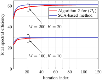
((a)) SEmax (i.e. $(\mathcal{P}_{1})$)

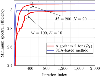
((b)) Max-min fairness (i.e. $(\mathcal{P}_{4})$)

Figure 1: Total SE and the minimum SE versus the number of iterations. The values of $M$ and $K$ are given explicitly the figure. Each AP is equipped with a single antenna.

In particular, Figs. 1(a) and 1(b) show the convergence of Algorithm 2 and the SCA-based method for the total spectral efficiency and the min-rate maximization problem, respectively. We can see that Algorithm 2 and SCA-based methods achieve the same performance but the SCA-based method requires fewer iterations to return a solution. However, the main advantage of Algorithm 2 over the SCA-based method is that each iteration of the proposed method is very memory efficient and can be done by closed-form expressions, and hence, is executed very fast. As a result, the total run-time of the proposed method is far less than that of the SCA-based method as shown in Table I. In Table I, we report the actual run-time of both methods to solve the SEmax problem. Here, we execute our codes on a 64-bit Windows operating system with 16 GB RAM and Intel CORE i7, 3.7 GHz. Both iterative methods are terminated when the difference of the objective for the last $5$ iterations is less than $10^{-3}$.

TABLE I: Comparison of run-time (in seconds) between Algorithm 2 and the SCA-based method for solving the SEmax problem. The values of other parameters are taken as $K=40,N=1$ and $D=1$.

number of APs	SCA-based method	Algorithm 2
200	330.84	2.88
400	408.94	9.42
800	1115.18	18.07
1600	1648.09	49.45

We next take advantage of the proposed methods to explore the spectral efficiency performance of large-scale cell-free massive MIMO that can cover, e.g. a large metropolitan area in our vision. In particular, we investigate the performance of cell-free massive MIMO for two cases $D=1$ and $D=10$. To obtain a fair comparison, we keep the AP density (defined as the number of APs per square kilometer) same for both cases. Note that the AP density of $1000$ means there are $10\,000$ APs for the case of $D=10$, which has not been studied in the literature previously. To appreciate the proposed method for this large-scale scenario, we compare it with the SCA method and the equal power allocation (EPA) method where the power control coefficient $\eta_{mk}$ is given by, $\eta_{mk}=(\sum_{i=1}^{k}\nu_{mi})^{-1}$. The results in Fig. 2 are interesting. First, increasing the AP density expectedly improves the total spectral efficiency of the system. Second, for the same AP density, a larger area provides a better sum spectral efficiency. The reason is that for a larger area, the users that are served by the APs become far apart each other. As a result, the inter-user inference becomes weaker, leading to an improved sum spectral efficiency. On the other hand, the EPA method yields smaller spectral efficiency as the coverage area is larger because more power should be to spent to the users having small path loss. The SCA-based method produces the same spectral efficiency as the proposed APG method but it is unable to run for $D=10$ on the system specifications mentioned above. Thus, the proposed scheme outperforms both SCA-based and the EPA methods in terms of sum spectral efficiency and coverage area.

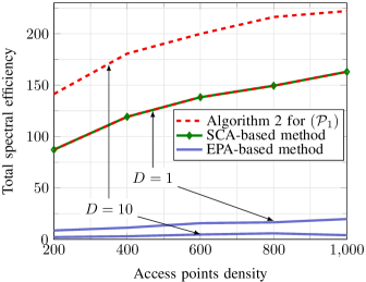
Figure 2: Total spectral efficiency versus AP density. The number of users is $K=40$.

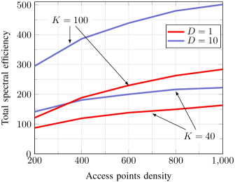
Figure 3: Total spectral efficiency versus AP density and number of users.

In Fig. 3, we again investigate the spectral efficiency performance of the AP density but for different number of users (i.e. $K=100$ and $K=40$). It can be seen that for a given AP density, the SE is increased if the number of users becomes larger. The gain is more profound for larger AP density due to the fact that more APs allow for more efficient exploitation of multiuser diversity gains.

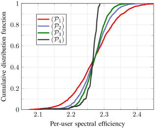
((a)) Small-scale problem: $K=20$ and $M=100$

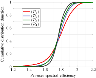
((b)) Large-scale problem: $K=500$ and $M=2000$

Figure 4: CDF of per-user spectral efficiency for $(\mathcal{P}_{1})$-$(\mathcal{P}_{4})$ for small scale and large-scale problems.

Next we plot the cumulative distribution function (CDF) of the per-user SE obtained by the four considered utility functions. Two settings are examined: $M=100$, $K=20$, $T_{c}=200$ symbols and $T_{p}=20$ symbols (cf. Fig. 4(a)), and $M=500$, $K=2000$, $T_{c}=1000$ and $T_{p}=200$ (cf. Fig. 4(b)). We can observe in Fig. 4 that the median values of the total achieved SEs are more or less the same for all the four utility functions. The $95\%$-likely achievable downlink SE is decreasing from $(\mathcal{P}_{1})$ to $(\mathcal{P}_{4})$ which can be explained by the fact that the following inequality holds: $\mathrm{SE}^{(\mathcal{P}_{1})}>\mathrm{SE}^{(\mathcal{P}_{2})}>\mathrm{SE}^{(\mathcal{P}_{3})}>\mathrm{SE}^{(\mathcal{P}_{4})}$, where $\mathrm{SE}^{(\mathcal{P}_{i})}$ denotes the per-user spectral efficiency obtained by solving $(\mathcal{P}_{i})$ [20]. It is also known that the order is reversed in terms of fairness. Consequently, the CDF of the per-user SE of $(\mathcal{P}_{4})$ (i.e. the MRmax problem) has the steepest slope and that of the SEmax problem is more spread. It is particularly interesting to see that the difference on the CDF of the per-user SE of all four utility metrics is marginal for large-scale cell-free massive MIMO. This simulation result again confirms that cell-free massive MIMO can deliver universally good services to all users in the system.

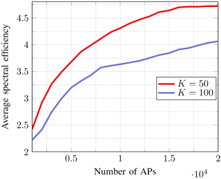
Figure 5: Average spectral efficiency versus number of APs for $K=100$ and $K=50$ users for $D=1$.

In the next experiment, we investigate how the average SE varies as a function of the number of APs. In particular, Fig. 5 shows the average spectral efficiency as a function of the number of APs for $K=100$ and $K=50$ users in an area of $D=1$. We can see that the average SE increases quickly when the number of APs is less 1000 for both $K=50$ and $K=100$ users, and it starts to saturate when the number of APs is larger. The reason is that for a given user, there should be a certain number of APs (i.e closest APs) that truly provides macro diversity gains to that user in terms of SE. Thus, a user may be served by a subset of APs to achieve similar SE performance. This can help reduce the overhead in cell-free massive MIMO. Further insights into this are discussed in the next numerical experiment.

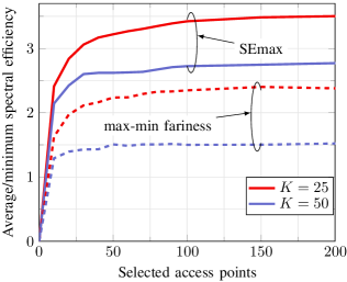
Figure 6: Average spectral efficiency versus number of selected APs for for $M=500$ and $D=1$.

In Fig. 6, we consider a scenario with $M=500$ APs and study how many APs are effectively required for each user. In particular, we plot the average spectral efficiency as a function of the number of selected APs per user for two utility functions: SEmax and MRmax. For a given user, a number of APs is simply selected based on their large-scale fading coefficients. From Fig. 6, we can observe that not all 500 APs are needed to serve 25 or 50 users in an area of $1\text{\,}{\mathrm{km}}^{2}$. Instead a smaller number of APs per user can can yield nearly the same performance. For example, we only need to assign less than $100$ APs to a user to achieve $95\%$ of the SE of the full system.

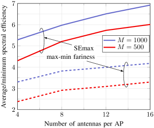
Figure 7: Average spectral efficiency with respect to the number of antenna at each AP for $K=50,D=1.$

Finally, we investigate the effect of increasing the number of antennas per AP on the sum SE and minimum SE. Specifically, we plot the average SE and minimum SE with respect to the number of antennas for both $M=500$ and $M=1000$ APs. The number of users is fixed to $K=50$. Expectedly, the SE increases with the increase in the number of antennas per APs but the increase tends to be small when the number of antennas is sufficiently large. The reason is that for a large number of APs channel harderning and favorable propagation can be achieved by a few antennas per AP. Specifically, we can see that the SE for the case of $1000$ APs and $4$ antennas per AP is larger than the SE for the case of 500 APs and 8 antennas per AP. Therefore, for large-scale cell-free massive MIMO, having more APs with a few antennas each seems to be more beneficial than having fewer APs with more antennas each.

VI Conclusion

We have considered the downlink of cell-free massive MIMO and aimed to maximize four utility functions, subject to a power constraint at each AP. Conjugate beamforming has been adopted, resulting in a power control problem for which an accelerated project gradient method has been proposed. Particularly, the proposed solutions only requires the first order information of the objective and, in particular, each iteration of the proposed solutions can be computed by closed-form expressions. We have numerically shown that the proposed methods can achieve (nearly) the same SE as a known SCA-based method but with much lesser run time. For the first time, we have evaluated the SE performance of cell-free massive MIMO for an area of $10\text{\,}{\mathrm{km}}^{2}$, consisting of up to $10\,000$ APs, whereby the achieved SE can be up to 200 (bit/s/Hz). We have also found that the SE performance of the four utility functions is quite similar for large-scale cell-free massive MIMO, confirming again that cell-free massive MIMO can provide uniformed services to all users.

-A Solution to the Projection onto $\mathcal{S}$

The solution of (28) can be found using the KKT conditions given by

$$\nabla_{\boldsymbol{\mu}_{m}}\mathcal{L}=2(\boldsymbol{\mu}_{m}-\mathbf{x}_{m})+2\lambda\boldsymbol{\mu}_{m} =0,$$ (45a)

$$\lambda(||\boldsymbol{\mu}_{m}||^{2}-\frac{1}{N}) =0,$$ (45b)

$$||\boldsymbol{\mu}_{m}||^{2} \leq\frac{1}{N},$$ (45c)

$$\lambda \geq 0.$$ (45d)

Applying the constraint $\boldsymbol{\mu}_{m}\geq 0$ to (45a), we get

$$\mathbf{x}_{m}=(1+\lambda)\boldsymbol{\mu}_{m}\geq 0.$$ (46)

If $\lambda=0$, the stationary condition in (45a) results in

$$\boldsymbol{\mu}_{m}=\mathbf{x}_{m},$$ (47)

and (45c) gives $\boldsymbol{\mu}_{m}=\mathbf{x}_{m}\leq\frac{1}{N}$, which corresponds to the case where $\mathbf{x}_{m}$ lies in $\mathcal{S}$. If $\lambda>0$, the complementary slackness in (45b) implies that $||\boldsymbol{\mu}_{m}||^{2}=\frac{1}{N}$. The equality in (46) can further be written as

$$\boldsymbol{\mu}_{m}^{\mbox{\scriptsize T}}\mathbf{x}_{m} =(1+\lambda)\boldsymbol{\mu}_{m}^{\mbox{\scriptsize T}}\boldsymbol{\mu}_{m}=(1+\lambda)\frac{1}{N}.$$ (48)

Since $\lambda>0$, we get $N\boldsymbol{\mu}_{m}^{\mbox{\scriptsize T}}\mathbf{x}_{m}-1>0$ or $\boldsymbol{\mu}_{m}^{\mbox{\scriptsize T}}\mathbf{x}_{m}>\frac{1}{N}$. By using the Cauchy–Schwartz inequality, we can write $||\boldsymbol{\mu}_{m}||\,||\mathbf{x}_{m}||>\frac{1}{N}$ or $||\mathbf{x}_{m}||^{2}>\frac{1}{N}$, which refers to the case where $\mathbf{x}_{m}$ lies outside $\mathcal{S}$. Furthermore, substituting $\lambda=N\boldsymbol{\mu}_{m}^{\mbox{\scriptsize T}}\mathbf{x}_{m}-1$ into (46), we get

$$\mathbf{x}_{m}=N(\boldsymbol{\mu}_{m}^{\mbox{\scriptsize T}}\mathbf{x}_{m})\boldsymbol{\mu}_{m},$$ (49)

which means that $\boldsymbol{\mu}_{m}$ is parallel to $\mathbf{x}_{m}$ or $\boldsymbol{\mu}_{m}=a\mathbf{x}_{m}$ where $a$ is a constant. Next using (49) gives $a=\frac{1/\sqrt{N}}{||\mathbf{x}_{m}||^{2}}$ and therefore

$$\boldsymbol{\mu}_{m}=\frac{1/\sqrt{N}}{||\mathbf{x}_{m}||^{2}}\mathbf{x}_{m}.$$ (50)

Combining (46), (47) and (50) results in

$$\mu_{m}=\frac{\sqrt{1/N}}{\max\left(\sqrt{1/N},||[\mathbf{x}_{m}]_{+}||\right)}[\mathbf{x}_{m}]_{+},$$ (51)

which completes the proof.

-B Lipschitz Constant of $\nabla f(\boldsymbol{\mu})$

Assessing the Lipschitz constant of $\nabla f(\boldsymbol{\mu})$ for the four problems discussed in the paper boils down to finding the Lipschitz constant of $\nabla\mathrm{SE}_{k}(\boldsymbol{\mu})$. A convenient way to do this is to rewrite the function $\mathrm{SE}_{k}(\boldsymbol{\mu})$ in the form of single variable $\boldsymbol{\mu}$ which can be done by denoting $\mathbf{A}_{i}\triangleq\mathbf{I}_{M}\otimes\mathbf{e}_{i}^{\mbox{\scriptsize T}}$. Then, we can write $\bar{\boldsymbol{\mu}}_{i}$ as $\mathbf{A}_{i}\boldsymbol{\mu}$, and thus $\gamma_{k}(\boldsymbol{\mu})$, the SINR of the $k$-th user, can be rewritten as

$$\gamma_{k}(\boldsymbol{\mu})=\frac{\overbrace{\zeta_{d}(\bar{\boldsymbol{\nu}}_{kk}^{\mbox{\scriptsize T}}\mathbf{A}_{k}\boldsymbol{\mu})^{2}}^{b_{k}(\boldsymbol{\mu})}}{\underbrace{\zeta_{d}\left(\sum_{i\neq k}^{K}(\bar{\boldsymbol{\nu}}_{ik}^{\mbox{\scriptsize T}}\mathbf{A}_{i}\boldsymbol{\mu})^{2}+\frac{1}{N}\sum_{i=1}^{K}||\bar{\mathbf{D}}_{k}\mathbf{A}_{i}\boldsymbol{\mu}||_{2}^{2}\right)}_{c_{k}(\boldsymbol{\mu})}+\frac{1}{N^{2}}}.$$ (52)

The gradient of $\mathrm{SE}_{k}(\boldsymbol{\mu})$ with respect to $\boldsymbol{\mu}$ is found as

$$\nabla\mathrm{SE}_{k}(\boldsymbol{\mu})=\nabla_{\boldsymbol{\mu}}\log(1+\gamma_{k}(\boldsymbol{\mu}))=\frac{\nabla_{\boldsymbol{\mu}}\left(b_{k}(\boldsymbol{\mu})+c_{k}(\boldsymbol{\mu})\right)}{b_{k}(\boldsymbol{\mu})+c_{k}(\boldsymbol{\mu})+\frac{1}{N^{2}}}-\frac{\nabla_{\boldsymbol{\mu}}c_{k}(\boldsymbol{\mu})}{c_{k}(\boldsymbol{\mu})+\frac{1}{N^{2}}},$$ (53)

where $\nabla_{\boldsymbol{\mu}}b(\boldsymbol{\mu})$ and $\nabla_{\boldsymbol{\mu}}c(\boldsymbol{\mu})$ are given by

$$\nabla_{\boldsymbol{\mu}}b_{k}(\boldsymbol{\mu})=2\zeta_{d}\mathbf{A}_{k}^{\mbox{\scriptsize T}}\bar{\boldsymbol{\nu}}_{kk}\bar{\boldsymbol{\nu}}_{kk}^{\mbox{\scriptsize T}}\mathbf{A}_{k}\boldsymbol{\mu},$$ (54)

$$\nabla_{\boldsymbol{\mu}}c_{k}(\boldsymbol{\mu})=2\zeta_{d}\left(\sum_{i\neq k}^{K}\mathbf{A}_{i}^{\mbox{\scriptsize T}}\bar{\boldsymbol{\nu}}_{ik}\bar{\boldsymbol{\nu}}_{ik}^{\mbox{\scriptsize T}}\mathbf{A}_{i}+\frac{1}{N}\sum_{i=1}^{K}\mathbf{A}_{i}^{\mbox{\scriptsize T}}\bar{\mathbf{D}}_{k}^{2}\mathbf{A}_{i}\right)\boldsymbol{\mu}.$$ (55)

Now the Lipschitz continuity of $\nabla_{\boldsymbol{\mu}}b_{k}(\boldsymbol{\mu})$ and $\nabla_{\boldsymbol{\mu}}c_{k}(\boldsymbol{\mu})$ is obvious, and so is that of $\nabla\mathrm{SE}_{k}(\boldsymbol{\mu})$. Although we can compute the Lipschitz constant of $\nabla\mathrm{SE}_{k}(\boldsymbol{\mu})$, this is quite involved and not necessary since a line search is used to find a proper step size.

-C Convergence Proof of Algorithm 1

The proof is due to [18]. First, we note that since $\nabla f(\boldsymbol{\mu})$ is Lipschitz continuous and a line search is used to find a proper step size in Algorithm 2, it is sufficient to prove the convergence Algorithm 1. We begin with by recalling an important inequality of a $L$-smooth function. Specifically, for a function $f(\mathbf{x})$ has the Lipschitz continuous gradient with a constant $L_{f}$, the following inequality holds

$$f(\mathbf{y})\geq f(\mathbf{x})+\bigl{\langle}\nabla f\bigl{(}\mathbf{x}\bigr{)},\mathbf{y}-\mathbf{x}\bigr{\rangle}-\frac{L_{f}}{2}||\mathbf{y}-\mathbf{x}||^{2}.$$ (56)

The projection in Step 6 of Algorithm 1 can be written as

$$\mathbf{v}^{n+1}=\underset{\boldsymbol{\mu}\in\mathcal{S}}{\arg\min}\bigl{\|}\boldsymbol{\mu}-\boldsymbol{\mu}^{n}-\alpha\nabla f\bigl{(}\boldsymbol{\mu}^{n}\bigr{)}\bigr{\|}^{2}=\underset{\boldsymbol{\mu}\in\mathcal{S}}{\arg\max}\ \bigl{\langle}\nabla f\bigl{(}\boldsymbol{\mu}^{n}\bigr{)},\boldsymbol{\mu}-\boldsymbol{\mu}^{n}\bigr{\rangle}-\frac{1}{2\alpha}||\boldsymbol{\mu}-\boldsymbol{\mu}^{n}||^{2},$$ (57)

where we have used the fact that $||\mathbf{a}-\mathbf{b}||^{2}=||\mathbf{a}||^{2}+||\mathbf{b}||^{2}+2\left\langle\mathbf{a},\mathbf{b}\right\rangle$. Note that when $\boldsymbol{\mu}=\boldsymbol{\mu}^{n}$, the objective in the above problem is $0$, and thus we have

$$\bigl{\langle}\nabla f\bigl{(}\boldsymbol{\mu}^{n}\bigr{)},\mathbf{v}^{n+1}-\boldsymbol{\mu}^{n}\bigr{\rangle}-\frac{1}{2\alpha}||\mathbf{v}^{n+1}-\boldsymbol{\mu}^{n}||^{2}\geq 0.$$ (58)

Applying (56) yields

$$f(\mathbf{v}^{n+1}) \geq f\bigl{(}\boldsymbol{\mu}^{n}\bigr{)}+\bigl{\langle}\nabla f\bigl{(}\boldsymbol{\mu}^{n}\bigr{)},\mathbf{v}^{n+1}-\boldsymbol{\mu}^{n}\bigr{\rangle}-\frac{L_{f}}{2}\bigl{\|}\mathbf{v}^{n+1}-\boldsymbol{\mu}^{n}\bigr{\|}^{2}$$

$$\geq f\bigl{(}\boldsymbol{\mu}^{n}\bigr{)}+\bigl{(}\frac{1}{2\alpha}-\frac{L_{f}}{2}\bigr{)}\bigl{(}\bigl{\|}\mathbf{v}^{n+1}-\boldsymbol{\mu}^{n}\bigr{\|}^{2}.$$ (59)

It is easy to see that $f(\mathbf{v}^{n+1})\geq f\bigl{(}\boldsymbol{\mu}^{n}\bigr{)}$ if $\alpha<\frac{1}{L_{f}}$. From Step 7, if $f(\mathbf{z}^{n+1})\geq f(\mathbf{v}^{n+1})$, then

$$\boldsymbol{\mu}^{n+1} =\mathbf{z}^{n+1},f\bigl{(}\boldsymbol{\mu}^{n+1}\bigr{)}=f(\mathbf{z}^{n+1})\geq f(\mathbf{v}^{n+1}).$$ (60)

Similar if $f(\mathbf{z}^{n+1})<f(\mathbf{v}^{n+1})$, then

$$\boldsymbol{\mu}^{n+1} =\mathbf{v}^{n+1},f\bigl{(}\boldsymbol{\mu}^{n+1}\bigr{)}=f(\mathbf{v}^{n+1}).$$ (61)

From (59), (60), and (61) we have

$$f\bigl{(}\boldsymbol{\mu}^{n+1}\bigr{)}\geq f(\mathbf{v}^{n+1})\geq f\bigl{(}\boldsymbol{\mu}^{n}\bigr{)}.$$ (62)

Since the feasible set of the considered problems is compact convex, the iterates $\{\mathbf{v}^{n}\}$ and $\{\boldsymbol{\mu}^{n}\}$ are both bounded and thus $\{\boldsymbol{\mu}^{n}\}$ has accumulation points. As shown above, $f\bigl{(}\boldsymbol{\mu}^{n}\bigr{)}$ is nondecreasing, $f$ has the same value, denoted by $f^{\ast}$, at all the accumulation points. From (59), we have

$$f\bigl{(}\boldsymbol{\mu}^{n+1}\bigr{)}-f\bigl{(}\boldsymbol{\mu}^{n}\bigr{)}\geq f(\mathbf{v}^{n+1})-f\bigl{(}\boldsymbol{\mu}^{n}\bigr{)}\geq\bigl{(}\frac{1}{2\alpha}-\frac{L_{f}}{2}\bigr{)}\bigl{(}\bigl{\|}\mathbf{v}^{n+1}-\boldsymbol{\mu}^{n}\bigr{\|}^{2},$$ (63)

which results in

$$\infty>f^{\ast}-f\bigl{(}\boldsymbol{\mu}^{1}\bigr{)}\geq\sum_{n=1}^{\infty}\bigl{(}\frac{1}{2\alpha}-\frac{L_{f}}{2}\bigr{)}\bigl{(}\bigl{\|}\mathbf{v}^{n+1}-\boldsymbol{\mu}^{n}\bigr{\|}^{2}.$$ (64)

Since $\alpha<\frac{1}{L_{f}}$, we can conclude that

$$\bigl{\|}\mathbf{v}^{n+1}-\boldsymbol{\mu}^{n}\bigr{\|}\to 0\ \textrm{as}\ n\to\infty.$$ (65)

The convergence proof of Algorithm 1 to a critical point of $(\mathcal{P}_{1})$ follows the same arguments as those in [18] and thus, is omitted for the sake of brevity.

References

- [1] M. Farooq, Q. H. Ngo, and L.-N. Tran, “Accelerated projected gradient method for the optimization of cell-free massive mimo downlink,” in Proc. IEEE PIMRC 2020, 2020, to appear.
- [2] E. Telatar, “Capacity of multi-antenna Gaussian channels,” Eur. Trans. Telecommun, vol. 10, pp. 585–598, Nov. 1999.
- [3] G. J. Foschini and M. J. Gans, “On limits of wireless communications in a fading environment when using multiple antennas,” Wireless Pers.Commun, vol. 6, pp. 311–335, Mar. 1998.
- [4] S. Alamouti, “A simple transmit diversity technique for wireless communications,” IEEE J. Select. Areas Commun., vol. 16, no. 8, pp. 1451–1458, Oct. 1998.
- [5] T. L. Marzetta, “Noncooperative cellular wireless with unlimited numbers of base station antennas,” IEEE Trans. Wireless Commun., vol. 9, no. 11, pp. 3590–3600, November 2010.
- [6] F. Boccardi, R. W. Heath, A. Lozano, T. L. Marzetta, and P. Popovski, “Five disruptive technology directions for 5G,” IEEE Commun. Mag., vol. 52, no. 2, pp. 74–80, February 2014.
- [7] E. Dahlman, S. Parkvall, and J. Skold, 5G NR: The Next Generation Wireless Access Technology, 1st ed. Academic Press, 2018.
- [8] A. Lozano, R. W. Heath, and J. G. Andrews, “Fundamental limits of cooperation,” IEEE Trans. Inform. Theory, vol. 59, no. 9, pp. 5213–5226, Sep. 2013.
- [9] H. Yang and T. L. Marzetta, “A macro cellular wireless network with uniformly high user throughputs,” in 2014 IEEE 80th Vehicular Technology Conference (VTC2014-Fall), 2014.
- [10] E. Björnson, L. Sanguinetti, H. Wymeersch, J. Hoydis, and T. L. Marzetta, “Massive MIMO is a reality – What is next? Five promising research directions for antenna arrays,” Digital Signal Processing, vol. 94, pp. 3–20, 2019, Special Issue on Source Localization in Massive MIMO. [Online]. Available: http://www.sciencedirect.com/science/article/pii/S1051200419300776
- [11] H. Q. Ngo, A. Ashikhmin, H. Yang, E. G. Larsson, and T. L. Marzetta, “Cell-free massive MIMO versus small cells,” IEEE Trans. Wireless Commun., vol. 16, no. 3, pp. 1834–1850, March 2017.
- [12] H. Q. Ngo, L.-N. Tran, T. Q. Duong, M. Matthaiou, and E. G. Larsson, “On the total energy efficiency of cell-free massive MIMO,” IEEE Transactions on Green Communications and Networking, vol. 2, no. 1, pp. 25–39, March 2018.
- [13] J. Zhang, S. Chen, Y. Lin, J. Zheng, B. Ai, and L. Hanzo, “Cell-free massive MIMO: A new next-generation paradigm,” IEEE Access, vol. 7, pp. 99 878–99 888, 2019.
- [14] Z. Chen and E. Björnson, “Channel hardening and favorable propagation in cell-free massive MIMO with stochastic geometry,” IEEE Trans. Commun., vol. 66, no. 11, pp. 5205–5219, 2018.
- [15] L. D. Nguyen, T. Q. Duong, H. Q. Ngo, and K. Tourki, “Energy efficiency in cell-free massive MIMO with zero-forcing precoding design,” IEEE Commun. Lett., vol. 21, no. 8, pp. 1871–1874, Aug 2017.
- [16] S. Buzzi and A. Zappone, “Downlink power control in user-centric and cell-free massive MIMO wireless networks,” in IEEE PIMRC, Oct 2017, pp. 1–6.
- [17] G. Interdonato, H. Q. Ngo, P. Frenger, and E. G. Larsson, “Downlink training in cell-free massive MIMO: A blessing in disguise,” IEEE Trans. Wireless Commun., 2019, in Press.
- [18] H. Li and Z. Lin, “Accelerated proximal gradient methods for nonconvex programming,” in Advances in Neural Information Processing Systems 28, C. Cortes, N. D. Lawrence, D. D. Lee, M. Sugiyama, and R. Garnett, Eds. Curran Associates, Inc., 2015, pp. 379–387.
- [19] L.-N. Tran and H. Q. Ngo, “First-order methods for energy-efficient power control in cell-free massive MIMO,” in 53rd Asilomar Conference on Signals, Systems, and Computers, 2019, pp. 848–852.
- [20] Z.-Q. Luo and S. Zhang, “Dynamic spectrum management: Complexity and duality,” IEEE J. Sel. Topics Signal Process., vol. 2, no. 1, pp. 57–73, Feb. 2008.
- [21] H. H. Bauschke, M. N. Bui, and X. Wang, “Projecting onto the intersection of a cone and a sphere,” SIAM Journal on Optimization, vol. 28, no. 3, pp. 2158–2188, Jan 2018.
- [22] Y. Nesterov, “Smooth minimization of non-smooth functions,” Math. Program., Ser. A, vol. 103, pp. 127–152, 2005.
- [23] A. Ben-Tal and A. Nemirovski, Lectures on Modern Convex Optimization. Society for Industrial and Applied Mathematics, 2001. [Online]. Available: https://epubs.siam.org/doi/abs/10.1137/1.9780898718829
- [24] M. ApS, The MOSEK optimization toolbox for MATLAB manual. Version 7.1 (Revision 28)., 2015.
- [25] J. Löfberg, “YALMIP : A toolbox for modeling and optimization in MATLAB,” in Proc. the CACSD Conference, 2004.