Beyond Individualized Recourse: Interpretable and Interactive Summaries of Actionable Recourses
Abstract
As predictive models are increasingly being deployed in high-stakes decision-making, there has been a lot of interest in developing algorithms which can provide recourses to affected individuals. While developing such tools is important, it is even more critical to analyse and interpret a predictive model, and vet it thoroughly to ensure that the recourses it offers are meaningful and non-discriminatory before it is deployed in the real world. To this end, we propose a novel model agnostic framework called Actionable Recourse Summaries (AReS) to construct global counterfactual explanations which provide an interpretable and accurate summary of recourses for the entire population. We formulate a novel objective which simultaneously optimizes for correctness of the recourses and interpretability of the explanations, while minimizing overall recourse costs across the entire population. More specifically, our objective enables us to learn, with optimality guarantees on recourse correctness, a small number of compact rule sets each of which capture recourses for well defined subpopulations within the data. We also demonstrate theoretically that several of the prior approaches proposed to generate recourses for individuals are special cases of our framework. Experimental evaluation with real world datasets and user studies demonstrate that our framework can provide decision makers with a comprehensive overview of recourses corresponding to any black box model, and consequently help detect undesirable model biases and discrimination.
1 Introduction
Over the past decade, machine learning (ML) models are being increasingly deployed to make a variety of consequential decisions ranging from hiring decisions to loan approvals. Consequently, there is growing emphasis on designing tools and techniques which can explain the decisions of these models to the affected individuals and provide a means for recourse [38]. For example, when an individual is denied loan by a credit scoring model, he/she should be informed about the reasons for this decision and what can be done to reverse it. Several approaches in recent literature tackled the problem of providing recourses to affected individuals by generating local (instance level) counterfactual explanations [39, 36, 12, 27, 20]. For instance, Wachter et al. [39] proposed a model-agnostic, gradient based approach to find a closest modification (counterfactual) to any data point which can result in the desired prediction.
While prior research has focused on providing counterfactual explanations (recourses) for individual instances, it has left a critical problem unadressed. It is often important to analyse and interpret a model, and vet it thoroughly to ensure that the recourses it offers are meaningful and non-discriminatory before it is deployed in the real world. To achieve this, appropriate stake holders and decision makers should be provided with a high level, global understanding of model behaviour. However, existing techniques cannot be leveraged here as they are only capable of auditing individual instances. Consequently, while existing approaches can be used to provide recourses to affected individuals after a model is deployed, they cannot assist decision makers in deciding if a model is good enough to be deployed in the first place.
Contributions: In this work, we propose a novel model agnostic framework called Actionable Recourse Summaries (AReS) to learn global counterfactual explanations which can provide an interpretable and accurate summary of recourses for the entire population with emphasis on specific subgroups of interest. These subgroups can be characterized either by specific features of interest input by an end user (e.g., race, gender) or can be automatically discovered by our framework. The goal of our framework is to enable decision makers to answer big picture questions about recourse–e.g.,how does the recourse differ across various racial subgroups?. To the best of our knowledge, this is the first work to address the problem of providing accurate and interpretable summaries of recourses which in turn enable decision makers to answer the aforementioned big picture questions.
To construct the aforementioned explanations, we formulate a novel objective function which simultaneously optimizes for correctness of the recourses and interpretability of the resulting explanations, while minimizing the overall recourse costs across the entire population. More specifically, our objective enables us to learn, with optimality guarantees on recourse correctness, a small number of compact rule sets each of which capture recourses for well defined subpopulations within the data. We also demonstrate theoretically that several of the prior approaches proposed to generate recourses for individuals are special cases of our framework. Furthermore, unlike prior research, we do not make the unrealistic assumption that we have access to real valued recourse costs. Instead, we develop a framework which leverages Bradley-Terry model to learn these costs from pairwise comparisons of features provided by end users.
We evaluated the effectiveness of our framework on three real world datasets: credit scoring, judicial bail decisions, and recidivism prediction. Experimental results indicate that our framework outputs highly interpretable and accurate global counterfactual explanations which serve as concise overviews of recourses. Furthermore, while the primary goal of our framework is to provide high level overviews of recourses, experimental results demonstrate that our framework performs on par with state-of-the-art baselines when it comes to providing (instance level) recourses to affected individuals. Lastly, results from a user study we carried out suggest that human subjects are able to detect biases and discrimination in recourses very effectively using the explanations output by our framework.
Related Work: A variety of post hoc techniques have been proposed to explain complex models [8, 30, 15]. For instance, LIME [29] and SHAP [23], are model-agnostic, local explanation approaches which learn a linear model locally around each prediction. Other local explanation methods capture feature importances by computing the gradient with respect to the input [32, 34, 31, 33]. An alternate approach is to provide a global explanation summarizing the black box as a whole [17, 3], typically using an interpretable model. However, none of the aforementioned techniques were designed to learn counterfactual explanations or provide recourse.
Several approaches in recent literature addressed the problem of providing recourses to affected individuals by learning local counterfactual explanations for binary classification models [39, 27, 12, 36]. The main idea behind all these approaches is to determine what is the most desirable change that can be made to an individual’s feature vector to reverse the obtained predictionDandl et al. [7]. Counterfactual explanations have also been leveraged to help in unsupervised exploratory data analysis of datasets in low dimensional latent spaces [26]. Wachter et al. [39], the initial proponents of counterfactual explanations for recourse, used gradient based optimization to search for the closest counterfactual instance to a given data point. Other approaches utilized standard SAT solvers [12], explanations output by methods such as SHAP [28], the perturbations in latent space found by autoencoders [25, 11], or the inherent structures of tree-based models [35, 22] to generate recourses.
More recent work focused on ensuring that the recourses being found were actionable. While Ustun et al. [36] proposed an efficient integer programming approach to obtain actionable recourses for linear classifiers, few other approaches focused on actionable recourses for tree based ensembles [35, 22]. Furthermore, Looveren and Klaise [20] and Poyiadzi et al. [27] proposed methods for obtaining more realistic counterfactuals by either prioritizing counterfactuals similar to certain class prototypes or ensuring that the path between the counterfactual and the original instance is one of high kernel density. Another way to build feasibility into counterfactual explanations is to suggest multiple counterfactuals for each data point, as done by Mothilal et al. [24] using gradient descent and Dandl et al. [7] using genetic algorithms. Although there are diverse techniques for finding counterfactual explanations, using these as recourses in the real-world is non-trivial since this involves making causal assumptions that may be violated when minimising recourse costs [13, 2, 37].
It is important to note that none of the aforementioned approaches provide a high level, global understanding of recourses which can be used by decision makers to vet the underlying models. Ours is the first work to address this problem by providing accurate and interpretable summaries of actionable recourses.
2 Our Framework: Actionable Recourse Summaries
Here, we describe our framework, Actionable Recourse Summaries (AReS), which is designed to learn global counterfactual explanations which provide an interpretable and accurate summary of recourses for the entire population. Below, we discuss in detail: 1) the representation that we choose to construct our explanations, 2) how we quantify the notions of fidelity, interpretability, and costs associated with recourses, 3) our objective function and its characteristics, 4) theoretical results demonstrating that our framework subsumes several of the previously proposed recourse generation approaches and, 5) optimization procedure with theoretical guarantees on recourse correctness.
2.1 Our Representation: Two Level Recourse Sets
The most important criterion for choosing a representation is that it should be understandable to decision makers who are not experts in machine learning, approximate complex non-linear decision surfaces accurately, and allow us to easily incorporate user preferences. To this end, we propose a new representation called two level recourse sets which builds on the previously proposed two level decision sets [17]. Below, we define this representation formally.
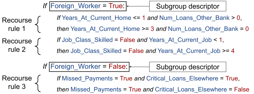
A recourse rule is a tuple embedded within an if-then structure i.e., “if , then ”. and are conjunctions of predicates of the form “”, where is an operator (e.g., ). Furthermore, there are two constraints that need to be satisfied by and : 1) the corresponding features in and should match exactly and, 2) there should be at least one change in the values and/or operators between and . A recourse rule intuitively captures the current state () of an individual or a group of individuals, and the changes required to the current state () to obtain a desired prediction. Figure 1 shows examples of recourse rules. A recourse set is a set of unordered recourse rules i.e., .
A two level recourse set is a hierarchical model consisting of multiple recourse sets each of which is embedded within an outer if-then structure (Figure 1). Intuitively, the outer if-then rules can be thought of as subgroup descriptors which correspond to different subpopulations within the data, and the inner if-then rules are recourses for the corresponding subgroups. Formally, a two-level recourse set is a set of triples and has the following form: where corresponds to the subgroup descriptor, and together represent the inner if-then recourse rules with denoting the antecedent (i.e., the if condition) and denoting the consequent (i.e., the recourse). A two level recourse set can be used to provide a recourse to an instance as follows: if satisfies exactly one of the rules i.e., satisfies , then its recourse is . If satisfies none of the rules in , then is unable to provide a recourse to . If satisfies more than one rule in , then its recourse is given by the rule that has the highest probability of providing a correct recourse. Note that this probability can be computed directly from the data. Other forms of tie-breaking functions can be easily incorporated into our framework.
| Recourse Correctness | incorrectrecourse |
|---|---|
| Recourse Coverage | cover |
| Recourse Costs | featurecost; featurechange |
| Interpretability | size number of triples in ; maxwidth |
| numrsets |
2.2 Quantifying Recourse Correctness, Coverage, Costs, and Interpretability
To correctly summarize recourses for various subpopulations of interest, it is important to construct an explanation that not only accounts for the correctness of recourses, but also provides recourses to as many affected individuals as possible, minimizes recourse costs, and is interpretable. Below we explore each of these desiderata in detail and discuss how to quantify them w.r.t a two level recourse set with triples, a black box model , and a dataset where captures the feature values of instance . We treat the black box model as a function which takes an instance as input and returns a class label–positive (1) or negative (0). We use to denote those instances for which i.e., denotes the set of affected individuals who have received unfavorable predictions from the black box model.
Recourse Correctness: The explanations that we construct should capture recourses accurately. More specifically, when we use the recourse rules outlined by our explanation to prescribe recourses to affected individuals, they should be able to obtain the desired predictions from the black box model upon acting on the recourse. To quantify this notion, we define incorrectrecourse which is defined as the number of instances in for which acting upon the recourse prescribed by does not result in the desired prediction (Table 1). Our goal would therefore be to construct explanations that minimize this metric.
Recourse Coverage: It is important to ensure that the explanation that we construct covers as many individuals as possible i.e., provides recourses to them. To quantify this notion, we define cover as the number of instances in which satisfy the condition associated with some rule in and are thereby provided a recourse by the explanation (Table 1).
Interpretability: The explanations that we output should be easy to understand and reason about. While choosing an interpretable representation (e.g., two level recourse sets) contributes to this, it is not sufficient to ensure interpretability. For example, while a decision tree with a hundred levels is technically readable by a human user, it cannot be considered as interpretable. Therefore, it is important to not only have an intuitive representation but also to achieve smaller complexity.
We quantify the interpretability of explanation using the following metrics: size() is the number of triples of the form in the two level recourse set . maxwidth() is the maximum number of predicates (e.g., age 50) in conjunctions computed over all triples of . numrsets() counts the number of unique subgroup descriptors (outer if-then clauses) in . All these metrics are formally defined in Table 1.
Recourse Costs: When constructing explanations, we also need to account for minimizing the recourse costs across the entire population. We define two metrics to quantify the recourse costs. First, we assume each feature is associated with a cost that captures how difficult it is to change that feature. This encapsulates the notion that some features are more actionable than the others. We define the total feature cost of a two-level recourse set , featurecost, as the sum of the costs of each of the features present in and whose value changes from to , computed across all triples of . Second, apart from feature costs, it is also important to account for reducing the magnitude of changes in feature values. For example, it is much easier to increase income by 5K than 50K. To capture this notion, we define featurechange as the sum of magnitude of changes in feature values from to , computed across all triples in . In case of categorical features, going from one value to another corresponds to a change of magnitude . Continuous features can be converted into ordinal features by binning the feature values. In this case, going from one bin to the next immediate bin corresponds to a change of magnitude . Other notions of magnitude can also be easily incorporated into our framework. Our goal would be construct explanations that minimize the aforementioned metrics. Table 1 captures the formal definitions of these metrics.
2.2.1 Learning Feature Costs from Pairwise Feature Comparisons
One of the biggest challenges of computing featurecost is that it is non-trivial to obtain costs that capture the difficulty associated with changing a feature. For instance, even experts would find it hard to put precise costs indicating how unactionable a feature is. On the other hand, it is relatively easy for experts to make pairwise comparisons between features and assess which features are easier to change [6]. For example, a expert would be able to easily identify that it is much harder to increase income compared to number of bank accounts for any customer. Furthermore, there might be some ambiguity when comparing certain pairs of features and experts might have different opinions about which features are more actionable (e.g., increasing income vs. buying a car). So, it is important to account for this uncertainty .
AReS requires as input a vector of costs representing the difficulty of changing each model feature. We propose to learn this probabilistically in order to account for the variation in the opinions of experts regarding actionability of features. It is important to note however that AReS, is flexible enough to support feature costs computed in any other manner, or even specified directly through user input. This customization makes our method more generic compared to other existing counterfactual methods.
The Bradley-Terry Model: We leverage pairwise feature comparison inputs to learn the costs associated with each feature. To this end, we employ the well known Bradley-Terry model [21, 4] which states: If is the probability that feature is less actionable (harder to change) compared to feature , then we can calculate this probability as where and correspond to the costs of features and respectively. Note that can be computed directly from the pairwise comparisons obtained by surveying experts, as . We can then retrieve the costs of the features by learning the MAP estimates of feature costs and [5, 10].
2.3 Learning Two Level Recourse Sets
We formulate an objective function that can jointly optimize for recourse correctness, coverage, costs, and interpretability of an explanation. We assume that we are given as inputs a dataset , a set of instances that received unfavorable predictions (i.e., labeled as ) from the black box model , a candidate set of conjunctions of predicates (e.g., age 50 and gender female) from which we can pick the subgroup descriptors, and another candidate set of conjunctions of predicates from which we can choose the recourse rules. In practice, a frequent itemset mining algorithm such as apriori [1] can be used to generate the candidate sets of conjunctions of predicates. If the user does not provide any input, both and are assigned to the same candidate set generated by apriori.
To facilitate theoretical analysis, the metrics defined in Table 1 are expressed in the objective function either as non-negative reward functions or constraints. To construct non-negative reward functions, penalty terms (metrics in Table 1) are subtracted from their corresponding upper bound values (, , ) which are computed with respect to the sets and .
where and denote the maximum possible feature cost and the maximum possible magnitude of change over all features respectively. These values are computed from the data directly. and are as described below. The resulting optimization problem is:
| (1) | |||
are non-negative weights which manage the relative influence of the terms in the objective. These can be specified by an end user or can be set using cross validation (details in experiments section). The values of are application dependent and need to be set by an end user.
Theorem 2.1.
The objective function in Eqn. 1 is non-normal, non-negative, non-monotone, submodular and the constraints of the optimization problem are matroids.
Proof (Sketch).
Non-negative functions and submodular functions are both closed under addition and multiplication with non-negative scalars. Each term is non-negative by construction. is submodular, and the remaining terms are modular (and therefore submodular). Since , the objective is submodular. To show that the objective is non-monotone, it suffices to show that is non-monotone for some . Let and be two explanations s.t. i.e., has at least as many recourse rules as . By definition, which implies that . Therefore, is non-monotone. See Appendix for a detailed proof. ∎
Theorem 2.2.
If all features take on values from a finite set, then the optimization problem in Eqn. 1 can be reduced to the objectives employed by prior approaches which provide instance level counterfactuals for individual recourse.
Proof (Sketch).
Individual recourse is represented in AReS by and having consist of the entire feature-vector of a particular data-point . Additonally setting ensures the generated triples represent instance level counterfactuals. Finally, setting hyperparameter values and leaves us with an objective function of , which performs the same recourse search for individual recourse as the objectives outlined in prior work [39, 12, 36]. See Appendix for a detailed proof. ∎
Optimization Procedure While exactly solving the optimization problem in Eqn. 1 is NP-Hard [14], the specific properties of the problem: non-monotonicity, submodularity, non-normality, non-negativity and the accompanying matroid constraints allow for applying algorithms with provable optimality guarantees. We employ an optimization procedure based on approximate local search [19] which provides the best known theoretical guarantees for this class of problems (Pseudocode for this procedure is provided in Appendix). More specifically, the procedure we employ provides an optimality guarantee of where is the number of constraints and .
Theorem 2.3.
If the underlying model provides recourse to all individuals, then upper bound on the proportion of individuals in for whom AReS outputs an incorrect recourse is , where is the approximation ratio of the algorithm used to optimize Eqn 1.
Proof (Sketch).
Let represent the objective for the recourse set where any arbitrary point gets correct recourse (i.e., ), obtained using and . Analogously represents the recourse set with maximal objective function value. By def. . Solving, we find incorrectrecourse. See Appendix for a detailed proof. ∎
Generating Recourse Summaries for Subgroups of Interest
A distinguishing characteristic of our framework is being able to generate recourse summaries for subgroups that are of interest to end users. For instance, if a loan manager wants to understand how recourses differ across individuals who are foreign workers and those who are not, the manager can provide this feature as input. Our framework then provides an accurate summary of recourses while ensuring that the subgroup descriptors only contain predicates comprising of these features of interest (Figure 1).
Our two level recourse set representation naturally allows us to incorporate user input when generating recourse summaries. When a user inputs a set of features that are of interest to him, we simply restrict the candidate set of predicates (See Objective Function) from which subgroup descriptors are chosen to comprise only of those predicates with features that are of interest to the user. This will ensure that the subgroups in the resulting explanations are characterized by the features of user interest.
3 Experiments
Here, we discuss the detailed experimental evaluation of our framework AReS. First, we assess the quality of recourses output by our framework and how they compare with state-of-the-art baselines. Next, we analyze the trade-offs between recourse accuracy and interpretability in the context of our framework. Lastly, we describe a user study carried out with human subjects to assess if human users are able to detect biases or discrimination in recourses using our explanations.
Datasets: Our first dataset is the COMPAS dataset which was collected by ProPublica [18]. This dataset captures information about the criminal history, jail and prison time, and demographic attributes of 7214 defendants from Broward County. Each defendant in the data is labeled either as high or low risk for recidivism. Our second dataset is the German Credit dataset [9]. This dataset captures financial and demographic information (e.g., account information, credit history, employment, gender) as well as personal details of 1000 loan applicants. Each applicant is labeled either as a good or a bad customer. Our third dataset is the bail decisions dataset [16], comprising of information pertaining to 18876 defendants from an anonymous county. This dataset includes details about criminal history, demographic attributes, and personal information of the defendants; with each defendant labeled as either high or low risk for committing crimes when released on bail.
Baselines: While there is no prior work on generating global summaries of recourses, we compare the efficacy of our framework in generating individual recourses with the following state-of-the-art baselines: (i) Feasible and Actionable Counterfactual Explanations (FACE) [27] [27] (ii) Actionable Recourse in Linear Classification (AR) [36]. While FACE produces actionable recourses by ensuring that the path between the counterfactual and the original instance is feasible, AR (for linear models only) performs an exhaustive search for counterfactuals. We adapt AR to non-linear classifiers by first constructing linear approximations of these classifiers using: (a) LIME [29] which approximates non-linear classifiers by constructing linear models locally around each data point (AR-LIME) and, (b) k-means to segment the dataset instances into groups ( selected by cross-validation) and building one logistic regression model per group to approximate the non-linear classifier.
| Algorithms | Datasets | ||||||
| COMPAS | Credit | Bail | |||||
| Recourse Acc | Mean FCost | Recourse Acc | Mean FCost | Recourse Acc | Mean FCost | ||
| DNN | AR-LIME | 99.40% | 3.42 | 10.26 % | 5.08 | 92.23 % | 2.90 |
| AR-KMeans | 57.76 % | 6.39 | 48.72 % | 2.50 | 87.98 % | 7.50 | |
| FACE | 73.71% | 4.48 | 50.32% | 2.48 | 91.37% | 8.43 | |
| AReS | 99.37% | 2.83 | 78.23% | 2.23 | 96.81% | 2.45 | |
| RF | AR-LIME | 65.88 % | 6.34 | 26.33 % | 3.32 | 90.46 % | 2.87 |
| AR-KMeans | 60.48 % | 5.31 | 16.00 % | 4.02 | 92.03 % | 7.02 | |
| FACE | 62.38% | 4.48 | 31.32% | 1.35 | 92.37% | 9.31 | |
| AReS | 72.43% | 2.52 | 39.87% | 1.09 | 97.11% | 1.78 | |
| LR | AR | 100% | 5.41 | 100% | 1.69 | 100% | 8.07 |
| FACE | 98.22% | 6.12 | 95.31% | 2.08 | 94.37% | 7.35 | |
| AReS | 99.53% | 4.02 | 99.61% | 1.28 | 100% | 6.45 | |
Experimental Setup: We generate recourses for the following classes of models – deep neural networks (DNN) with 3, 5, and 10 layers, gradient boosted trees (GBT), random forests (RF), decision trees (DT), SVM, and logistic regression (LR). We consider these models as black boxes through out the experimentation. Due to space constraints, we present results only with 3-layer DNN, RF, and LR here while remaining results are included in the Appendix. We split our datasets randomly into train (50%) and test sets (50%). We use the train set to learn the black box models, and the test set to construct and evaluate recourses. Furthermore, our objective function involves minimizing feature costs which we learn from pairwise feature comparisons (Section 2.2.1). In our experiments, we simulate these pairwise feature comparison inputs by randomly sampling a probability for every pair of features and , which then dictates how unactionable is feature compared to feature . We employ a simple tuning procedure to set the parameters (details in Appendix) and the constraint values are assigned as , , and . Support threshold for Apriori rule mining algorithm is set to .
Evaluating the Effectiveness of Our Recourses: To evaluate the accuracy and cost-effectiveness of the recourses output by our framework and other baselines, we outline the following metrics: 1) Recourse Accuracy: percentage of instances in for which acting upon the prescribed recourse (e.g., changing the feature values as prescribed by the recourse) obtains the desired prediction. 2) Mean FCost: Average feature cost computed across those individuals in for whom prescribed recourses resulted in desired outcomes. Feature cost per individual is the sum of the costs of those features that need to be changed (as per the prescribed recourse) to obtain the desired prediction. In case of our framework, if an instance satisfies more than one recourse rules, we consider only the rule that has the highest probability of providing a correct recourse (computed over all instances that satisfy the rule). In practice, however, we found that there are very few instances (between 0.5% to 1.5% across all datasets) that satisfy more than one recourse rule. We compute the aforementioned metrics on the recourses obtained by our framework and other baselines. Results with three different black box models are shown in Table 2.
It can be seen that there is no single baseline that performs consistently well across all datasets and all black boxes. For instance, AR-LIME performs very well with DNN on COMPAS (recourse accuracy of 99.4%) but has the least recourse accuracy on the credit dataset for the same black box (10.3%). Similarly, FACE results in low costs (mean fcost = 1.35) with RF on credit data but outputs very high cost recourses (mean fcost = 9.31) on bail data with the same black box. While AR performs consistently well in terms of recourse accuracy (100%) for LR black box mainly due to the fact that it uses coefficients from linear models directly to obtain recourses, it cannot be applied to any other non-linear model directly. On the other hand, AReS shows that is is possible to obtain recourses with low cost and high (individual) accuracy despite being model agnostic and operating on the subgroup level. Among our particular experiments, summarised in table 2, AReS always had the lowest FCost, and provided recourses that either had the highest Recourse Accuracy or were within 0.5% of the best performing individual recourse generation method.
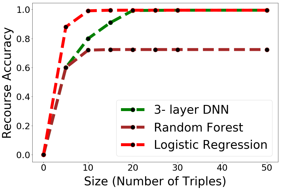
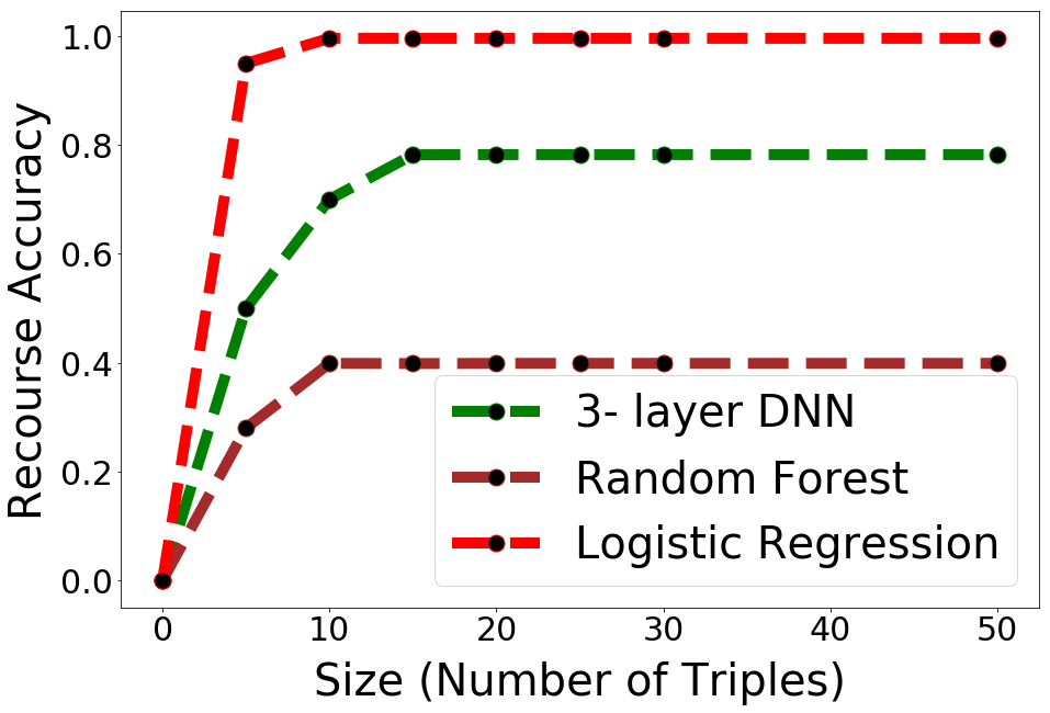
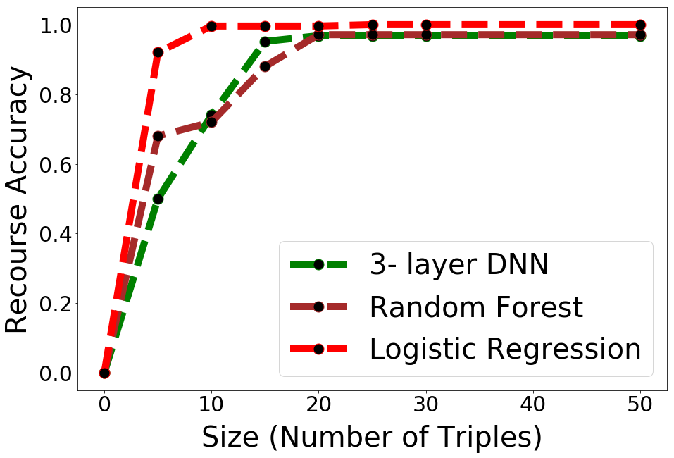
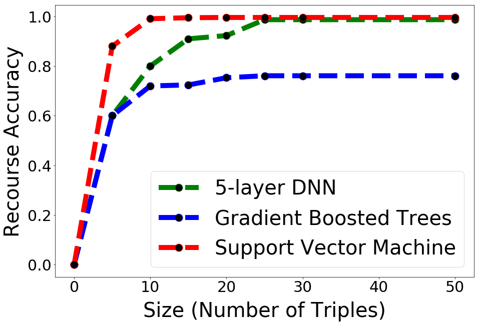
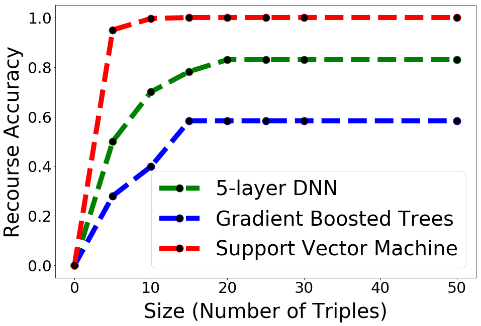
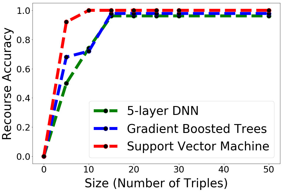
Analyzing the Trade-Offs Between Interpretability and Recourse Accuracy: Since our framework optimizes both for recourse correctness and interpretability simultaneously, it is important to understand the trade-offs between these two aspects in the context of our framework. Note that this analysis is not applicable to any other prior work on recourse generation because previously proposed approaches solely focus on generating instance-level recourses and not global summaries, and thereby do not have to account for these tradeoffs. Here, we evaluate how the recourse accuracy metric (defined above) changes as we vary the size of the two level recourse set i.e., number of triples of the form in the two level recourse set (Section 2.2). Results for the same are shown in Figure 3. It can be seen that recourse accuracies converge to their maximum values at explanation sizes of about 10 to 15 rules across all the datasets. Since humans are capable of understanding and reasoning with rule sets of this magnitude [16], results in Figure 3 establish that we are not sacrificing recourse accuracy to achieve interpretability in case of the datasets or the black box models that we are using.
Detecting Biases in Recourses - A User Study: To evaluate if users are able to detect model biases or discrimination against specific subgroups using the recourse summaries output by our framework, we carried out an online user study with 21 participants. To this end, we first constructed as our black box model a two level recourse set that was biased against one racial subgroup i.e., it required individuals of one race to change twice the number of features to obtain a desired prediction (details in Appendix). We then used our framework AReS and AR-LIME (see Baselines) to construct the recourses corresponding to this black box. Note that while our method outputs global summaries of recourses, AR-LIME can only provide instance level recourses. However, since there is no prior work which provides global summaries of recourses like we do, we use AR-LIME and average its instance level recourses as discussed in Ustun et al. [36] and use it as a comparison point for this study. Participants were randomly assigned to see either the recourses output by our method (customized to show recourses for various racial subgroups) or AR-LIME. We also provided participants with a short tutorial on recourses as well as the corresponding methods they were assigned to. Participants were then asked two questions: 1) Based on the recourses shown above, do you think the underlying black box is biased against a particular racial subgroup? 2) If so, please describe the nature of the bias in plain English.. While the first question was a multiple choice question with three answer options: yes, no, hard to determine, the second question was a descriptive one.
We then evaluated the responses of all the 21 participants. Each descriptive answer was examined by two independent evaluators and tagged as right or wrong based on if the participant’s answer accurately described the bias or not. We excluded from our analysis one response on which the evaluators did not agree. Our results show that 90% of the participants who were assigned to our method AReS were able to accurately detect that there is an underlying bias. Furthermore, 70% of these participants also described the nature of the bias accurately. On the other hand, out of the 10 participants assigned to AR-LIME, only two users (20%) were able to detect that there is an underlying bias and no user (0%) was able to describe the bias correctly. In fact, 80% of the participants assigned to AR-LIME said it was hard to determine if there is an underlying bias. These results clearly demonstrate the necessity and significance of methods which can provide accurate summaries of recourses as opposed to just individual recourses.
In addition to the above, we also experimented with introducing racial biases into a 3-layer neural network and a logistic regression model via trial and error. We then carried out similar user studies (as above) with 36 additional participants to evaluate how our explanations compared with aggregates of individual recourses. In case of the 3-layer neural network, AReS clearly outperformed AR-LIME – 88.9% vs. 44.4% on bias detection and 55.6% vs. 11.1% on bias description. In case of the logistic regression model, AReS and AR-LIME performed comparably – 88.9% in both cases on bias detection and 66.7% vs. 44.4% on bias description.
4 Conclusions
In this paper, we propose AReS, the first ever framework designed to learn global counterfactual explanations which can provide interpretable and accurate summaries of cost-effective recourses for the entire population with emphasis on specific subgroups of interest. Extensive experimentation with real world data from credit scoring and criminal justice domains as well as user studies suggest that our framework outputs interpretable and accurate summaries of recourses which can be readily used by decision makers and stakeholders to diagnose model biases and discrimination. This work paves way for several interesting future directions. First, the notions of recourse correctness, costs, and interpretability that we outline in this work can be further enriched. Our optimization framework can readily incorporate any newer notions as long as they satisfy the properties of non-negativity and submodularity. Second, it would be interesting to explore other real-world settings to which this work can be applied.
5 Broader Impact
Our framework, AReS, can be used by decision makers that wish to analyse machine learning systems for biases in recourse before deploying them in the real world. It can be applicable to a variety of domains where algorithms are making decisions and recourses are necessary–e.g., healthcare, education, insurance, credit-scoring, recruitment, and criminal justice. AReS enables the auditing of systems for fairness, and its customizable nature allows decision makers to specifically test and understand their models in a context dependent manner.
It is important to be cognizant of the fact that just like any other recourse generation algorithm, AReS may also be prone to errors. For instance, spurious recourses may be reported either due to particular configurations of hyperparameters (e.g., valuing coverage or interpretability way more than correctness) or due to the approximation algorithms we use for optimization. Such errors may translate into masking existing biases of a classifier, especially on subgroups that are particularly underrepresented in the data. It may also lead to AReS reporting nonexistent biases. It is thus important to be cognizant of the fact that AReS is finally an explainable algorithm (as opposed to being a fairness technique) that is meant to guide decision makers. It can be used to gauge the need for deeper analysis, and test for specific, known red-flags, rather than to provide concrete evidence of violations of fairness criteria.
Good use of AReS requires decision makers to be cognizant of these strengths and weaknesses. For a more complete understanding of a black box classifier before deployment, we recommend that AReS be run multiple times, with different hyperparameters and candidate sets and . Furthermore, evaluating the interpretability-recourse accuracy tradeoffs (Figure 3) can help detect any undesirable scenarios which might result in spurious recourses. Possible violations of fairness criteria discovered by AReS should be investigated further before any action is taken. Finally, we propose that when showing summaries output by AReS, the recourse accuracies of each of the recourse rules should also be included so that decision makers can make informed choices.
Acknowledgements
We would like to thank Julius Adebayo, Winston Luo, Hayoun Oh, Sarah Tan, and Berk Ustun for insightful discussions. This work is supported in part by Google. The views expressed are those of the authors and do not reflect the official policy or position of the funding agencies.
References
- [1] Rakesh Agrawal, Ramakrishnan Srikant, et al. Fast algorithms for mining association rules.
- Barocas et al. [2020] Solon Barocas, Andrew D. Selbst, and Manish Raghavan. The hidden assumptions behind counterfactual explanations and principal reasons. In Proceedings of the 2020 Conference on Fairness, Accountability, and Transparency, FAT* ’20, page 80–89, New York, NY, USA, 2020. Association for Computing Machinery. ISBN 9781450369367. doi: 10.1145/3351095.3372830. URL https://doi.org/10.1145/3351095.3372830.
- Bastani et al. [2017] Osbert Bastani, Carolyn Kim, and Hamsa Bastani. Interpretability via model extraction. arXiv preprint arXiv:1706.09773, 2017.
- Bradley and Terry [1952] Ralph Allan Bradley and Milton E. Terry. Rank analysis of incomplete block designs: I. the method of paired comparisons. Biometrika, 39(3/4):324–345, 1952. ISSN 00063444. URL http://www.jstor.org/stable/2334029.
- Caron and Doucet [2012] François Caron and Arnaud Doucet. Efficient bayesian inference for generalized bradley—terry models. Journal of Computational and Graphical Statistics, 21(1):174–196, 2012. ISSN 10618600. URL http://www.jstor.org/stable/23248829.
- Chaganty and Liang [2016] Arun Tejasvi Chaganty and Percy Liang. How much is 131 million dollars? putting numbers in perspective with compositional descriptions. arXiv preprint arXiv:1609.00070, 2016.
- Dandl et al. [2020] Susanne Dandl, Christoph Molnar, Martin Binder, and Bernd Bischl. Multi-objective counterfactual explanations. Lecture Notes in Computer Science, page 448–469, 2020. ISSN 1611-3349. doi: 10.1007/978-3-030-58112-1_31. URL http://dx.doi.org/10.1007/978-3-030-58112-1_31.
- Doshi-Velez and Kim [2017] Finale Doshi-Velez and Been Kim. Towards a rigorous science of interpretable machine learning. arXiv preprint arXiv:1702.08608, 2017.
- Dua and Graff [2017] Dheeru Dua and Casey Graff. UCI machine learning repository, 2017. URL http://archive.ics.uci.edu/ml.
- Hunter [2004] David R. Hunter. Mm algorithms for generalized bradley-terry models. Ann. Statist., 32(1):384–406, 02 2004. doi: 10.1214/aos/1079120141. URL https://doi.org/10.1214/aos/1079120141.
- Joshi et al. [2019] Shalmali Joshi, Oluwasanmi Koyejo, Warut Vijitbenjaronk, Been Kim, and Joydeep Ghosh. Towards realistic individual recourse and actionable explanations in black-box decision making systems, 2019.
- Karimi et al. [2019] Amir-Hossein Karimi, Gilles Barthe, Borja Balle, and Isabel Valera. Model-agnostic counterfactual explanations for consequential decisions, 2019.
- Karimi et al. [2020] Amir-Hossein Karimi, Bernhard Schölkopf, and Isabel Valera. Algorithmic recourse: from counterfactual explanations to interventions, 2020.
- Khuller et al. [1999] Samir Khuller, Anna Moss, and Joseph Seffi Naor. The budgeted maximum coverage problem. Information Processing Letters, 70(1):39–45, 1999.
- Koh and Liang [2017] Pang Wei Koh and Percy Liang. Understanding black-box predictions via influence functions. In Proceedings of the 34th International Conference on Machine Learning-Volume 70, pages 1885–1894. JMLR. org, 2017.
- Lakkaraju et al. [2016] Himabindu Lakkaraju, Stephen H Bach, and Jure Leskovec. Interpretable decision sets: A joint framework for description and prediction. In Proceedings of the 22nd ACM SIGKDD international conference on knowledge discovery and data mining, pages 1675–1684, 2016.
- Lakkaraju et al. [2019] Himabindu Lakkaraju, Ece Kamar, Rich Caruana, and Jure Leskovec. Faithful and customizable explanations of black box models. In Proceedings of the 2019 AAAI/ACM Conference on AI, Ethics, and Society, pages 131–138. ACM, 2019.
- Larson et al. [2016] Jeff Larson, Surya Mattu, Lauren Kirchner, and Julia Angwin. How we analyzed the compas recidivism algorithm, May 2016. URL https://www.propublica.org/article/how-we-analyzed-the-compas-recidivism-algorithm.
- Lee et al. [2009] Jon Lee, Vahab S Mirrokni, Viswanath Nagarajan, and Maxim Sviridenko. Non-monotone submodular maximization under matroid and knapsack constraints. In Proceedings of the forty-first annual ACM symposium on Theory of computing, pages 323–332. ACM, 2009.
- Looveren and Klaise [2019] Arnaud Van Looveren and Janis Klaise. Interpretable counterfactual explanations guided by prototypes, 2019.
- Luce [1959] R.D. Luce. Individual choice behavior: a theoretical analysis. Wiley, 1959. URL https://books.google.com/books?id=a80DAQAAIAAJ.
- Lucic et al. [2019] Ana Lucic, Harrie Oosterhuis, Hinda Haned, and Maarten de Rijke. Actionable interpretability through optimizable counterfactual explanations for tree ensembles, 2019.
- Lundberg and Lee [2017] Scott M Lundberg and Su-In Lee. A unified approach to interpreting model predictions. In Advances in Neural Information Processing Systems, pages 4765–4774, 2017.
- Mothilal et al. [2020] Ramaravind K. Mothilal, Amit Sharma, and Chenhao Tan. Explaining machine learning classifiers through diverse counterfactual explanations. Proceedings of the 2020 Conference on Fairness, Accountability, and Transparency, Jan 2020. doi: 10.1145/3351095.3372850. URL http://dx.doi.org/10.1145/3351095.3372850.
- Pawelczyk et al. [2020] Martin Pawelczyk, Klaus Broelemann, and Gjergji Kasneci. Learning model-agnostic counterfactual explanations for tabular data. Proceedings of The Web Conference 2020, Apr 2020. doi: 10.1145/3366423.3380087. URL http://dx.doi.org/10.1145/3366423.3380087.
- Plumb et al. [2020] Gregory Plumb, Jonathan Terhorst, Sriram Sankararaman, and Ameet Talwalkar. Explaining groups of points in low-dimensional representations, 2020.
- Poyiadzi et al. [2020] Rafael Poyiadzi, Kacper Sokol, Raul Santos-Rodriguez, Tijl De Bie, and Peter Flach. Face: Feasible and actionable counterfactual explanations. In Proceedings of the AAAI/ACM Conference on AI, Ethics, and Society, AIES ’20, page 344–350, New York, NY, USA, 2020. Association for Computing Machinery. ISBN 9781450371100. doi: 10.1145/3375627.3375850. URL https://doi.org/10.1145/3375627.3375850.
- Rathi [2019] Shubham Rathi. Generating counterfactual and contrastive explanations using shap, 2019.
- Ribeiro et al. [2016] Marco Tulio Ribeiro, Sameer Singh, and Carlos Guestrin. " why should i trust you?" explaining the predictions of any classifier. In Proceedings of the 22nd ACM SIGKDD international conference on knowledge discovery and data mining, pages 1135–1144, 2016.
- Ribeiro et al. [2018] Marco Tulio Ribeiro, Sameer Singh, and Carlos Guestrin. Anchors: High-precision model-agnostic explanations. In Thirty-Second AAAI Conference on Artificial Intelligence, 2018.
- Selvaraju et al. [2017] Ramprasaath R Selvaraju, Michael Cogswell, Abhishek Das, Ramakrishna Vedantam, Devi Parikh, and Dhruv Batra. Grad-cam: Visual explanations from deep networks via gradient-based localization. In Proceedings of the IEEE international conference on computer vision, pages 618–626, 2017.
- Simonyan et al. [2013] Karen Simonyan, Andrea Vedaldi, and Andrew Zisserman. Deep inside convolutional networks: Visualising image classification models and saliency maps. arXiv preprint arXiv:1312.6034, 2013.
- Smilkov et al. [2017] Daniel Smilkov, Nikhil Thorat, Been Kim, Fernanda Viégas, and Martin Wattenberg. Smoothgrad: removing noise by adding noise. arXiv preprint arXiv:1706.03825, 2017.
- Sundararajan et al. [2017] Mukund Sundararajan, Ankur Taly, and Qiqi Yan. Axiomatic attribution for deep networks. In Proceedings of the 34th International Conference on Machine Learning-Volume 70, pages 3319–3328. JMLR. org, 2017.
- Tolomei et al. [2017] Gabriele Tolomei, Fabrizio Silvestri, Andrew Haines, and Mounia Lalmas. Interpretable predictions of tree-based ensembles via actionable feature tweaking. Proceedings of the 23rd ACM SIGKDD International Conference on Knowledge Discovery and Data Mining, Aug 2017. doi: 10.1145/3097983.3098039. URL http://dx.doi.org/10.1145/3097983.3098039.
- Ustun et al. [2019] Berk Ustun, Alexander Spangher, and Yang Liu. Actionable recourse in linear classification. Proceedings of the Conference on Fairness, Accountability, and Transparency - FAT* ’19, 2019. doi: 10.1145/3287560.3287566. URL http://dx.doi.org/10.1145/3287560.3287566.
- Venkatasubramanian and Alfano [2020] Suresh Venkatasubramanian and Mark Alfano. The philosophical basis of algorithmic recourse. In Proceedings of the 2020 Conference on Fairness, Accountability, and Transparency, FAT* ’20, page 284–293, New York, NY, USA, 2020. Association for Computing Machinery. ISBN 9781450369367. doi: 10.1145/3351095.3372876. URL https://doi.org/10.1145/3351095.3372876.
- [38] Paul Voigt and Axel Von dem Bussche. The eu general data protection regulation (gdpr).
- Wachter et al. [2018] S Wachter, BDM Mittelstadt, and C Russell. Counterfactual explanations without opening the black box: automated decisions and the gdpr. Harvard Journal of Law and Technology, 31(2):841–887, 2018.
Appendix A Appendix
A.1 Proofs for Theorems
Theorem 2.1. The objective function in Equation 1 is non-normal, non-negative, non-monotone, submodular, and the constraints of the optimization problem are matroids.
Proof.
In order to prove that the objective function in Eqn. 1 is non-normal, non-negative, non-monotone, and submodular, we need to prove the following:
-
•
any one of the terms in the objective is non-normal
-
•
all the terms in the objective are non-negative
-
•
any one of the terms in the objective is non-monotone
-
•
all the terms in the objective are submodular
Non-normality
Let us consider the term . If is normal, then .
It can be seen from the definition of that because incorrectrecourse by definition. This also implies that . Therefore is non-normal and consequently the entire objective is non-normal.
Non-negativity
The functions are non-negative because first term in each of these is an upper bound on the second term. Therefore, each of these will always have a value . In the case of which encapsulates the cover metric which is the number of instances which satisfy some recourse rule in the explanation. This metric can never be negative by definition. Since all the functions are non-negative, the objective itself is non-negative.
Non-monotonicity
Let us choose the term . Let us consider two explanations (two level recourse sets) and such that . If is monotonic then, . Let us see if this condition holds:
Based on the definition of incorrectrecourse metric, it is easy to note that
This is because has at least as many rules as that of . This implies the following:
This shows that is non-monotone and therefore the entire objective is non-monotone.
Submodularity
Let us go over each of the terms in the objective and show that each one of those is submodular.
Let us consider two explanations (two level recourse sets) and such that . A function is considered to be submodular if where .
By definition of incorrectrecourse, each time a triple is added to some explanation , the value of incorrectrecourse is simply incremented by the number of data points for which this triple assigns recourse incorrectly. This implies that this metric is modular which in turn means is also modular and thereby submodular i.e.,
is the cover metric which denotes the number of instances that satisfy some rule in the explanation. This is clearly a diminishing returns function i.e., more additional instances in the data are covered when we add a new rule to a smaller two level recourse set compared to a larger one. Therefore, is submodular.
featurecost and featurechange are both additive in that each time a triple is added to some explanation , the value of these metrics is incremented either by the sum of costs of corresponding features which need to be changed (featurecost) or the sum of changes in magnitudes of the features (featurechange). This implies that these metrics are modular which in turn means and are modular and thereby submodular.
Constraints: A constraint is a matroid if it has the following properties: 1) satisfies the constraint 2) if 2 two level recourse sets and satisfy the constraint and , then adding an element s.t. , to should result in a set that also satisfies the constraint. It can be seen that these two conditions hold for all our constraints. For instance, if a two level recourse set has rules (i.e., size() ) and another two level recourse set has fewer rules than , then the set resulting from adding any element of to the smaller set will still satisfy the constraint on size. Similarly, the constraints on maxwidth and numrsets satisfy the aforementioned properties too. ∎
Before we prove Theorem 2.2, we will first discuss how several previously proposed methods which provide recourses for affected individuals (i.e., instance level recourses) can be unified into one basic algorithm.
Unifying Prior Work
The algorithm below unifies multiple prior instance-level recourse finding techniques namely Wachter et al. [39], Ustun et al. [36], Karimi et al. [12]. All the aforementioned techniques employ a generalized optimization procedure that searches for a minimum cost recourse for every affected individual by constantly polling the classifier with different candidate recourses until a valid recourse is found [7]. The search for valid recourses is guided by the function, which generates candidates with progressively higher costs (with the definition of cost varying by technique). For example, Wachter et al. [39] use ADAM to optimize their cost function, - where represents a distance metric (e.g., L1 norm), to repeatedly generate candidates for increasingly farther away from , until one of them finally flips the classifier prediction. Similarly, Karimi et al. [12] use boolean SAT solvers to exhaustively generate candidate modifications , while Ustun et al. [36] use integer programming to generate candidate modifications that are monotonically non-decreasing in cost, thus providing the theoretical guarantee of finding minimum cost recourse for linear models.
Theorem 2.2 If all features take on values from a finite set, then the optimization problem in Eqn.1 can be reduced to the objectives employed by prior approaches which provide instance level counterfactuals for individual recourse.
Proof.
To prove this theorem, we will first describe how instance level counterfactuals for indivual recourses can be generated using our framework AReS. Then, we show how this is equivalent to the objectives outlined in Wachter et al. [39], Ustun et al. [36], Karimi et al. [12].
Generating instance level counterfactuals for individual recourses using AReS: If a conjunction consists of the entire feature-vector of a particular data-point , then the triple represents a single instance level counterfactual. This is how AReS can be used to output individual recourses.
Subsuming other objective functions: The objective optimized by Wachter et al. is . This can be equivalently expressed in our notation from Table 1 as , where the first term captures how closely the prediction resulting from the prescribed recourse matches the desired prediction, and the second term represents the distance between the counterfactual and the original data point . The aforementioned two expressions are equivalent because our setting consists only of binary classifiers with outputs. In this case, our definition of incorrectrecourse is identical to incorrectrecourse. Similarly, from our notation is the same as . As described in algorithm 1, all recourse search techniques use the notion captured by and some form of distance metric or cost function, captured by or the customizable in AReS.
Let the (finite) set of all possible feature vectors be denoted by . Note that , and setting in AReS would allow the recourse search to be over the entire domain of the data. Setting size and further mandates that the final recourse set consists of only one triple , which contains the recourse desired for the feature-vector . Further, since most instance level recourse generation techniques do not have additional interpretability constraints [39, 36, 27, 12, 20, 25] such as the and terms in AReS, we set . Finally, setting leaves us with as our objective function, which represents the exact same optimization as that of Wachter et al. [39]. Similar configurations (e.g. setting instead of , and defining cost of each feature in terms of percentile shift in feature values) will yield the objective functions used by other recourse generation techniques (e.g. Ustun et al.’s Actionable Recourse). ∎
Theorem 2.3 If the underlying model provides recourse to all individuals, then upper bound on the proportion of individuals in for whom AReS outputs an incorrect recourse is , where is the approximation ratio of the algorithm used to optimize Eqn 1.
Proof.
Let represent the maximum possible value of the objective function defined in Eqn. 1. Let represent the objective value for the two level recourse set which provides correct recourse to a single arbitrary data point (i.e., ) which is obtained by setting and . Therefore, and due to the approximation ratio () of the algorithm used to optimize Eqn. 1.
| (2) | ||||
| (3) | ||||
| subtracting (3) from (2), we get | ||||
| (4) | ||||
Optimizing only for recourse correctness of a single arbitrary instance i.e., setting and , we have . Therefore, Eqn. (4) can be written as:
∎
This establishes that the upper bound on the proportion of individuals in for whom AReS outputs an incorrect recourse is .
A.2 Experimental Evaluation
A.2.1 Parameter Tuning
We set the parameters as follows. First, we set aside 5% of the dataset as a validation set to tune these parameters. We first initialize the value of each to . We then carry out a coordinate descent style approach where we decrement the values of each of these parameters while keeping others constant until one of the following conditions is violated: 1) less than 95% of the instances in the validation set are covered by the resulting explanation 2) more than 2% of the instances in the validation set are covered by multiple rules in the explanation 3) the prescribed recourses result in incorrect labels for more than 15% of the instances (for whom the black box assigned label ) in the validation set.
| Algorithms | Datasets | ||||||
| COMPAS | Credit | Bail | |||||
| Recourse | Mean | Recourse | Mean | Recourse | Mean | ||
| Accuracy | FCost | Accuracy | Fcost | Accuracy | Fcost | ||
| DNN-5 | AR-LIME | 99.67% | 2.93 | 0% | NA | 84.49% | 2.59 |
| AR-KMeans | 65.89% | 6.07 | 47.06% | 1.68 | 92.25% | 7.31 | |
| FACE | 88.28% | 5.43 | 68.31% | 2.25 | 83.31% | 5.64 | |
| AReS | 98.72% | 1.92 | 83.02% | 1.03 | 96.18% | 1.88 | |
| GBT | AR-LIME | 21.57% | 5.21 | 8.00% | 3.44 | 69.17% | 2.40 |
| AR-KMeans | 60.08% | 5.34 | 22.33% | 3.40 | 93.03% | 7.14 | |
| FACE | 55.87% | 5.42 | 24.38% | 3.41 | 77.82% | 5.63 | |
| AReS | 76.17% | 3.88 | 58.32% | 1.67 | 97.84% | 1.18 | |
| SVM | AR | 100% | 1.25 | 100% | 7.84 | 100% | 7.93 |
| FACE | 95.63% | 1.43 | 93.10% | 5.77 | 88.12% | 7.02 | |
| AReS | 99.64 | 0.88 | 100% | 2.45 | 100% | 4.35 | |
A.2.2 User Study
We manually constructed a two level recourse set (as our black box model) for the bail application. We deliberately ensured that this black box was biased against individuals who are not Caucasian. More specifically, we induced the following bias: individuals who are not Caucasian are required to change twice the number of features to obtain a desired prediction compared to those who are Caucasian. This two level recourse set (black box) is shown in Figure 4.
We then used our approach and 95% of the bail dataset to learn a two level recourse set explanation (remaining 5% of the data is used for tuning parameters). We also set all feature costs to . We found that our approach was able to exactly recover the underlying model and thereby obtain a recourse accuracy of 100%. We used AR-LIME as a comparison point in our user study. Note that while our method outputs global summaries of recourses, AR-LIME can only provide instance level recourses. However, since there is no prior work which provides global summaries of recourses like we do, we use AR-LIME and average its instance level recourses as discussed in Ustun et al. [36]. More specifically, we first run AR-LIME to obtain individual recourses and then for each possible subgroup of interest, we will average the recourses over all individuals within that subgroup (as suggested in Ustun et al. [36]). We found that such an averaging was actually resulting in incorrect summaries which are misleading. This in turn reflected in the user responses of our user study.
| If Race Caucasian: |
| If Married No and Property No and Has Job No, then Married No and Property No and Has Job Yes |
| If Drugs Yes and School No and Pays Rent No , then Drugs No and School No and Pays Rent No |
| If Race Caucasian: |
| If Married No and Property No and Has Job No, then Married No and Property Yes and Has Job Yes |
| If Drugs Yes and School No and Pays Rent No , then Drugs No and School No and Pays Rent Yes |
| If Female No and Foreign Worker No: |
| If Missed Payments Yes and Critical Loans Yes, then Missed Payments Yes and Critical Loans No |
| If Unemployed Yes and Critical Loans Yes and Has Guarantor No, |
| then Unemployed Yes and Critical Loans No and Has Guarantor Yes |
| If Female No and Foreign Worker Yes: |
| If Skilled Job No and Years at Job 1, then Skilled Job Yes and Years at Job 4 |
| If Unemployed Yes and Has Guarantor No and Has CoAppplicant No, |
| then Unemployed No and Has Guarantor Yes and Has CoAppplicant Yes |
| If Female Yes: |
| If Married No and Owns House No, then Married Yes and Owns House Yes |
| If Unemployed No and Has Guarantor Yes and Has CoAppplicant No, |
| then Unemployed No and Has Guarantor Yes and Has CoAppplicant Yes |