Stable two-dimensional soliton complexes in Bose-Einstein condensates with helicoidal spin-orbit coupling

Abstract

We show that attractive two-dimensional spinor Bose-Einstein condensates with helicoidal spatially periodic spin-orbit coupling (SOC) support a rich variety of stable fundamental solitons and bound soliton complexes. Such states exist with chemical potentials belonging to the semi-infinite gap in the band spectrum created by the periodically modulated SOC. All these states exist above a certain threshold value of the norm. The chemical potential of fundamental solitons attains the bottom of the lowest band, whose locus is a ring in the space of Bloch momenta, and the radius of the ring is a non-monotonous function of the SOC strength. The chemical potential of soliton complexes does not attain the band edge. The complexes are bound states of several out-of-phase fundamental solitons whose centers are placed at local maxima of the SOC-modulation phase. In this sense, the impact of the helicoidal SOC landscape on the solitons is similar to that of a periodic two-dimensional potential. In particular, it can compensate repulsive forces between out-of-phase solitons, making their bound states stable. Extended stability domains are found for complexes built of two and four solitons (dipoles and quadrupoles, respectively). They are typically stable below a critical value of the chemical potential.

Keywords: Solitons; matter waves, spin-orbit coupling, quantum gases

1 Introduction

Spin-orbit coupling (SOC) is a fundamentally important effect in physics of semiconductors, whose theoretical models [1, 2] and experimental manifestations [3, 4] have been known for a long time. More recently, much interest was drawn to emulation of SOC in binary ultracold gases [chiefly, these are two-component Bose-Einstein condensates (BEC)] [5, 6, 7, 8]. The SOC emulation proceeds by mapping the spinor wave function of electrons in semiconductors into a pseudo-spinor mean-field wave function in BEC, whose components represent two atomic states in the condensate. Although, in this way, fermionic spinors are emulated by a pair of hyperfine states of bosonic atoms, the basic SOC Hamiltonians of the Dresselhaus [1] and Rashba [2] types, equivalent to non-Abelian or Abelian (depending on the realization) spin-related gauge fields, can be efficiently reproduced in BECs illuminated by properly designed sets of laser beams.

While SOC in bosonic gases is a linear effect, its interplay with the intrinsic BEC nonlinearity, induced by interatomic interactions, was predicted to give rise to various species of self-trapped mean-field states [9], including several types of one-dimensional (1D) solitons [10, 11, 12, 13, 14, 15, 16]. Experimental realization of SOC in an effectively two-dimensional (2D) geometry was reported too [17], which suggests to consider, in particular, a possibility of the creation of 2D gap solitons, supported by a combination of SOC and a spatially periodic field induced by an optical lattice (OL) [18].

A fundamental problem which impedes the creation of 2D and 3D solitons in BEC, nonlinear optics, and other nonlinear settings, is that the ubiquitous cubic self-attraction, which usually gives rise to solitons, simultaneously drives the critical and supercritical collapse (catastrophic self-compression) in the 2D and 3D cases, respectively [19, 20]. Although SOC modifies the conditions of the existence of solutions and of the blow up, it does not arrest the collapse completely [21]. The collapse destabilizes formally existing solitons, which makes stabilization of 2D and 3D solitons a well-known challenging problem [22, 23]. In particular, it is well known that OL-induced potentials provide a universal method for the creation of stable multidimensional solitons, including those with embedded vorticity (topological charge) [24, 25, 26]. In the absence of OL potentials, the cubic self-attraction makes vortex solitons extremely unstable modes [27, 28].

An essential fact, first revealed in Ref. [29], is that the standard SOC of the Rashba type, added to the usual two-component system of Gross-Pitaevskii equations (GPEs) with the attractive cubic interactions [of both self- and cross-phase-modulation (SPM and XPM) types, i.e., self- and cross-interactions, respectively], readily supports stable solitons of two types: semivortices, SVs (with one zero-vorticity component and the other one with vorticity $1$), and mixed modes, MMs (with vorticities $-1,0$, and $1$ blended in both components). Formation of stable states involving nonzero vorticity can be seen as a result of a counterflow produced by anomalous spin-dependent velocity determined by SOC [30]. These SVs and MMs are stable, severally, in the system with XPM stronger than SPM, and vice versa. Both SV and MM species are stable in the case of equal strengths of the SPM and XPM terms (the Manakov’s nonlinearity [31]). When the SV or MM is stable, it represents the system’s ground state (in the absence of SOC, the ground state is missing in the unstable BEC), provided that the total norm of the pseudo-spinor wave function does not exceed a critical value (in fact, it is the norm of the Townes soliton [32], which is an unstable solution of GPE in 2D in the absence of SOC [19, 20]). Above the critical norm, where the centrifugal counterflow, induced by the anomalous velocity [30], cannot overcome the attraction-induced density flux, the collapse still takes place, albeit being modified by the SOC. In [18] it was shown that SOC stabilizes solitons, gap-solitons and half-vortices of different symmetries in Zeeman lattices. Later, similar results for stable 2D solitons of the SV and MM types were reported for the SOC of a more general type, combining the Rashba and Dresselhaus couplings [33], as well as for the binary BEC of ”heavy atoms”, for which the kinetic energy (second derivatives in GPE) may be neglected in comparison with the SOC energy, represented by first-order cross-derivatives in the GPE system [34]. Also demonstrated [35] were the stabilizations of MM states by SOC in a system including additional nonlinearity which represents the beyond-mean-field corrections of the Lee-Huang-Yang type [36, 37, 38, 39, 40, 41, 42]. Eventually, the creation of metastable solitons of both SV and MM types was predicted in the 3D system with SOC [43]. Furthermore, it was demonstrated that the SOC with reduced dimensionality, viz., one- or two-dimensional Rashba coupling acting in the 2D or 3D space, is sufficient for the stabilization of the 2D and 3D solitons, respectively [44]. The SOC acting in a spatially confined area is also sufficient for maintaining stable 1D [14] and 2D [45] solitons.

More generally, the stabilizing effect of gauge fields is known even since earlier times. In [46] it was shown that stable solitons in one-component 2D BECs can be sustained by the rotating trap emulating a gauge field. Confinement of a spinor BEC in the quasi-relativistic limit by a gauge field was reported in [47]. Recently, in [48] it was discovered that field components, taken in a pure or non-pure gauge form, affect the soliton dynamics in very different ways. Localization characteristics of nonlinear states are determined by the curvature originating from the non-pure gauge field, while the pure gauge field strongly affects the stability of the modes. The respective solutions represent envelopes formed by a non-pure gauge field, which modulates stationary carrier states created by a pure gauge field. In coupled 1D nonlinear Schrödinger equations with SU(2)-invariant nonlinearity, a non-uniform pure gauge field preserves the integrability of the system [16]. The total effect of a SOC gauge field can lead not only to the enhanced stability of solitons in media with attractive interactions, but also to the existence of novel stable localized modes – quasisolitons – in purely repulsive condensates, both in the free space and in the presence of traps [48].

In addition to the BEC realm, SOC may be emulated in terms of nonlinear optics. In that connection, stabilization of 2D spatiotemporal optical solitons in a dual-core planar waveguide with the help of the counterpart of the BEC effect, which is represented by temporal dispersion of the inter-core coupling, was predicted in Ref. [49].

Although SOC appears to be a universal mechanism for the stabilization of 2D solitons, its efficiency is limited. It cannot stabilize excited states, obtained by adding equal vorticities to both components of SV and MM solitons in attractive media [29], although stable quasisolitons with embedded vorticity in both components in media with repulsive cubic interactions have been found [48]. Possibilities of maintaining bound states of separated solitons by SOC are not yet known either. For this reason, a relevant possibility, which we pursue in this work, is to consider SOC in the 2D geometry, subject to spatially periodic modulation (solitons and their interactions in a 1D BEC with a helicoidal SOC were considered in [15]). In the experiment, this setting can be implemented by means of an appropriate OL, which determines the spatially periodic SOC structure. As we demonstrate below, this system, with a helicoidal orientation of the local SOC [see equation (1)], gives rise to a vast stability region for fundamental 2D pseudo-spinor solitons. Further, it also produces stable dipole and quadrupole bound states of fundamental solitons with opposite signs, which cannot be found in the absence of the spatially-periodic modulation. We also demonstrate that stable solitons form sets of states, generated from a seed one by symmetry transformations.

The rest of the paper is organized as follows. The pseudo-spin system of coupled GPEs is formulated in Section 2, where we also produce its linear spectrum, in the numerical form in the general case, and analytically in the long-wave limit. Symmetries of the system are considered in Section 3. Systematic numerical results for fundamental solitons, dipoles, and quadrupoles, including the analysis of their stability and symmetry, are presented in Section 4. The paper is concluded by Section 5.

2 The model and linear spectrum of the system

We describe the evolution of the 2D spinor BEC in the presence of SOC by coupled GPEs for a spinor wave function ${\bm{\Psi}}=(\Psi_{1},\Psi_{2})^{\mathrm{T}}$:

$$i\partial_{t}{\bm{\Psi}}=\frac{1}{2}[(-i\sigma_{0}\partial_{x}+\alpha({\bm{\sigma}}{\bm{n}}))^{2}+(-i\sigma_{0}\partial_{y}+\alpha({\bm{\sigma}}{\bm{m}}))^{2}]{\bm{\Psi}}-({\bm{\Psi}}^{{\dagger}}{\bm{\Psi}}){\bm{\Psi}}.$$ (1)

Here ${\bm{\sigma}}=(\sigma_{1},\sigma_{2},\sigma_{3})$ is the vector of the Pauli matrices, $\sigma_{0}$ is the identity matrix, $\alpha$ is the strength of SOC and the position-dependent unit vectors ${\bm{n}}$ and ${\bm{m}}$ determine the SOC direction. We consider a helicoidal SOC with ${\bm{n}}=(\cos\theta(x,y),0,\sin\theta(x,y))$ and ${\bm{m}}=(-\sin\theta(x,y),0,\cos\theta(x,y))$. The above choice of vectors ${\bm{m}}$ and ${\bm{n}}$ yields the components of a non-Abelian spin-dependent gauge field

$$A_{x}=-\alpha\left(\sigma_{1}\cos\theta+\sigma_{3}\sin\theta\right),\quad A_{y}=\alpha\left(\sigma_{1}\sin\theta-\sigma_{3}\cos\theta\right)$$ (2)

with a position-independent commutator, $[A_{x},A_{y}]=-2i\alpha^{2}\sigma_{2}.$

In what follows, we concentrate on a spin-orbit coupling realized with a lattice symmetry. In this choice the coordinate-dependent phase $\theta(x,y)$ is given by

$$\theta(x,y)=\frac{\pi}{2}[\cos(\lambda_{x}x)+\cos(\lambda_{y}y)],$$ (3)

with periods $2\pi/\lambda_{x,y}$, as shown in figure 1.

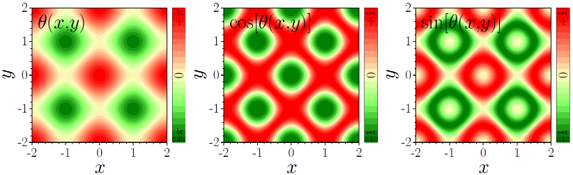
Figure 1: The left panel: contour plot of $\theta(x,y)$, drawn as per equation (3), with $\lambda_{x}=\lambda_{y}=\pi$. Middle and right panels: plots of $\cos\theta(x,y)$ and $\sin\theta(x,y),$ which determine directions of local vectors ${\bm{n}}$ and ${\bm{m}}.$

The system includes the attractive nonlinearity with equal strengths of the self- and cross-interactions in equation (1). We stress that no Zeeman splitting, which may stabilize solitons in other SOC models [15, 48], or external potential is present in equation (1). Although the stabilization of fundamental solitons in the present setting may be provided by the uniform SOC [29], it is demonstrated below that the spatially periodic modulation of local SOC is necessary to create stable multisoliton complexes (dipoles and quadrupoles), which do not exist in the uniform space.

The model (1), (3) has three length parameters. Two of them, $2\pi/\lambda_{x,y},$ are the lattice constants. The third one, $1/\alpha,$ usually referred to as the “spin-flip length” and characterizing the coordinate dependence of a spinor describing spin 1/2 particle [3] can, in general, be scaled out, i.e., the dynamics is governed by $\lambda_{x,y}/\alpha$ ratios. Nevertheless, for the analysis of different limiting cases it is convenient to keep $\alpha$ and $\lambda_{x,y}$ as separate parameters.

Before analyzing nonlinear states supported by equation (1), it is instructive to consider the spectrum of linear modes determined by Hamiltonian $H,$ which represents the kinetic energy $H_{\rm kin}$ and spin-orbit coupling $H_{\rm soc}$ in equation (1) in the form:

$$H=H_{\rm kin}+H_{\rm soc}+\alpha^{2}\sigma_{0}.$$ (4)

Here

$$H_{\rm kin}=-\frac{1}{2}\nabla^{2}\sigma_{0}$$ (5)

has the spin-diagonal form. The other contribution, $H_{\rm soc},$ can be presented as the sum of two terms:

$$H_{\rm soc}=H_{{\rm soc}|0}+H_{{\rm soc}|1},$$ (6)

defined as:

$$H_{{\rm soc}|0}=-i\alpha\left(\begin{array}[]{cc}\sin\theta&\cos\theta\\ \cos\theta&-\sin\theta\end{array}\right)\partial_{x}-i\alpha\left(\begin{array}[]{cc}\cos\theta&-\sin\theta\\ -\sin\theta&-\cos\theta\end{array}\right)\partial_{y},$$ (7)

and

$$H_{{\rm soc}|1}=-\frac{i}{2}\alpha(\partial_{x}\theta)\left(\begin{array}[]{cc}\cos\theta&-\sin\theta\\ -\sin\theta&-\cos\theta\end{array}\right)-\frac{i}{2}\alpha(\partial_{y}\theta)\left(\begin{array}[]{cc}-\sin\theta&-\cos\theta\\ -\cos\theta&\sin\theta\end{array}\right).$$ (8)

Hereafter we omitted the explicit spatial dependence where it is not required directly.

As coefficients in equation (1) are periodic functions of $x$ and $y,$ we seek for eigenfunctions in the form of Bloch waves

$${\bm{\Psi}}=\left(\begin{array}[]{c}C_{\uparrow}(x,y)\\ C_{\downarrow}(x,y)\end{array}\right)\exp\left[i\left({\bm{k}}{\bm{r}}-\mu_{\mathrm{lin}}({\bm{k}})t\right)\right],$$ (9)

where ${\bm{r}}=(x,y)$, $C_{\uparrow,\downarrow}(x,y)=C_{\uparrow,\downarrow}(x+2\pi/\lambda_{x},y)=C_{\uparrow,\downarrow}(x,y+2\pi/\lambda_{y})$ are components of a time-independent spatially-periodic spinor wave function, $k_{x,y}$ are the Bloch momenta in the first Brillouin zone, $\mu_{\mathrm{lin}}({\bm{k}})$ is the chemical potential of the linear system, and we omitted the Bloch band index since we are interested only in the lowest bands. The substitution of the Bloch ansatz (9) in the linearized version of equation (1) leads to an eigenvalue problem,

$$H\Psi=\mu_{\mathrm{lin}}({\bm{k}})\Psi,$$ (10)

which determines the bandgap spectrum of the system, $\mu_{\mathrm{lin}}({\bm{k}})$.

We begin with a particle in the free space, where we can set $\lambda_{x}=\lambda_{y}=0$ and $\theta=\pi,$ the coefficients $C_{\uparrow,\downarrow}(x,y)$ are position-independent, and the values of $k_{x,y}$ are not restricted. According to equation (10) the chemical potential in this case becomes $\mu_{\mathrm{lin}}({\bm{k}})=\alpha^{2}+k^{2}/2\pm\alpha\,k,$ where $k\equiv(k_{x}^{2}+k_{y}^{2})^{1/2}$ and the spinor components, for different values of $\mu_{\mathrm{lin}}({\bm{k}}),$ satisfy conditions

$$|C_{\uparrow}|^{2}=\frac{k\pm k_{y}}{2k},\qquad|C_{\downarrow}|^{2}=\frac{k\mp k_{y}}{2k},$$ (11)

where upper/lower sign corresponds to the sign in front of $\alpha k$ in $\mu_{\mathrm{lin}}({\bm{k}}).$

In what follows we concentrate on a square lattice with parameters $\lambda_{x}=\lambda_{y}\equiv\lambda$ and begin with displaying two numerically calculated lowest bands of the linear spectrum in figures 2(a,b). The solitons of our interest, formed by the attractive nonlinearity, belong to the semi-infinite gap with the values of $\mu$ below the bottom of the lowest band. As one can see from two cuts of the linear dispersion relation, shown in figures 2(a,b), the minimum of $\mu_{\mathrm{lin}}({\bm{k}})$ is achieved on the ring of radius $k_{\min}$ in the $(k_{x},k_{y})$ plane. The radius of this ring, being a non-monotonous function of $\alpha$, shown in figure 2(c) by the black curve, may shrink to zero at certain values of $\alpha,$ while it monotonously increases at a sufficiently strong SOC.

For small Bloch momenta, $\left|k\right|\ll\lambda$, and small SOC strength, $\alpha\ll\lambda$, one can find the spectrum in an approximate analytical form by means of averaging with respect to relatively rapid oscillations of $\cos\theta(x,y)$ and $\sin\theta(x,y)$, while keeping the slowly oscillating function $\exp\left(i{\bm{k}}{\bm{r}}\right)$ in ansatz (9). A nontrivial result can be obtained in the asymptotic regime defined by the following relation between the two small parameters: $k\sim\alpha.$ Under this condition, in the zero-order approximation the spinor wave function in equation (9) does not depend on the coordinates, $C_{\uparrow,\downarrow}^{(0)}=\mathrm{const}$, an estimate for the lowest-order corrections to it being $\delta\left(C_{\uparrow,\downarrow}\right)\sim\alpha k/\lambda^{2}.$ Then, the kinetic energy term in Hamiltonian (5) yields an obvious lowest-order contribution to the eigenvalue, that is $k^{2}/2$. In the same approximation, a contribution of terms $\sim i\alpha\partial_{x,y}$ in (6) can be found as eigenvalues of the respective matrix with entries, $\cos\theta(x,y)$ and $\sin\theta(x,y)$, replaced by their spatially average values, $\left\langle\cos\theta(x,y)\right\rangle\equiv\mathrm{{\mathcal{C}}}$ and $\left\langle\sin\theta(x,y)\right\rangle\equiv\mathrm{{\mathcal{S}}}$, and $-i\partial_{x,y}$ replaced by $k_{x,y}$, the result being $\pm\alpha\sqrt{\mathrm{{\mathcal{C}}}^{2}+\mathrm{{\mathcal{S}}}^{2}}k$. As concerns corrections to the eigenvalues produced by corrections to the eigenfunctions given by this $\delta\left(C_{\uparrow,\downarrow}\right)$, they scale as $\delta\mu\sim\left(\alpha k\right)^{2}$, being negligible in comparison with the terms written above. In fact, the current approximation is similar to the lowest-order perturbation theory in quantum mechanics, which produces the first contribution to the eigenvalue of energy, induced by a perturbation Hamiltonian, omitting a correction to the stationary wave function.

Thus, collecting the above terms, the lowest-order approximation for the spectrum at small $k$ and $\alpha$ is obtained as

$$\mu_{\mathrm{lin}}({\bm{k}})-\mu_{\mathrm{lin}}(0)=\frac{k^{2}}{2}\pm\alpha\sqrt{\mathrm{{\mathcal{C}}}^{2}+\mathrm{{\mathcal{S}}}^{2}}k.$$ (12)

This result is written with respect to $\mu_{\mathrm{lin}}(0)$ because the calculation of $\mu_{\mathrm{lin}}(0)$ is more cumbersome, as the contribution to it from the last two terms in Hamiltonian (4) requires a calculation of the first correction to the spinor eigenfunction, the result being $\mu_{\mathrm{lin}}(0)=\alpha^{2}\left(1+{\mathcal{C}}^{2}\right)/2$.

For the SOC modulation in equation (3) with $\lambda=\pi$, a straightforward calculation using the well-known decomposition $\exp(iz\cos\zeta)=J_{0}(z)+\sum_{l=1}^{\infty}i^{k}J_{l}(z)\cos(l\zeta)$ [50] with Bessel functions $J_{l}(z)$ yields $\mathrm{{\mathcal{C}}}=J_{0}^{2}\left(\pi/2\right)\approx\,0.223$ and $\mathrm{{\mathcal{S}}}=0.$ Therefore, the analytically predicted spectrum (12) takes the following form:

$$\mu_{\mathrm{lin}}(k)=\frac{k^{2}}{2}\pm\alpha J_{0}^{2}\left(\frac{\pi}{2}\right)k+\frac{\alpha^{2}}{2}\left[1+J_{0}^{4}\left(\frac{\pi}{2}\right)\right].$$ (13)

In the same approximation, the structure of the constant spinor eigenstate in equation (9) is determined by the ratio of its components (cf. equation (11)):

$$\frac{C_{\uparrow}^{(0)}}{C_{\downarrow}^{(0)}}=\frac{\mathrm{{\mathcal{C}}}k_{y}+\mathrm{{\mathcal{S}}}k_{x}\pm\sqrt{\mathrm{{\mathcal{C}}}^{2}+\mathrm{{\mathcal{S}}}^{2}}k}{\mathrm{{\mathcal{C}}}k_{x}-\mathrm{{\mathcal{S}}}k_{y}}\equiv\frac{k_{y}\pm k}{k_{x}}.$$ (14)

The branch of dispersion relation (13) with the bottom sign has a minimum, $\mu_{\min}=\alpha^{2}/2$ at a finite Bloch momentum,

$$k_{\min}=\alpha J_{0}^{2}\left(\pi/2\right).$$ (15)

The derivative $dk_{\min}/d\alpha=J_{0}^{2}\left(\pi/2\right)$ exactly coincides with its numerically found counterpart at $\alpha\rightarrow 0$, as shown in figure 2(c). The same figure suggests that the analytical approximation remains accurate enough up to $\alpha\simeq 0.5$, which is corroborated by a detailed comparison with numerical data (not shown here).

Finally, the exact numerical calculation of $\mu$ at the bottom of the Bloch band, demonstrates that it is equal $\alpha^{2}/2$ for all $\alpha.$ Therefore, the relevant for soliton existence band edge $\mu_{\rm be}=\alpha^{2}/2.$

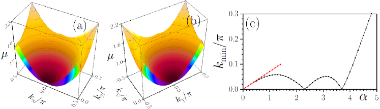
Figure 2: (a,b) Two different cuts of $\mu_{\mathrm{lin}}({\bm{k}})$ dependence in the first Brillouin zone at $\alpha=1$ (two lowest bands are shown), showing that the minimum of $\mu_{\mathrm{lin}}({\bm{k}})$ is achieved on the ring of radius $k_{\min}$. (c) The radius of the ring versus $\alpha$. The black curve is the numerical result, while the short red line shows the analytical prediction for $\alpha\ll\,\lambda,$ as given by equation (15). Note that, at large $\alpha,$ the radius $k_{\min}$ increases as $\alpha,$ as expected for the uniform SOC.

3 Symmetry properties of solitons

Now we turn to exact soliton solutions of equation (1) in the form of ${\bm{\Psi}}=e^{-i\mu t}\bm{\psi}(x,y)$, with $t$-independent complex spinor $\bm{\psi}=\left(\psi_{1}(x,y),\psi_{2}(x,y)\right)^{\mathrm{T}}.$ Thus, we consider the nonlinear eigenvalue problem:

$$\mu\bm{\psi}=H\bm{\psi}-\left(\bm{\psi}^{{\dagger}}\bm{\psi}\right)\bm{\psi},$$ (16)

where the linear part $H$ of the model’s Hamiltonian (1) is given by equation (4). The consideration below is limited to the case of a square lattice cell with equal $x-$ and $y-$periods: $\lambda_{x}=\lambda_{y}=\lambda$, and hence the general symmetry properties pertain to this choice. To describe families of nonlinear solutions (which in our case do not bifurcate from the linear limit), we first address the symmetries of $H$. To this end we introduce time reversal operator $\mathcal{T}$ acting on $\bm{\psi}$ as the complex conjugation, $\mathcal{T}\bm{\psi}=\bm{\psi}^{\ast}$, $x-$ and $y-$ spatial-inversion operators $\mathcal{P}_{x}$ and $\mathcal{P}_{y}$, acting as

$$\mathcal{P}_{x}\bm{\psi}(x,y)=\bm{\psi}(-x,y),\quad\mathcal{P}_{y}\bm{\psi}(x,y)=\bm{\psi}(x,-y),$$ (17)

as well as $\mathcal{P}=\mathcal{P}_{x}\mathcal{P}_{y}$ mapping, $(x,y)\rightarrow(-x,-y)$, the exchange operator,

$$J\bm{\psi}(x,y)=\bm{\psi}(y,x),$$ (18)

and two operators of translations by half-period along the $x$ and $y$ directions:

$$\tau_{x}\bm{\psi}(x,y)=\bm{\psi}(x+\pi/\lambda,y),\qquad\tau_{y}\bm{\psi}(x,y)=\bm{\psi}(x,y+\pi/\lambda).$$ (19)

Now we can identify the symmetries of $H$. First, $H$ is $\mathcal{PT}$-symmetric: $[H,\mathcal{PT}]=0$. The second symmetry, $\beta,$ commuting with the linear Hamiltonian, $[H,\beta]=0$, can be constructed as

$$\beta=\mathcal{P}_{x}J\left(\sigma_{0}+i\sigma_{2}\right)/\sqrt{2},\qquad\sigma_{0}+i\sigma_{2}=\left(\begin{array}[]{cc}1&1\\ -1&1\end{array}\right).$$ (20)

Using properties $\mathcal{P}_{x}J\mathcal{P}_{x}=\mathcal{P}_{y}J\mathcal{P}_{y}=\mathcal{P}J=J\mathcal{P}$, one can verify that $\beta$ is a generator of a cyclic group of order $8$ ($\beta^{8}=1$), which is isomorphic to $\mathbb{Z}_{8}$ [51, 52]. Both $\mathcal{PT}$ and $\beta$ symmetries do not contain shifts, hence they are referred to as local symmetries. Meantime we observe that there exists also the discrete translational symmetry over the primitive lattice vectors, i.e., ${\bm{u}}_{1}=(2,0)$ and ${\bm{u}}_{2}=(0,2)$ in our case, as well as the symmetries related to the shifts over half-period and defined as $\sigma_{3}{\cal P}_{x}\tau_{x}\tau_{y}$ and $\sigma_{1}{\cal P}_{y}\tau_{x}\tau_{y}$. Since here we are interested only in localized solutions, these lattice translations will not be considered.

Taking into account that $\beta^{4}=-1$, one identifies

$$\mathfrak{G}_{\mathrm{loc}}=\{\pm 1,\pm\mathcal{PT},\pm\mathcal{T}_{F},\pm\beta,\pm\beta^{2},\pm\beta^{3},\pm\beta\mathcal{PT},\pm\beta^{3}\mathcal{PT}\}$$ (21)

as the group of local symmetries of $H$. We emphasize that although the group $\mathfrak{G}_{\mathrm{loc}}$ is obtained for the particular choice of $\theta(x,y),$ the following analysis is not restricted to this choice and depends only on the group $\mathfrak{G}_{\mathrm{loc}},$ which can be realized for a broad variety of the $H-$Hamiltonians. In $\mathfrak{G}_{\mathrm{loc}}$ we use notation $\mathcal{T}_{\mathrm{F}}=\beta^{2}\mathcal{PT}=i\sigma_{2}\mathcal{T}$ for the spin-1/2 time reversal, and refer to elements with ”$+$” (”$-$”) sign as symmetries (anti-symmetries). Then, one can distinguish three cases as follows. If, for a given solution $\bm{\psi}$ of equation (16), there exists an element $g$ of $\mathfrak{G}_{\mathrm{loc}}$ such that $\bm{\psi}_{g}=g\bm{\psi}$ is a solution of equation (16) with the same $\mu$, we define $\bm{\psi}_{g}$ as a $g$-transformed solution. If, additionally, $\bm{\psi}_{g}=\bm{\psi}$ (or $\bm{\psi}=g\bm{\psi}$), such a solution is termed a $g$-symmetric one. If a given solution features $\bm{\psi}\neq g\bm{\psi}$ for all $g\in\mathfrak{G}_{\mathrm{loc}}$, then one says that symmetry breaking occurs. Although we cannot exclude a possibility of the symmetry breaking in our case, the extensive numerical studies of localized states of equation (16) have not revealed such a possibility. Therefore, we focus below on the existence and properties of ”symmetric” solutions, i.e., ones generated by all symmetry transformations from $\mathfrak{G}_{\mathrm{loc}}$.

Generally speaking, a symmetry of a linear Hamiltonian does not yet imply the symmetry of the complete nonlinear Hamiltonian. For a nonlinear solution to be generated by a symmetry $g$, the nonlinearity must be compatible with that symmetry. There exist two possibilities for that to occur [53]. Either the nonlinearity is $g$-symmetric, i.e., in our case, $[g,\bm{\psi}^{{\dagger}}\bm{\psi}]=0$ for any $\bm{\psi}$, or it is weakly $g$-symmetric, i.e., $\bm{\psi}^{{\dagger}}\bm{\psi}=(g\bm{\psi})^{{\dagger}}g\bm{\psi}$ is verified for a $g$-transformed solution $g\bm{\psi}$ (although not necessarily for any $\bm{\psi}$). It is straightforward to verify that the Manakov’s (SU(2)-symmetric) nonlinearity in equation (16) is weakly symmetric with respect to local elements of $\mathfrak{G}_{\mathrm{loc}}$. Therefore, below we look for nonlinear modes generated by the symmetry group $\mathfrak{G}_{\mathrm{loc}}$.

Using properties of the cyclic group of the $\beta$ transformations, one concludes that there exist no nontrivial $\beta^{n}$-symmetric solutions. Indeed, starting with $\beta^{2}$, the existence of $\beta^{2}$-symmetric solution $\bm{\psi}_{\beta^{2}}$ implies that $-\bm{\psi}_{\beta^{2}}=\beta^{4}\bm{\psi}_{\beta^{2}}=\beta^{2}\bm{\psi}_{\beta^{2}}=\bm{\psi}_{\beta^{2}}$, i.e., $\bm{\psi}_{\beta^{2}}\equiv 0$. Further, if a solution is $\beta$-symmetric, it is also $\beta^{2}$-symmetric, and hence is zero, too. These arguments are repeated for all $\pm\beta^{n}$-symmetries. Hence, $\beta^{n}$ transformation generates new solutions: if any solution $\bm{\psi}$ of (16) is found, then $\beta^{n}\bm{\psi}\neq\bm{\psi}$ (for $n=1,\ldots,7$) is another solution corresponding to the same $\mu$.

Not all symmetries from $\mathfrak{G}_{\mathrm{loc}}$ result in physically distinct solutions. For any symmetry involving antilinear time reversal $\mathcal{T}$, the anti-symmetry amounts to a trivial phase shift. For instance, if solution $\bm{\psi}_{\mathcal{PT}}$ is a $\mathcal{PT}$-symmetric one, then $i\bm{\psi}_{\mathcal{PT}}$ is anti-$\mathcal{PT}$-symmetric. Therefore, in the analysis of symmetric solutions of equation (16) presented below, we exclude all anti-symmetries. This leaves us with only four transformations: $\mathcal{PT}$, $\mathcal{T}_{F}$, $\beta\mathcal{PT}$, and $\beta^{3}\mathcal{PT}$, that may generate physically different solutions. Among these elements only the $\mathcal{PT}$-symmetry allows for symmetric solutions: $\bm{\psi}_{\mathcal{PT}}=\mathcal{PT}\bm{\psi}_{\mathcal{PT}}$. Now, let us consider $\bm{\psi}_{\mathcal{PT}}$ and its $\beta^{2}$-transformation: $\bm{\psi}_{\mathcal{T}_{F}}=\beta^{2}\bm{\psi}_{\mathcal{PT}}=\mathcal{T}_{F}\bm{\psi}_{\mathcal{PT}}=i\sigma_{2}\mathcal{P}\bm{\psi}_{\mathcal{PT}}$. One readily concludes that the absolute value of the first (second) component of $\bm{\psi}_{\mathcal{T}_{F}}$ is the $\mathcal{P}$-inverse absolute value of the second (first) component of $\bm{\psi}_{\mathcal{PT}}$. In this sense, these solutions are topologically similar. The topological similarity is also verified for the pair of $\beta\mathcal{PT}$- and $\beta^{3}\mathcal{PT}$-symmetric solutions related by the $\beta^{2}$ transformation. On the other hand, $\mathcal{PT}$- and $\beta\mathcal{PT}$-symmetric solutions have essentially different distributions of the fields in both components.

The above analysis is applicable for any family of localized nonlinear modes. Although the detailed analysis of numerically obtained families (fundamental, dipole-, and quadrupole-like) will be done in the next Section, here we can illustrate their main symmetry-related properties. These solitons, found by the Newton relaxation method, that permits obtaining entire families parameterized by the chemical potential $\mu,$ are characterized by their norm $U(\mu)$ and size $w(\mu)$, defined as:

$$U(\mu)\equiv\int\bm{\psi}^{{\dagger}}\bm{\psi}d^{2}r;\qquad w(\mu)\equiv{U(\mu)}\left[\int(\bm{\psi}^{{\dagger}}\bm{\psi})^{2}d^{2}r\right]^{-1/2}$$ (22)

and the peak amplitudes of spinor components $a_{1,2}(\mu)=\max\left|\psi_{1,2}\right|.$

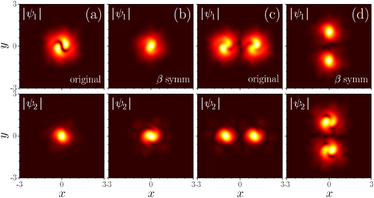
Figure 3: Examples of stable $\mathcal{PT}$-symmetric solutions and their $\beta$-transformations for the branches of fundamental (a,b) and dipole (c,d) solitons at $\mu=2$, $\alpha=3$.

In figure 3 we show $\mathcal{PT}$-symmetric solutions (panels (a) and (c)) and the respective $\beta$-transformed solutions (panels (b) and (d)) for the families of fundamental solitons (panels (a) and (b)) and dipoles (panels (c) and (d)). It is straightforward to verify that both $U(\mu)$ and $w(\mu)$ are equal for a given $\mathcal{PT}$-symmetric soliton and its $\beta^{n}$-transformation. It is also clear that the linear stability of a $\mathcal{PT}$-symmetric state coincides with the stability of its $\beta^{n}$ transformation: if $\bm{\psi}_{\mathcal{PT}}$ is stable (unstable), the same is valid for $\beta^{n}\bm{\psi}_{\mathcal{PT}}$. Therefore, the nonlinear modes shown in figures 3 (a) and (b) (and in figures 3 (c) and (d)) are either both linearly stable or both unstable, in the former case being stabilized by the nonlinearity.

4 Soliton families and their stability: numerical results

The simplest family of self-trapped solutions supported by the 2D helicoidal SOC landscape is represented by fundamental solitons. To be stable, such solitons have to be centered at a maximum of the periodic SOC phase, $\theta(x,y)=\pi,$ with the chemical potential taking values below the edge of the first band in the linear spectrum, i.e., at $\mu\leq\mu_{\mathrm{be}}$ [see the dashed line in figure 4(a)]. The dominant component (either $\psi_{1}$ or $\psi_{2}$, see Sec. 3) of such a soliton typically has a bell-shaped profile with weak modulations on the top of it, while a weaker component may feature a very complex profile with curved nodal lines, see, e.g., figure 4(c). Both components of the wave function have nontrivial phase distributions, as shown in the insets of figure 4(c). When the chemical potential approaches the bottom of the first linear band, the soliton expands and its width diverges, see a representative $w(\mu)$ dependence in figure 4(a). In this regime, spatial modulations of the soliton shape become much more pronounced for both components [figure 4(d)]. Peak amplitudes $a_{1,2}(\mu)$ of both components decrease with the increase of $\mu$ and vanish exactly at the edge of the allowed band [figure 4(a)]. In contrast, the soliton’s norm, $U(\mu),$ shows a non-monotonous behavior, clearly indicating that solitons exist only above a certain threshold value of the norm. This threshold decreases with the increase of the SOC strength $\alpha$. At $\alpha\rightarrow 0$, the dependence $U(\mu)$ approaches a constant value, $U_{T}\approx 5.85$, which is the above-mentioned Townes’ soliton norm [19, 20, 32].

The growth of deformation and non-monotonous character of the $U(\mu)$ dependence appearing with the increase of $\alpha$ suggests that the helicoidal SOC may play a stabilizing role for fundamental solitons. We have checked the stability of such states by simulating equation (1) with small input complex noise added to stationary profiles, up to very large times. As a result, it was found that large parts of $U(\mu)$ families, with negative slope $\partial U(\mu)/\partial\mu$, represent stable fundamental solitons. These findings are summarized in the existence-and-stability diagram displayed in figure 4(b), where the solitons exist at $\mu\leq\mu_{\mathrm{be}}$, and are stable for all values of $\mu\leq\mu_{\mathrm{cr}}$, the border of the stability domain exactly corresponding to the $\left.\partial U(\mu)/\partial\mu\right|_{\mu=\mu_{\mathrm{cr}}}=0$ boundary, in agreement with the well-known Vakhitov-Kolokolov criterion [19, 20, 54].

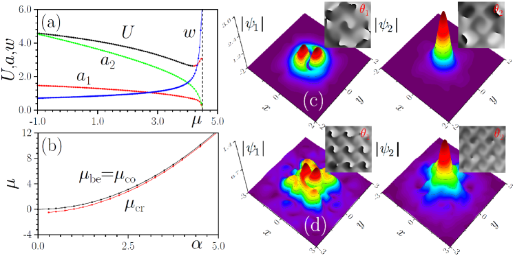
Figure 4: (a) Norm $U(\mu)$, size $w(\mu)$, and component amplitudes, $a_{1,2}(\mu)$, of fundamental solitons versus chemical potential $\mu$ at $\alpha=3$. Black and red segments in the $U(\mu)$ dependence correspond to stable and unstable states, respectively. The dashed line shows the location of the bottom of the first band. (b) Existence and stability domains of the fundamental solitons in the $(\alpha,\mu)$ plane. The solitons exist at $\mu\leq\mu_{\mathrm{be}}=\mu_{\mathrm{co}}$, and are stable at $\mu\leq\mu_{\mathrm{cr}}$. Panels (c) and (d) display examples of profiles of the absolute value and phase (insets) of the fundamental solitons with $\mu=1$ (c, stable) and $\mu=4.2$ (d, taken at the stability border) are shown for $\alpha=3$.

The existence of stable fundamental solitons residing at the maxima of the periodic $\theta(x,y)$ function suggests that equation (1) allows to construct complexes of the solitons, which cannot be done with the help of spatially-uniform SOC [29, 33, 34]. We have found that it is indeed possible to create stable complexes of spatially separated solitons with opposite signs of ${\bm{\psi}}$, i.e., dipoles and quadrupoles.

Examples of the simplest dipole soliton complex, that may be considered as a pair of two solitons with opposite signs, and properties of dipole families are presented in figure 5. The dipole is built of two soliton-like density maxima placed at adjacent maxima of $\theta(x,y)$ and, accordingly, separated by distance $\approx 2\pi/\lambda=2.$ The solitons interact through their tails, the interaction getting stronger with the increase of chemical potential $\mu$, due to weakening localization of each soliton [cf. figures 5(c) and (d)]. Even though phase distributions in the dipole modes are quite complex, due to spatially dependent SOC, one can see in the insets that the two density maxima in both components have, “on average”, phase shifts of $\pi$, which corresponds to the opposite signs of the two solitons. Because dipole solitons are excited nonlinear states, their chemical potential does not reach the bottom of the band. Instead, the dipoles exist below a certain cutoff value, $\mu=\mu_{\mathrm{co}}$, whose $\alpha-$dependence is shown in figure 5(b) by the blue line. At the cutoff position, amplitudes of both components of the dipole’s wave function, $\psi_{1,2}$, do not vanish, and the width remains finite, but dependence $U(\mu)$ acquires a vertical tangential direction [for illustrative purposes, in figure 5(a) we plot half of total norm, as it is comparable with that of fundamental soliton]. Because the capability of SOC landscape to compensate repulsive forces acting between solitons with opposite signs reduces with the decrease of $\alpha$, the cutoff value $\mu_{\mathrm{co}}$ rapidly decreases at $\alpha\rightarrow 0$ [figure 5(b)].

An important finding is that the dipole solitons enabled by helicoidal SOC may be stable. The stabilization is possible below a critical value of the chemical potential, $\mu\leq\mu_{\mathrm{cr}}$ [see the stable (black) segment of the $U(\mu)$ branch in figure 5(a)], while, close to the cutoff, the dipoles are unstable [see the red segment of the $U(\mu)$ branch]. The entire existence and stability domains for the dipole solitons is presented in figure 5(b): they exist at $\mu\leq\mu_{\mathrm{co}}$, and are stable at $\mu\leq\mu_{\mathrm{cr}}$. In the instability domain, the most typical destabilization mechanism is spontaneous breakup of symmetry between two density maxima, accompanied by oscillations with a growing amplitude, leading to the collapse or formation of a fundamental soliton.

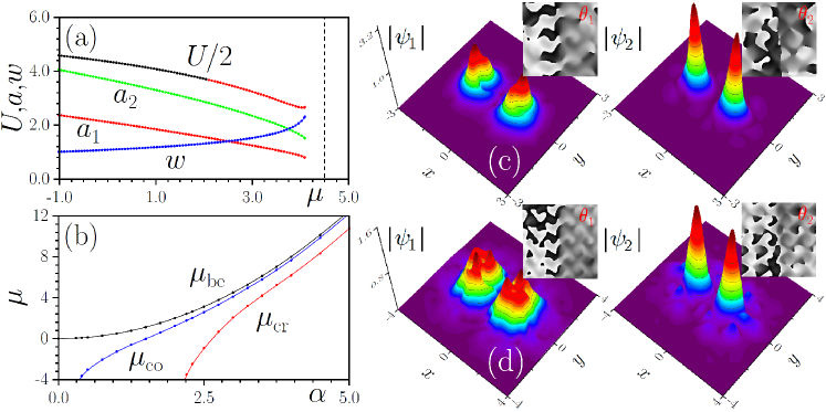
Figure 5: (a) The norm $U(\mu)$, size $w(\mu)$, and component amplitudes, $a_{1,2}(\mu)$, of dipole solitons versus chemical potential $\mu$ at $\alpha=3$. Black and red segments in the $U(\mu)$ dependence correspond to stable and unstable states, respectively. The dashed line shows the location of the bottom level of the first band. (b) Existence and stability domains of the dipole solitons in the $(\alpha,\mu)$ plane. They exist at $\mu\leq\mu_{\mathrm{co}}<\mu_{\mathrm{be}}$, and are stable at $\mu\leq\mu_{\mathrm{cr}}$. Panels (c) and (d) display examples of profiles of the absolute value and phase (insets) of dipole solitons with $\mu=1$ (c, stable) and $\mu=4$ (d, unstable) for $\alpha=3$. For convenience for dipole solitons the SOC profile was shifted by half of the period $\pi/\lambda$ along the $x$-axis.

Finally, we have found quadrupole soliton complexes, composed of four solitons with alternating signs of ${\bm{\psi}}$, residing at neighboring maxima of $\theta(x,y)$. Examples of quadrupoles and properties of their families are presented in figure 6. Note that in such states diagonal pairs of solitons have identical signs. In the course of the evolution, such pairs of mutually attractive solitons may fuse, destroying the whole structure. For this reason, such states are more fragile than their dipole counterparts, and the stability region for them is narrower, with a more complex shape. Quadrupoles also exist below the respective cutoff value of the chemical potential, $\mu\leq\mu_{\mathrm{co}}$, see figure 6(a,b).

Due to the complexity of the stability domain, we were able to identify it only for a limited set of values of the SOC strengths, $\alpha.$ For instance, in figure 6(b) the quadrupoles are stable between two upper red dots, and also below the lower one. Stable segments of the $U(\mu)$ dependence in figure 6(a) are black ones. This stability was found solely in a limited range, $3\lesssim\alpha\lesssim 4$, but not for larger SOC strengths.

Finally, in addition to the dipoles and quadrupoles, it is possible to construct multipole states arranged into lines, which are more stable than the quadrupoles.

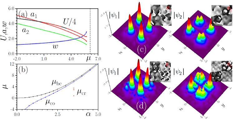
Figure 6: (a) The norm $U(\mu)$, size $w(\mu)$, and component amplitudes, $a_{1,2}(\mu)$, of quadrupole solitons versus chemical potential $\mu$ at $\alpha=3.5$. Black and red segments in the $U(\mu)$ dependence correspond to stable and unstable states, respectively. (b) Existence and stability domains of the quadrupole solitons in the $(\alpha,\mu)$ plane. They exist at $\mu\leq\mu_{\mathrm{co}}<\mu_{\mathrm{be}}$. Since the shape of the stability domain is very complex, in panel (b) we only show borders of the stability domain at $\alpha=3.5$. Panels (c) and (d) display examples of profiles of the absolute value and phase (insets) of quadrupoles with $\mu=3$ (c, stable) and $\mu=5.6$ (d, unstable) for $\alpha=3.5$. For convenience for quadrupole solitons the SOC profile was shifted by half of the period $\pi/\lambda$ along both $x$- and $y$-axes.

5 Conclusions

In this work, we have introduced a 2D system which includes the cubic self-attraction and SOC (spin-orbit coupling) subject to the spatially-periodic modulation, as a physically relevant dynamical model of BEC in the binary ultracold bosonic gas. The system gives rise to two-component (pseudo-spinor) fundamental solitons in a vast region of the corresponding parameter space. It also essentially expands the variety of stable self-trapped modes in the 2D setting by the creation of families of robust dipole and quadrupole states built of two or four fundamental-like solitons with alternating signs of the wavefunction. Stability of these solutions and properties of their families, such as the norm, widths, and amplitudes, have been analyzed, parameterizing the families by the chemical potential. We have also shown that, for each species of the localized state (fundamental, dipole, or quadrupole), additional solutions can be generated from a given one by symmetry operations forming an Abelian eight-element group.

These results may be extended by considering axially symmetric (radial) patterns of the spatial SOC modulation, instead of the periodic lattice patterns. In the axisymmetric system, it may be interesting, in particular, to consider azimuthal mobility of solitons and interactions between them. A challenging possibility is to develop a three-dimensional generalization of the system with the spatially periodic SOC modulation.

Acknowledgements

B.A.M. is supported, in part, by the Israel Science Foundation through grant No. 1286/17, and by grant No. 2015616 from the joint program of Binational Science Foundation (US-Israel) and National Science Foundation (US). V.V.K. acknowledges financial support from the Portuguese Foundation for Science and Technology (FCT) under Contract no. UIDB/00618/2020. E.Y.S. acknowledge support by the Spanish Ministry of Science and the European Regional Development Fund through PGC2018-101355-B-I00 (MCIU/AEI/ FEDER, UE) and the Basque Country Government through Grant No. IT986-16. This work was partially supported by the program 1.4 of Presidium of the Russian Academy of Sciences ”Topical problems of low temperature physics”.

References

References

- [1] Dresselhaus G 1955 Spin-orbit coupling effects in zinc blende structures Phys. Rev. 100 580
- [2] Bychkov Y A and Rashba E I 1984 Oscillatory effects and the magneto-sussceptibility of carriers in inversion layers J. Phys. C 17 6039
- [3] Fabian J, Matos-Abiague A, Ertler C, Stano P and Žutic I 2007 Semiconductor spintronics Acta Physica Slovaca 57 565
- [4] Manchon A, Koo H G, Nitta J, Frolov S M and Duine R A 2015 New perspectives for Rashba spin-orbit coupling Nature Materials 14 871
- [5] Galitski V and Spielman I B 2013 Spin-orbit coupling in quantum gases Nature 494 49
- [6] Goldman N, Juzeliunas G, Öhberg P and Spielman I B 2014 Light-induced gauge fields for ultracold atoms Rep. Progr. Phys. 77 126401
- [7] Zhai H 2015 Degenerate quantum gases with spin–orbit coupling: a review Rep. Progr. Phys. 78 026001
- [8] Zhang Y, Mossman M E, Busch T, Engels P and Zhang C 2016 Properties of spin-orbit-coupled Bose-Einstein condensates Front. of Phys. 11 118103
- [9] Malomed B A 2018 Creating solitons by means of spin-orbit coupling EPL 122 36001 (An invited Perspective mini-review; included in Highlights of 2018)
- [10] Achilleos V, Frantzeskakis D J, Kevrekidis P J and Pelinovsky D E 2013 Matter-wave bright solitons in spin-orbit coupled Bose-Einstein condensates Phys. Rev. Lett. 110, 264101
- [11] Kartashov Y V, Konotop V V and Abdullaev F Kh 2013 Gap solitons in a spin-orbit-coupled Bose-Einstein condensate Phys. Rev. Lett. 111 060402
- [12] Xu Y, Zhang Y and Wu B 2013 Bright solitons in spin-orbit-coupled Bose-Einstein condensates Phys. Rev. A 87 013614
- [13] Salasnich L and Malomed B A 2013 Localized modes in dense repulsive and attractive Bose-Einstein condensates with spin-orbit and Rabi couplings Phys. Rev. A 87 063625
- [14] Kartashov Y V, Konotop V V and Zezyulin D A 2014 Bose-Einstein condensates with localized spin-orbit coupling: Soliton complexes and spinor dynamics Phys. Rev. A 90 063621
- [15] Kartashov Y V and Konotop V V 2017 Solitons in Bose-Einstein Condensates with Helicoidal Spin-Orbit Coupling Phys. Rev. Lett. 118 190401
- [16] Kartashov Y V, Konotop V V, Modugno M and Sherman E Ya 2019 Solitons in inhomogeneous gauge potentials: Integrable and nonintegrable dynamics Phys. Rev. Lett. 122 064101
- [17] Wu Z, Zhang L, Sun W, Xu X-T, Wang B-Z, Ji S-J, Deng Y, Chen S, Liu X-J and Pan J-W 2016 Realization of two-dimensional spin-orbit coupling for Bose-Einstein condensates Science 354 83
- [18] V. E. Lobanov, Y. V. Kartashov and V. V. Konotop 2014 Fundamental, multipole, and half-vortex gap solitons in spin-orbit coupled Bose-Einstein condensates Phys. Rev. Lett. 112 180403
- [19] L. Bergé 1998 Wave collapse in physics: principles and applications to light and plasma waves Phys. Rep. 303 259
- [20] Fibich G The Nonlinear Schrödinger Equation: Singular Solutions and Optical Collapse (Springer: Heidelberg, 2015)
- [21] Dias J-P, Figueira M and Konotop V V 2015 Coupled Nonlinear Schrödinger Equations with a Gauge Potential: Existence and Blowup Stud. Appl. Math. 136 241
- [22] Malomed B A 2016 Multidimensional solitons: Well-established results and novel findings Eur. Phys. J. Special Topics 225 2507
- [23] Kartashov Y V, Astrakharchik G E, Malomed B A and Torner L 2019 Frontiers in multidimensional self-trapping of nonlinear fields and matter Nature Reviews Physics 1 185
- [24] Baizakov B B, Malomed B A and Salerno M 2004 Multidimensional solitons in a low-dimensional periodic potential Phys. Rev. A 70 053613
- [25] Yang J and Musslimani Z H 2003 Fundamental and vortex solitons in a two-dimensional optical lattice Opt. Lett. 28 2094
- [26] Sakaguchi H and Malomed B A 2005 Higher-order vortex solitons, multipoles, and supervortices on a square optical lattice. Europhys. Lett. 72 698
- [27] Vuong L T, Grow T D, Ishaaya A, Gaeta A L, ’t Hooft G W, Eliel E R and Fibich G 2006 Collapse of optical vortices Phys. Rev. Lett. 96 133901
- [28] Malomed B A 2019 Vortex solitons: Old results and new perspectives Physica D 399 108
- [29] Sakaguchi H, Li B and Malomed B A 2014 Creation of two-dimensional composite solitons in spin-orbit-coupled self-attractive Bose-Einstein condensates in free space Phys. Rev. E 89 032920
- [30] Mardonov Sh, Sherman E Ya, Muga J G, Wang H-W, Ban Y and Chen X 2015 Collapse of spin-orbit-coupled Bose-Einstein condensates Phys. Rev. A 91 043604
- [31] Manakov S V 1973 On the theory of two-dimensional stationary self-focusing of electromagnetic waves Zh. Eksp. Teor. Fiz. 65 505 [English translation: Sov. Phys. JETP 38, 248 (1974)]
- [32] Chiao R Y, Garmire E and Townes C H 1964 Self-trapping of optical beams Phys. Rev. Lett. 13 479
- [33] Sakaguchi H, Sherman E Ya and Malomed B A 2016 Vortex solitons in two-dimensional spin-orbit coupled Bose-Einstein condensates: Effects of the Rashba-Dresselhaus coupling and the Zeeman splitting Phys Rev. E 94 032202
- [34] Sakaguchi H and Malomed B A 2018 One- and two-dimensional gap solitons in spin-orbit-coupled systems with Zeeman splitting Phys. Rev. A 97 013607
- [35] Li Y, Luo Z, Liu Y, Chen Z, Huang C, Fu S, Tan H and Malomed B A 2017 Two-dimensional solitons and quantum droplets supported by competing self- and cross-interactions in spin-orbit-coupled condensates New J. Phys. 19 113043
- [36] Lee T D, Huang K and Yang C N 1957 Eigenvalues and eigenfunctions of a Bose system of hard spheres and its low-temperature properties Phys. Rev. 106 1135
- [37] Petrov D S 2015 Quantum mechanical stabilization of a collapsing Bose-Bose mixture Phys. Rev. Lett. 115 155302
- [38] Petrov D S and Astrakharchik G E 2016 Ultradilute low-dimensional liquids Phys. Rev. Lett. 117 100401
- [39] Ferrier-Barbut I, Kadau H, Schmitt M, Wenzel M and Pfau T 2016 Observation of quantum droplets in a strongly dipolar bose gas Phys. Rev. Lett. 116 215301
- [40] Chomaz L, Baier S, Petter D, Mark M J, Wachtler F, Santos L and Ferlaino F 2016 Quantum-uctuation-driven crossover from a dilute Bose-Einstein condensate to a macrodroplet in a dipolar quantum fluid Phys. Rev. X 6 041039
- [41] Cabrera C, Tanzi L, Sanz J, Naylor B, Thomas P, Cheiney P and Tarruell L 2018 Quantum liquid droplets in a mixture of Bose-Einstein condensates Science 359 301
- [42] Semeghini G, Ferioli G, Masi L, Mazzinghi C, Wolswijk L, Minardi F, Modugno M, Modugno G, Inguscio M and Fattori M 2018 Self-Bound Quantum Droplets of Atomic Mixtures in Free Space Phys. Rev. Lett. 120 235301
- [43] Zhang Y-C, Zhou Z-W, Malomed B A and Pu H 2015 Stable solitons in three-dimensional free space without the ground state: Self-trapped Bose-Einstein condensates with spin-orbit coupling Phys. Rev. Lett. 115, 253902
- [44] Kartashov Y V, Torner L, Modugno M, Sherman E Ya, Malomed B A and Konotop V V 2020 Multidimensional hybrid Bose-Einstein condensates stabi-lized by lower-dimensional spin-orbit coupling Phys. Rev. Res. 2 013036
- [45] Li Y, Zhang X, Zhong R, Luo Z, Liu B, Huang C, Pang W and Malomed B A 2019 Two-dimensional composite solitons in Bose-Einstein condensates with spatially confined spin-orbit coupling Comm. Nonlin. Sci. Num. Sim. 73 481
- [46] García-Ripoll J J, Pérez-García V M and Vekslerchik V 2001 Construction of exact solutions by spatial translations in inhomogeneous nonlinear Schrödinger equations Phys. Rev. A 64 056602
- [47] M. Merkl, A. Jacob, F. E. Zimmer, P. Öhberg and L. Santos 2010 Chiral Confinement in Quasirelativistic Bose-Einstein Condensates Phys. Rev. Lett. 104 073603
- [48] Kartashov Y V and Konotop V V 2020 Stable Nonlinear Modes Sustained by Gauge Fields Phys. Rev. Lett. 125, 054101
- [49] Kartashov Y V, Malomed B A, Konotop V V, Lobanov V E and Torner L 2015 Stabilization of spatiotemporal solitons in Kerr media by dispersive coupling Opt. Lett. 40 1045
- [50] Abramowitz M and Stegun I Handbook of Mathematical Functions: with Formulas, Graphs, and Mathematical Tables (Dover Books on Mathematics, 1965)
- [51] Knox R S and Gold A Symmetry in the Solid State (W. A. Benjamin, New York, 1964)
- [52] Kurzweil H and Stellmacher B The Theory of Finite Groups: An Introduction (Springer, Heidelberg, 2004)
- [53] Zezyulin D A and Konotop V V 2013 Stationary modes and integrals of motion in nonlinear lattices with a -symmetric linear part J. Phys. A: Math. Theor. 46 415301
- [54] Vakhitov N G and Kolokolov A A 1973 Stationary solutions of the wave equation in a medium with nonlinearity saturation Radiophys. Quantum Electron. 16 783