Robust calibration of multiparameter sensors via machine learning at the single-photon level
Abstract
Calibration of sensors is a fundamental step to validate their operation. This can be a demanding task, as it relies on acquiring a detailed modelling of the device, aggravated by its possible dependence upon multiple parameters. Machine learning provides a handy solution to this issue, operating a mapping between the parameters and the device response, without needing additional specific information on its functioning. Here we demonstrate the application of a Neural Network based algorithm for the calibration of integrated photonic devices depending on two parameters. We show that a reliable characterization is achievable by carefully selecting an appropriate network training strategy. These results show the viability of this approach as an effective tool for the multiparameter calibration of sensors characterized by complex transduction functions.
I Introduction
Quantum metrology has demonstrated significant advances in the last few years, keeping up with the perspective of a novel generation of quantum sensors with enhanced sensitivity Paris (2009); Giovannetti et al. (2011); Pezzé and Smerzi (2014); Pirandola et al. (2018); Polino et al. (2020). In order to fully exploit these advantages, the device must be known and controlled, so that the measured parameters can be retrieved with good accuracy. This ability then relies on the availability of a trusted calibration of the sensor in hand Gianani et al. (2020). Conventional methods for device characterisation require, in general, a large set of calibration data and intensive post-processing. Alternatively, one could rely on refined a-priori physical models of the sensors, including noise effects, based on measured quantities. Such intensive approaches, however, become unpractical for sensors of increasing complexity, and unfeasible in the perspective of commercial devices.
Further, in realistic sensors, the user has typically access and control over a set of physical parameters, which in turn modify the internal characteristics of the device. Therefore, the target parameters are not directly evaluated, but inferred from measured quantities. Optical phases, determined by electrical signals via thermo-optic effects, are a case in point Flamini et al. (2015); Carolan et al. (2015); Harris et al. (2017); Taballione et al. (2019): here, voltages are the parameters of interest, but the measured optical signal derives from variations of optical phases. Therefore, the sensor inherently works as a transductor, mapping the parameters to be estimated onto measured quantities through a suitable response function, which needs to be characterized as well. In this respect, spurious effects also concur to determining the response function, and must be taken into account. This poses major difficulties in the modelling, and increases the complexity of an experimental characterisation via conventional methods.
A practical approach thus requires a different methodology for sensor calibration. A viable direction is provided by machine learning techniques, capable of handling large datasets and of solving tasks for which they have not been explicitly programmed; applications range from stock prices predictions Ticknor (2013); Enke et al. (2011) to the analysis of medical diseases Ganesan et al. (2010). In the last few years, several applications of machine learning methods in the quantum domain have been reported Dunjko and Briegel (2018); Mehta et al. (2019); Carleo et al. (2019), including state and unitary tomography Spagnolo et al. (2017); Carrasquilla et al. (2019); Palmieri et al. (2020); Rocchetto et al. (2019); Arrazola et al. (2019); Giordani et al. (2020); Neugebauer et al. (2020); Torlai et al. (2019); Tiunov et al. (9482), design of quantum experiments Nichols et al. (2019); Melnikov et al. (2018); Krenn et al. (2016); O’Driscoll et al. (2019); Sabapathy et al. (2019); Krenn et al. (2020); Gao et al. (2020), validation of quantum technology Agresti et al. (2019); Flamini et al. (2019); Knott (2016), identification of quantum features Cimini et al. (2020); Gebhart and Bohmann (2020), and the adaptive control of quantum devices Hentschel and Sanders (2010, 2011); Lovett et al. (2013); Bonato et al. (2016); Palittapongarnpim et al. (2017); Liu and Yuan (2017); Paesani et al. (2017); Lumino et al. (2018); Palittapongarnpim and Sanders (2019); Dinani et al. (2019); Liu et al. (2020); Peng and Fan (2020); Rambhatla et al. (2020); Valeri et al. (2020); Craigie et al. (2020); Nolan et al. (2020); Fiderer et al. (2020). Also, photonic platforms can be exploited for the realization of machine learning protocols Bernstein et al. (2020); Flamini et al. (2020). Recently, a first insight on the application of machine learning methods for the calibration of a quantum sensor has been reported Cimini et al. (2019). In detail, the characterization of an optical phase sensor was carried out by means of artificial neural networks (NNs) Haykin (2009). This has demonstrated its advantages, in that it required no detailed model, it relied on the same states for the calibration as for the estimation, and demonstrated robustness to finite-size datasets when compared to standard methods. When extending the use of NNs to multiple parameter scenarios, it can be expected that all these features can be preserved. However, conjugating this approach with the peculiarities of multiparameter estimation is far from obvious.
In this article, we demonstrate the calibration of multiphase sensors implemented in a femtosecond-laser-written photonic platform. The devices are multiarm interferometers with multiple embedded phases, which are controlled externally by applying a voltage to resistors placed within the sensor. We report on how to build and train a NN to make it capable to work as a reliable and practical calibration tool. Indeed, we show the requirements on the training process, in terms of the size of the dataset, as well as the need to resolve possible ambiguities which result from the non-monotonicity of the sensor response function. Our results give evidence on the viability of a machine learning approach for calibration of complex quantum devices.
II results
In this section, we detail our use of a feed-forward neural network Aggarwal (2018) to approximate the multivariate function that links single-photon detection probabilities, relative to outputs of an integrated three-mode device, given a certain input, to the voltage settings controlling the interferometer phases.
Regression is one of the most common problems faced by supervised learning algorithms. It consists in finding a map that links an input vector of features to the respective output vector consisting of real numbers, for all the examples in the dataset. NNs are very effective at modelling complex non-linear functions for very large dimension dataset described by many features, and their performances are particularly good when large training dataset, containing many different examples, are available.
II.1 Experimental platform
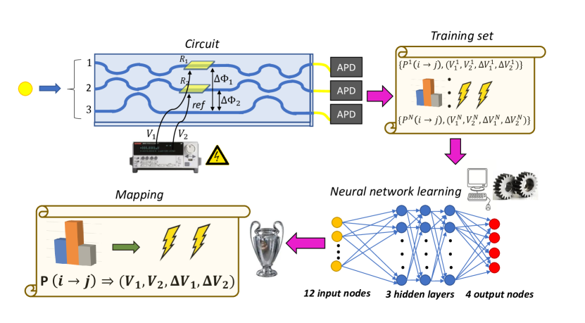
The integrated device under study is a three-arm interferometer realized by the femtosecond laser writing technique Gattass and Mazur (2008); G. Della Valle and R. Osellame and P. Laporta (2008) and able to perform multiphase estimation protocols Polino et al. (2019); Valeri et al. (2020). The circuit is composed by a sequence of two three-arm beam splitters (tritters) realized through a two-dimensional geometry decomposition and interposed by three internal arms encoding two independent optical phase shifts of two arms with respect to the third one (reference). These are thermo-optic phase shifts that can be tuned by means of ohmic resistors. When a set of voltages is applied to the resistors, a different global phase shift is generated along each optical path, thus changing the action of the device. A scheme of the device is reported in Fig. 1. The chip is studied in the single-photon regime. Pairs of photons with wavelength nm are generated by spontaneous parametric down conversion process in a
barium borate (BBO) crystal. A single photon of the pair is coupled into a fiber array connected to one of the circuit’s inputs, while the other photon acts as a trigger. Single-photon detectors are placed at the output fibers of the device and coincidence events between the trigger and the photon injected inside the chip are recorded. In this way, single-photon probabilities for each output () are measured by changing the input arm of the single-photon state and tuning the power dissipated on the internal resistors. In particular, we tune the voltages applied to each resistor independently, while keeping the others off. Due to the resistance dependence on its temperature and due to the thermal crosstalk between resistances, a given pair of voltages, applied on the thermo-resistors and respectively, implies a variation of the two phases described by the following approximate response function containing linear and quadratic dependencies from the dissipated power:
| (1) |
where the dissipated power is using Ohmic approximation for the two resistors, while and are, respectively, the linear and non-linear response coefficients associated to the phase shift when dissipating power on resistor .
The two voltages and are thus directly mapped into the two physical relative phase-shifts and . In standard characterisation, a theoretical model of the circuit allows to recover the likelihood describing the output probabilities through a fit of the measured probabilities. This, in turn, allows to extrapolate dynamic and static parameters of the chip Polino et al. (2019); Valeri et al. (2020). The aim of this work is to avoid relying on knowledge about both the theoretical model of circuit and the response function in Eq. (1). In fact, this would prove inefficient for the characterisation of mass-produced devices. The goal, instead, is to generate a mapping between voltages and output probabilities using only a limited set of measurements. We exploit the NN approach exactly to realize such goal (Fig. 1).
II.2 Neural network architecture and performances
We start using simulated data to inspect the algorithm requirements both in terms of network architecture and amount of training data needed to obtain good performances when evaluating new examples. This preliminary step has the only purpose of identifying more efficiently the structure of the NN for the calibration of a general three-arm interferometer. Therefore, a likelihood function describing exactly the device is not needed; the simulated data represent roughly its typical approximate likelihood. In our case the simulated data are obtained based on single-photon input-output probabilities estimated from experimental measurements through a maximum-likelihood technique. To train the NN, data are divided in a vector of input features corresponding to the input-output probabilities obtained when applying a given pair of controlled voltages, which constitute the elements of the output vector :
| (2) |
The index refers to each training example and represents the total number of training data. The vector of probabilities is constructed using counts extracted from a Poisson distribution whose mean values correspond to those assessed from the maximum-likelihood reconstruction. This procedure is needed for the NN to properly account for the presence of such source of uncertainty. A part of the data, viz. 15% of the whole set, is used as a validation set: it is not directly employed for the training, but rather to obtain an independent estimate on the training error. This is necessary to avoid overfitting.
We have tested different NN architectures with a different number of hidden layers and neurons per layer, studying the network performances for different activation functions, initialization parameters and optimization algorithms. Finally, we have chosen the one which obtains the smallest Root Mean Squared Error (RMSE) on the validation set. We notice that the full set of probabilities is redundant for the network training and satisfactory results can indeed be achieved training the network with only of them, obtained when injecting a photon respectively in the first and second input of the device. The training consists in tuning the model’s parameters to minimize the RMSE associated to each example of the training set; for this purpose the gradient of the loss function, corresponding to the summation of the RMSE over all the training examples, with respect to all the network’s parameters is computed using the backpropagation method Goodfellow et al. (2016). In the next step the gradient is used to minimize the loss function using the optimization algorithm Adam Kingma and Ba (2014).
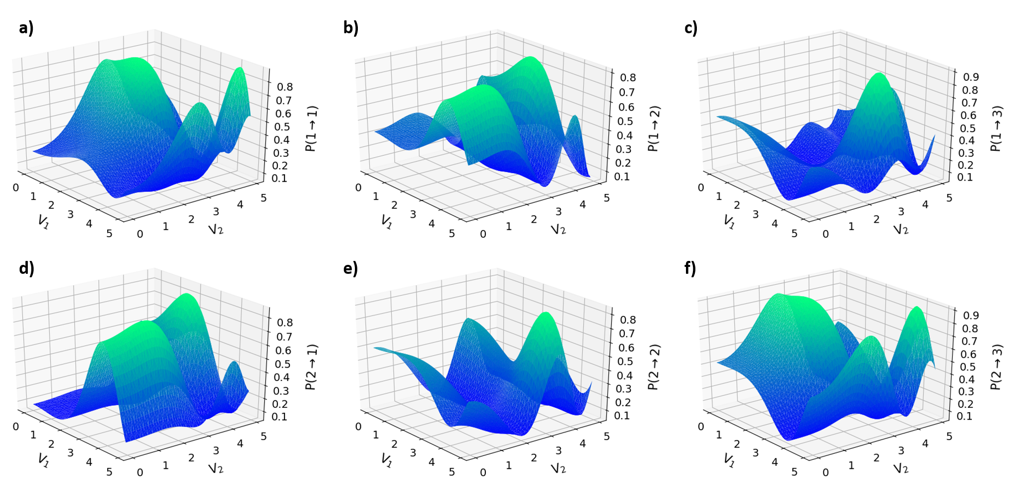
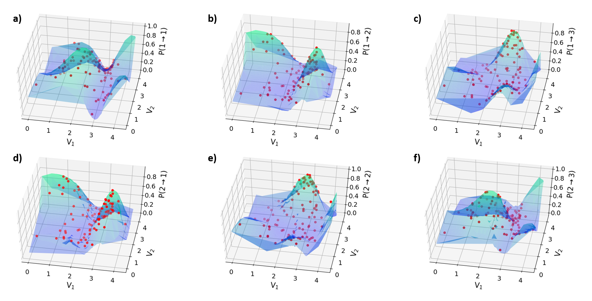
We train the network with the results obtained after the application of different tensions values to each of the two resistors in the device. This gives a tension grid with different tension pairs associated to the relative input-output probabilities available to train the network. Therefore, each example in the training set, consists in the tensions pairs associated to probability values. The trends of the values predicted by the trained-NN are reported in Fig. 2 as a function of the applied voltages on the two resistors. However, to obtain a good estimation in the full range of accessible tensions, it was necessary to incorporate into each training example the further set of probabilities , to which we refer as kicks, as follows:
| (3) |
where the values are added by considering the probabilities obtained by changing of a fixed value and the length of the and vectors is . This is necessary to remove ambiguities in the evaluation of the overall function, providing additional information to the network. More specifically, such requirement is due to the non-monotonicity of the output probabilities, resulting in the presence of multiple parameter points that correspond to the same probability values. Thus, in absence of additional data sets it is not possible to distinguish between those points. Comparing the network results on the validation set, the RMSE improves by thanks to the additional information provided with the tension kick, when evaluated in the full range of tension values. The advantage obtained is independent from the specific value of and , as long as they are large enough to give information about different regions of the inspected functions. Enlarging the data in each training example requires to increase the number of nodes in the input and output layers of the network. The architecture that allows to achieve the best performances, among the ones considered, is a network with input nodes and output ones separated by hidden layers with nodes each (Fig. 1). All the nodes, except the output ones which are activated by a linear function, are activated by a rectified linear unit function initializing their weights with random values extracted from a normal distribution centred in zero and with variance , where is the number of neurons in the previous layer.
We stop the training after epochs since the loss function on the validation set stops decreasing. To analyze the variability among different trainings, we study the results obtained, starting from the same datasets, after performing independent trainings of the network. The mean value of the Normalized Root Mean Squared Error (NRMSE) is given by:
| (4) |
where indicates the Euclidean norm. It is calculated on the validation set in such configuration obtaining a value of . After the network has been trained, its performances have been evaluated on an independent test set of different examples selected randomly among the possible tensions pairs of the , adding Poissonian noise on the detection events determining the probabilities values. Notably, since both the training and the test data include by random Poissonian noise, the resulting NN is robust when evaluating new noisy examples. To quantify how close the network estimation of the tension values is to the true ones, we evaluate the cosine similarity between the vector of network outputs , corresponding to the tensions for all the test examples, and the expected results , as follows:
| (5) |
which is equal to , when the prediction is equal to the true value . Moreover, to estimate how much the cosine similarity depends on the random sample selected, we compute its value on repetitions each containing examples extracted randomly among the available ones, obtaining a value of .
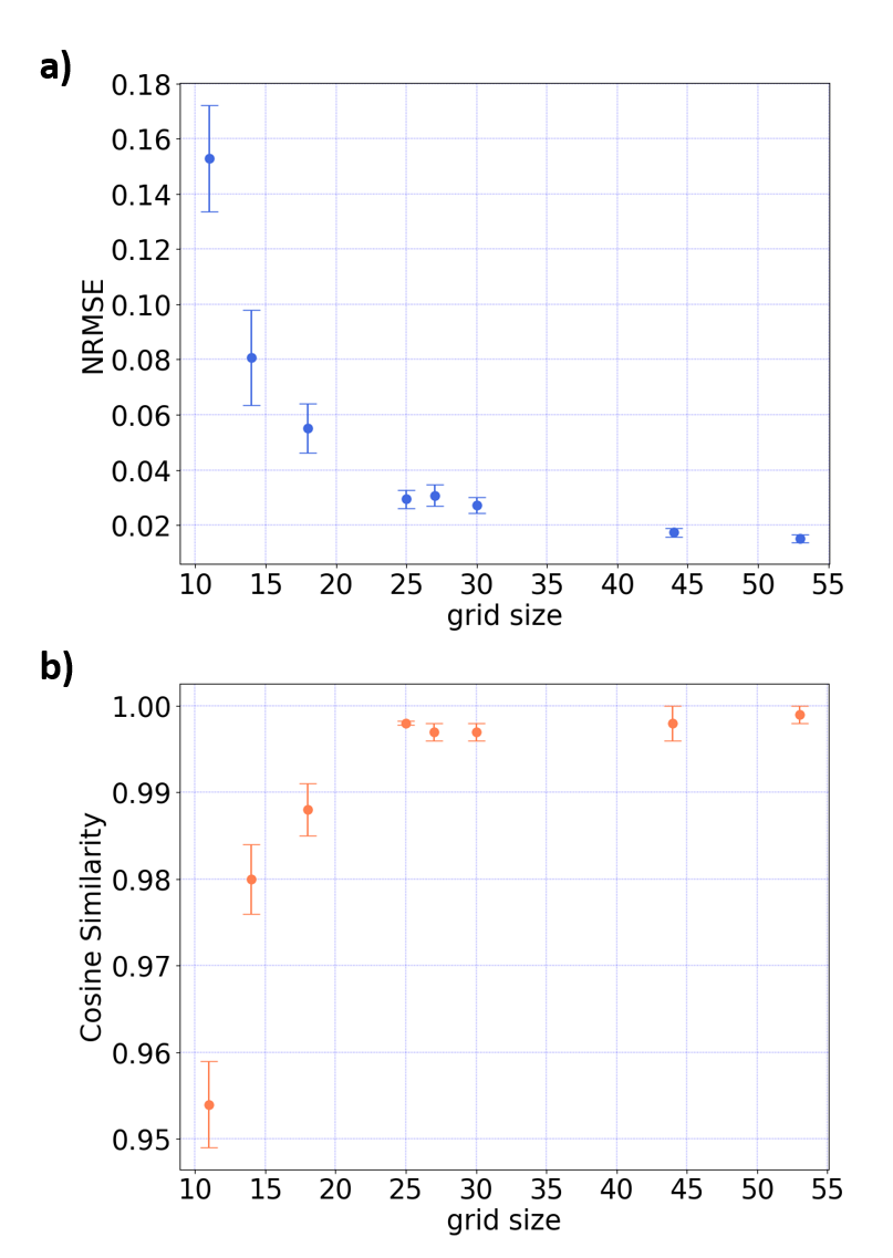
Once established the network architecture, we investigate how the NRMSE on the validation set and the cosine similarity between the network estimation and the true tensions values change reducing the number of tension pairs used for the training. For all the different configurations the size of the training set, and consequently of the validation one, changes depending on the dimension of the tension grid used. Conversely, the number of examples making up the test set remains fixed to . For all the new training configurations the test data are still extracted randomly from the largest grid. This choice is performed to assess how much reducing the data for the training affects the final network estimation of new examples. Figure 3 reports the NRMSE on the validation set, obtained from multiple trainings of the network and the cosine similarity among the network estimation and the expected values in the test set. As expected, the NRMSE achieved by the network decreases as the number of training examples increases, allowing a better reconstruction of the function mapping the input vector onto the output one. A better reconstruction of this function grants higher network performances on the independent test set, as shown by the growth of the cosine similarity between the reconstructed tensions vectors by the NN and the real one. The error on the cosine similarity values gives an indication about the variability linked to the analysis of different examples that randomly fall in different regions of the probabilities functions. In parallel, the error on the NRMSE values depends on the results of different trainings of the algorithm that, starting with random initial parameters, can end up in slightly different conditions.
II.3 Results on experimental data
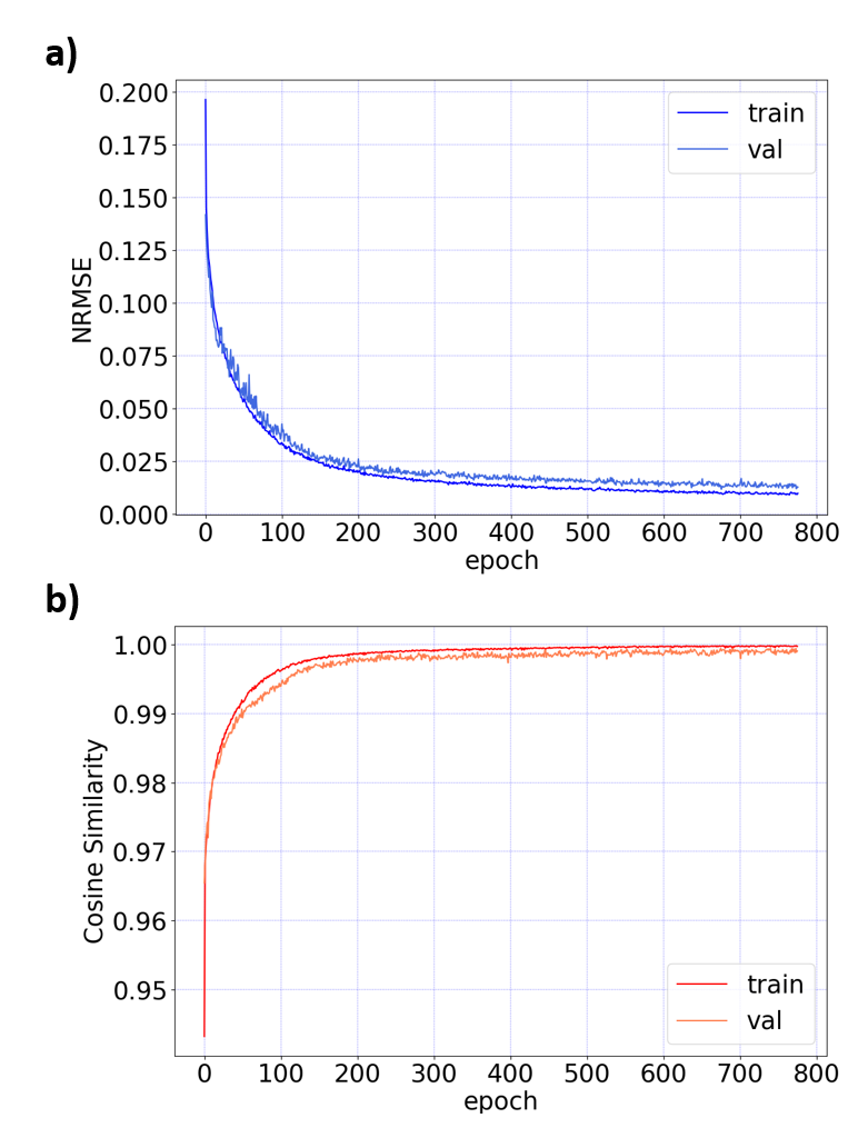
Here, the network architecture resulting from the previous analysis has been implemented and tested training the NN directly on actual experimental data. This is possible thanks to the network efficiency to learn the function which maps the input-output probabilities to the tensions applied. In this way, a good estimate of the tensions values is obtained. If the explicit model Eq. (1) is available, this same procedure is also effective to calibrate the response of the device explicitly in terms of the phases; the exact description of the further propagation and measurement steps is not needed. We use the data obtained from a tensions grid applied on a second integrated device with the same layout, to train the same network as the one described above. The training with such data takes longer to reach the region where the loss function on the validation set stops decreasing. This is shown in Fig. 4, where the NRMSE and the cosine similarity are reported as a function of the training epochs. The network tensions estimations when new data are acquired are reported in Fig. 5, showing the ability of the network to make accurate predictions of the applied voltages.
III Conclusions
We have reported on the application of a NN based algorithm to perform the calibration of integrated devices depending on two parameters. In this investigation we relied on knowledge of a model to identify the most appropriate regime for collecting the training set. However, this is by no means a necessary step in that the use of the NN itself incorporates the same information that would be present in the model. Remarkably, the NN is able to account for spurious effects such as, in our case, cross-talk between thermal actuators, which are otherwise intricate to describe. It can be foreseen however that some basic modelling of the device could be nevertheless beneficial. The successful characterization of two devices based on a single approximate model shows that the NN performance does not heavily depend on the model’s level of detail. In the same vein, some anticipation of the device output, might reveal whether ambiguities may be present in the chosen range of parameters. We have shown that this is easily accounted for by introducing additional data as input to the NN.
This study brings forward machine learning applications in two respects: it goes beyond optimization of the employed resources when these are severely constrained and shows that this characterization method extends beyond the single parameter regime. The obtained results give evidence that NN can provide an effective, robust and reliable tool for the calibration of complex sensors that depend on multiple parameters, with the advantage of requiring no detailed model of their internal operation.
Acknowledgements.
This work is supported by the European Research Council (ERC) Advanced Grant CAPABLE (Composite integrated photonic platform by femtosecond laser micro-machining, Grant Agreement No. 742745), and from the European Union’s Horizon 2020 research and innovation programme under the PHOQUSING project GA no. 899544. I.G. is supported by Ministero dell’Istruzione, dell’Università e della Ricerca Grant of Excellence Departments (ARTICOLO 1, COMMI 314-337 LEGGE 232/2016).References
- Paris (2009) M. G. Paris, International Journal of Quantum Information 7, 125 (2009).
- Giovannetti et al. (2011) V. Giovannetti, S. Lloyd, and L. Maccone, Nature Photonics 5, 222 (2011).
- Pezzé and Smerzi (2014) L. Pezzé and A. Smerzi, in Atom Interferometry, Proceedings of the International School of Physics Enrico Fermi (edited by G. M. Tino and M. A. Kasevich, IOS Press, Amsterdam, 2014) p. 691.
- Pirandola et al. (2018) S. Pirandola, B. R. Bardhan, T. Gehring, C. Weedbrook, and S. Lloyd, Nature Photonics 12, 724 (2018).
- Polino et al. (2020) E. Polino, M. Valeri, N. Spagnolo, and F. Sciarrino, AVS Quantum Science 2, 024703 (2020).
- Gianani et al. (2020) I. Gianani, M. G. Genoni, and M. Barbieri, IEEE J. Sel. Top. Quantum Electron. 5, 6500207 (2020).
- Flamini et al. (2015) F. Flamini, L. Magrini, A. S. Rab, N. Spagnolo, V. D’Ambrosio, P. Mataloni, F. Sciarrino, T. Zandrini, A. Crespi, R. Ramponi, and R. Osellame, Light: Science & Applications 4, e354 (2015).
- Carolan et al. (2015) J. Carolan, C. Harrold, C. Sparrow, E. Martin-Lopez, N. J. Russell, J. W. Silverstone, P. J. Shadbolt, N. Matsuda, M. Oguma, M. Itoh, G. D. Marshall, M. G. Thompson, J. C. F. Matthews, T. Hashimoto, J. L. O’Brien, and A. Laing, Science 349, 711 (2015).
- Harris et al. (2017) N. C. Harris, G. R. Steinbrecher, M. Prabhu, Y. Lahini, J. Mower, D. Bunandar, C. Chen, F. N. C. Wong, T. Baehr-Jones, M. Hochberg, S. Lloyd, and D. Englund, Nature Photonics 11, 447 (2017).
- Taballione et al. (2019) C. Taballione, T. A. W. Wolterink, J. Lugani, A. Eckstein, B. A. Bell, R. Grootjans, I. Visscher, D. Geskus, C. G. H. Roeloffzen, J. J. Renema, I. A. Walmsley, P. W. H. Pinkse, and K.-J. Boller, Optics Express 27, 26842 (2019).
- Ticknor (2013) J. L. Ticknor, Expert Systems with Applications 40, 5501 (2013).
- Enke et al. (2011) D. Enke, M. Grauer, and N. Mehdiyev, Procedia Computer Science 6, 201 (2011), complex adaptive sysytems.
- Ganesan et al. (2010) N. Ganesan, K. Venkatesh, M. Rama, and A. M. Palani, International Journal of Computer Applications 1, 76 (2010).
- Dunjko and Briegel (2018) V. Dunjko and H. J. Briegel, Reports on Progress in Physics 81, 074001 (2018).
- Mehta et al. (2019) P. Mehta, M. Bukov, C.-H. Wang, A. G. Day, C. Richardson, C. K. Fisher, and D. J. Schwab, Physics Reports 810, 1 (2019).
- Carleo et al. (2019) G. Carleo, I. Cirac, K. Cranmer, L. Daudet, M. Schuld, N. Tishby, L. Vogt-Maranto, and L. Zdeborová, Reviews of Modern Physics 91, 045002 (2019).
- Spagnolo et al. (2017) N. Spagnolo, E. Maiorino, C. Vitelli, M. Bentivegna, A. Crespi, R. Ramponi, P. Mataloni, R. Osellame, and F. Sciarrino, Scientific Reports 7, 14316 (2017).
- Carrasquilla et al. (2019) J. Carrasquilla, G. Torlai, R. G. Melko, and L. Aolita, Nature Machine Intelligence 1, 155 (2019).
- Palmieri et al. (2020) A. M. Palmieri, E. Kovlakov, F. Bianchi, D. Yudin, S. Straupe, J. D. Biamonte, and S. Kulik, npj Quantum Information 6, 1 (2020).
- Rocchetto et al. (2019) A. Rocchetto, S. Aaronson, S. Severini, G. Carvacho, D. Poderini, I. Agresti, M. Bentivegna, and F. Sciarrino, Science Advances 5, eaau1946 (2019).
- Arrazola et al. (2019) J. M. Arrazola, T. R. Bromley, J. Izaac, C. R. Myers, K. Brádler, and N. Killoran, Quantum Science and Technology 4, 024004 (2019).
- Giordani et al. (2020) T. Giordani, A. Suprano, E. Polino, F. Acanfora, L. Innocenti, A. Ferraro, M. Paternostro, N. Spagnolo, and F. Sciarrino, Physical Review Letters 124, 160401 (2020).
- Neugebauer et al. (2020) M. Neugebauer, L. Fischer, A. Jäger, S. Czischek, S. Jochim, M. Weidemüller, and M. Gärttner, arXiv preprint arXiv: 2007.16185 (2020).
- Torlai et al. (2019) G. Torlai, B. Timar, E. P. L. van Nieuwenburg, H. Levine, A. Omran, A. Keesling, H. Bernien, M. Greiner, V. Vuletić, M. D. Lukin, R. G. Melko, and M. Endres, Phys. Rev. Lett. 123, 230504 (2019).
- Tiunov et al. (9482) E. S. Tiunov, V. V. T. (Vyborova), A. E. Ulanov, A. I. Lvovsky, and A. K. Fedorov, Optica 7, 448 (ts , doi = 10.1364/OPTICA.389482,).
- Nichols et al. (2019) R. Nichols, L. Mineh, J. Rubio, J. C. Matthews, and P. A. Knott, Quantum Science and Technology 4, 045012 (2019).
- Melnikov et al. (2018) A. A. Melnikov, H. P. Nautrup, M. Krenn, V. Dunjko, M. Tiersch, A. Zeilinger, and H. J. Briegel, Proceedings of the National Academy of Sciences 115, 1221 (2018).
- Krenn et al. (2016) M. Krenn, M. Malik, R. Fickler, R. Lapkiewicz, and A. Zeilinger, Physical Review Letters 116, 090405 (2016).
- O’Driscoll et al. (2019) L. O’Driscoll, R. Nichols, and P. Knott, Quantum Machine Intelligence 1, 5 (2019).
- Sabapathy et al. (2019) K. K. Sabapathy, H. Qi, J. Izaac, and C. Weedbrook, Physical Review A 100, 012326 (2019).
- Krenn et al. (2020) M. Krenn, M. Erhard, and A. Zeilinger, arXiv preprint arXiv:2002.09970 (2020).
- Gao et al. (2020) X. Gao, M. Erhard, A. Zeilinger, and M. Krenn, Physical Review Letters 125, 050501 (2020).
- Agresti et al. (2019) I. Agresti, N. Viggianiello, F. Flamini, N. Spagnolo, A. Crespi, R. Osellame, N. Wiebe, and F. Sciarrino, Physical Review X 9, 011013 (2019).
- Flamini et al. (2019) F. Flamini, N. Spagnolo, and F. Sciarrino, Quantum Science and Technology 4, 024008 (2019).
- Knott (2016) P. A. Knott, New Journal of Physics 18, 073033 (2016).
- Cimini et al. (2020) V. Cimini, M. Barbieri, N. Treps, M. Walschaers, and V. Parigi, arXiv:2003.03343 (2020).
- Gebhart and Bohmann (2020) V. Gebhart and M. Bohmann, Phys. Rev. Research 2, 023150 (2020).
- Hentschel and Sanders (2010) A. Hentschel and B. C. Sanders, Physical Review Letters 104, 063603 (2010).
- Hentschel and Sanders (2011) A. Hentschel and B. C. Sanders, Physical Review Letters 107, 233601 (2011).
- Lovett et al. (2013) N. B. Lovett, C. Crosnier, M. Perarnau-Llobet, and B. C. Sanders, Physical Review Letters 110, 220501 (2013).
- Bonato et al. (2016) C. Bonato, M. S. Blok, H. T. Dinani, D. W. Berry, M. L. Markham, D. J. Twitchen, and R. Hanson, Nature nanotechnology 11, 247 (2016).
- Palittapongarnpim et al. (2017) P. Palittapongarnpim, P. Wittek, E. Zahedinejad, S. Vedaie, and B. C. Sanders, Neurocomputing 268, 116 (2017).
- Liu and Yuan (2017) J. Liu and H. Yuan, Physical Review A 96, 042114 (2017).
- Paesani et al. (2017) S. Paesani, A. A. Gentile, R. Santagati, J. Wang, N. Wiebe, D. P. Tew, J. L. O’Brien, and M. G. Thompson, Phys. Rev. Lett. 118, 100503 (2017).
- Lumino et al. (2018) A. Lumino, E. Polino, A. S. Rab, G. Milani, N. Spagnolo, N. Wiebe, and F. Sciarrino, Physical Review Applied 10, 044033 (2018).
- Palittapongarnpim and Sanders (2019) P. Palittapongarnpim and B. C. Sanders, Physical Review A 100, 012106 (2019).
- Dinani et al. (2019) H. T. Dinani, D. W. Berry, R. Gonzalez, J. R. Maze, and C. Bonato, Physical Review B 99, 125413 (2019).
- Liu et al. (2020) G. Liu, M. Chen, Y.-X. Liu, D. Layden, and P. Cappellaro, Machine Learning: Science and Technology 1, 015003 (2020).
- Peng and Fan (2020) Y. Peng and H. Fan, Physical Review A 101, 022107 (2020).
- Rambhatla et al. (2020) K. Rambhatla, S. E. D’Aurelio, M. Valeri, E. Polino, N. Spagnolo, and F. Sciarrino, Physical Review Research 2, 033078 (2020).
- Valeri et al. (2020) M. Valeri, E. Polino, D. Poderini, I. Gianani, G. Corrielli, A. Crespi, R. Osellame, N. Spagnolo, and F. Sciarrino, arXiv preprint arXiv:2002.01232 (2020).
- Craigie et al. (2020) K. Craigie, E. Gauger, Y. Altmann, and C. Bonato, arXiv preprint arXiv:2008.08891 (2020).
- Nolan et al. (2020) S. P. Nolan, A. Smerzi, and L. Pezzè, arXiv preprint arXiv:2006.02369 (2020).
- Fiderer et al. (2020) L. J. Fiderer, J. Schuff, and D. Braun, arXiv preprint arXiv:2003.02183 (2020).
- Bernstein et al. (2020) L. Bernstein, A. Sludds, R. Hamerly, V. Sze, J. Emer, and D. Englund, arXiv preprint arXiv:2006.13926 (2020).
- Flamini et al. (2020) F. Flamini, A. Hamann, S. Jerbi, L. M. Trenkwalder, H. P. Nautrup, and H. J. Briegel, New Journal of Physics 22, 045002 (2020).
- Cimini et al. (2019) V. Cimini, I. Gianani, N. Spagnolo, F. Leccese, F. Sciarrino, and M. Barbieri, Physical Review Letters 123, 230502 (2019).
- Haykin (2009) S. Haykin, Neural Networks and Learning Machines (Pearson Prentice Hall, 2009).
- Aggarwal (2018) C. C. Aggarwal, Neural Networks and Deep Learning (Springer, 2018) p. 497.
- Gattass and Mazur (2008) R. R. Gattass and E. Mazur, Nature Photonics 2, 219 (2008).
- G. Della Valle and R. Osellame and P. Laporta (2008) G. Della Valle and R. Osellame and P. Laporta, Journal of Optica A: Pure and Applied Optics 11, 013001 (2008).
- Polino et al. (2019) E. Polino, M. Riva, M. Valeri, R. Silvestri, G. Corrielli, A. Crespi, N. Spagnolo, R. Osellame, and F. Sciarrino, Optica 6, 288 (2019).
- Goodfellow et al. (2016) I. Goodfellow, Y. Bengio, and A. Courville, Deep Learning (The MIT Press, 2016).
- Kingma and Ba (2014) D. P. Kingma and J. Ba, arXiv:1412.6980 (2014).