Contrastive and Generative Graph Convolutional Networks for Graph-based Semi-Supervised Learning

Abstract

Graph-based Semi-Supervised Learning (SSL) aims to transfer the labels of a handful of labeled data to the remaining massive unlabeled data via a graph. As one of the most popular graph-based SSL approaches, the recently proposed Graph Convolutional Networks (GCNs) have gained remarkable progress by combining the sound expressiveness of neural networks with graph structure. Nevertheless, the existing graph-based methods do not directly address the core problem of SSL, i.e., the shortage of supervision, and thus their performances are still very limited. To accommodate this issue, a novel GCN-based SSL algorithm is presented in this paper to enrich the supervision signals by utilizing both data similarities and graph structure. Firstly, by designing a semi-supervised contrastive loss, improved node representations can be generated via maximizing the agreement between different views of the same data or the data from the same class. Therefore, the rich unlabeled data and the scarce yet valuable labeled data can jointly provide abundant supervision information for learning discriminative node representations, which helps improve the subsequent classification result. Secondly, the underlying determinative relationship between the data features and input graph topology is extracted as supplementary supervision signals for SSL via using a graph generative loss related to the input features. Intensive experimental results on a variety of real-world datasets firmly verify the effectiveness of our algorithm compared with other state-of-the-art methods.

Introduction

Semi-Supervised Learning (SSL) focuses on utilizing small amounts of labeled data as well as relatively large amounts of unlabeled data for model training (Zhu 2005). Over the past few decades, SSL has attracted increasing research interests and a variety of approaches have been developed (Zhu, Ghahramani, and Lafferty 2003; Joachims 1999), which usually employ cooperative training (Blum and Mitchell 1998), support vector machines (Bennett and Demiriz 1999; Li and Zhou 2010), consistency regularizers (Tarvainen and Valpola 2017; Laine and Aila 2016; Berthelot et al. 2019), and graph-based methods (Zhu, Ghahramani, and Lafferty 2003; Gong et al. 2015; Belkin, Niyogi, and Sindhwani 2006; Kipf and Welling 2017; Ma et al. 2019). Among them, the graph-based SSL algorithms have gained much attention due to its ease of implementation, solid mathematical foundation, and satisfactory performance.

In a graph-based SSL algorithm, all labeled and unlabeled data are represented by graph nodes and their relationships are depicted by graph edges. Then the problem is to transfer the labels of a handful of labeled nodes (i.e., labeled examples) to the remaining massive unlabeled nodes (i.e., unlabeled examples) such that the unlabeled examples can be accurately classified. A popular method is to use graph Laplacian regularization to enforce the similar examples in the feature space to obtain similar label assignments, such as (Belkin, Niyogi, and Sindhwani 2006; Gong et al. 2015; Bühler and Hein 2009). Recently, research attention has been shifted to the learning of proper network embedding to facilitate the label determination (Kipf and Welling 2017; Defferrard, Bresson, and Vandergheynst 2016; Zhou et al. 2019; Veličković et al. 2018; Hu et al. 2019; Yan, Xiong, and Lin 2018), where Graph Convolutional Networks (GCNs) have been demonstrated to outperform traditional graph-based models due to its impressive representation ability (Wu et al. 2020). Concretely, GCNs generalize Convolutional Neural Networks (CNNs) (LeCun, Bengio et al. 1995) to graph-structured data based on the spectral theory, and thus can reconcile the expressive power of graphs in modeling the relationships among data points for representation learning.

Although graph-based SSL methods have achieved noticeable progress in recent years, they do not directly tackle the core problem of SSL, namely the shortage of supervision. One should note that the number of labeled data in SSL problems is usually very limited, which poses a great difficulty for stable network training and thus will probably degrade the performance of GCNs. To accommodate this issue, in this paper, we aim at sufficiently extracting the supervision information carried by the available data themselves for network training, and develop an effective transductive SSL algorithm via using GCNs. That is to say, the goal is to accurately classify the observed unlabeled graph nodes (Zhu 2005; Gong et al. 2016).

Our proposed method is designed to enrich the supervision signals from two aspects, namely data similarities and graph structure. Firstly, considering that the similarities of data points in the feature space provide the natural supervision signals, we propose to use the recently developed contrastive learning (He et al. 2020; Chen et al. 2020) to fully explore such information. Contrastive learning is an active field of self-supervised learning (Doersch, Gupta, and Efros 2015; Gidaris, Singh, and Komodakis 2018), which is able to generate data representations by learning to encode the similarities or dissimilarities among a set of unlabeled examples (Hjelm et al. 2018). The intuition behind is that the rich unlabeled data themselves can be used as supervision signals to help guide the model training. However, unlike the typical unsupervised contrastive learning methods (Hassani and Khasahmadi 2020; Velickovic et al. 2019), SSL problem also contains scarce yet valuable labeled data, so here we design a new semi-supervised contrastive loss, which additionally incorporates class information to improve the contrastive representation learning for node classification tasks. Specifically, we obtain the node representations generated from global and local views respectively, and then employ the semi-supervised contrastive loss to maximizing the agreement between the representations learned from these two views. Secondly, considering that the graph topology itself contains precious information which can be leveraged as supplementary supervision signals for SSL, we utilize a generative term to explicitly model the relationship between graph and node representations. As a result, the originally limited supervision information of labeled data can be further expanded by exploring the knowledge from both data similarities and graph structure, and thus leading to the improved data representations and classification results. Therefore, we term the proposed method as ‘Contrastive GCNs with Graph Generation’ (CG³). In experiments, we demonstrate the contributions of the supervision clues from utilizing contrastive learning and graph structure, and the superiority of our proposed CG³ to other state-of-the-art graph-based SSL methods has also been verified.

Related Work

In this section, we review some representative works on graph-based SSL and contrastive learning, as they are related to this article.

Graph-based Semi-Supervised Learning

Graph-based SSL has been a popular research area in the past two decades. Early graph-based methods are based on the simple assumption that nearby nodes are likely to have the same label. This purpose is usually achieved by the low-dimensional embeddings with Laplacian eigen-maps (Belkin and Niyogi 2004; Belkin, Niyogi, and Sindhwani 2006), spectral kernels (Zhang and Ando 2006), Markov random walks (Szummer and Jaakkola 2002; Zhou et al. 2004; Gong et al. 2014), etc. Another line is based on graph partition, where the cuts should agree with the class information and are placed in low-density regions (Zhu and Ghahramani 2002; Speriosu et al. 2011). In addition, to further improve the learning performance, various techniques are proposed to jointly model the data features and graph structure, such as deep semi-supervised embedding (Weston et al. 2012) and Planetoid (Yang, Cohen, and Salakhudinov 2016) which regularize a supervised classifier with a Laplacian regularizer or an embedding-based regularizer. Recently, a set of graph-based SSL approaches have been proposed to improve the performance of the above-mentioned techniques, including (Calder et al. 2020; Gong, Yang, and Tao 2019; Calder and Slepčev 2019).

Subsequently, inspired by the success of CNNs on grid-structured data, various types of graph convolutional neural networks have been proposed to extend CNNs to graph-structured data and have demonstrated impressive results in SSL (Dehmamy, Barabási, and Yu 2019; Zhang et al. 2019; Xu et al. 2019). Generally, graph convolution can be attributed to the spatial methods directly working on node features and the spectral methods based on convolutions on nodes. In spatial methods, the convolution is defined as a weighted average function over the neighbors of each node which characterizes the impact exerting to the target node from its neighboring nodes, such as GraphSAGE (Hamilton, Ying, and Leskovec 2017), graph attention network (GAT) (Veličković et al. 2018), and the Gaussian induced convolution model (Jiang et al. 2019b). Different from the spatial methods, spectral graph convolution is usually based on eigen-decomposition, where the locality of graph convolution is considered by spectral analysis (Jiang et al. 2019a). Concretely, a general graph convolution framework based on graph Laplacian is first proposed in (Bruna et al. 2014). Afterwards, ChebyNet (Defferrard, Bresson, and Vandergheynst 2016) optimized the method by using Chebyshev polynomial approximation to realize eigenvalue decomposition. Besides, (Kipf and Welling 2017) proposed GCN via using a localized first-order approximation to ChebyNet, which brings about more efficient filtering operations than spectral CNNs. Despite the noticeable achievements of these graph-based semi-supervised methods in recent years, the main concern in SSL, i.e., the shortage of supervision information, has not been directly addressed.

Contrastive Learning

Contrastive learning is a class of self-supervised approaches which trains an encoder to be contrastive between the representations that depict statistical dependencies of interest and those that do not (Velickovic et al. 2019; Chen et al. 2020; Tschannen et al. 2019). In computer vision, a large collection of works (Hadsell, Chopra, and LeCun 2006; He et al. 2020; Tian, Krishnan, and Isola 2019) learn self-supervised representations of images via minimizing the distance between two views of the same image. Analogously, the concept of contrastive learning has also become the central to some popular word-embedding methods, such as word2vec model (Mikolov et al. 2013) which utilizes co-occurring words and negative sampling to learn the word embeddings.

Recently, contrastive methods can be found in several graph representation learning algorithms. For instance, Deep Graph Infomax (DGI) (Velickovic et al. 2019) extends deep Infomax (Hjelm et al. 2018) via learning node representations through contrasting node and graph encodings. Besides, (Hassani and Khasahmadi 2020) learns node-level and graph-level representations by contrasting the different structures of a graph. Apart from this work, a novel framework for unsupervised graph representation learning is proposed in (Zhu et al. 2020) by maximizing the agreement of node representations between two graph views. Although contrastive learning can use the data themselves to provide the supervision information for representation learning, they are not directly applicable to SSL as they fail to incorporate the labeled data which are scarce yet valuable in SSL. In this paper, we devise a semi-supervised contrastive loss function to exploit the supervision signals contained in both the labeled and unlabeled data, which can help learn the discriminative representations for accurate node classification.

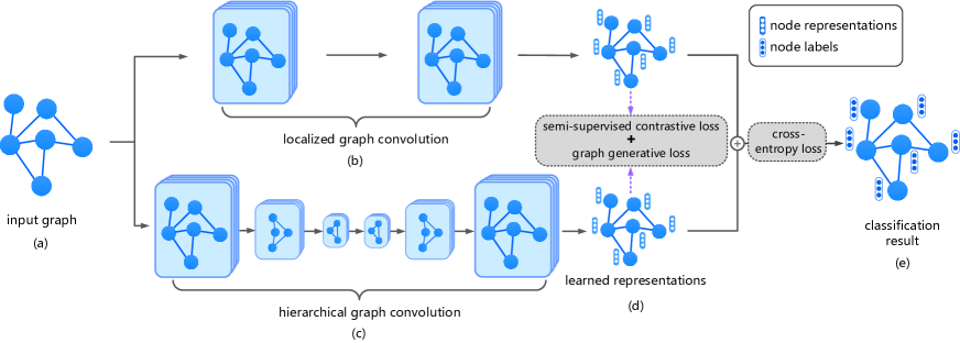
Figure 1: The framework of our approach. In (a), the original graph is adopted as the input of (b) the localized GCNs and (c) the hierarchical GCNs, respectively, where (c) is utilized to capture the global information and serves as the augmented view of (b). In (d), the node representations are generated from (b) and (c), and then constitute the contrastive loss and graph generative loss collaboratively, in order to provide additional supervision signals to improve the representation learning process. In (e), the classification result is acquired via integrating the outputs of (b) and (c), where the cross-entropy loss is used to penalize the difference between the model prediction and the given labels of the initially labeled nodes.

Problem Description

We start by formally introducing the problem of graph-based SSL. Suppose we have a set of $n=l+u$ examples $\Psi=\{\mathbf{x}_{1},\cdots,\mathbf{x}_{l},\mathbf{x}_{l+1},\cdots,\mathbf{x}_{n}\}$, where the first $l$ examples constitute the labeled set with the labels $\{y_{i}\}_{i=1}^{l}$ and the remaining $u$ examples form the unlabeled set with typically $l\ll u$. We denote $\mathbf{X}\in\mathbb{R}^{n\times d}$ as the feature matrix with the $i$-th row formed by the feature vector $\mathbf{x}_{i}$ of the $i$-th example, and $\mathbf{Y}\in\mathbb{R}^{n\times c}$ as the label matrix with its $(i,j)$-th element $\mathbf{Y}_{ij}=1$ if $\mathbf{x}_{i}$ belongs to the $j$-th class and $\mathbf{Y}_{ij}=0$ otherwise. Here $d$ is the feature dimension and $c$ is the number of classes. The dataset $\Phi$ is represented by a graph $\mathcal{G}=\left\langle{\mathcal{V},\mathcal{E}}\right\rangle$, where $\mathcal{V}$ is the node set containing all examples and $\mathcal{E}$ is the edge set modeling the similarity among the nodes/examples. The adjacency matrix of $\mathcal{G}$ is denoted as $\mathbf{A}$ with $\mathbf{A}_{ij}=1$ if there exists an edge between $\mathbf{x}_{i}$ and $\mathbf{x}_{j}$ and $\mathbf{A}_{ij}=0$ otherwise. In this paper, we target transductive graph-based SSL which aims to find the labels $y_{l+1},y_{l+2},\cdots,y_{n}$ of the unlabeled examples $\mathbf{x}_{l+1},\mathbf{x}_{l+2},\cdots,\mathbf{x}_{n}$ based on $\Psi$.

Method

This section details our proposed CG³ model (see Figure 1). Specifically, we illustrate the critical components of CG³ by explaining the multi-view establishment for graph convolutions, presenting the semi-supervised contrastive learning, elaborating the graph generative loss, and describing the overall training procedure.

Multi-View Establishment for Graph Convolutions

In our CG³ method, we need to firstly build two different views for the subsequent graph contrastive learning. Note that in self-supervised visual representation learning tasks, contrasting congruent and incongruent views of images enables the algorithms to learn expressive representations (Tian, Krishnan, and Isola 2019; He et al. 2020). However, unlike the regular grid-like image data where different views can be simply generated by standard augmentation techniques such as cropping, rotation, or color distortion, the view augmentation on irregular graph data is not trivial, as graph nodes and edges do not contain visually semantic contents as in the image (Velickovic et al. 2019). Although edge removing or adding is a simple way to generate a related graph, it might damage the original graph topology, and thus degrading the representation results of graph convolutions. Instead of directly changing the graph structure, we employ two types of graph convolutions to generate node representations from two different views revealing the local and global cues. In this means, the representations generated by different views complement to each other and thus enriching the final representation results. Specifically, by performing contrastive learning between the obtained representations from two views, the rich global and local information can be encoded simultaneously. This process will be detailed as follows.

To obtain node representations from the local view, we actually have many choices of network architectures, such as the commonly-used GCN (Kipf and Welling 2017) and GAT (Veličković et al. 2018) which produce node representations by aggregating neighborhood information. For simplicity, we adopt the GCN model (Kipf and Welling 2017) as our backbone in the local view. In this work, a two-layer GCN is employed with the input feature matrix $\mathbf{X}$ and adjacency matrix $\mathbf{A}$, namely

$$\mathbf{H}^{\phi_{1}}=\hat{\mathbf{A}}\sigma(\hat{\mathbf{A}}\mathbf{X}{\mathbf{W}^{(0)}}){\mathbf{W}^{(1)}},$$ (1)

where $\hat{\mathbf{A}}={\tilde{\mathbf{D}}^{-\frac{1}{2}}}\tilde{\mathbf{A}}{\tilde{\mathbf{D}}^{-\frac{1}{2}}}$, $\tilde{\mathbf{A}}=\mathbf{A}+\mathbf{I}$, ${\tilde{\mathbf{D}}_{ii}}=\sum\nolimits_{j}{{{\tilde{\mathbf{A}}}_{ij}}}$, $\mathbf{W}^{(0)}$ and $\mathbf{W}^{(1)}$ denote the trainable weight matrices, $\sigma(\cdot)$ represents an activation function (e.g., the ReLU function (Nair and Hinton 2010)), and $\mathbf{H}^{\phi_{1}}$ denotes the representation result learned from view $\phi_{1}$ (i.e., the local view).

Afterwards, we employ a simple yet effective hierarchical GCN model, i.e., HGCN (Hu et al. 2019), to generate the representations from the global view. Concretely, HGCN repeatedly aggregates the structurally similar graph nodes to a set of hyper-nodes, which can produce coarsened graphs for convolution and enlarge the receptive field for the nodes. Then, the symmetric graph refining layers are applied to restore the original graph structure for node-level representation learning. Such a hierarchical graph convolution model comprehensively captures the nodes’ information from local to global perspectives. As a result, the representations $\mathbf{H}^{\phi_{2}}$ can be generated from the global view (i.e., view $\phi_{2}$), which provides complementary information to $\mathbf{H}^{\phi_{1}}$.

Semi-Supervised Contrastive Learning

Unsupervised contrastive methods have led to great success in various domains, as they can exploit rich information contained in the data themselves to guide the representation learning process. However, the unsupervised contrastive techniques (Hassani and Khasahmadi 2020; Zhu et al. 2020) fail to explore the class information which is scarce yet valuable in SSL problems. To address this issue, we propose a semi-supervised contrastive loss which incorporates the class information to improve the contrastive representation learning. The proposed semi-supervised contrastive loss can be partitioned into two parts, namely the supervised and unsupervised contrastive losses.

Formally, the unsupervised contrastive learning is expected to achieve the effect as

$${\rm{score}}(f({\mathbf{x}_{i}}),f(\mathbf{x}_{i}^{+}))\gg{\rm{score}}(f({\mathbf{x}_{i}}),f(\mathbf{x}_{i}^{-})),$$ (2)

where $\mathbf{x}_{i}^{+}$ is a node similar or congruent to $\mathbf{x}_{i}$, $\mathbf{x}_{i}^{-}$ is a node dissimilar to $\mathbf{x}_{i}$, $f$ is an encoder, and the score function is used to measure the similarity of encoded features of two nodes. Here, ($\mathbf{x}_{i}$, $\mathbf{x}_{i}^{+}$) and ($\mathbf{x}_{i}$, $\mathbf{x}_{i}^{-}$) indicate the positive and negative pairs, respectively. Eq. (2) encourages the score function to assign large values to the positive pairs and small values to the negative pairs, which can be used as the supervision signals to guide the learning process of encoder $f$. By resorting to the above-mentioned explanations, our unsupervised contrastive loss ${\mathcal{L}_{uc}}$ can be presented as

$${\mathcal{L}_{uc}}=\frac{1}{{2n}}\sum\limits_{i=1}^{n}{(\mathcal{L}_{uc}^{\phi_{1}}({\mathbf{x}_{i}})+\mathcal{L}_{uc}^{\phi_{2}}({\mathbf{x}_{i}}))},$$ (3)

where $\mathcal{L}_{uc}^{\phi_{1}}({\mathbf{x}_{i}})$ and $\mathcal{L}_{uc}^{\phi_{2}}({\mathbf{x}_{i}})$ denote the unsupervised pairwise contrastive losses of $\mathbf{x}_{i}$ in local and global views, respectively. Further, $\mathcal{L}_{uc}^{\phi_{1}}({\mathbf{x}_{i}})$ can be obtained with the similarity measured by inner product, namely

$${\mathcal{L}_{uc}^{{\phi_{1}}}}({\mathbf{x}_{i}})=-\log\frac{{\exp(\langle\mathbf{h}_{i}^{{\phi_{1}}},\mathbf{h}_{i}^{{\phi_{2}}}\rangle)}}{{\sum\nolimits_{j=1}^{n}{\exp(\langle\mathbf{h}_{i}^{{\phi_{1}}},\mathbf{h}_{j}^{{\phi_{2}}}\rangle)}}},$$ (4)

where $\mathbf{h}_{i}^{\phi_{1}}=\mathbf{H}_{i,:}^{\phi_{1}}$ and $\mathbf{h}_{i}^{\phi_{2}}=\mathbf{H}_{i,:}^{\phi_{2}}$ denote the representation results of $\mathbf{x}_{i}$ learned from the local and global views, respectively, and $\langle\cdot\rangle$ denotes the inner product. Here $\mathbf{H}^{\phi_{v}}_{i,:}$ denotes the $i$-th row of the matrix $\mathbf{H}^{\phi_{v}}$ for $v=1,2$. By using Eq. (4), the similarity of the positive pairs (i.e., $\mathbf{h}_{i}^{{\phi_{1}}}$ and $\mathbf{h}_{i}^{{\phi_{2}}}$) can be contrasted with that of the negative pairs, and then $\mathcal{L}_{uc}^{\phi_{2}}({\mathbf{x}_{i}})$ can be similarly calculated by

$${\mathcal{L}_{uc}^{{\phi_{2}}}}({\mathbf{x}_{i}})=-\log\frac{{\exp(\langle\mathbf{h}_{i}^{{\phi_{2}}},\mathbf{h}_{i}^{{\phi_{1}}}\rangle)}}{{\sum\nolimits_{j=1}^{n}{\exp(\langle\mathbf{h}_{i}^{{\phi_{2}}},\mathbf{h}_{j}^{{\phi_{1}}}\rangle)}}}.$$ (5)

To incorporate the scarce yet valuable class information for model training, we propose to use a supervised contrastive loss as follows:

$${\mathcal{L}_{sc}}=\frac{1}{{2l}}\sum\limits_{i=1}^{l}{(\mathcal{L}_{sc}^{{\phi_{1}}}({\mathbf{x}_{i}})+\mathcal{L}_{sc}^{{\phi_{2}}}({\mathbf{x}_{i}}))}.$$ (6)

Here, the supervised pairwise contrastive loss of $\mathbf{x}_{i}$ can be computed as

$$\mathcal{L}_{sc}^{{\phi_{1}}}({\mathbf{x}_{i}})=-\log\frac{{\sum\nolimits_{k=1}^{l}{{\mathbbm{1}_{[{y_{i}}={y_{k}}]}}\exp(\langle\mathbf{h}_{i}^{{\phi_{1}}},\mathbf{h}_{k}^{{\phi_{2}}}\rangle)}}}{{\sum\nolimits_{j=1}^{l}{\exp(\langle\mathbf{h}_{i}^{{\phi_{1}}},\mathbf{h}_{j}^{{\phi_{2}}}\rangle)}}},$$ (7)

$$\mathcal{L}_{sc}^{{\phi_{2}}}({\mathbf{x}_{i}})=-\log\frac{{\sum\nolimits_{k=1}^{l}{{\mathbbm{1}_{[{y_{i}}={y_{k}}]}}\exp(\langle\mathbf{h}_{i}^{{\phi_{2}}},\mathbf{h}_{k}^{{\phi_{1}}}\rangle)}}}{{\sum\nolimits_{j=1}^{l}{\exp(\langle\mathbf{h}_{i}^{{\phi_{2}}},\mathbf{h}_{j}^{{\phi_{1}}}\rangle)}}},$$ (8)

where ${\mathbbm{1}_{[\cdot]}}$ is an indicator function which equals to 1 if the argument inside the bracket holds, and 0 otherwise. Different from the unsupervised contrastive learning in Eqs. (4) and (5), here the positive and negative pairs are constructed based on the facts that whether two nodes belong to the same class. In other words, a data pair is positive if both examples have the same label, and is negative if their labels are different.

By combining the supervised and unsupervised contrastive losses, we arrive at the following semi-supervised contrastive loss:

$${\mathcal{L}_{ssc}}={\mathcal{L}_{uc}}+{\mathcal{L}_{sc}}.$$ (9)

The mechanism of our semi-supervised contrastive learning has been exhibited in Figure 2. By minimizing ${\mathcal{L}_{ssc}}$, the rich unlabeled data and the scarce yet valuable labeled data work collaboratively to provide additional supervision signals for discriminative representation learning, which can further improve the subsequent classification result.

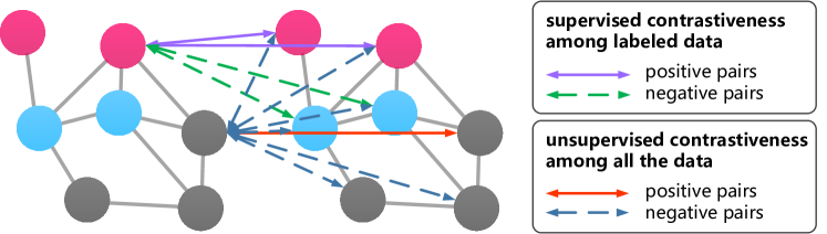
Figure 2: The mechanism of our semi-supervised contrastive learning. The red and blue circles denote the labeled graph nodes, where each color corresponds to a specific class, and the gray circles represent the unlabeled graph nodes. Various contrastive strategies adopted by our method are illustrated by the arrows with different colors and line styles.

Graph Generative Loss

Apart from the supervision information extracted from data similarities via contrastive learning, we also intend to distill the graph topological information to better guide the representation learning process. In this work, a graph generative loss is utilized to encode the graph structure and model the underlying relationship between the feature representations and graph topology. Inspired by the generative models (Hoff, Raftery, and Handcock 2002; Kipf and Welling 2016; Ma et al. 2019), we let the graph edge $e_{ij}$ be the binary random variable with $e_{ij}=1$ indicating the existence of the edge between $\mathbf{x}_{i}$ and $\mathbf{x}_{j}$, and $e_{ij}=0$ otherwise. Here the edges are assumed to be conditionally independent, so that the conditional probability of the input graph $\mathcal{G}$ given $\mathbf{H}^{\phi_{1}}$ and $\mathbf{H}^{\phi_{2}}$ can be factorized as

$${p}(\mathcal{G}|\mathbf{H}^{\phi_{1}},\mathbf{H}^{\phi_{2}})=\prod\limits_{i,j}{{p}({e_{ij}}|\mathbf{H}^{\phi_{1}},\mathbf{H}^{\phi_{2}})}.$$ (10)

Similar to the latent space models (Hoff, Raftery, and Handcock 2002; Ma et al. 2019), we reasonably assume that the probability of $e_{ij}$ only depends on the representations of $\mathbf{x}_{i}$ and $\mathbf{x}_{j}$. Meanwhile, to further maximize the node-level agreement across the global and local views, the conditional probability of $e_{ij}$ can be obtained as ${{p}({e_{ij}}|\mathbf{H}^{\phi_{1}},\mathbf{H}^{\phi_{2}})}={{p}({e_{ij}}|\mathbf{h}_{i}^{\phi_{1}},\mathbf{h}_{j}^{\phi_{2}})}$. Finally, for practical use, we specify the parametric forms of the conditional probability by using a logit model, which arrives at

$${p}(\mathcal{G}|\mathbf{H}^{\phi_{1}},\mathbf{H}^{\phi_{2}})=\prod\limits_{i,j}{{p}({e_{ij}}|\mathbf{h}_{i}^{\phi_{1}},\mathbf{h}_{j}^{\phi_{2}})}=\prod\limits_{i,j}\delta([\mathbf{h}_{i}^{{\phi_{1}}},\mathbf{h}_{j}^{{\phi_{2}}}]\mathbf{w}),$$ (11)

where $\delta(\cdot)$ is the logistic function, $\mathbf{w}$ is the learnable parameter vector, and $[\cdot,\cdot]$ is the concatenation operation. By maximizing Eq. (11), the observed graph structure can be taken into consideration along with data feature and scarce label information for node classification, and thus the graph generative loss can be formulated as $\mathcal{L}_{g^{2}}=-{p}(\mathcal{G}|\mathbf{H}^{\phi_{1}},\mathbf{H}^{\phi_{2}})$.

Model Training

To obtain the overall network output $\mathbf{O}$, we integrate the representation results generated by the GCN and HGCN models, so that the rich information from both local and global views can be exploited, which is expressed as

$$\mathbf{O}=\lambda^{\phi_{1}}\mathbf{H}^{\phi_{1}}+(1-\lambda^{\phi_{1}})\mathbf{H}^{\phi_{2}},$$ (12)

where $0<\lambda^{\phi_{1}}<1$ is the weight assigned to $\mathbf{H}^{\phi_{1}}$. Afterwards, the cross-entropy loss can be adopted to penalize the differences between the network output $\mathbf{O}$ and the labels of the originally labeled nodes as

$${\mathcal{L}_{ce}}=-\sum\limits_{i=1}^{l}{\sum\limits_{j=1}^{c}{{\mathbf{Y}_{ij}}\ln{\mathbf{O}_{ij}}}}.$$ (13)

Finally, by combining $\mathcal{L}_{ce}$ with the semi-supervised contrastive loss $\mathcal{L}_{ssc}$ and the graph generative loss $\mathcal{L}_{g^{2}}$, the overall loss function of our CG³ can be presented as

$$\mathcal{L}={\mathcal{L}_{ce}}+\lambda_{ssc}{\mathcal{L}_{ssc}}+\lambda_{g^{2}}{\mathcal{L}_{g^{2}}},$$ (14)

where $\lambda_{ssc}>0$ and $\lambda_{g^{2}}>0$ are tuning parameters to weight the importance of $\mathcal{L}_{ssc}$ and $\mathcal{L}_{g^{2}}$, respectively. The detailed description of our CG³ is provided in Algorithm 1.

Algorithm 1 The Proposed CG³ algorithm

1:Feature matrix $\mathbf{X}$; adjacency matrix $\mathbf{A}$; label matrix $\mathbf{Y}$; maximum number of iterations $\mathcal{T}$

2:for $t=1$ to $\mathcal{T}$ do

3:     // Multi-view representation learning

4:     Perform localized graph convolution (i.e., Eq. (1)) and hierarchical graph convolution (Hu et al. 2019) to obtain $\mathbf{H}^{\phi_{1}}$ and $\mathbf{H}^{\phi_{2}}$, respectively;

5:     // Calculate loss values

6:     Calculate semi-supervised contrastive loss ${\mathcal{L}_{ssc}}$ based on Eqs. (3) and (6);

7:     Calculate the graph generative loss ${\mathcal{L}_{g^{2}}}$ based on Eq. (11);

8:     Calculate the cross-entropy loss ${\mathcal{L}_{ce}}$ with Eq. (13);

9:     Update the network parameters according to the overall loss function $\mathcal{L}$ in Eq. (14);

10:end for

11:Conduct label prediction based on the trained network;

12:Predicted label for each unlabeled graph node.

Table 1: Dataset statistics

Datasets	Nodes	Edges	Features	Classes
Cora	2,708	5,429	1,433	7
CiteSeer	3,327	4,732	3,703	6
PubMed	19,717	44,338	500	3
Amazon Computers	13,752	245,861	767	10
Amazon Photo	7,650	119,081	745	8
Coauthor CS	18,333	81,894	6,805	15

Experimental Results

To demonstrate the effectiveness of our proposed CG³ method, extensive experiments have been conducted on six benchmark datasets including three widely-used citation networks (i.e., Cora, CiteSeer, and PubMed) (Sen et al. 2008; Bojchevski and Günnemann 2018), two Amazon product co-purchase networks (i.e., Amazon Computers and Amazon Photo) (Shchur et al. 2018), and one co-author network subjected to computer science (i.e., Coauthor CS) (Shchur et al. 2018). Dataset statistics are summarized in Table 1. We report the mean accuracy of ten independent runs for every algorithm on each dataset to achieve fair comparison.

Table 2: Classification accuracies of compared methods on Cora, CiteSeer, PubMed, Amazon Computers, Amazon Photo, and Coauthor CS datasets. Some records are not associated with standard deviations as they are directly taken from (Hassani and Khasahmadi 2020) which did not report standard deviations.

Method	Cora	CiteSeer	PubMed	Amazon Computers	Amazon Photo	Coauthor CS
LP	68.0	45.3	63.0	70.8$\pm$0.0	67.8$\pm$0.0	74.3$\pm$0.0
Chebyshev	81.2	69.8	74.4	62.6$\pm$0.0	74.3$\pm$0.0	91.5$\pm$0.0
GCN	81.5	70.3	79.0	76.3$\pm$0.5	87.3$\pm$1.0	91.8$\pm$0.1
GAT	83.0$\pm$0.7	72.5$\pm$0.7	79.0$\pm$0.3	79.3$\pm$1.1	86.2$\pm$1.5	90.5$\pm$0.7
SGC	81.0$\pm$0.0	71.9$\pm$0.1	78.9$\pm$0.0	74.4$\pm$0.1	86.4$\pm$0.0	91.0$\pm$0.0
DGI	81.7$\pm$0.6	71.5$\pm$0.7	77.3$\pm$0.6	75.9$\pm$0.6	83.1$\pm$0.5	90.0$\pm$0.3
GMI	82.7$\pm$0.2	73.0$\pm$0.3	80.1$\pm$0.2	76.8$\pm$0.1	85.1$\pm$0.1	91.0$\pm$0.0
MVGRL	82.9$\pm$0.7	72.6$\pm$0.7	79.4$\pm$0.3	79.0$\pm$0.6	87.3$\pm$0.3	91.3$\pm$0.1
GRACE	80.0$\pm$0.4	71.7$\pm$0.6	79.5$\pm$1.1	71.8$\pm$0.4	81.8$\pm$1.0	90.1$\pm$0.8
CG3	83.4$\pm$0.7	73.6$\pm$0.8	80.2$\pm$0.8	79.9$\pm$0.6	89.4$\pm$0.5	92.3$\pm$0.2

Node Classification Results

We evaluate the performance of our proposed CG³ method on transductive semi-supervised node classification tasks by comparing it with a variety of methods, including Label Propagation (LP) (Zhu, Ghahramani, and Lafferty 2003), Chebyshev (Defferrard, Bresson, and Vandergheynst 2016), GCN (Kipf and Welling 2017), GAT (Veličković et al. 2018), SGC (Wu et al. 2019), DGI (Velickovic et al. 2019), GMI (Peng et al. 2020), MVGRL (Hassani and Khasahmadi 2020), and GRACE (Zhu et al. 2020). For the widely-used Cora, CiteSeer, and PubMed datasets, we use the same train/validation/test splits as (Yang, Cohen, and Salakhudinov 2016). For the other three datasets (i.e., Amazon Computers, Amazon Photo, and Coauthor CS), we use 30 labeled nodes per class as the training set, 30 nodes per class as the validation set, and the rest as the test set. Note that the selection of labeled nodes on each dataset is kept identical for all compared methods.

Classification results are reported in Table 2, where the highest record on each dataset has been highlighted in bold. Notably, the GCN-based contrastive models (i.e., DGI, GMI, MVGRL, GRACE, and CG³) can generally achieve strong performance across all six datasets, which is due to the reason that contrastive learning aims to extract additional supervision information from data similarities for improving the learned representations, and thus obtaining promising classification results. In our CG³, two different types of GCNs are adopted to aggregate information from both local and global views. Meanwhile, CG³ enriches the supervision signals from data similarities and graph structure simultaneously, which can help generate discriminative representations for classification tasks. Consequently, the proposed CG³ consistently surpasses other contrastive methods and achieves the top level performance among all baselines on these six datasets.

Table 3: Classification accuracies with different label rates on Cora dataset.

Label Rate	0.5%	1%	2%	3%
LP	56.4	62.3	65.4	67.5
Chebyshev	36.4	54.7	55.5	67.3
GCN	42.6	56.9	67.8	74.9
GAT	56.4	71.7	73.5	78.5
SGC	43.7	64.3	68.9	71.0
DGI	67.5	72.4	75.6	78.9
GMI	67.1	71.0	76.1	78.8
MVGRL	61.6	65.2	74.7	79.0
GRACE	60.4	70.2	73.0	75.8
CG3	69.3	74.1	76.6	79.9

Results under Scarce Labeled Training Data

To further investigate the ability of our proposed CG³ in dealing with scarce supervision, we conduct experiments when the number of labeled examples is extremely small. For each run, we follow (Li, Han, and Wu 2018) and select a small set of labeled examples for model training. The specific label rates are 0.5%, 1%, 2%, 3% for Cora and CiteSeer datasets, and 0.03%, 0.05%, 0.1% for PubMed dataset. Here, the baselines are kept identical with the previous node classification experiments.

The results shown in Tables 3, 4, and 5 again verify the effectiveness of our CG³ method. We see that CG³ outperforms other state-of-the-art approaches under different small label rates across the three datasets. It can be observed that the performance of GCN significantly declines when the label information is very limited (e.g., at the label rate of 0.5% on Cora dataset) due to the inefficient propagation of label information. In contrast, the GCN-based contrastive models (i.e., DGI, GMI, MVGRL, GRACE, and CG³) can often achieve much better results with few labeled data, which demonstrates the benefits of extracting supervision information from data themselves to learn powerful representations for classification tasks. Besides, it is noteworthy that on each dataset, our CG³ consistently outperforms the other GCN-based contrastive approaches (i.e., DGI, GMI, MVGRL, and GRACE) by a large margin, especially when the labeled data becomes very limited. This is due to that our proposed CG³ can additionally exploit the supervision signals from graph topological and label information simultaneously, which has often been ignored by other contrastive models.

Table 4: Classification accuracies with different label rates on CiteSeer dataset.

Label Rate	0.5%	1%	2%	3%
LP	34.8	40.2	43.6	45.3
Chebyshev	19.7	59.3	62.1	66.8
GCN	33.4	46.5	62.6	66.9
GAT	45.7	64.7	69.0	69.3
SGC	43.2	50.7	55.8	60.9
DGI	60.7	66.9	68.1	69.8
GMI	56.2	63.5	65.7	68.0
MVGRL	61.7	66.6	68.5	70.3
GRACE	55.4	59.3	63.4	67.8
CG3	62.7	70.6	70.9	71.3

Table 5: Classification accuracies with different label rates on PubMed dataset.

Label Rate	0.03%	0.05%	0.1%
LP	61.4	65.4	66.4
Chebyshev	55.9	62.5	69.5
GCN	61.8	68.8	71.9
GAT	65.7	69.9	72.4
SGC	62.5	69.4	69.9
DGI	60.2	68.4	70.7
GMI	60.1	62.4	71.4
MVGRL	63.3	69.4	72.2
GRACE	64.4	67.5	72.3
CG3	68.3	70.1	73.2

Table 6: Ablation study of the contrastive and generative losses on Cora, CiteSeer, and PubMed datasets.

Method	Cora	CiteSeer	PubMed
CG3 (w/o ConLoss)	79.2$\pm$0.7	69.8$\pm$1.3	76.6$\pm$1.0
CG3 (w/o GenLoss)	82.9$\pm$0.9	72.9$\pm$0.9	79.8$\pm$0.9
CG3	83.4$\pm$0.7	73.6$\pm$0.8	80.2$\pm$0.8

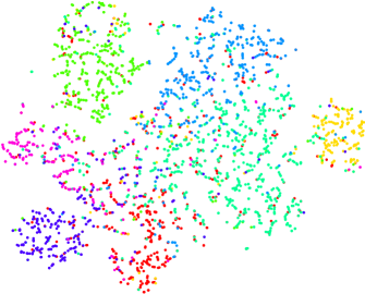
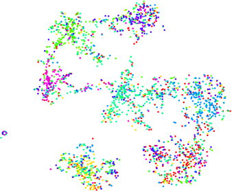
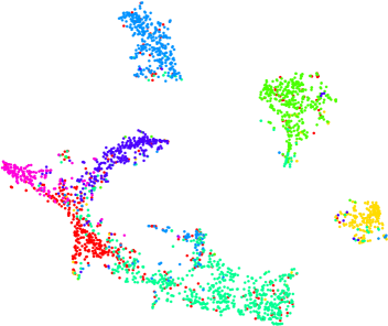
Figure 3: t-SNE embeddings of the nodes acquired by different methods on Cora dataset. (a) GCN; (b) HGCN; (c) CG³.

Ablation Study

As is mentioned in the introduction, our proposed CG³ employs the contrastive and graph generative losses to enrich the supervision signals from the data similarities and graph structure, respectively. To shed light on the contributions of these two components, we report the classification results of CG³ when each of the two components is removed on the three previously-used datasets including Cora, CiteSeer, and PubMed. The data splits are kept identical with (Yang, Cohen, and Salakhudinov 2016). For simplicity, we adopt ‘CG³ (w/o ConLoss)’ and ‘CG³ (w/o GenLoss)’ to represent the reduced models by removing the contrastive loss $\mathcal{L}_{ssc}$ and the graph generative loss $\mathcal{L}_{g^{2}}$, respectively, and the comparative results have been exhibited in Table 6. It is apparent that the classification accuracy will decrease when any one of the aforementioned components is dropped, which reveals that both components make essential contributions to boosting the performance. In particular, our proposed model is able to improve the classification performance substantially by utilizing the contrastive loss, e.g., the accuracy can be raised by nearly 4% on CiteSeer dataset.

Meanwhile, it is noteworthy that our proposed model performs graph convolution in different views based on two parallel networks (i.e., GCN and HGCN), and also conducts contrastive operation between these two views. As a result, the abundant local and global information are encoded simultaneously to obtain the improved data representations for classification. To reveal this, we visualize the embedding results of Cora dataset generated by GCN, HGCN, and CG³ via using t-SNE method (Maaten and Hinton 2008), which are given in Figure 3. As can be observed, the 2D projections of the embeddings generated by our CG³ (see Figure 3) can exhibit more coherent clusters when compared with the other two methods. Therefore, we believe that the contrastiveness among multi-view graph convolutions is beneficial to rendering promising classification results.

Conclusion

In this paper, we have presented the Contrastive GCNs with Graph Generation (CG³) which is a new GCN-based approach for transductive semi-supervised node classification. By designing a semi-supervised contrastive loss, the scarce yet valuable class information, together with the data similarities, can be used to provide abundant supervision information for discriminative representation learning. Moreover, the supervision signals can be further enriched by leveraging the underlying relationship between the input graph topology and data features. Experiments on various public datasets illustrate the effectiveness of our method in solving different kinds of node classification tasks.

References

- Belkin and Niyogi (2004) Belkin, M.; and Niyogi, P. 2004. Semi-supervised learning on Riemannian manifolds. Machine learning 56: 209–239.
- Belkin, Niyogi, and Sindhwani (2006) Belkin, M.; Niyogi, P.; and Sindhwani, V. 2006. Manifold regularization: A geometric framework for learning from labeled and unlabeled examples. Journal of machine learning research 7: 2399–2434.
- Bennett and Demiriz (1999) Bennett, K. P.; and Demiriz, A. 1999. Semi-supervised support vector machines. In NeurIPS, 368–374.
- Berthelot et al. (2019) Berthelot, D.; Carlini, N.; Goodfellow, I.; Papernot, N.; Oliver, A.; and Raffel, C. A. 2019. Mixmatch: A holistic approach to semi-supervised learning. In NeurIPS, 5049–5059.
- Blum and Mitchell (1998) Blum, A.; and Mitchell, T. 1998. Combining labeled and unlabeled data with co-training. In COLT, 92–100.
- Bojchevski and Günnemann (2018) Bojchevski, A.; and Günnemann, S. 2018. Deep gaussian embedding of graphs: Unsupervised inductive learning via ranking. In ICLR.
- Bruna et al. (2014) Bruna, J.; Zaremba, W.; Szlam, A.; and LeCun, Y. 2014. Spectral networks and locally connected networks on graphs. In ICLR.
- Bühler and Hein (2009) Bühler, T.; and Hein, M. 2009. Spectral clustering based on the graph p-Laplacian. In ICML, 81–88.
- Calder et al. (2020) Calder, J.; Cook, B.; Thorpe, M.; and Slepcev, D. 2020. Poisson Learning: Graph based semi-supervised learning at very low label rates. Proceedings of machine learning research 119.
- Calder and Slepčev (2019) Calder, J.; and Slepčev, D. 2019. Properly-weighted graph Laplacian for semi-supervised learning. Applied mathematics & optimization 1–49.
- Chen et al. (2020) Chen, T.; Kornblith, S.; Norouzi, M.; and Hinton, G. 2020. A simple framework for contrastive learning of visual representations. arXiv preprint arXiv:2002.05709 .
- Defferrard, Bresson, and Vandergheynst (2016) Defferrard, M.; Bresson, X.; and Vandergheynst, P. 2016. Convolutional neural networks on graphs with fast localized spectral filtering. In NeurIPS, 3844–3852.
- Dehmamy, Barabási, and Yu (2019) Dehmamy, N.; Barabási, A.-L.; and Yu, R. 2019. Understanding the representation power of graph neural networks in learning graph topology. In NeurIPS, 15413–15423.
- Doersch, Gupta, and Efros (2015) Doersch, C.; Gupta, A.; and Efros, A. A. 2015. Unsupervised visual representation learning by context prediction. In ICCV, 1422–1430.
- Gidaris, Singh, and Komodakis (2018) Gidaris, S.; Singh, P.; and Komodakis, N. 2018. Unsupervised representation learning by predicting image rotations. In ICLR.
- Gong et al. (2015) Gong, C.; Liu, T.; Tao, D.; Fu, K.; Tu, E.; and Yang, J. 2015. Deformed graph Laplacian for semisupervised learning. IEEE transactions on neural networks and learning systems 26(10): 2261–2274.
- Gong et al. (2014) Gong, C.; Tao, D.; Fu, K.; and Yang, J. 2014. Fick’s law assisted propagation for semisupervised learning. IEEE transactions on neural networks and learning systems 26(9): 2148–2162.
- Gong et al. (2016) Gong, C.; Tao, D.; Liu, W.; Liu, L.; and Yang, J. 2016. Label propagation via teaching-to-learn and learning-to-teach. IEEE transactions on neural networks and learning systems 28(6): 1452–1465.
- Gong, Yang, and Tao (2019) Gong, C.; Yang, J.; and Tao, D. 2019. Multi-modal curriculum learning over graphs. ACM transactions on intelligent systems and technology 10(4): 1–25.
- Hadsell, Chopra, and LeCun (2006) Hadsell, R.; Chopra, S.; and LeCun, Y. 2006. Dimensionality reduction by learning an invariant mapping. In CVPR, 1735–1742.
- Hamilton, Ying, and Leskovec (2017) Hamilton, W.; Ying, Z.; and Leskovec, J. 2017. Inductive representation learning on large graphs. In NeurIPS, 1024–1034.
- Hassani and Khasahmadi (2020) Hassani, K.; and Khasahmadi, A. H. 2020. Contrastive multi-view representation learning on graphs. In ICML, 3451–3461.
- He et al. (2020) He, K.; Fan, H.; Wu, Y.; Xie, S.; and Girshick, R. 2020. Momentum contrast for unsupervised visual representation learning. In CVPR, 9729–9738.
- Hjelm et al. (2018) Hjelm, R. D.; Fedorov, A.; Lavoie-Marchildon, S.; Grewal, K.; Bachman, P.; Trischler, A.; and Bengio, Y. 2018. Learning deep representations by mutual information estimation and maximization. In ICLR.
- Hoff, Raftery, and Handcock (2002) Hoff, P. D.; Raftery, A. E.; and Handcock, M. S. 2002. Latent space approaches to social network analysis. Journal of the american statistical association 97(460): 1090–1098.
- Hu et al. (2019) Hu, F.; Zhu, Y.; Wu, S.; Wang, L.; and Tan, T. 2019. Hierarchical graph convolutional networks for semi-supervised node classification. In IJCAI, 10–16.
- Jiang et al. (2019a) Jiang, B.; Zhang, Z.; Lin, D.; Tang, J.; and Luo, B. 2019a. Semi-supervised learning with graph learning-convolutional networks. In CVPR, 11313–11320.
- Jiang et al. (2019b) Jiang, J.; Cui, Z.; Xu, C.; and Yang, J. 2019b. Gaussian-induced convolution for graphs. In AAAI, 4007–4014.
- Joachims (1999) Joachims, T. 1999. Transductive inference for text classification using support vector machines. In ICML, 200–209.
- Kipf and Welling (2016) Kipf, T. N.; and Welling, M. 2016. Variational graph auto-encoders. In NeurIPSW.
- Kipf and Welling (2017) Kipf, T. N.; and Welling, M. 2017. Semi-supervised classification with graph convolutional networks. In ICLR.
- Laine and Aila (2016) Laine, S.; and Aila, T. 2016. Temporal ensembling for semi-supervised learning. arXiv preprint arXiv:1610.02242 .
- LeCun, Bengio et al. (1995) LeCun, Y.; Bengio, Y.; et al. 1995. Convolutional networks for images, speech, and time series. The handbook of brain theory and neural networks 3361(10): 255–258.
- Li, Han, and Wu (2018) Li, Q.; Han, Z.; and Wu, X.-M. 2018. Deeper insights into graph convolutional networks for semi-supervised learning. In AAAI, 3538–3545.
- Li and Zhou (2010) Li, Y.-F.; and Zhou, Z.-H. 2010. S4VM: Safe semi-supervised support vector machine. Technical report.
- Ma et al. (2019) Ma, J.; Tang, W.; Zhu, J.; and Mei, Q. 2019. A flexible generative framework for graph-based semi-supervised learning. In NeurIPS, 3281–3290.
- Maaten and Hinton (2008) Maaten, L. v. d.; and Hinton, G. 2008. Visualizing data using t-SNE. Journal of machine learning research 9: 2579–2605.
- Mikolov et al. (2013) Mikolov, T.; Sutskever, I.; Chen, K.; Corrado, G. S.; and Dean, J. 2013. Distributed representations of words and phrases and their compositionality. In NeurIPS, 3111–3119.
- Nair and Hinton (2010) Nair, V.; and Hinton, G. E. 2010. Rectified linear units improve restricted boltzmann machines. In ICML, 807–814.
- Peng et al. (2020) Peng, Z.; Huang, W.; Luo, M.; Zheng, Q.; Rong, Y.; Xu, T.; and Huang, J. 2020. Graph representation learning via graphical mutual information maximization. In Proceedings of the web conference, 259–270.
- Sen et al. (2008) Sen, P.; Namata, G.; Bilgic, M.; Getoor, L.; Galligher, B.; and Eliassi-Rad, T. 2008. Collective classification in network data. AI magazine 29(3): 93–93.
- Shchur et al. (2018) Shchur, O.; Mumme, M.; Bojchevski, A.; and Günnemann, S. 2018. Pitfalls of graph neural network evaluation. arXiv preprint arXiv:1811.05868 .
- Speriosu et al. (2011) Speriosu, M.; Sudan, N.; Upadhyay, S.; and Baldridge, J. 2011. Twitter polarity classification with label propagation over lexical links and the follower graph. In Proceedings of the first workshop on unsupervised learning in NLP, 53–63.
- Szummer and Jaakkola (2002) Szummer, M.; and Jaakkola, T. 2002. Partially labeled classification with Markov random walks. In NeurIPS, 945–952.
- Tarvainen and Valpola (2017) Tarvainen, A.; and Valpola, H. 2017. Mean teachers are better role models: Weight-averaged consistency targets improve semi-supervised deep learning results. In NeurIPS, 1195–1204.
- Tian, Krishnan, and Isola (2019) Tian, Y.; Krishnan, D.; and Isola, P. 2019. Contrastive multiview coding. arXiv preprint arXiv:1906.05849 .
- Tschannen et al. (2019) Tschannen, M.; Djolonga, J.; Rubenstein, P. K.; Gelly, S.; and Lucic, M. 2019. On mutual information maximization for representation learning. In ICLR.
- Veličković et al. (2018) Veličković, P.; Cucurull, G.; Casanova, A.; Romero, A.; Liò, P.; and Bengio, Y. 2018. Graph attention networks. In ICLR.
- Velickovic et al. (2019) Velickovic, P.; Fedus, W.; Hamilton, W. L.; Liò, P.; Bengio, Y.; and Hjelm, R. D. 2019. Deep graph infomax. In ICLR.
- Weston et al. (2012) Weston, J.; Ratle, F.; Mobahi, H.; and Collobert, R. 2012. Deep learning via semi-supervised embedding. In Neural networks: Tricks of the trade, 639–655. Springer.
- Wu et al. (2019) Wu, F.; Souza Jr, A. H.; Zhang, T.; Fifty, C.; Yu, T.; and Weinberger, K. Q. 2019. Simplifying graph convolutional networks. In ICML, 6861–6871.
- Wu et al. (2020) Wu, Z.; Pan, S.; Chen, F.; Long, G.; Zhang, C.; and Philip, S. Y. 2020. A comprehensive survey on graph neural networks. IEEE transactions on neural networks and learning systems .
- Xu et al. (2019) Xu, C.; Cui, Z.; Hong, X.; Zhang, T.; Yang, J.; and Liu, W. 2019. Graph inference learning for semi-supervised classification. In ICLR.
- Yan, Xiong, and Lin (2018) Yan, S.; Xiong, Y.; and Lin, D. 2018. Spatial temporal graph convolutional networks for skeleton-based action recognition. In AAAI, 7444–7452.
- Yang, Cohen, and Salakhudinov (2016) Yang, Z.; Cohen, W.; and Salakhudinov, R. 2016. Revisiting semi-supervised learning with graph embeddings. In ICML, 40–48.
- Zhang and Ando (2006) Zhang, T.; and Ando, R. K. 2006. Analysis of spectral kernel design based semi-supervised learning. In NeurIPS, 1601–1608.
- Zhang et al. (2019) Zhang, Y.; Pal, S.; Coates, M.; and Ustebay, D. 2019. Bayesian graph convolutional neural networks for semi-supervised classification. In AAAI, 5829–5836.
- Zhou et al. (2004) Zhou, D.; Bousquet, O.; Lal, T. N.; Weston, J.; and Schölkopf, B. 2004. Learning with local and global consistency. In NeurIPS, 321–328.
- Zhou et al. (2019) Zhou, F.; Li, T.; Zhou, H.; Zhu, H.; and Jieping, Y. 2019. Graph-based semi-supervised learning with non-ignorable non-response. In NeurIPS, 7015–7025.
- Zhu and Ghahramani (2002) Zhu, X.; and Ghahramani, Z. 2002. Learning from labeled and unlabeled data with label propagation. Technical Report CMU-CALD-02-107, Carnegie Mellon University, 2002.
- Zhu, Ghahramani, and Lafferty (2003) Zhu, X.; Ghahramani, Z.; and Lafferty, J. D. 2003. Semi-supervised learning using gaussian fields and harmonic functions. In ICML, 912–919.
- Zhu (2005) Zhu, X. J. 2005. Semi-supervised learning literature survey. Technical report, University of Wisconsin-Madison Department of Computer Sciences.
- Zhu et al. (2020) Zhu, Y.; Xu, Y.; Yu, F.; Liu, Q.; Wu, S.; and Wang, L. 2020. Deep graph contrastive representation learning. In ICLRW.