Drawing outer-1-planar graphs revisited

Abstract

In a recent article (Auer et al, Algorithmica 2016) it was claimed that every outer-1-planar graph has a planar visibility representation of area $O(n\log n)$. In this paper, we show that this is wrong: There are outer-1-planar graphs that require $\Omega(n^{2})$ area in any planar drawing. Then we give a construction (using crossings, but preserving a given outer-1-planar embedding) that results in an orthogonal box-drawing with $O(n\log n)$ area and at most two bends per edge.

1 Introduction

A 1-planar graph is a graph that can be drawn in the plane such that every edge has at most one crossing. Many graph-theoretic and graph-drawing results are known for 1-planar graphs, see for example [12]. One subclass of 1-planar graphs is the class of outer-1-planar (o1p) graphs, which have a 1-planar drawing such that additionally every vertex is on the outer-face (the unbounded region of the drawing).

Outer-1-planar graphs were introduced by Eggleton [9] and studied by many other researchers [1, 2, 7, 11]. Of particular interest to us is a paper by Auer, Bachmeier, Brandenburg, Gleißner, Hanauer, Neuwirth and Reislhuber [2]. Among others, they characterize the forbidden minors of outer-1-planar graphs, give a recognition algorithm, and give bounds on various graph parameters such as number of edges, treewidth, stack number and queue number. Finally they turn to drawing algorithms for outer-1-planar graphs, and here claim the following result: “Every o1p graph has a planar visibility representation in $O(n\log n)$ area.” (Theorem 8).

In this paper, we show that this result is incorrect. Specifically, we construct an $n$-vertex outer-1-planar graph such that in any planar embedding there are $\Omega(n)$ nested triangles (we give detailed definitions below). It is known [10] that any planar graph drawing with $k$ nested cycles requires width and height at least $2k$ in any planar poly-line drawing. Since any planar visibility representation can be converted into a poly-line drawing of asymptotically the same width and height [5], any planar visibility representation of our graph uses $\Omega(n^{2})$ area and the claim by Auer et al. is incorrect.

Then we give drawing algorithms for outer-1-planar graphs that do achieve area $o(n^{2})$. These drawings have crossings, but we can reflect exactly the given outer-1-planar embedding. Our construction gives orthogonal box-drawings with area $O(n\log n)$ and at most two bends per edge; they can be converted to poly-line drawings of the same area.

To our knowledge, the only prior result on orthogonal drawings of outer-1-planar drawings (other than the one by Auer et al. that we disprove) is by Argyriou et al. [1]; they showed that every outer-1-planar graph with maximum degree 4 has an outer-1-plane point-orthogonal drawing with $O(n^{2})$ area and at most 2 bends per edge.

2 Definitions

We assume familiarity with graphs, see e.g. [8]. A planar graph is a graph that can be drawn in the plane without any crossing. Such a drawing $\Gamma$ defines the regions, which are the connected parts of $\mathbb{R}^{2}\setminus\Gamma$. The infinite region is called the outer-face. A planar drawing defines the planar embedding consisting of the rotation scheme (the clockwise order of edges at each vertex) and the outer-face (a lists of vertices and edges on the outer-face). A graph is called outer-planar if it has a planar embedding where all vertices are on the outer-face.

A 1-planar graph is a graph that can be drawn in the plane such that every edge has at most one crossing. As above one defines regions and outer-face of such a drawing. An outer-1-planar graph is a graph with a 1-planar drawing where additionally all vertices are on the outer-face. Any such drawing is described via an outer-1-planar embedding, consisting of the rotation scheme, the outer-face, and information as to which pair of edges cross.

In this paper we almost only consider maximal outer-planar and maximal outer-1-planar graphs, which are those graphs where as many edges as possible have been added while staying in the same graph class and having no duplicate edges or loops.

A poly-line drawing of a graph is a drawing where vertices are points and edges are polygonal curves; a bend is the transition-point between segments of the polygonal curve. We also consider orthogonal box-drawings, where vertices are represented by axis-aligned boxes and edges are polygonal curves with only horizontal and vertical segments. A special kind of orthogonal box-drawing is a visibility representation where edges have no bends.

The orthogonal box-drawings created in this paper are somewhat specialized in that vertices are flat: All vertex-boxes are actually horizontal line segments (in the figures, we show them thickened into a thin rectangle). We call such a vertex-box a bar and such an orthogonal box-drawing an orthogonal bar-drawing.

We assume (without further mentioning) that all our drawings are grid-drawings, i.e., all defining features (vertex-points, endpoints of vertex-bars, bends) are placed at points with integer coordinates. We measure the width and height of a grid-drawing as the number of vertical/horizontal grid-lines that intersect the smallest enclosing bounding box of the drawing. We call a drawing order-preserving if it exactly reflects a given (planar or 1-planar) embedding of the graph.

3 Lower bound

In this section, we construct an outer-1-planar graph that requires $\Omega(n^{2})$ area in any planar poly-line drawing. Our graph $G_{L}$ (for $L\geq 2$ even) consists of a $2\times L$-grid with every second region filled with a crossing. Clearly this is an outer-1-planar graph, see Figure 1. Enumerate the vertices of $G_{L}$ as in the figure.

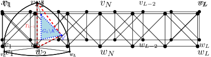
Figure 1: The outer-1-planar graph $G_{8}$, and how to find nested triangles.

It is known that all outer-1-planar graphs have a planar drawing [2], but they can have many different planar embeddings. However, we can show that for our graph $G_{L}$, all planar embeddings are bad in some sense.

Call a set of disjoint triangles $T_{1},\dots,T_{\ell}$ nested (in a fixed planar embedding) if for $i=2,\dots,\ell$ the region bounded by $T_{i}$ includes all vertices of $T_{1}\cup\dots\cup T_{i-1}$.

Lemma 3.1.

Fix $L\geq 2$ even. Any planar embedding $\Gamma$ of $G_{L}$ with $(v_{L},w_{L})$ on the outer-face contains $L/2$ nested triangles.

Proof 3.2.

Set $K:=\{v_{L},w_{L},v_{L-1},w_{L-1}\}$. These four vertices form a $K_{4}$; its induced embedding $\Gamma_{K}$ is hence unique up to renaming. By assumption the outer-face $T$ of $\Gamma_{K}$ contains $v_{L},w_{L}$ and one vertex $y\in\{v_{L-1},w_{L-1}\}$; set $x=\{v_{L-1},w_{L-1}\}\setminus y$.

If $L=2$, then we are done (use triangle $T$). If $L>2$, then graph $G^{\prime}:=G_{L}\setminus K$ is connected, so must reside entirely within one face $f$ of $\Gamma_{K}$. Graph $G^{\prime}$ contains neighbours of $x$ and $y$, so face $f$ must contain both $x$ and $y$. Since $x$ is not on the outer-face of $\Gamma_{K}$, face $f$ is not the outer-face of $\Gamma_{K}$. So no vertex of $G_{L}\setminus K$ is in the outer-face of $\Gamma_{K}$, making $T$ the outer-face of the entire drawing $\Gamma$.

Observe that $G^{\prime}=G_{L}\setminus K$ is a copy of $G_{L-2}$. Since both $v_{L-2}$ and $w_{L-2}$ have neighbours in $\{x,y\}$, edge $(v_{L-2},w_{L-2})$ is on the outer-face of the induced drawing $\Gamma^{\prime}$ of $G^{\prime}$. By induction, $\Gamma^{\prime}$ contains $L/2-1$ nested triangles $T_{1},\dots,T_{L/2-1}$. Adding the outer-face $T$ to this gives the desired set of nested triangles for $G$ since $G_{L-2}$ resides inside $T$ and is vertex-disjoint from it.

Theorem 3.3.

There exists an $n$-vertex outer-1-planar graph that requires width and height at least $n/4$ in any planar poly-line grid-drawing.

Proof 3.4.

Fix an arbitrary integer $N$, and consider graph $G_{4N}$ which has $n=8N$ vertices. Observe that $G_{4N}$ contains two disjoint copies of $G_{2N}$, obtained by removing the edges $(v_{2N},v_{2N+1})$ and $(w_{2N},w_{2N+1})$. In any planar embedding of $G_{4N}$, at least one of these two copies of $G_{2N}$ must have its rightmost/leftmost grid-edge on the outer-face of its induced planar embedding. In this copy, we therefore have $N$ nested triangles by Lemma 3.1. It is known [10] that $\ell$ nested triangles require width and height $2\ell$ in any planar poly-line drawing, which implies the result by $2N=n/4$.

If we use so-called 1-fused stacked triangles [4], then the lower bound can be improved ever-so-slightly to $(n+2)/4$ after inserting a crossing into all inner regions of the $2\times L$-grid; see a preliminary version of this paper [6] for details. We gave the weaker bound here because $G_{L}$ has two other advantages: it is IC-planar (no two crossings have a common vertex) and it has maximum degree 4 (so the lower bound even holds for orthogonal point-drawings).

3.1 Drawing outer-planar graphs, and the approach of [2]

We now briefly review the algorithm by Auer et al. [2] to explain where the error lies. Their algorithm is based on a prior algorithm (we call it here MaxOutpl) by the author that creates an order-preserving orthogonal bar-drawing of any maximal outer-planar graph [3, 4]. The idea MaxOutpl is to fix one reference-edge $(s,t)$ with poles $s,t$ on the outer-face (with $s$ before $t$ in clockwise order). Then draw graph $G$ such that the bars of $s$ and $t$ occupy the top right and bottom right corner respectively.

To do so, split the graph and recurse, see also Figure 2(a). Specifically, consider the interior face incident to $(s,t)$ (say its third vertex is $x$). Of the two subgraphs “hanging” at the edges $(s,x)$ and $(x,t)$, pick the smaller one. (Formally, for any edge $(u,v)\neq(s,t)$, the hanging subgraph $H_{uv}$ is the graph induced by all outer-face vertices between $v$ and $u$, using the path from $v$ to $u$ that does not include edge $(s,t)$.) Assume that $H_{x,t}$ is not bigger than $H_{s,x}$, but has at least three vertices (all other cases are handled symmetrically or with another simpler construction). Let $\{x,y_{1},t\}$ be the other interior face at $(x,t)$. Recursively draw the three subgraphs $H_{s,x}$, $H_{x,y_{1}}$ and $H_{y_{1},t}$ with respect to reference-edges $(s,x),(x,y_{1})$ and $(y_{1},t)$. After a minor modification of the drawings (“releasing” one pole, defined below) and rotating the drawing of $H_{x,y_{1}}$, these drawings can be merged as shown in Figure 2(b).

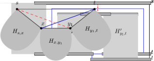
(a)  

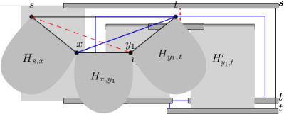
(b)  

(c)  

(d)  

Figure 2: The construction by the author [4] and by Auer et al. [2]. (a) Splitting the graph (the red dashed edge does not exist for outer-planar graphs). (b) Putting drawings together in [4]. (c) Putting drawings together in [2]. (d) A variation of [2].

Auer et al. [2] used the same idea, but release other poles, mirror drawings rather than rotate them, and route edge $(x,t)$ differently. This leaves space free to also route edge $(s,y_{1})$ and removes all bends, hence giving a visibility representation. See Figure 2(c). However, there are a few issues with this construction:

• First, the logarithmic height-bound for MaxOutpl crucially requires that the constructed drawing is no bigger than the drawing of the bigger subgraph $H_{s,x}$. This is violated in the construction from Figure 2(c), though the issue can easily be fixed by drawing one edge horizontally instead, see Figure 2(d).

• Second, Auer et al. silently assume that the region incident to $(s,t)$ has a crossing. If it does not, but if the other region incident to $(x,t)$ has a crossing, then it is not even clear how $y_{1}$ should be picked, and the crossing edges are not both drawn.

• Finally, even if the region at $(s,t)$ has a crossing, the crossing edge need not be $(s,y_{1})$. (Recall that in MaxOutpl vertex $y_{1}$ is determined by the size of the subgraphs and cannot be picked arbitrarily.) Instead, the crossing edge could connect $t$ to a vertex in $H_{s,x}$, and we cannot add such an edge to the drawing without adding bends or going through other bars.

The third issue is the one that led to our counter-example, constructed such that if we pick $\{s,t,x,y_{1}\}$ to be the endpoints of a crossing, then graph $H_{s,x}$ is not the biggest of the subgraph (and neither is $H_{y_{1},t}$), and so the logarithmic height-bound fails to hold.

4 Constructions

It should be quite obvious that if we allow crossings and some bends, then we can create drawings of area $O(n\log n)$ for any outer-1-planar graph $G$. Specifically, pick an arbitrary maximal outer-planar subgraph $G^{-}$ of $G$, and let $\Gamma^{-}$ be an orthogonal bar-drawing of $G^{-}$ obtained with MaxOutpl. Since every edge has at most two bends, every region of $\Gamma^{-}$ has $O(1)$ bends. As such, any edge of $G\setminus G^{-}$ (which needs to be drawn through two adjacent regions) can be inserted with $O(1)$ bends. We now work on reducing this bound on the number of bends and show:

Theorem 4.1.

Any outer-1-planar graph has an order-preserving orthogonal box-drawing with at most two bends per edge and $O(n\log n)$ area.

It is straight-forward to convert any planar orthogonal box-drawing into a poly-line drawing while keeping the area asymptotically the same and adding at most two bends per edge. See [5] for details, and note that the same technique works whether the drawing is planar or not. Therefore our result implies:

Corollary 4.2.

Any outer-1-planar graph has an order-preserving poly-line drawing with at most four bends per edge and $O(n\log n)$ area.

Since we have a constant number of bends per edge, and any outer-1-planar graph has $O(n)$ edges [2], we have $O(n)$ vertical segments in the orthogonal box-drawing. As such, after deleting empty columns if needed, the width is automatically $O(n)$. Therefore all our analysis is focused on the height of the drawing, which we prove to be in $O(\log n)$.

4.1 Drawing types

Now we prove Theorem 3.3 with a recursive drawing algorithm. We roughly follow the idea of MaxOutpl, but explicitly distinguish whether the region incident to $(s,t)$ is crossed or not. Crucially, we allow more types of drawings for the subgraphs to achieve fewer bends overall.

We only draw maximal outer-1-planar graphs; one can always make an outer-1-planar graph maximal by adding edges, and delete those edges from the obtained drawing later. It is known that for a maximal outer-planar graph the edges on the outer-face have no crossing [9].

So fix a maximal outer-1-planar graph $G$ with a fixed outer-1-planar embedding and with reference-edge $(s,t)$. An orthogonal bar-drawing $\Gamma$ of $G$ is called

• a drawing of type A if the bars of $s$ and $t$ occupy the top right and bottom right corner of $\Gamma$, respectively (this is the same as for [4]);

• a drawing of type $\overline{B}$ if the bar of $s$ occupies the top right corner of $\Gamma$, and the bar of $t$ occupies the point one row below this corner;

• a drawing of type $\underline{B}$ if the bar of $t$ occupies the bottom right corner of $\Gamma$, and the bar of $s$ occupies the point one row above this corner;

• a drawing of type C if the bars of $s$ and $t$ occupy the bottom left and bottom right corner of $\Gamma$, respectively.

All drawings that we create are order-preserving. In particular edge $(s,t)$ must be drawn clockwise along the boundary of the drawing; Figure 3 shows how it will be drawn.

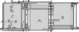
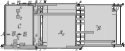
Figure 3: The drawing-types, and the base cases.

Let $\alpha\approx 0.59$ be such that $\alpha^{5}=(1-\alpha)^{3}$. Let $\phi:=\frac{\sqrt{5}-1}{2}\approx 0.618$ be such that $\phi^{2}=1-\phi$. Define $\gamma:=\max\{-\frac{2}{\log\phi},-\frac{3}{\log\alpha}\}\approx\max\{2.88,3.94\}=3.94,$ we hence know

$$\begin{array}[]{ccc}\gamma\log\alpha\leq-3,&&\gamma\log(1{-}\alpha)=\gamma\log(\alpha^{5/3})=\frac{5}{3}\gamma\log\alpha\leq-5\\ \gamma\log\phi\leq-2,&&\gamma\log(1{-}\phi)=\gamma\log(\phi^{2})=2\gamma\log\phi\leq-4,\end{array}$$

Also set $\delta=2$. We measure the size $|G|$ of an $n$-vertex maximal outer-1-planar graph $G$ as $n-1$; this may be rather unusual but will help keep the equations simpler. Define $h(G):=\gamma\log|G|+\delta\approx 3.94\log(n-1)+2$; this is the height that we want to achieve in our drawings. Theorem 4.1 now holds if we show the following result.

Lemma 4.3.

Let $G$ be a maximal outer-1-planar graph with reference-edge $(s,t)$. Then $G$ has order-preserving orthogonal bar-drawings with at most two bends per edge and of the following kind:

• A type-A drawing ${\cal A}$ of height at most $h(G)$,

• a type-$\overline{B}$ drawing $\overline{{\cal B}}$ of height at most $h(G)+2$,

• a type-$\underline{B}$ drawing $\underline{{\cal B}}$ of height at most $h(G)+2$, and

• a type-C drawing ${\cal C}$ of height at most $h(G)+3$.

Furthermore, at least one of $\overline{{\cal B}}$ and $\underline{{\cal B}}$ has height at most $h(G)$.

We prove Lemma 4.3 by induction on $|G|$. In the base case, $G$ consists of only edge $(s,t)$, and one easily constructs suitable drawings, even without bends. See Figure 3. The height is at most 2 in all cases. Since $|G|=1$, we have $\log|G|=0$ and the bound holds by $\delta=2$.

4.2 Subgraphs and tools

Now assume that $n\geq 3$, so $G$ has at least one inner region. The idea is to split $G$ into subgraphs, recursively obtain their drawings, and put them together suitably. We have two cases (see also Figure 4). In Case $\Delta$, the inner region at $(s,t)$ has no crossing; by maximality it is hence a triangle, say $\{s,t,x\}$. We will recurse on the two hanging subgraphs $H_{s,x}$ and $H_{x,t}$, and use $H_{L}:=H_{s,x}$ and $H_{R}:=H_{x,t}$ as convenient shortcuts. Observe that $|H_{L}|+|H_{R}|=|G|$ since we define the size to be one less than the number of vertices. In Case $\times$ the inner region at $(s,t)$ is incident to a crossing, say edge $(s,y)$ crosses edge $(t,x)$. By maximality the edges $(s,x)$, $(x,y)$ and $(y,t)$ exist and have no crossing. We will recurse on the three hanging subgraphs $H_{L}:=H_{s,x}$, $H_{M}:=H_{x,y}$ and $H_{R}:=H_{y,t}$. Observe that $|H_{L}|+|H_{M}|+|H_{R}|=|G|$. These (two or three) subgraphs are smaller, and we assume that they have been drawn inductively, giving drawings ${\cal A}_{L},\overline{{\cal B}}_{L},\underline{{\cal B}}_{L},{\cal C}_{L}$ for subgraph $H_{L}$, and similarly for the other subgraphs. In the pictures, we use ${\cal A}_{L}$ for drawing ${\cal A}_{L}$ rotated by 180 degrees, and similarly for other drawing-types and subgraphs.

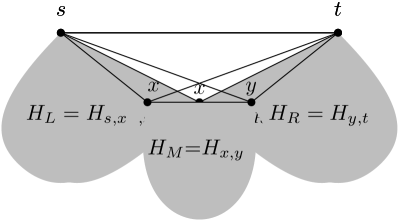
Figure 4: Splitting a subgraph.

To put drawings together, we frequently use two well-known tools [3, 4]:

• If we have a drawing $\Gamma$ of some subgraph, then we can insert empty rows to increase its height since the drawing is orthogonal. If we choose the place to add empty rows suitably, then this does not change the type of the drawing.

• If we have a drawing $\Gamma$ of some subgraph, with vertex $s$ in the top row, then we can release $s$: add a new row above $\Gamma$, let $s$ occupy all of this row, and re-route edges to neighbours of $s$. (If $s$ has a horizontal neighbour $z$, then the edge $(s,z)$ now becomes vertical.) See Figure 5 and [4] for details. This increases the height by 1, and achieves that $s$ now occupies both the top left and top right corner in the resulting drawing $\Gamma^{\prime}$.

  Similarly we can release vertex $t$ to occupy the bottom-left corner, presuming it is drawn in the bottom row. In the pictures, we use a “prime” (e.g. ${\cal A}_{L}^{\prime}$ as opposed to ${\cal A}_{L}$) to indicate that one pole has been released; it will be clear from the picture which one.

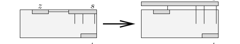
Figure 5: Releasing vertex $s$. Picture taken from [4].

4.3 Induction step—Case $\times$

We start with Case $\times$ where the region incident to $(s,t)$ has a crossing, and study the three different types of drawings that we want to achieve. We occasionally use $h:=h(G)$ as convenient shortcut.

Case $\times$.A: We want a type-A drawing of height $h$. We distinguish sub-cases by the size of $H_{M}$.

Sub-case $\times$.A.1: $|H_{M}|\leq\alpha|G|$ (recall that $\alpha\approx 0.59$). We know that $|H_{L}|+|H_{R}|\leq|G|$, hence we may assume $|H_{R}|\leq|G|/2$ and use construction $\times.A.(a)$ from Figure 6. (The case $|H_{L}|\leq|G|/2$ is symmetric and uses construction $\times.A.(b)$.)

(a)  

(b)  

Figure 6: Constructions for $\times.A$.

We will (for this case only) explain in detail how this figure is to be interpreted; for later cases we hope that the figures alone suffice. We use drawings ${\cal A}_{L},{\cal A}_{M}$ and ${\cal A}_{R}$ of the subgraphs $H_{L},H_{M},H_{R}$. The primes in the figure indicate that we should release release $y$ in both ${\cal A}_{M}$ and ${\cal A}_{R}$ to get ${\cal A}_{M}^{\prime}$ and ${\cal A}_{R}^{\prime}$. Rotate ${\cal A}_{M}^{\prime}$ by $180^{\circ}$ to get ${\cal A}_{M}^{\prime}$ . Increase the height of drawings, if needed, such that ${\cal A}_{R}^{\prime}$ and ${\cal A}_{M}^{\prime}$ have the same height; then combine the two bars of $y$ into one. Increase the height of ${\cal A}_{M}$, if needed, so that it is at least two rows taller than the other two drawings. Then we combine these drawings and route the edges $(s,y),(x,t)$ and $(s,t)$ as shown in Figure 6(a).

One can easily verify that the result is an order-preserving drawing. To argue that it has height at most $h$, the general procedure is as follows. First study the height of all three drawings of subgraphs, which must be at most $h$. Furthermore, at some of these subgraph-drawings more rows are needed, for releasing vertices and/or routing edges and/or other bars. If this is the case, then we must argue that the subgraph-drawing is sufficiently much smaller ($h-3$ in case $\times.A.1$). With this the total height-requirement at most $h$ at this subgraph-drawing, and so other parts of the drawing are not forced to increase beyond height $h$. After arguing this for all three subgraphs, we therefore know that the height of the constructed drawing is at most $h$.

In the specific case here, the height-analysis is done as follows. Since $|H_{L}|\leq|G|$, drawing ${\cal A}_{L}$ has height at most $h(H_{L})\leq h(G)=h$. We have $|H_{M}|\leq\alpha|G|$, so drawing ${\cal A}_{M}$ has height at most

$$h(H_{M}) = \log|H_{M}|+\delta\leq\gamma\log(\alpha\cdot|G|)+\delta=\gamma\log|G|+\delta+\gamma\log\alpha$$

$$= h(G)+\gamma\log\alpha\leq h-3$$

by $\gamma\log\alpha\leq-3$. Since $|H_{R}|\leq\tfrac{1}{2}|G|<\alpha|G|$, likewise ${\cal A}_{R}$ has height at most $h-3$. We need three more rows above ${\cal A}_{M}$ and ${\cal A}_{R}$: one to release $y$, one for edge $(x,t)$ and one for the bar of $s$. So the height requirement is at most $h$ everywhere as desired.

Sub-case $\times$.A.2: $|H_{M}|>\alpha|G|$. We know that one of $\overline{{\cal B}}_{M}$ or $\underline{{\cal B}}_{M}$ has height at most $h(G_{M})$. Let us assume that this is $\underline{{\cal B}}_{M}$, and we then use construction $\times.A.(c)$ from Figure 6 (the other case uses construction $\times.A.(d)$ and is similarly analyzed).

Drawing $\underline{{\cal B}}_{M}$ has height at most $h(G_{M})\leq h$ by assumption. Since $|H_{R}|\leq|G|-|H_{M}|\leq(1-\alpha)|G|$, drawing ${\cal C}_{R}$ has height at most

$$h(H_{R})+3\leq\gamma\log((1-\alpha)|G|)+\delta+3=h(G)+\gamma\log(1-\alpha)+3\leq h-2$$

by $\gamma\log(1-\alpha)\leq-5$. We need two more rows above ${\cal C}_{R}$ (for $(x,t)$ and the bar of $s$) and the height requirement is at most $h$ here. Drawing ${\cal A}_{L}$ has height at most $h(H_{L})$, which by $|H_{L}|\leq(1-\alpha)|G|$ is similarly shown to be at most $h-5$. We need two rows below ${\cal A}_{L}$ (for releasing $x$ and the bar of $y$). Therefore the height requirement is at most $h$ everywhere.

Case $\times$.B: We want two drawings, of type $\overline{B}$, $\underline{B}$. Both have height at most $h+2$, and one has height at most $h$.

Consider first constructions $\times.B.(a)$ for a type-$\overline{B}$ drawing, and $\times.B.(b)$ for a type-$\underline{B}$ drawing, see Figure 7. In both, the drawing of $H_{M}$ has height at most $h(H_{M})+2\leq h+2$. Drawings ${\cal A}_{L}$ and ${\cal A}_{R}$ have height at most $h$, and we need two more rows at them (one to release a pole, one for a bar of a vertex not in the subgraph). So either drawing has height at most $h+2$ as desired.

But we must distinguish cases (and perhaps use a different construction) to achieve that one of the drawings has height at most $h$.

(a)  

(b)  

(c)  

(d)  

Figure 7: Constructions for $\times.\overline{B}$ and $\times.\underline{B}$.

Sub-case $\times$.B.1: $|H_{L}|,|H_{R}|\leq\phi|G|$ (recall that $\phi=(\sqrt{5}-1)/2\approx 0.618$). We know that one of $\overline{{\cal B}}_{M}$ or $\underline{{\cal B}}_{M}$ has height at most $h(G_{M})$. Let us assume that this is $\underline{{\cal B}}_{M}$, and consider again construction $\times.B.(a)$ (in the other case one similarly analyzes construction $\times.B.(b)$).

Drawing $\underline{{\cal B}}_{M}$ by assumption has height at most $h$. Also for $i\in\{L,R\}$ we have $|H_{i}|\leq\phi|G|$ and drawing ${\cal A}_{i}$ has height at most

$$h(H_{i})=\gamma\log|H_{i}|+\delta\leq\gamma\log|G|+\delta+\gamma\log\phi\leq h(G)+\gamma\log\phi\leq h-2$$

since $\gamma\log\phi\leq-2$. We need two further rows at each of ${\cal A}_{L}$ and ${\cal A}_{R}$, so the height requirement is at most $h$ everywhere.

Sub-case $\times$.B.2: $|H_{L}|>\phi|G|$. Use construction $\times.B.(c)$ to obtain a type-$\overline{B}$ drawing, see Figure 7. We know that $|H_{R}|\leq(1-\phi)|G|$ and hence $\underline{{\cal B}}_{R}$ has height at most

$$h(H_{R})+2\leq h(G)+2+\gamma\log(1-\phi)\leq h-2$$

since $\gamma\log(1-\phi)\leq-4$. We need two more rows above it (one to release $t$ and one for the bar of $s$), so the height requirement at ${\cal B}_{R}$ is at most $h$. Similarly the height of ${\cal A}_{M}$ is at most $h(H_{M})\leq h-4$. We need four more rows above it: one row for releasing $y$, one row because ${\cal B}_{R}^{\prime}$ has a row between $y$ and the (released) $t$, one row for $(x,t)$ and one row for the bar of $s$. So the height requirement is at most $h$ everywhere.

Sub-case $\times$.B.3: $|H_{R}|>\phi|G|$. Symmetrically construction $\times.B.(d)$ gives a type-$\underline{B}$ drawing of height $h$.

Case $\times$.C: We want a type-C drawing of height $h+3$.

Sub-case $\times$.C.1: $|H_{M}|\geq\tfrac{1}{2}|G|$. We know that one of $H_{L},H_{R}$ has size at most $\tfrac{1}{2}(|G|-|H_{M}|)\leq\tfrac{1}{4}|G|$. Let us assume that this is $H_{L}$, and we then use construction $\times.C.(a)$ from Figure 8 (the other case uses construction $\times.C.(b)$ and is similarly analyzed).

(a)  

(b)  

(c)  

(d)  

Figure 8: Constructions for $\times.C$.

Drawings ${\cal A}_{M}$ and ${\cal A}_{R}$ both have height at most $h$, and we need three more rows (one to release $y$, one for $(x,t)$ and one for $(s,t)$) so the height requirement here is $h+3$. By $|H_{L}|\leq\tfrac{1}{4}|G|$, drawing ${\cal C}_{L}$ has height at most

$$h(H_{L})+3=\gamma\log|H_{L}|+\delta+3\leq h(G)+\gamma\log(\tfrac{1}{4})+3\leq h-1$$

by $\gamma\geq 2$. We require three more rows above it: one for $(s,y)$, one row that was used for $(x,t)$ elsewhere, and one row for $(s,t)$. So the height requirement here is actually strictly less than $h+3$.

Sub-case $\times$.C.2: $|H_{M}|\leq\tfrac{1}{2}|G|$. We know that one of $H_{L},H_{R}$ has size at most $\tfrac{1}{2}|G|$. Let us assume that this is $H_{R}$, and we then use construction $\times.C.(c)$ from Figure 8 (the other case uses construction $\times.C.(d)$ and is similarly analyzed).

Drawing ${\cal A}_{L}$ has height at most $h$, and we need three more rows (for releasing $x$, edge $(s,y)$ and edge $(s,t)$), so the height requirement here is at most $h+3$. Drawing $\overline{{\cal B}}_{M}$ has height at most

$$h(H_{M})+2\leq h(G)+\gamma\log(\tfrac{1}{2})+2\leq h$$

by $\gamma\geq 2$. Again we need three more rows, so the height requirement is at most $h+3$. Similarly by $|H_{R}|\leq\tfrac{1}{2}|G|$ drawing ${\cal A}_{R}$ has height at most $h-2$. We need five more rows at ${\cal A}_{R}$: one row for releasing $y$, one row because $\overline{{\cal B}}_{M}^{\prime}$ had one row between $y$ and the (released) $x$, one row for $(x,t)$, one row that was used for $(s,y)$ elsewhere, and one row for $(s,t)$. So the height requirement everywhere is at most $h+3$.

4.4 Induction step—Case $\Delta$

Now we turn our attention to the (much simpler) case $\Delta$ where the region incident to edge $(s,t)$ has no crossing. We again distinguish cases by the drawing-type that we want to achieve.

Case $\Delta$.A: We want a type-A drawing of height $h$.

Sub-case $\Delta$.A.1: $|H_{L}|,|H_{R}|\leq\phi|G|$. Then use construction $\Delta.A.(a)$ from Figure 9. Drawing $\overline{{\cal B}_{L}}$ has height at most

$$h(H_{L})+2=\gamma\log|H_{L}|+\delta+2\leq h(G)+\gamma\log\phi+2\leq h$$

since $\gamma\log\phi\leq-2$. Similarly drawing ${{\cal A}_{R}}$ has height at most $h-2$ and we need two more rows above it (for releasing $x$ and the bar of $s$). So the height requirement is at most $h$ everywhere.

(a)  

(b)  

(c)  

Figure 9: Constructions for $\Delta.A$.

Sub-case $\Delta$.A.2: $|H_{L}|>\phi|G|$. Then use construction $\Delta.A.(b)$. Drawing ${\cal A}_{L}$ has height at most $h$. By $|H_{R}|\leq|G|-|H_{L}|\leq(1-\phi)|G|$, drawing ${\cal C}_{R}$ has height at most

$$h(H_{R})+3\leq h(G)+\gamma\log(1-\phi)+3\leq h-1$$

since $\gamma\log(1-\phi)\leq-4$. We require one more row above it (for the bar of $s$), so the height requirement is at most $h$ everywhere.

Sub-case $\Delta$.A.3: $|H_{R}|>\phi|G|$. Symmetrically one proves that construction $\Delta.A.(c)$ has height at most $h$.

Case $\Delta$.B: We want two drawings, of type $\overline{B}$, $\underline{B}$. Both have height at most $h+2$, and one has height at most $h$.

The construction for the type-$\overline{B}$ drawing is in Figure 10(a). Since ${\cal A}_{L}$ and ${\cal A}_{R}$ have height at most $h$, and we need two further rows above ${\cal A}_{R}$, the height requirement is at most $h+2$ everywhere. If $|H_{R}|\leq\tfrac{1}{2}|G|$ then the height of ${\cal A}_{R}$ is at most

$$h(H_{R})\leq h(G)+\gamma\log\tfrac{1}{2}\leq h-2$$

by $\gamma\geq 2$ and so the height requirement is at most $h$ everywhere.

(a)  

(b)  

(c)  

Figure 10: Constructions for $\Delta.\overline{B}$ and $\Delta.\underline{B}$, as well as for $\Delta.C$.

Likewise, the construction of a type-$\underline{B}$ drawing in Figure 10(b) has height at most $h+2$, and if $|H_{L}|\leq\tfrac{1}{2}|G|$ then the height is at most $h$. Since one of $H_{L}$ and $H_{R}$ has size at most $\tfrac{1}{2}|G|$, one of the drawings has height at most $h$.

Case $\Delta.C$: We want a type-C drawing of height at most $h+3$. The construction is shown in Figure 10(c). Since ${\cal A}_{L}$ and ${\cal A}_{R}$ have height at most $h$, and we need two more rows above them (to release $x$ and for edge $(s,t)$), the height is actually at most $h+2$.

4.5 Putting it all together

We have given suitable constructions in all cases, so by induction Lemma 4.3 holds. Using the type-A drawing, we get a drawing of height $3.94\log(n-1)+2$ and width $O(n)$. Therefore Theorem 4.1 holds. Following the proof, one also sees that the drawing can easily be found in linear time, since we can construct the four drawings of each hanging subgraph in constant time from the drawings of its subgraph.

5 Conclusion

In this paper, we pointed out an error in a result by Auer et al., and show that for some outer-1-planar graphs, any poly-line drawing without crossings requires $\Omega(n^{2})$ area. We then studied orthogonal box-drawings of outer-1-planar graphs that achieve small area. We create such drawings (using bars to represent vertices) that have $O(n\log n)$ area and at most 2 bends per edge, and exactly reflect the given outer-1-planar embedding.

We believe that reducing the number of bends per edge should be possible, and in particular, conjecture that we can achieve $O(n\log n)$ area with at most one bend per edge, perhaps at the expense of modifying the 1-planar embedding. On the other hand, finding drawings with 0 bends (i.e., visibility representations) appears difficult. Perhaps bar-1-visibility drawings (where edges are allowed to go through up to one bar of a vertex) may be possible while keeping the area sub-quadratic.

Straight-line drawings of outer-1-planar graphs are also of interest. It is known that there are order-preserving outer-1-planar straight-line drawings of area $O(n^{2})$ [2]. Are there straight-line drawings of sub-quadratic area (again perhaps at the expense of not respecting the 1-planar embedding)?

References

- [1] E. Argyriou, S. Cornelsen, H. Förster, M. Kaufmann, M. Nöllenburg, Y. Okamoto, C. Raftopoulou, and A. Wolff. Orthogonal and smooth orthogonal layouts of 1-planar graphs with low edge complexity. In T. Biedl and A. Kerren, editors, Graph Drawing and Network Visualization (GD 2018), volume 11282 of LNCS, pages 509–523. Springer, 2018.
- [2] C. Auer, C. Bachmaier, F. Brandenburg, A. Gleißner, K. Hanauer, D. Neuwirth, and J. Reislhuber. Outer 1-planar graphs. Algorithmica, 74(4):1293–1320, 2016.
- [3] T. Biedl. Drawing outer-planar graphs in area. In S. Kobourov and M. Goodrich, editors, Graph Drawing (GD’01), volume 2528 of LNCS, pages 54–65. Springer, 2002.
- [4] T. Biedl. Small drawings of outerplanar graphs, series-parallel graphs, and other planar graphs. Discrete and Computational Geometry, 45(1):141–160, 2011.
- [5] T. Biedl. Height-preserving transformations of planar graph drawings. In C. Duncan and A. Symvonis, editors, Graph Drawing (GD’14), volume 8871 of LNCS, pages 380–391. Springer, 2014.
- [6] T. Biedl. Drawing outer-1-planar graphs revisied. In Graph Drawing and Network Visualization (GD’20), LNCS. Springer, 2020. Poster with a short abstract. To appear. See also ArXiV 2009.07106.
- [7] H. Dehkordi and P. Eades. Every outer-1-plane graph has a right angle crossing drawing. Int. J. Comput. Geom. Appl., 22(6):543–558, 2012.
- [8] R. Diestel. Graph Theory, 4th Edition, volume 173 of Graduate texts in mathematics. Springer, 2012.
- [9] R. Eggleton. Rectilinear drawings of graphs. Utilitas Mathematica, 29:149–172, 1986.
- [10] H. de Fraysseix, J. Pach, and R. Pollack. Small sets supporting Fary embeddings of planar graphs. In ACM Symposium on Theory of Computing (STOC ’88), pages 426–433, 1988.
- [11] S. Hong, P. Eades, G. Liotta, and S. Poon. Fáry’s theorem for 1-planar graphs. In J. Gudmundsson, J. Mestre, and T. Viglas, editors, Computing and Combinatorics (COCOON 2012), volume 7434 of LNCS, pages 335–346. Springer, 2012.
- [12] S. Kobourov, G. Liotta, and F. Montecchiani. An annotated bibliography on 1-planarity. Computer Science Review, 25:49–67, 2017.