Second-order Neural Network Training Using Complex-step Directional Derivative

Abstract

While the superior performance of second-order optimization methods such as Newton’s method is well known, they are hardly used in practice for deep learning because neither assembling the Hessian matrix nor calculating its inverse is feasible for large-scale problems. Existing second-order methods resort to various diagonal or low-rank approximations of the Hessian, which often fail to capture necessary curvature information to generate a substantial improvement. On the other hand, when training becomes batch-based (i.e., stochastic), noisy second-order information easily contaminates the training procedure unless expensive safeguard is employed. As a result, first-order methods prevail and remain the dominant solution for modern deep architectures. In this paper, we adopt a numerical algorithm for second-order neural network training. We tackle the practical obstacle of Hessian calculation by using the complex-step finite difference (CSFD) – a numerical procedure adding an imaginary perturbation to the function for derivative computation. CSFD is highly robust, efficient, and accurate (as accurate as the analytic result). This method allows us to literally apply any known second-order optimization methods for deep learning training. Based on it, we design an effective Newton Krylov procedure. The key mechanism is to terminate the stochastic Krylov iteration as soon as a disturbing direction is found so that unnecessary computation can be avoided. During the optimization, we monitor the approximation error in the Taylor expansion to adjust the step size. This strategy combines advantages of line search and trust region methods making our method preserves good local and global convergency at the same time. We have tested our methods in various deep learning tasks. The experiments show that our method outperforms exiting methods, and it often converges one-order faster. We believe our method will inspire a wide-range of new algorithms for deep learning and numerical optimization.

Introduction

Given the training set, we consider a neural network a function $f(w)$ which takes $w\in\mathbb{R}^{N}$, the vector of network parameters as the input and outputs a real loss value. The training starts with an initial guess of $w_{0}$ aiming to improve $w$ over iterations $w_{0},w_{1},\cdots$ until $w_{k}$ is sufficiently close to the minimizer $w^{*}$. At the $k$-th iteration an improvement of $\Delta w_{k}$ is calculated, which updates $w$ by $w_{k+1}=w_{k}+\Delta w_{k}$. One could Taylor expand $f(w_{k+1})$ as:

$$\begin{split}f(w_{k+1})&=f(w_{k}+\Delta w_{k})=f(w_{k})+\nabla f(w_{k})\cdot\Delta w_{k}\\ &+\frac{1}{2}\Delta w_{k}^{\top}\nabla^{2}f(w_{k})\Delta w_{k}+\mathbf{O}(\|\Delta w_{k}\|^{3}).\end{split}$$ (1)

If we ignore the high-order error term of $\mathbf{O}(\|\Delta w_{k}\|^{3}$, $\Delta w_{k}$ can be computed as $\Delta w_{k}=-H_{k}^{-1}g_{k}$, where $g_{k}=\nabla f(w_{k})$ and $H_{k}=\nabla^{2}f(w_{k})$ are the gradient and Hessian of $f(w_{k})$. Eq. (1) lays the foundation of the Newton’s method, which is probably one of the most powerful optimization methods we are aware of, converging at a quadratic rate locally.

Despite the strong desire of harvesting the power of quadratic convergency, Newton’s method is much less used in practice as its advantages are overshadowed by several algorithmic and practical obstacles. First, it is difficult to analytically calculate $H$ for deep networks. Computing $H$ involves a tedious second-order differentiation chain along the net. While some auto differentiation (AD) techniques (Paszke et al. 2017) offer derivative calculations, they often become clumsy for second-order derivatives making the implementation costly, labor-intensive and error-prone. $H$ is a high-dimension dense matrix (i.e., $H\in\mathbb{R}^{N\times N}$). Thus, it should never be explicitly assembled, ruling out all the direct linear solvers like LU or Cholesky. Newton’s method is also numerically sensitive: an ill-conditioned Hessian yields “dangerous” $\Delta w$ and crashes the optimization quickly. Bigger training sets further exacerbate those challenges as we are actually performing online or stochastic optimization by sampling the actual Hessian at each batch, which could be noisy and misleading. Due to these reasons, even we have witnessed several elegant pseudo second-order techniques like SMD (Schraudolph 2002; Martens 2010), AdaGrad (Duchi, Hazan, and Singer 2011), and Shampoo (Gupta, Koren, and Singer 2018; Anil et al. 2020) etc, many of them remain gradient-based or quasi-Newton-like. The information hidden in $H$ is seldom fully exploited.

In this paper, we propose an algorithmic solution that leverages (stochastic) Newton to train deep neural nets using numerically computed Hessian. More precisely, we compute the first- and second-order numerical directional derivative of $\nabla f$ and $f$, which give Hessian-vector products ($Hp$) and Hessian-inner product ($p^{\top}Hp$) for a vector $p$. While this fact has been used previously for machine learning (Schraudolph 2002), we offer a new implementation of this idea with very little extra coding work under commonly-used deep learning frameworks like TensorFlow (Abadi et al. 2016) and PyTorch (Paszke et al. 2019). We name our method complex-step directional derivative or CSDD. Compared with the classic finite difference method (FD) (Forsythe and Wasow 1960), CSDD is highly robust, accurate, and can be easily generalized to higher-order cases. CSDD relieves implementation barriers of second-order training and seamlessly couples with a wide-range of Newton and quasi-Newton based methods (Knoll and Keyes 2004). Based on CSDD, we advocate a novel stochastic Newton Krylov method for second-order network training. Our method integrates advantages of both line search and trust region methods and fully leverages the curvature information whenever it is reliable. Instead of setting a region radius, we watch the Taylor expansion error and early terminate the Krylov iteration as soon as a risky direction is identified. This approach is fundamentally different from other alternatives like least-square CG (LSCG) or Levenberg–Marquardt (LM) method as we do not alter the shape of the optimization manifold. Therefore, every iteration is descent leading to a better loss. We have tested our method in various deep learning scenarios, and our method consistently outperforms existing competitors. We observe strong second-order convergency in many situations, often one-order faster than commonly-used methods like Adam or Shampoo.

Related Work

The prosperity of deep learning architectures and their applications is not possible without the nutrition from underneath optimization and numerical methods. The training procedure in deep learning is normally regarded as a nonlinear optimization, which relies on the information of gradient and/or Hessian of the target function. On the other hand, modern deep networks are often too complex to be analytically formulated, which can only be dealt with differentiable algorithms like backpropagation (Rumelhart, Hinton, and Williams 1986) also known as BP. BP is a special implementation of AD (Al Seyab and Cao 2008; Paszke et al. 2017). It computes the gradient of the loss function via the chain rule, layer by layer along the network. Based on the it, first-order methods such as SGD (Bottou 2010), Adam (Dozat 2016; Kingma and Ba 2014), AdaGrad (Duchi, Hazan, and Singer 2011), RMSprop (Schaul, Zhang, and LeCun 2013; Sutskever et al. 2013), etc. flourish with increased performance and robustness.

The theories of second-order methods have been well studied  (Nocedal and Wright 2006; Ueberhuber 2012). Generalizing BP to retrieve second-order information as in (Becker, Le Cun et al. 1988; Mizutani and Dreyfus 2008) seems quite possible for deep learning at first sight. Yet, its actual deployment is less common than first-order methods. This is probably because AD techniques become cumbersome in higher-order generalization. Overloading the analytic second-order differentiation is significantly more involved than the first-order case (Margossian 2019), and performing first-order differentiation multiple times to obtain a high-order derivative could lead to inefficient and numerically unstable code (Betancourt 2018). For deep learning, Hessian is a dense matrix, and it may not even fit into the memory. Therefore, many research efforts investigate the possibility of simplifying Hessian using for instance, diagonal (Chapelle and Erhan 2011), diagonal block (Botev, Ritter, and Barber 2017; Martens and Grosse 2015; Zhang, Chen, and Liu 2018), and low-rank (Anil et al. 2020; Gupta, Koren, and Singer 2018) approximations. While they are able to circumvent the memory issue, such simplification does not expose the full spectrum of the curvature, and we can barely observe quadratic convergency in practice. We would also like to point out that the phrase “Hessian” in existing literature could be misleading. Some previous contributions regarded the network as a nested function: $f(w)=l\left(P(w)\right)$, where $l(\cdot)$ is the loss function mapping a network prediction $P(w)$ to the final loss value. Instead of computing $H=\nabla^{2}f$, the Jacobian of $P$, $J=\partial P/\partial w$, was used as a Gauss-Newton approximation of $H$ (Martens 2010; Schraudolph 2002; Amari, Park, and Fukumizu 2000). $J^{\top}J$ does partially constitute $H$, and one can quickly verify this fact by examining the second-order chain rule of $f(w)=l\left(P(w)\right)$. Yet, Gauss-Newton method remains a first-other procedure.

On the other hand, Hessian-free (HF) method seems to be a more attractive option. Since $H$ should not be explicitly built, HF only calculates projected $H$ i.e., the Hessian-vector product, which suffices for many non-direct solvers like Newton Krylov methods (Knoll and Keyes 2004). Calculating Hessian-vector product is equivalent to calculating the directional derivative of the gradient. There are several choices out there. We can use symbolic differentiation (SD) method like the $\mathcal{R}\{\cdot\}$ technique (Pearlmutter 1994), a numerical derivative like FD, or AD-based solutions. Unfortunately, none of them offers both efficiency and accuracy. FD is the most efficient, but subject to numerical issues. SD and AD are accurate, which essentially compute the analytic differentiation via the chain rule. However, they suffer a high overhead computation because of axillary data structures used (e.g., the computation graph etc.).

Alternatively, we use CSDD to facilitate HF computation. As to be detailed in the next section, CSDD is robust, accurate, and more efficient than existing AD packages e.g., CSDD is $14\%$ faster than Tensorflow and $27\%$ faster than PyTorch. Based on CSDD, we re-examine the classic Newton-based optimization techniques and bring several non-trivial enhancements/improvements. During the training, we fully leverage the global gradient to sift noisy batches, and investigate computation efforts only to “worthy” batches. We do not try to globally alter pathological curvature as in LSCG or LM. Instead, we identify risky regions and skip unnecessary Hessian-related computation as much as possible. To the best of our knowledge, this method is the first attempt to synergize CSFD with deep learning and offer a full second-order solution. Our experiments demonstrate a strong convergency behavior on various deep learning tasks.

Complex-step Finite Difference

In order to make the paper more self-contained, we start our discussion with a brief review of the finite difference method, its numerical issue of the subtractive cancellation, and its generalization with complex arithmetic.

Subtractive cancellation of finite difference

Given a function $f:\mathbb{R}\rightarrow\mathbb{R}$ differentiable around $x=x_{0}$. Under a small perturbation $h$, $f$ can be first-order Taylor expanded as $f(x_{0}+h)=f(x_{0})+f^{\prime}(x_{0})\cdot h+\mathbf{O}(h^{2})$, leading to the forward finite difference (FFD) scheme:

$$f^{\prime}(x_{0})\approx\frac{f(x_{0}+h)-f(x_{0})}{h}.$$ (2)

Eq. (2) suggests that $h$ should be as small as possible for a good approximation. Unfortunately, as a computer has limited bits to digitalize real numbers, all the floating-point arithmetics have the round-off error (Ueberhuber 2012), a small relative error also known as machine epsilon $\epsilon$. For the double precision of IEEE 754 floating-point standard (IEEE 1985), $\epsilon\approx 1.11\times 10^{-16}$. Normally, the round-off error does not seriously impair the stability or the accuracy of a numerical procedure. However, when $h$ gets smaller, $f(x_{0}+h)$ and $f(x_{0})$ become nearly equal to each other. Subtraction between them would eliminate leading significant digits, and the result after the rounding could largely deviate from the actual value of $f(x_{0}+h)-f(x_{0})$. Some numerical literature e.g., (Nocedal and Wright 2006) considers that central finite difference (CFD) with the form:

$$f^{\prime}(x_{0})\approx\frac{f(x_{0}+h)-f(x_{0}-h)}{2h},$$ (3)

has higher accuracy, with a quadratic error term of $\mathbf{O}(h^{2})$. This conclusion is only licit when the subtractive cancellation does not occur. In reality, CFD could be even more sensitive to a smaller $h$ because of its faster convergent rate.

First-order complex-step finite difference

The subtractive cancellation can be avoided by using the complex-step finite difference (CSFD) (Martins, Sturdza, and Alonso 2003), which is based on the complex Taylor series expansion (Lyness 1968):

$$f^{*}(x_{0}+hi)=f^{*}(x_{0})+f^{*^{\prime}}(x_{0})\cdot{hi}+\mathbf{O}(h^{2}).$$ (4)

Here, we promote a real-value function $f$ to be a complex-value one $f^{*}$ by allowing complex inputs while retaining its original computation procedure. Under this circumstance, we have $f^{*}(x_{0})=f(x_{0})\in\mathbb{R}$ and $f^{*^{\prime}}(x_{0})=f^{\prime}(x_{0})\in\mathbb{R}$. Extracting imaginary parts of both sides in Eq. (4) yields $\mathtt{Im}\big{(}f^{*}(x_{0}+hi)\big{)}=\mathtt{Im}\big{(}f^{*}(x_{0})+f^{*^{\prime}}(x_{0})\cdot{hi}\big{)}+\mathbf{O}(h^{3})$. We then have the first-order CSFD formulation:

$$f^{\prime}(x_{0})=\frac{\mathtt{Im}\big{(}f^{*}(x_{0}+hi)\big{)}}{h}+\mathbf{O}(h^{2})\approx\frac{\mathtt{Im}\big{(}f^{*}(x_{0}+hi)\big{)}}{h}.$$ (5)

It is clear that Eq. (5) does not have a subtractive numerator meaning it only has the round-off error regardless of the size of the perturbation $h$. In addition, the operation of $\mathtt{Im}(\cdot)$ removes the $(hi)^{2}$ term in the complex Taylor expansion reducing the approximation error to $\mathbf{O}(h^{2})$. If $h\sim\sqrt{\epsilon}$ i.e., around $2\times 10^{-24}$ in Fig. 1, CSFD approximation error is at the order of $\epsilon$. Hence, CSFD can be as accurate as analytic derivative as analytic derivative also has round-off of $\epsilon$.

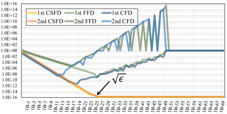
Figure 1: Relative error of different numerical differentiation schemes of $f(x)=e^{x}/(x^{2}+1)$ at $x=10$.

An example is plotted in Fig. 1, where we compare the relative error of numerical derivatives of $f(x)=e^{x}/(x^{2}+1)$ using FFD, CFD, and CSFD with its analytic derivative at $x=10$. The numerical behavior of FFD and CFD is consistent with our analysis: when the perturbation $h$ decreases, CFD converges faster than FFD initially. Both FFD and CFD soon hit the threshold of subtractive cancellation. After that, the relative error bounces back immediately. CSFD reduces the error as quickly as CFD, and the relative error stably remains at the order of $\epsilon$.

Second-order complex-step finite difference

The generalization of CSFD to second- or even higher-order differentiation is straightforward by making the perturbation a multicomplex quantity (Lantoine, Russell, and Dargent 2012; Nasir 2013). The multicomplex number is defined recursively: its base cases are the real set $\mathbb{C}^{0}=\mathbb{R}$, and the regular complex set $\mathbb{C}^{1}=\mathbb{C}$. $\mathbb{C}^{1}$ extends the real set ($\mathbb{C}^{0}$) by adding an imaginary unit $i$ as: $\mathbb{C}^{1}=\{x+yi|x,y\in\mathbb{C}^{0}\}$. The multicomplex number up to an order of $n$ is defined as: $\mathbb{C}^{n}=\{z_{1}+z_{2}i_{n}|z_{1},z_{2}\in\mathbb{C}^{n-1}\}$. Under this generalization, the multicomplex Taylor expansion becomes:

$$\begin{split}&f^{\star}(x_{0}+hi_{1}+\cdots+hi_{n})=f^{\star}(x_{0})+f^{\star^{\prime}}(x_{0})h\sum_{j=1}^{n}i_{j}\\ &+\frac{f^{\star^{\prime\prime}}(x_{0})}{2}h^{2}\big{(}\sum_{j=1}^{n}i_{j}\big{)}^{2}+\cdots+\frac{f^{\star(k)}}{k!}h^{k}\big{(}\sum_{j=1}^{n}i_{j}\big{)}^{k}\cdots.\end{split}$$ (6)

Here, $\left(\sum i_{j}\right)^{k}$ can be computed following the multinomial theorem, and it contains products of mixed $k$ imaginary directions for $k$-th-order terms. The second-order CSFD formulation can then be derived as follows:

$$\begin{array}[]{l}\displaystyle\frac{\partial^{2}f(x,y)}{\partial x^{2}}\approx\frac{\mathtt{Im}^{(2)}\big{(}f(x+hi_{1}+hi_{2},y)\big{)}}{h^{2}},\\ \displaystyle\frac{\partial^{2}f(x,y)}{\partial x\partial y}=\frac{\partial^{2}f(x,y)}{\partial y\partial x}\approx\frac{\mathtt{Im}^{(2)}\big{(}f(x+hi_{1},y+hi_{2})\big{)}}{h^{2}},\end{array}$$ (7)

where $\mathtt{Im}^{(2)}$ picks the mixed imaginary direction of $i_{1}i_{2}$. One can easily tell from Eq. (7) that second-order CSFD is also subtraction-free making them as robust/accurate as the first-order case (e.g., see Fig. 1). Its recursive definition also greatly eases the implementation.

Complex-step Directional Derivative

It may look pointless to have CSDD as the ordinary CSFD alone is able to compute gradient and Hessian accurately. As we will see in this section, CSDD allows us to collectively apply the perturbation along $p$ instead of perturbing every element in $w$. Therefore, CSDD better collaborates with existing deep learning frameworks rather than using CSFD for all the differential operations.

As the name implies, CSDD uses CSFD to calculate projected Hessian under a given direction $p$. For instance, $Hp$ can be written as:

$$[H(w)p]_{a}=\sum_{b=0}^{N-1}\lim_{h\rightarrow 0}\frac{[g(w+he_{b})-g(w)]_{a}}{h}\cdot[p]_{b},$$ (8)

where $[v]_{a}\in\mathbb{R}$ returns $a$-th element in vector $v$; $e_{b}\in\mathbb{R}^{N}$ is a vector with all the elements being zero expect for the $b$-th one, which equals to one. When $h\rightarrow 0$, $[p]_{b}h\rightarrow 0$, and we substitute $h$ with $[p]_{b}h$ to cancel the multiplication of $[p]_{b}$:

$$[H(w)p]_{a}=\sum_{b=0}^{N-1}\lim_{h\rightarrow 0}\frac{[g(w+[p]_{b}he_{b})-g(w)]_{a}}{h}.$$ (9)

Following the linearity of directional derivative, we obtain:

$$Hp=\lim_{h\rightarrow 0}\frac{g(w+hp)-g(w)}{h}\approx\frac{\mathtt{Im}(g(w+hi\cdot p))}{h}.$$ (10)

Similarly, the quadratic form of $p^{\top}Hp$ is the second-order directional derivative $\nabla^{2}_{p}f$. Therefore, we have:

$$\begin{split}p^{\top}Hp&=\lim_{h_{1},h_{2}\rightarrow 0}\frac{h_{1}p^{\top}\big{(}\nabla f(w+h_{2}p)-\nabla f(w)\big{)}}{h_{1}h_{2}}\\ &\approx\frac{\mathtt{Im}^{(2)}(f(w+(hi_{1}+hi_{2})\cdot p))}{h^{2}}.\end{split}$$ (11)

From Eqs. (10) and (11), it is noticed that we only need to apply a single perturbation to compute $Hp$ or $p^{\top}Hp$. This computation can be done with one complex-enabled forward and backward pass of the network. On the other hand, computing $g$ or $H$ requires $N$ and $N^{2}$ perturbations, not to mention the memory consumption. In theory, the CSFD is more efficient than BP or other AD-based subroutines if properly implemented. However, we found CSDD a more feasible option for the purpose of maximizing the re-usability of existing deep learning code. With CSDD, we extract necessary second-order information to devise a full second-order training algorithm, which is to be discussed in the next section.

Stochastic Newton Krylov Optimization

It is known that conjugate gradient (CG) is highly effective for SPD systems with clustered spectra. CG minimizes errors within a Krylov subspace that is iteratively spanned. During the iteration, CG only computes $p^{\top}Hp$ and $Hp$ for a search direction $p$, making itself an ideal HF candidate to solve the Newton step of $H\Delta w=-g$ (Martens 2010; Chapelle and Erhan 2011; Vinyals and Povey 2012; Martens and Sutskever 2011). Here, we discard the subscript $(\cdot)_{k}$ of the Newton iteration index for a more concise notation.

Challenges in stochastic optimization

When $H$ has vanished eigenvalues, CG may experience the division-by-zero issue, and it also diverges if $H$ has negative eigenvalues. In practice, we only know $H$ is symmetric, and there is no guarantee for its positive definiteness. A commonly used strategy is to employ conjugate residual (Saad 2003) or LSCG (Toh and Kojima 2002), which solve a least-square Newton step of $H^{\top}H\Delta w=-H^{\top}g$. The singularity of the system, on the other hand, is overcome by using LM method (Moré 1978) – adding a small diagonal damping to restore the positive definiteness of $H$ or $H^{\top}H$.

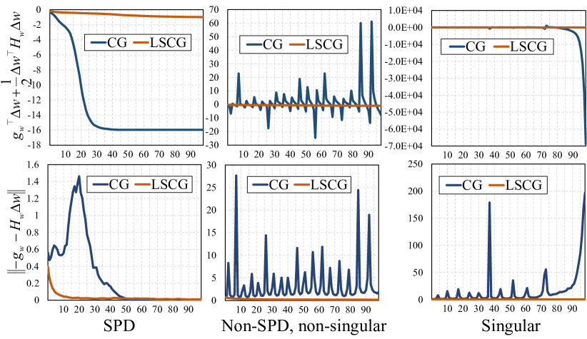
Figure 2: CG is designed to reduce the quadratic energy of $E_{Q}=g^{\top}\Delta w+\frac{1}{2}\Delta w^{\top}H\Delta w$. Focusing on the residual of the linear system could be misleading. LSCG, on the other hand, covers the curvature information and should only be used with extra cautions in stochastic optimization.

Unfortunately, none of these methods offers a true remedy of Newton-CG for deep learning. In stochastic optimization, non positive definiteness suggests either problematic optimization regions or noises in batch-based sampling. We ought to invest computing efforts in neither case. The reason is simple: if the local curvature is misshaped, a complete Newton step that fully solves $H\Delta w=-g$ is unlikely profitable. By projecting this linear system into the column space of $H$, LSCG measures a transformed residual error, which ignores the sign of the curvature; LM evenly “bends” the curvature of the Hessian so that local flatness becomes convex. Clearly, the original curvature information is lost in LSCG and LM. If $w$ is distant from $w^{*}$, such Hessian modifications could adversely affect the global convergency.

Another important observation is that CG is actually an algorithm for minimizing a quadratic energy of:

$$E_{Q}=\Delta w^{\top}g+\frac{1}{2}\Delta w^{\top}H\Delta w,$$ (12)

which is a different measure from the residual error ($\|r\|$). As we can see from the left column of Fig. 2, even with a SPD system, residual error can still go up during CG iterations, while $E_{Q}$ monotonically decreases. When $H$ is singular and semi-SPD, CG iterations also reduce $E_{Q}$ unless a division-by-zero error occurs. However, if $H$ is non-SPD with both positive and negative eigenvalues, CG iterations are in limbo with an oscillating $E_{Q}$ and could diverge any time. Interestingly, it is noted that $E_{Q}$ also appears in the Taylor expansion of $f(w_{k+1})$ i.e., Eq. (1). Since $f(w_{k})$ is a fixed quantity, minimizing $f(w_{k+1})$ is equivalent to minimizing $E_{Q}+\mathbf{O}\|\Delta w\|^{3}$. This implies that if $\mathbf{O}\|\Delta w\|^{3}$ is not the dominating factor in Eq. (1), a CG iteration should be descending under a non-negative curvature.

Our method

Bearing above analysis and observations in mind, we propose an improved stochastic Newton Krylov procedure. Our method is empowered by first- and second-order CSDD (i.e., $\mathtt{CSDD}$ and $\mathtt{CSDD2}$ in Alg. 1). We do not rely on Hessian modifications as in LSCG or LM. Instead, we exploit $\mathtt{CSDD2}$ to switch among different search strategies. Our method significantly improves the convergency performance and is not sensitive to parameter tuning. As one can see from Alg. 1, our algorithm consists of three major subroutines (delimited by dotted lines), which are to be detailed as follows.

1

Input: minibatch set $\{\mathcal{B}_{1},\mathcal{B}_{2},\cdots\}$, $\widetilde{\eta}$

compute $g$; // $g$ is the global gradient

$j\leftarrow 0$; // minibatch index

2 for each $\mathcal{B}_{j}$ do

       compute $g_{j}$; // $g_{j}$ is the local gradient

3       if $g_{j}\cdot g<0$ then

4             $j\leftarrow j+1$;

             continue; // skip this loop for $\mathcal{B}_{j}$

5            

6       end if

      

7       $i\leftarrow 0$, $\quad\Delta w\leftarrow\Delta\widetilde{w}$;

8       $\langle g,h\rangle\leftarrow\mathtt{CSDD}(w,\Delta w)$;

9       $r_{i}\leftarrow-(g+h_{i})$, $\quad p_{i}\leftarrow r_{j}$;

10       while $\|r_{i}\|$ is not small enough do

             $\kappa\leftarrow\mathtt{CSDD2}(w,p_{i})$; // $\kappa=p_{i}^{\top}Hp_{i}$

11             if $\kappa<0$ then

                   break; // early termination

12                  

13             end if

14            if $0<\kappa<1.0\times 10^{-8}$ then

15                   $\kappa\leftarrow 0.01\cdot\|p_{j}\|$;

16             end if

17            $\alpha_{i}\leftarrow\|r_{i}\|/\kappa$;

18             $\Delta w\leftarrow\Delta w+\alpha_{i}p_{i}$;

19             $q_{i}\leftarrow\mathtt{CSDD}(w,p_{i})$;

20             $r_{i+1}\leftarrow r_{i}-\alpha_{i}q_{i}$;

21             $\beta_{j}\leftarrow\|r_{i+1}\|^{2}/\|r_{j}\|^{2}$;

22             $\displaystyle p_{i+1}\leftarrow r_{i+1}+\beta_{i}p_{i}$;

23             $\displaystyle i\leftarrow i+1$;

24       end while

25      if $\Delta w\cdot g>0$ then

26             $\Delta w\leftarrow\big{(}1+\frac{\Delta w\cdot g}{\|\Delta w\|\cdot\|g\|}\big{)}\Delta w$;

27            

28       end if

      

       $\gamma\leftarrow 1$; // the default step size

29       compute $\eta$;

30       if $\eta>0.5\widetilde{\eta}$ then

             $s\leftarrow|\widetilde{\eta}/\eta|$; // an initial test size

31             while $\eta\notin[0.5\widetilde{\eta},\widetilde{\eta}]$ do

32                   if $\eta>\widetilde{\eta}$ then

                         $\gamma\leftarrow 0.5\cdot\gamma$; // shrink a step

33                        

34                   end if

35                  else

                         $\gamma\leftarrow 1.5\cdot\gamma$; // stretch a step

36                        

37                   end if

38                  update $\eta$ with $f(w+\gamma\cdot\Delta w)$;

39             end while

40            

41       end if

42      $w\leftarrow w+\gamma\cdot\Delta w$;

43       compute $g$;

44       $\displaystyle j\leftarrow j+1$;

45 end for

ALGORITHM 1 Our stochastic Newton CG method.

Pre- and post- batch screening

We examine if a minibatch is potentially noisy or unreliable. If yes, we simply skip it to avoid any Hessian computations for this batch. A so-called unreliable batch is defined based on the consistence between local and global gradients: if the batch gradient ($g_{i}$) is opposite to the global gradient ($g$) i.e., $g_{i}\cdot g<0$, the minibatch $\mathcal{B}_{i}$ is discarded.

The post-batch screening occurs after we finish needed Krylov iterations at a local batch. We examine if $\Delta w$ calculated is consistent with negative global gradient $-g$. In theory, Krylov subspace is spanned by conjugating the current residual, and $-g\cdot\Delta w$ is always non-negative. In practice however, as $H$ is sub-sampled, even with pre-batch screening, $\Delta w$ occasionally deviates from $-g$. The post-batch screening removes any search components along $g$ (line 29) so that $\Delta w$ does not cancel previous improvements and remains a global descent.

Krylov loop with early termination

When a minibatch $\mathcal{B}_{i}$ is considered reliable, the algorithm steps into a CG-like Krylov iteration (lines 12 – 27). At each iteration, we monitor the second-order directional derivative of the local loss $\nabla^{2}_{p}f_{i}$ under the search direction $p$. $\nabla^{2}_{p}f_{i}$ reveals the local curvature along $p$, and we terminate the Krylov loop for $\mathcal{B}_{i}$ as soon as $\nabla^{2}_{p}f_{i}$ becomes negative (lines 14 – 16). This negativeness may not reflect the true configuration of the global Hessian but a miss-representation induced by sub-sampling. Therefore, we do not quit the Newton step immediately, but switch to another Hessian sample at the next (reliable) batch. This strategy can also be understood as splitting the full set of global CG iterations over multiple local Hessian samples, and it becomes a classic CG when a local Hessian is highly representative and positive definite. However, it never happens in our experiments, and a local Krylov procedure seldom iterates more than 20 loops.

On the other hand, if $\nabla^{2}_{p}f_{i}$ is close to zero suggesting some local linearity. As discussed before (i.e., see Fig. 2), standard CG still improves $E_{Q}$ in this situation. Therefore, we apply a temporary momentum of $0.01\cdot\|p_{j}\|$ (line 18) to avoid the division-by-zero problem and push the search out of the flat zone. This numerical treatment is different from LM. LM globally and permanently modifies the geometry of the Hessian, while our algorithm alters the curvature locally and temporarily. In addition, LM uses a fixed global damper, which ideally should be just enough to compensate the smallest negative eigenvalue of $H$. Unfortunately, as we are agnostic to $H$ and its spectrum, finding a proper damping is tricky or sometimes even impossible. Our method is adaptive: the local momentum is set based on current search velocity ($0.01\cdot\|p_{i}\|$) – it works robustly by default.

Error-based step sizing

The goal of reducing $f(w_{k+1})$ can be achieved by minimizing $E_{Q}$ only when the quadratic Taylor approximation of $f(w_{k+1})$ is appropriate. In other words, we would like to keep $\mathbf{O}\|\Delta w\|^{3}$ reasonably small during the optimization. This idea has led to several variations of Newton’s method with cubic regularization (Song, Liu, and Jiang 2019; Benson and Shanno 2018), and has been tested in learning tasks (Kovalev, Mishchenko, and Richtárik 2019). We choose a similar but more effective approach with the help of CSDD by directly calculating the Taylor ratio, the ratio between the second-order Taylor approximation error and loss reduction:

$$\eta=|\frac{f(w+\Delta w)-f(w)-E_{Q}}{f(w+\Delta w)-f(w)}|.$$ (13)

Since we only search under positive local curvatures, $\|\Delta w\|$ increases monotonically. Along the iteration of reducing $E_{Q}$, the second-order Taylor approximation also becomes less representative, and $\eta$ accurately measures this trade-off. The global convergency of Newton method is normally implemented by adjusting the step size based on Wolfe conditions (Wolfe 1969, 1971). However, we found that $\eta$ is a more effective tool for this purpose. Specifically, we stretch or shrink the step size $\gamma$ by making sure $\eta$ is within the interval of $[0.5\widetilde{\eta},\widetilde{\eta}]$, where $\widetilde{\eta}$ is the a hyperparameter in our optimization. Because $\Delta w$ is in the same direction of $-g$ (thanks to the post-batch screening), it is guaranteed that a suitable step size always exists. In practice, if the adjustment does not work in few attempts, we simply set the step size small i.e., $\gamma\leftarrow 1.0\times 10^{-6}$. This however, rarely happens.

Restricting $\eta$ being a very small quantity (e.g., $\widetilde{\eta}=0.1\%$) is not encouraged. This is similar to the concept of learning rate in SGD. A very small $\eta$ certainly ensures the convergency but $\Delta w$ does not bring a substantial loss reduction. As a second-order method, $E_{Q}$ is able to approximate $f$ much better than SGD. Therefore, our algorithm is not sensitive to a bigger $\eta$. Unlike learning rate however, $\eta$ is also a relative measure with respect to the actual loss reduction. It is not necessary to frequently adjust this parameter during the optimization.

Discussion

At first sight, our method could appear similar to trust region method (Sorensen 1982), and Taylor ratio $\eta$ resembles the radius of a trust region (normally denoted by $\rho$). A closer look should clarify this confusion: $\rho$ measures the consistence between the reduction of actual loss function and the reduction of $E_{Q}$, while $\eta$ is more straightforward, indicating the percentage of Taylor error in the loss reduction. More importantly, $\eta$ is used in our method to further adjust the step length. This is fundamentally different from trust region methods, which determine $\rho$ beforehand and stop iteration when $\|\Delta w\|>\rho$. We note that doing so makes choosing $\rho$ troublesome. A bigger $\rho$ leads to big Taylor error, and smaller $\rho$ terminates the iteration too early even the local curvature remains sound and positive. On the other hand, our method allows the algorithm to devote necessary efforts to compute a good search direction locally while avoiding computations for problematic curvatures from second-order CSDD. The step size is adjusted by measuring the ratio between the reduction of $f$ and $E_{Q}$. This is a noticeable difference from line search methods, which focus mostly on the loss reduction. Finally, our method does not need pesky parameter tweaking. The only hyperparameter is $\widetilde{\eta}$, which is set as $0.05$ in most experiments.

The convergency analysis of Newton-like method is extensively available in numerical computation textbooks e.g., (Nocedal and Wright 2006; Argyros 2008). The convergency of stochastic Newton method is more involved, yet also well-studied in recent contributions (Kovalev, Mishchenko, and Richtárik 2019; Roosta-Khorasani and Mahoney 2016a, b). Our method is globally convergent and has strong local convergency assuming the Hessian is Lipschitz smooth. We refer the reader to the aforementioned literature for a detailed convergency analysis and move to the experimental study in the next section.

Experiment Results

We implemented our method using CuPy on a desktop PC equipped with an Intel i7-6950X CPU and a nVidia 1080Ti GPU. Some more demanding experiments run on a 2080Ti GPU. Our method has been tested on various deep learning tasks and compared with multiple well-known optimization algorithms including Adam (Kingma and Ba 2014), AdaGrad (Duchi, Hazan, and Singer 2011), Shampoo (Gupta, Koren, and Singer 2018), HF (Martens 2010), and LBFGS (Liu and Nocedal 1989). The results are reported in Fig. 3. In short, our method outperforms all the competing methods in all the experiments by a noticeable margin. A strong quadratic convergency is observed in the tests. We refer the reader to the supplementary document for additional performance analysis. The source code and an illustrative video are also accompanied.

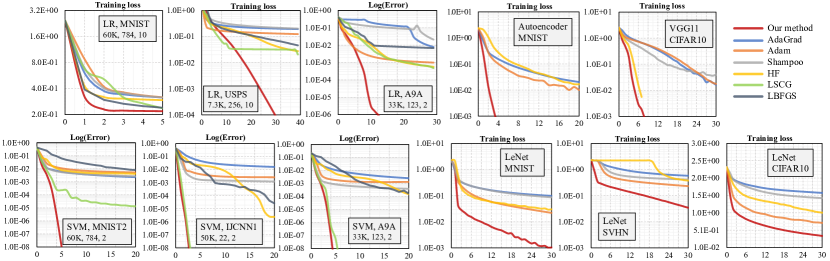
Figure 3: Convergency curves for various deep learning tasks including LR, SVM, autoencoder, and DNNs. The specification of the dataset in LR/SVM tests is also given in the corresponding plot. For instance, 60K, 784, 10 means the total number of training data is 60K. Each date entry has a $784$-dimension feature and will be mapped to $10$ classes/labels.

Performance comparison between CSFD and AD

Before plunging into deep learning tasks, we want to confirm that CSFD is indeed a better approach than AD for derivative calculation. To this end, we record the time of calculating $Hp$ for a VGG-19 net (Simonyan and Zisserman 2014) using autograd from PyTorch (ver. 1.6.0), GradientTape from TensorFlow (ver. 2.3.0), and CSFD. All the experiments run on the single-thread CPU to avoid interference by different parallelization mechanism. We used a naïve CSFD implementation that overloads forward and BP using built-in complex data type from NumPy. CSFD used $58.1~{}sec.$ on average, which is $14\%$ faster than TensorFlow ($66.4~{}sec.$) and $27\%$ faster than PyTorch ($73.4~{}sec.$). It is possible to further accelerate CSFD calculation as in (Luo et al. 2019). Second-order derivative computation with existing AD routines is not yet feasible and potentially unstable.

Regression & SVMs

We compare different training methods for multi-class logistic regression (LR) and support-vector machines (SVMs) using datasets from LIBSVM (Chang and Lin 2011). Each method is trained with a full batch or minibatches of sizes $128$ or $1,024$, and the best result is recorded for the comparison. In SVM training, we used Hinge-2 loss. We note that LSCG is rather close to our method in SVM training. We believe this is because of the good convexity of the Hessian in these experiments. This observation reflects a good adaptivity of our method: if the problem is well-shaped, our algorithm becomes a classic Newton-CG routine. However, LSCG does not yield good results in LR training as the least-square Hessian modification defaces the curvature information, and the Hessian-based computation becomes less effective and downgrades LSCG to be first-order convergent.

Deep Neural Networks

We also evaluate the training convergency on several classic deep neural networks (DNNs) such as deep autoencoder (Kramer 1991), LeNet-5 (LeCun et al. 1998) and VGG-11 (Simonyan and Zisserman 2014). Some methods like vanilla LBFGS and trust region do not work for stochastic training by default. Hence, they are skipped in the corresponding tests. In DNN training, the size of the minibatch is $128$. Our method does not need learning rate tweaking ($\widetilde{\eta}=0.05$). But for other methods, we tried different learning rates from $1.0\times 10^{-1}$ to $1.0\times 10^{-4}$, and the best result is used in the comparison.

Deep autoencoder is trained on MNIST. The architecture of the encoder is $784\rightarrow$ $1,000\rightarrow$ $500\rightarrow$ $250\rightarrow$ $30$. The iterative SVD procedure in Shampoo did not converge, and the corresponding curve is not available. LeNet is a classic DNN architecture with two sets of convolutional layers and average pooling layers, followed by a flattening layer and three FC layers, activated by sigmoid functions. The training is done on MNIST, SVHN, and CIFAR10 datasets. Our experiment also includes the training of a VGG net (VGG-11). The structure of is net is $64\mathtt{Cov}3\rightarrow$ $\mathtt{MP}2\rightarrow$ $128\mathtt{Cov}3\rightarrow$ $\mathtt{MP}2\rightarrow$ $(2\times 256\mathtt{Cov}3)\rightarrow$ $\mathtt{MP}2\rightarrow$ $(2\times 512\mathtt{Cov}3)\rightarrow$ $\mathtt{MP}2\rightarrow$ $(2\times 512\mathtt{Cov}3)\rightarrow$ $\mathtt{MP}2\rightarrow$ $(2\times 512\mathtt{FC})\rightarrow$ $10\mathtt{FC}\rightarrow$ $\mathtt{Softmax}$. We used ELU as the activation function, and the batch normalization is applied before the activation.

Conclusion

In this paper, we propose an effective Newton Krylov algorithm of second-order optimization for deep learning. This algorithm is enabled by a novel implementation of differentiation calculations, namely complex-step finite difference or CSFD. CSFD is essentially a complex-overloaded finite difference procedure, and can be conveniently implemented within existing deep learning frameworks. This convenience leads to a better performance and high-order generalization. In this paper, we use CSFD to compute first- and second-order directional derivatives as an initial proof-of-concept study. Indeed, if properly implemented, CSFD has the potential to largely, if not completely replace existing AD methods. Our contribution goes beyond the introduction of numerical differentiation. With the assistance of CSDD, we bring several important improvements over existing stochastic Newton methods. Guided by both global (e.g., gradient) and local (e.g., curvature) information, our Krylov iteration is keen to noise and concavity, and disturbing computations are largely avoided. We combine the advantages of line search and trust region in the stochastic optimization to ensure each improvement is both effective and substantial.

CSFD and CSDD open a new window for future stochastic optimization. We will investigate its parallel and high-order implementation, and deeply couple carefully-crafted numerical procedures with nonlinear optimizations to empower next-generation deep learning techniques.

References

- Abadi et al. (2016) Abadi, M.; Barham, P.; Chen, J.; Chen, Z.; Davis, A.; Dean, J.; Devin, M.; Ghemawat, S.; Irving, G.; Isard, M.; et al. 2016. Tensorflow: A system for large-scale machine learning. In 12th USENIX Symposium on Operating Systems Design and Implementation (OSDI 16), 265–283.
- Al Seyab and Cao (2008) Al Seyab, R.; and Cao, Y. 2008. Nonlinear system identification for predictive control using continuous time recurrent neural networks and automatic differentiation. Journal of Process Control 18(6): 568–581.
- Amari, Park, and Fukumizu (2000) Amari, S.-I.; Park, H.; and Fukumizu, K. 2000. Adaptive method of realizing natural gradient learning for multilayer perceptrons. Neural computation 12(6): 1399–1409.
- Anil et al. (2020) Anil, R.; Gupta, V.; Koren, T.; Regan, K.; and Singer, Y. 2020. Second Order Optimization Made Practical. arXiv preprint arXiv:2002.09018 .
- Argyros (2008) Argyros, I. K. 2008. Convergence and applications of Newton-type iterations. Springer Science & Business Media.
- Becker, Le Cun et al. (1988) Becker, S.; Le Cun, Y.; et al. 1988. Improving the convergence of back-propagation learning with second order methods. In Proceedings of the 1988 connectionist models summer school, 29–37.
- Benson and Shanno (2018) Benson, H. Y.; and Shanno, D. F. 2018. Cubic regularization in symmetric rank-1 quasi-Newton methods. Mathematical Programming Computation 10(4): 457–486.
- Betancourt (2018) Betancourt, M. 2018. A geometric theory of higher-order automatic differentiation. arXiv preprint arXiv:1812.11592 .
- Botev, Ritter, and Barber (2017) Botev, A.; Ritter, H.; and Barber, D. 2017. Practical gauss-newton optimisation for deep learning. In Proceedings of the 34th International Conference on Machine Learning-Volume 70, 557–565. JMLR. org.
- Bottou (2010) Bottou, L. 2010. Large-scale machine learning with stochastic gradient descent. In Proceedings of COMPSTAT’2010, 177–186. Springer.
- Chang and Lin (2011) Chang, C.-C.; and Lin, C.-J. 2011. LIBSVM: A library for support vector machines. ACM transactions on intelligent systems and technology (TIST) 2(3): 1–27.
- Chapelle and Erhan (2011) Chapelle, O.; and Erhan, D. 2011. Improved preconditioner for hessian free optimization. In NIPS Workshop on Deep Learning and Unsupervised Feature Learning, volume 201. Sierra Nevada Spain.
- Dozat (2016) Dozat, T. 2016. Incorporating nesterov momentum into adam .
- Duchi, Hazan, and Singer (2011) Duchi, J.; Hazan, E.; and Singer, Y. 2011. Adaptive subgradient methods for online learning and stochastic optimization. Journal of machine learning research 12(Jul): 2121–2159.
- Forsythe and Wasow (1960) Forsythe, G. E.; and Wasow, W. R. 1960. Finite Difference Methods. Partial Differential .
- Gupta, Koren, and Singer (2018) Gupta, V.; Koren, T.; and Singer, Y. 2018. Shampoo: Preconditioned stochastic tensor optimization. arXiv preprint arXiv:1802.09568 .
- IEEE (1985) IEEE. 1985. IEEE standard for binary floating-point arithmetic. Institute of Electrical and Electronic Engineers.
- Kingma and Ba (2014) Kingma, D. P.; and Ba, J. 2014. Adam: A method for stochastic optimization. arXiv preprint arXiv:1412.6980 .
- Knoll and Keyes (2004) Knoll, D. A.; and Keyes, D. E. 2004. Jacobian-free Newton–Krylov methods: a survey of approaches and applications. Journal of Computational Physics 193(2): 357–397.
- Kovalev, Mishchenko, and Richtárik (2019) Kovalev, D.; Mishchenko, K.; and Richtárik, P. 2019. Stochastic Newton and Cubic Newton Methods with Simple Local Linear-Quadratic Rates. arXiv preprint arXiv:1912.01597 .
- Kramer (1991) Kramer, M. A. 1991. Nonlinear principal component analysis using autoassociative neural networks. AIChE journal 37(2): 233–243.
- Lantoine, Russell, and Dargent (2012) Lantoine, G.; Russell, R. P.; and Dargent, T. 2012. Using multicomplex variables for automatic computation of high-order derivatives. ACM Transactions on Mathematical Software (TOMS) 38(3): 1–21.
- LeCun et al. (1998) LeCun, Y.; Bottou, L.; Bengio, Y.; and Haffner, P. 1998. Gradient-based learning applied to document recognition. Proceedings of the IEEE 86(11): 2278–2324.
- Liu and Nocedal (1989) Liu, D. C.; and Nocedal, J. 1989. On the limited memory BFGS method for large scale optimization. Mathematical programming 45(1-3): 503–528.
- Luo et al. (2019) Luo, R.; Xu, W.; Shao, T.; Xu, H.; and Yang, Y. 2019. Accelerated complex-step finite difference for expedient deformable simulation. ACM Transactions on Graphics (TOG) 38(6): 1–16.
- Lyness (1968) Lyness, J. 1968. Differentiation formulas for analytic functions. Mathematics of Computation 352–362.
- Margossian (2019) Margossian, C. C. 2019. A review of automatic differentiation and its efficient implementation. Wiley Interdisciplinary Reviews: Data Mining and Knowledge Discovery 9(4): e1305.
- Martens (2010) Martens, J. 2010. Deep learning via hessian-free optimization. In ICML, volume 27, 735–742.
- Martens and Grosse (2015) Martens, J.; and Grosse, R. 2015. Optimizing neural networks with kronecker-factored approximate curvature. In International conference on machine learning, 2408–2417.
- Martens and Sutskever (2011) Martens, J.; and Sutskever, I. 2011. Learning recurrent neural networks with hessian-free optimization. In Proceedings of the 28th international conference on machine learning (ICML-11), 1033–1040. Citeseer.
- Martins, Sturdza, and Alonso (2003) Martins, J. R.; Sturdza, P.; and Alonso, J. J. 2003. The complex-step derivative approximation. ACM Transactions on Mathematical Software (TOMS) 29(3): 245–262.
- Mizutani and Dreyfus (2008) Mizutani, E.; and Dreyfus, S. E. 2008. Second-order stagewise backpropagation for Hessian-matrix analyses and investigation of negative curvature. Neural Networks 21(2-3): 193–203.
- Moré (1978) Moré, J. J. 1978. The Levenberg-Marquardt algorithm: implementation and theory. In Numerical analysis, 105–116. Springer.
- Nasir (2013) Nasir, H. 2013. A new class of multicomplex algebra with applications. Mathematical Sciences International Research Journal 2(2): 163–168.
- Nocedal and Wright (2006) Nocedal, J.; and Wright, S. 2006. Numerical optimization. Springer Science & Business Media.
- Paszke et al. (2017) Paszke, A.; Gross, S.; Chintala, S.; Chanan, G.; Yang, E.; DeVito, Z.; Lin, Z.; Desmaison, A.; Antiga, L.; and Lerer, A. 2017. Automatic differentiation in pytorch .
- Paszke et al. (2019) Paszke, A.; Gross, S.; Massa, F.; Lerer, A.; Bradbury, J.; Chanan, G.; Killeen, T.; Lin, Z.; Gimelshein, N.; Antiga, L.; et al. 2019. PyTorch: An imperative style, high-performance deep learning library. In Advances in Neural Information Processing Systems, 8024–8035.
- Pearlmutter (1994) Pearlmutter, B. A. 1994. Fast exact multiplication by the Hessian. Neural computation 6(1): 147–160.
- Roosta-Khorasani and Mahoney (2016a) Roosta-Khorasani, F.; and Mahoney, M. W. 2016a. Sub-sampled Newton methods I: globally convergent algorithms. arXiv preprint arXiv:1601.04737 .
- Roosta-Khorasani and Mahoney (2016b) Roosta-Khorasani, F.; and Mahoney, M. W. 2016b. Sub-sampled Newton methods II: Local convergence rates. arXiv preprint arXiv:1601.04738 .
- Rumelhart, Hinton, and Williams (1986) Rumelhart, D. E.; Hinton, G. E.; and Williams, R. J. 1986. Learning representations by back-propagating errors. nature 323(6088): 533–536.
- Saad (2003) Saad, Y. 2003. Iterative methods for sparse linear systems, volume 82. siam.
- Schaul, Zhang, and LeCun (2013) Schaul, T.; Zhang, S.; and LeCun, Y. 2013. No more pesky learning rates. In International Conference on Machine Learning, 343–351.
- Schraudolph (2002) Schraudolph, N. N. 2002. Fast curvature matrix-vector products for second-order gradient descent. Neural computation 14(7): 1723–1738.
- Simonyan and Zisserman (2014) Simonyan, K.; and Zisserman, A. 2014. Very deep convolutional networks for large-scale image recognition. arXiv preprint arXiv:1409.1556 .
- Song, Liu, and Jiang (2019) Song, C.; Liu, J.; and Jiang, Y. 2019. Inexact proximal cubic regularized Newton methods for convex optimization. arXiv preprint arXiv:1902.02388 .
- Sorensen (1982) Sorensen, D. C. 1982. Newton’s method with a model trust region modification. SIAM Journal on Numerical Analysis 19(2): 409–426.
- Sutskever et al. (2013) Sutskever, I.; Martens, J.; Dahl, G.; and Hinton, G. 2013. On the importance of initialization and momentum in deep learning. In International conference on machine learning, 1139–1147.
- Toh and Kojima (2002) Toh, K.-C.; and Kojima, M. 2002. Solving some large scale semidefinite programs via the conjugate residual method. SIAM Journal on Optimization 12(3): 669–691.
- Ueberhuber (2012) Ueberhuber, C. W. 2012. Numerical computation 1: methods, software, and analysis. Springer Science & Business Media.
- Vinyals and Povey (2012) Vinyals, O.; and Povey, D. 2012. Krylov subspace descent for deep learning. In Artificial Intelligence and Statistics, 1261–1268.
- Wolfe (1969) Wolfe, P. 1969. Convergence conditions for ascent methods. SIAM review 11(2): 226–235.
- Wolfe (1971) Wolfe, P. 1971. Convergence conditions for ascent methods. II: Some corrections. SIAM review 13(2): 185–188.
- Zhang, Chen, and Liu (2018) Zhang, H.; Chen, W.; and Liu, T.-Y. 2018. On the local Hessian in back-propagation. In Advances in Neural Information Processing Systems, 6520–6530.