Hydrodynamics formalism with Spin dynamics

Abstract

We review the key steps of the relativistic fluid dynamics formalism with spin degrees of freedom initiated recently. We obtain equations of motion of the expansion of the system from the underlying definitions of quantum kinetic theory for the equilibrium phase space distribution functions. We investigate the dynamics of spin polarization of the system in the Bjorken hydrodynamical background.

24.70.+s, 25.75.Ld, 25.75.-q

1 Introduction

Spin polarization experimental measurements of $\Lambda$ hyperons recently taken by the STAR Collaboration [1, 2, 3, 4] have created a huge interest in the spin polarization studies and in studies correlating between the vorticity and particle spin polarization in relativistic heavy-ion collisions[22, 21, 5, 6, 7, 8, 9, 10, 29, 31, 12, 20, 23, 24, 25, 28, 26, 19, 27, 11, 13, 14, 15, 18, 17, 30, 16, 32, 34, 33, 35, 36, 37, 38, 39, 40, 41]; for reviews see[42, 43, 44, 45, 46]. Thermal-based models [47, 48, 49, 50] which precisely explain the global polarization of particles, does able to explain differential results correctly[4], these models assume the condition that particle spin polarization emitted at freeze-out hypersurface is defined by the thermodynamical quantity which is named as thermal vorticity [51, 6], not considering the fact that it may evolve independently during the expansion of the fluid. In this article, we follow scheme proposed in Refs. [52, 53, 54, 55, 56, 57], and analyze such possibility of spin polarization evolution using relativistic hydrodynamics framework with spin.

2 Distribution functions in equilibrium

If we know phase space distribution function for the system’s equilibrium state, then it is possible to derive relativistic hydrodynamics from the underlying kinetic theory definitions[58]. Following ideas developed by Becattini et al.[6], we take into consideration the following distribution functions for the relativistic systems of spin ${\nicefrac{{1}}{{2}}}$ massive particles (and antiparticles) in the local equilibrium state.

$$f^{+}_{rs}(x,p)={\bar{u}}_{r}(p)X^{+}u_{s}(p),\qquad f^{-}_{rs}(x,p)=-{\bar{v}}_{s}(p)X^{-}v_{r}(p),$$ (1)

where $x$ and $p$ is the space-time position coordinate and the four-vector momentum, respectively, with $u_{r}(p)$ and $v_{r}(p)$ being the Dirac bispinors ($r,s=1,2$). Dirac bispinors follow the normalization conditions as ${\bar{u}}_{r}(p)u_{s}(p)=\,\delta_{rs}$ and ${\bar{v}}_{r}(p)v_{s}(p)=-\,\delta_{rs}$, here $\delta_{rs}$ is the Dirac delta function and, $X^{\pm}$ have the following form in terms of relativistic Boltzmann distributions

$$X^{\pm}=\exp\left[\pm\xi(x)-\beta_{\mu}(x)p^{\mu}\pm\frac{1}{2}\omega_{\mu\nu}(x){\Sigma}^{\mu\nu}\right],$$

where $\beta^{\mu}\equiv U^{\mu}/T$ and $\xi\equiv\mu/T$, here $T$, $\mu$ and $U^{\mu}$ is the temperature, baryon chemical potential and four-vector velocity, respectively, and $\omega_{\mu\nu}$ is the second rank asymmetric tensor known as spin polarization tensor with ${\Sigma}^{\mu\nu}\equiv\frac{i}{4}[\gamma^{\mu},\gamma^{\nu}]$ being the spin operator.

With the help of the expressions from Ref. [59] and Eqs. (1) we can obtain the Wigner functions in equilibrium as follows

$${\cal W}^{\pm}_{\rm eq}(x,k) = \frac{e^{\pm\xi}}{4m}\int dP\,e^{-\beta\cdot p}\,\,\delta^{(4)}(k\mp p)$$

$$\times\left[2m(m\pm\not{p})\cosh(\zeta)\pm\frac{\sinh(\zeta)}{2\zeta}\,\omega_{\mu\nu}\,(\not{p}\pm m){\Sigma}^{\mu\nu}(\not{p}\pm m)\right],$$

where $k$ being the off mass-shell particle four-momentum, $dP=d^{3}p/((2\pi)^{3}E_{p})$ is the invariant measure with $E_{p}=\sqrt{m^{2}+{\boldsymbol{p}}^{2}}$ denoting the on-shell energy of the particle, and $\zeta=\frac{1}{2\sqrt{2}}\sqrt{\omega_{\mu\nu}\omega^{\mu\nu}}$ in terms of spin polarization tensor.
Wigner function can also be expanded using Clifford-algebra expansion (2)

$${\cal W}^{\pm}_{\rm eq}(x,k) = \frac{1}{4}\left[{\cal F}^{\pm}_{\rm eq}(x,k)+i\gamma_{5}{\cal P}^{\pm}_{\rm eq}(x,k)+\gamma^{\mu}{\cal V}^{\pm}_{{\rm eq},\mu}(x,k)\right.$$

$$\left.\hskip 28.45274pt+\gamma_{5}\gamma^{\mu}{\cal A}^{\pm}_{{\rm eq},\mu}(x,k)+{\Sigma}^{\mu\nu}{\cal S}^{\pm}_{{\rm eq},\mu\nu}(x,k)\right],$$

where $\mathcal{X}\in\left\{\mathcal{F},\mathcal{P},\mathcal{V}_{\mu},\mathcal{A}_{\mu},\mathcal{S}_{\nu\mu}\right\}$ are the coefficient functions of the Wigner function, which can obtained from the trace of ${\cal W}^{\pm}_{\rm eq}(x,k)$ multiplying first by: $\left\{\mathbf{1},-i\gamma_{5},\gamma_{\mu},\gamma_{\mu}\gamma_{5},2\Sigma_{\mu\nu}\right\}$.

3 Kinetic and hydrodynamical equations

The kinetic equation to be followed by Wigner function is

$$\left(\gamma_{\mu}K^{\mu}-m\right){\cal W}(x,k)=C[{\cal W}(x,k)],$$ (3)

with $K^{\mu}=k^{\mu}+\frac{i\hbar}{2}\,\partial^{\mu}$. For global equilibrium state, the Wigner function follows exactly Eq. (3) with the collision term $C[{\cal W}(x,k)]=0$. The widely used method of treating Eq. (3) is the semi-classical expansion method of the coefficient functions of the Wigner function

$$\mathcal{X}=\mathcal{X}^{(0)}+\hbar\mathcal{X}^{(1)}+\hbar^{2}\mathcal{X}^{(2)}+\cdots.$$

Up to the first order (i.e. next-to-leading order) in $\hbar$ the treatment of Eq. (3) gives the following kinetic equations to be followed by the two independent coefficients which are: $\mathcal{F}_{\mathrm{eq}}$ and $\mathcal{A}_{\mathrm{eq}}^{\nu}$,

$$k^{\mu}\partial_{\mu}\mathcal{F}_{\mathrm{eq}}(x,k)=0,\quad k^{\mu}\partial_{\mu}\mathcal{A}_{\mathrm{eq}}^{\nu}(x,k)=0,\quad k_{\nu}\mathcal{A}_{\mathrm{eq}}^{\nu}(x,k)=0.$$ (4)

In the case of global equilibrium Eqs. (4) are satisfied exactly which in-turn yields the conditions that $\beta_{\mu}$ is a Killing vector, whereas, $\xi$ and $\omega_{\mu\nu}$ are constant, but $\omega_{\mu\nu}$ does not necessarily be equal to thermal vorticity $\varpi_{\mu\nu}=-\frac{1}{2}\left(\partial_{\mu}\beta_{\nu}-\partial_{\nu}\beta_{\mu}\right)=\hbox{const}$. But in the case of local equilibrium Eqs. (4) are not exactly followed, here we follow[60] and by permitting $\beta$, $\xi$ and $\omega$ dependence on $x$, we need to have only certain moments in momentum space of the kinetic equations (4) which are satisfied, which lead to conservation laws for charge, energy-linear momentum and spin[56]

$$\quad\partial_{\mu}N^{\mu}=0,$$ (5)

$$\partial_{\mu}T^{\mu\nu}_{\rm GLW}=0,$$ (6)

$$\partial_{\lambda}S_{\rm GLW}^{\lambda,\alpha\beta}=0,$$ (7)

here the baryon current, the energy-momentum and the spin tensors are based on the forms by the de Groot - van Leeuwen - van Weert (GLW) [59]

$$N^{\alpha} = nU^{\alpha},$$ (8)

$$T^{\alpha\beta}_{\rm GLW} = (\varepsilon+P)U^{\alpha}U^{\beta}-Pg^{\alpha\beta},$$ (9)

$$S^{\alpha,\beta\gamma}_{\rm GLW} = \cosh(\xi)\left[n_{(0)}U^{\alpha}\omega^{\beta\gamma}+{\cal A}_{(0)}\,U^{\alpha}U^{\delta}U^{[\beta}\omega^{\gamma]}_{\hphantom{\alpha}\delta}\right.$$ (11)

$$+\left.\,{\cal B}_{(0)}\,\Big{(}U^{[\beta}\Delta^{\alpha\delta}\omega^{\gamma]}_{\hphantom{\alpha}\delta}+U^{\alpha}\Delta^{\delta[\beta}\omega^{\gamma]}_{\hphantom{\alpha}\delta}+U^{\delta}\Delta^{\alpha[\beta}\omega^{\gamma]}_{\hphantom{\alpha}\delta}\Big{)}\right],$$

where $\Delta^{\alpha\beta}=g^{\alpha\beta}-U^{\alpha}U^{\beta}$ is the spatial projection operator which is orthogonal to the hydrodynamic flow 4-vector $U$.
For the case of polarization tensor in the leading order, the baryon number density, the energy density and, the pressure are expressed respectively as

$$n = \sinh(\xi)\,n_{(0)}(T),$$ (12)

$$\varepsilon = \cosh(\xi)\,\varepsilon_{(0)}(T),$$ (13)

$$P = \cosh(\xi)\,P_{(0)}(T),$$ (14)

where for spin-less and neutral massive Boltzmann particles, thermodynamical properties are defined by[61]

$$n_{(0)}(T) = \frac{2~{}T^{3}}{\pi^{2}}\,\hat{m}^{2}K_{2}\left(\hat{m}\right),$$ (15)

$$\varepsilon_{(0)}(T) = \frac{2~{}T^{4}}{\pi^{2}}\,\hat{m}^{2}\Big{[}3K_{2}\left(\hat{m}\right)+\hat{m}K_{1}\left(\hat{m}\right)\Big{]},$$ (16)

$$P_{(0)}(T) = T\,n_{(0)}(T).$$ (17)

Here, $K_{1}\left(\hat{m}\right)$ and $K_{2}\left(\hat{m}\right)$ are modified Bessel functions of 1st and 2nd kind respectively. The thermodynamical quantities ${\cal B}_{(0)}$ and ${\cal A}_{(0)}$ are expressed as

$${\cal B}_{(0)}=-\frac{2}{\hat{m}^{2}}s_{(0)}(T),\qquad{\cal A}_{(0)}=-3{\cal B}_{(0)}+2n_{(0)}(T)$$ (18)

with entropy density $s_{(0)}=\left(\varepsilon_{(0)}+P_{(0)}\right)/T$ and $\hat{m}=m/T$.

4 Bjorken expansion set-up

Since the spin polarization tensor $\omega_{\mu\nu}$ is a 2nd rank asymmetric tensor, so in analogy to the Faraday electromagnetic field strength tensor, it can be written into electric-like ($\kappa$) and magnetic-like ($\omega$) components

$$\omega_{\mu\nu} = \kappa_{\mu}U_{\nu}-\kappa_{\nu}U_{\mu}+\epsilon_{\mu\nu\alpha\beta}U^{\alpha}\omega^{\beta},$$ (19)

where $\kappa$ and $\omega$ are 4-vectors, orthogonal to fluid flow vector $U_{\mu}$. For longitudinal boost-invariant and transversely homogeneous systems[62, 63], one can write the following basis vectors

$$U^{\alpha} = \frac{1}{\tau}\left(t,0,0,z\right)=\left(\cosh(\eta),0,0,\sinh(\eta)\right),$$

$$X^{\alpha} = \left(0,1,0,0\right),$$

$$Y^{\alpha} = \left(0,0,1,0\right),$$

$$Z^{\alpha} = \frac{1}{\tau}\left(z,0,0,t\right)=\left(\sinh(\eta),0,0,\cosh(\eta)\right),$$ (20)

where longitudinal proper time is defined as $\tau=\sqrt{t^{2}-z^{2}}$ and, the space-time rapidity is defined as $\eta=\half\ln((t+z)/(t-z))$. The normalization conditions satisfied by the basis vectors (20) are

$$U\cdot U=1,$$

$$X\cdot X = Y\cdot Y\,\,=\,\,Z\cdot Z\,\,=\,\,-1,$$

$$X\cdot U\,\, = Y\cdot U\,\,\,\,=\,\,Z\cdot U\,\,=\,\,0,$$ (21)

$$X\cdot Y = Y\cdot Z\,\,=\,\,Z\cdot X\,\,=\,\,0.$$

Using the fact that $\kappa$ and $\omega$ are orthogonal to $U_{\mu}$ and Eqs. (21), $\kappa^{\mu}$ and $\omega^{\mu}$ can be written as

$$\kappa^{\alpha} = C_{\kappa X}(\tau)X^{\alpha}+C_{\kappa Y}(\tau)Y^{\alpha}+C_{\kappa Z}(\tau)Z^{\alpha},$$

$$\omega^{\alpha} = C_{\omega X}(\tau)X^{\alpha}+C_{\omega Y}(\tau)Y^{\alpha}+C_{\omega Z}(\tau)Z^{\alpha},$$ (22)

where one can notice that the scalar functions depend only on proper time $(\tau)$.
Putting Eqs. (22) in Eq. (7) and then using the projection method, we project the resulting tensor on different combination of basis vectors $U_{\alpha}X_{\beta}$, $U_{\alpha}Y_{\beta}$, $U_{\alpha}Z_{\beta}$, $Y_{\alpha}Z_{\beta}$, $X_{\alpha}Z_{\beta}$ and $X_{\alpha}Y_{\beta}$, we get the six equations of motions as

$${\rm diag}\left(\cal{L},\cal{L},\cal{L},\cal{P},\cal{P},\cal{P}\right)\,\,\dot{{\boldsymbol{C}}}={\rm diag}\left({\cal{Q}}_{1},{\cal{Q}}_{1},{\cal{Q}}_{2},{\cal{R}}_{1},{\cal{R}}_{1},{\cal{R}}_{2}\right)\,\,{\boldsymbol{C}},$$ (23)

where ${\boldsymbol{C}}=\left(C_{\kappa X},C_{\kappa Y},C_{\kappa Z},C_{\omega X},C_{\omega Y},C_{\omega Z}\right)$, $\dot{(\dots)}\equiv U\cdot\partial=\partial_{\tau}$ and

$${\cal L}(\tau) = {\cal A}_{1}-\frac{1}{2}{\cal A}_{2}-{\cal A}_{3},$$

$${\cal P}(\tau) = {\cal A}_{1},$$

$${\cal{Q}}_{1}(\tau) = -\left[\dot{{\cal L}}+\frac{1}{\tau}\left({\cal L}+\frac{1}{2}{\cal A}_{3}\right)\right],$$

$${\cal{Q}}_{2}(\tau) = -\left(\dot{{\cal L}}+\frac{{\cal L}}{\tau}\right),$$

$${\cal{R}}_{1}(\tau) = -\left[\dot{\cal P}+\frac{1}{\tau}\left({\cal P}-\frac{1}{2}{\cal A}_{3}\right)\right],$$

$${\cal{R}}_{2}(\tau) = -\left(\dot{{\cal P}}+\frac{{\cal P}}{\tau}\right).$$

with

$${\cal A}_{1} = \cosh(\xi)\left(n_{(0)}-{\cal B}_{(0)}\right),$$

$${\cal A}_{2} = \cosh(\xi)\left({\cal A}_{(0)}-3{\cal B}_{(0)}\right),$$

$${\cal A}_{3} = \cosh(\xi)\,{\cal B}_{(0)},$$

Eqs. (23) implies that the ${C}$ functions evolve independently of each other for the case of Bjorken flow and, ${C}_{\kappa X}$ and ${C}_{\kappa Y}$ (similarly ${C}_{\omega X}$ and ${C}_{\omega Y}$) follows the same form of evolution equations due to the rotational invariance.
Charge current conservation (5) for Bjorken type flow is expressed as

$$\frac{dn}{d\tau}+\frac{n}{\tau}=0$$ (24)

whereas the energy and linear momentum conservation law (6) (after projecting on $U$) yields

$$\frac{d\varepsilon}{d\tau}+\frac{(\varepsilon+P)}{\tau}=0.$$ (25)

5 Particle spin polarization at freeze-out

To calculate the mean spin polarization per particle, the following formula is used [56]

$$\langle\pi_{\mu}\rangle=E_{p}\frac{d\Pi_{\mu}(p)}{d^{3}p}/E_{p}\frac{d{\cal{N}}(p)}{d^{3}p},$$ (26)

with $E_{p}\frac{d\Pi_{\mu}(p)}{d^{3}p}$ being the total value of the Pauli-Lubański vector (after integrating over the freeze-out hypersuface, $\Delta\Sigma_{\lambda}$),

$$E_{p}\frac{d\Pi_{\mu}(p)}{d^{3}p}=-\frac{\cosh(\xi)}{(2\pi)^{3}m}\int\Delta\Sigma_{\lambda}p^{\lambda}\,e^{-\beta\cdot p}\,\tilde{\omega}_{\mu\beta}p^{\beta},$$

and

$$E_{p}\frac{d{\cal{N}}(p)}{d^{3}p} = \frac{4\cosh(\xi)}{(2\pi)^{3}}\int\Delta\Sigma_{\lambda}p^{\lambda}\,e^{-\beta\cdot p},$$

is the total momentum density of both particles and antiparticles with four-momentum given as $p^{\lambda}=\left(m_{T}\cosh y_{p},p_{x},p_{y},m_{T}\sinh y_{p}\right)$.
After performing the the canonical boost [64] of (26), we obtain the polarization vector $\langle\pi^{\star}_{\mu}\rangle$ in the local rest frame of the particle as

$$\langle\pi^{\star}_{\mu}\rangle=-\frac{1}{8m}\left[\begin{array}[]{c}0\\ \\ \left(\frac{p_{x}\sinh y_{p}}{b}\right)a_{i}+\left(\frac{\chi\,p_{x}\cosh y_{p}}{b}\right)a_{j}\!+\!2C_{\kappa Z}p_{y}\!-\!\chi C_{\omega X}{m}_{T}\\ \\ \left(\frac{p_{y}\sinh y_{p}}{b}\right)a_{i}+\left(\frac{\chi\,p_{y}\cosh y_{p}}{b}\right)a_{j}\!-\!2C_{\kappa Z}p_{x}\!-\!\chi C_{\omega Y}{m}_{T}\\ \\ -\left(\frac{m\cosh y_{p}+m_{T}}{b}\right)a_{i}-\left(\frac{\chi\,m\,\sinh y_{p}}{b}\right)a_{j}\\ \end{array}\right],$$

(34)

with $a_{i}=\chi\left(C_{\kappa X}p_{y}-C_{\kappa Y}p_{x}\right)+2C_{\omega Z}m_{T}$, $a_{j}=C_{\omega X}p_{x}+C_{\omega Y}p_{y}$, $b=m_{T}\cosh y_{p}+m$, and $\chi=\left(K_{0}\left(\hat{m}_{T}\right)+K_{2}\left(\hat{m}_{T}\right)\right)/K_{1}\left(\hat{m}_{T}\right)$ and $\hat{m}_{T}=m_{T}/T$.

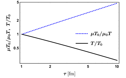
Figure 1: Dependence of the temperature re-scaled by its initial value (solid black line) and the ratio of baryon chemical potential over temperature re-scaled by the initial ratio (dotted blue line) on the proper-time.

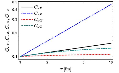
Figure 2: Dependence of scalar functions $C_{\kappa X}$ (solid black line), $C_{\kappa Z}$ (dashed-dotted blue line), $C_{\omega X}$ (dotted red line) and $C_{\omega Z}$ (dashed green line) on the proper-time.

6 Results

Here we show the solutions of the differential equations (23), (24), and (25). System is initialized at the initial proper time $\tau_{0}=1$ fm with initial temperature and the initial baryon chemical potential as $T_{0}=T(\tau_{0})=150$ MeV and $\mu_{0}=\mu(\tau_{0})=800$ MeV, respectively. Here the system is assumed to be formed with $\Lambda$ particles having mass $m=1116$ MeV. In Fig. 1, proper-time dependence of temperature and baryon chemical potential is depicted, where the temperature decreases with proper-time, whereas the ratio of baryon chemical potential and temperature increases with proper-time. From Fig. 2, proper time dependence of the $C$ functions can be known describing the spin polarization evolution of the system.
Using the information of the thermodynamic parameters and $C$ coefficients evolution, we can calculate the different components of the mean polarization vector in the rest frame of the particles $\langle\pi^{\star}_{\mu}\rangle$ at freeze-out, see Fig. 3. We note that $\langle\pi^{\star}_{y}\rangle$ is negative reflecting the system’s initial spin polarization. Because of the Bjorken symmetry which we have assumed in our calculations in this article, the longitudinal component ($\langle\pi^{\star}_{z}\rangle$) of the mean polarization vector is vanishing which is not in agreement with the quadrupole structure of the longitudinal component of the spin polarization seen in the experiment. But we note here that $\langle\pi^{\star}_{x}\rangle$ shows quadrupole structure. We however see and note that the Bjorken set-up is very simple to address the measurements done by the experiment.

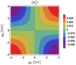
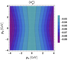
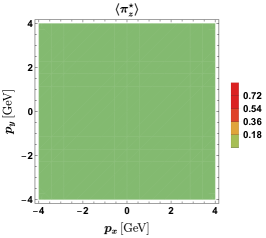
Figure 3: Different components of the mean polarization of $\Lambda$ particles in the rest frame of the particle obtained with the initial values $\mu_{0}=800$ MeV, $T_{0}=155$ MeV, $C_{\kappa,0}=(0,0,0)$ and $C_{\omega,0}=(0,0.1,0)$ for $y_{p}=0$.

7 Summary

We briefly presented the key ingredients of relativistic perfect-fluid hydrodynamics with spin framework initiated recently. From the definitions of kinetic theory for the equilibrium phase space distribution functions in the local equilibrium we obtained the equations of motions for the expansion of the the system. For the case of Bjorken type of flow we investigated the system’s spin polarization dynamics, which in turn show that the scalar functions describing the dynamics of the spin polarization evolve independently of each other. These results are used to obtain the particle spin polarization at the freeze-out hypersurface. We however note that within the current simple set-up of Bjorken symmetry experimental measurements cannot be addressed properly.

References

• [1] L. Adamczyk et al. [STAR Collaboration], Nature 548, 62 (2017).
• [2] J. Adam et al. [STAR Collaboration], Phys. Rev. C 98, 014910 (2018).
• [3] T. Niida [STAR Collaboration], Nucl. Phys. A 982, 511 (2019).
• [4] J. Adam et al. [STAR Collaboration], Phys. Rev. Lett.  123, no. 13, 132301 (2019).
• [5] F. Becattini and L. Tinti, Annals Phys.  325, 1566 (2010).
• [6] F. Becattini et al., Annals Phys.  338, 32 (2013).
• [7] D. Montenegro et al., Phys. Rev. D 96, no. 5, 056012 (2017) Addendum: [Phys. Rev. D 96, no. 7, 079901 (2017)].
• [8] D. Montenegro, L. Tinti and G. Torrieri, Phys. Rev. D 96, no. 7, 076016 (2017)
• [9] F. Becattini, W. Florkowski and E. Speranza, Phys. Lett. B 789, 419 (2019).
• [10] B. Boldizsár, M. I. Nagy and M. Csanád, Universe 5, no. 5, 101 (2019).
• [11] S. Y. F. Liu, Y. Sun and C. M. Ko, Phys. Rev. Lett. 125, no.6, 062301 (2020)
• [12] W. Florkowski et al., Phys. Rev. C 100, no. 5, 054907 (2019).
• [13] H. Z. Wu et al., Phys. Rev. Research.  1, 033058 (2019).
• [14] F. Becattini, G. Cao and E. Speranza, Eur. Phys. J. C 79, no. 9, 741 (2019).
• [15] J. j. Zhang et al., Phys. Rev. C 100, no. 6, 064904 (2019).
• [16] K. Fukushima and S. Pu, arXiv:2001.00359 [hep-ph].
• [17] W. Florkowski, A. Kumar and R. Ryblewski, Acta Phys. Polon. B 51, 945-959 (2020).
• [18] S. Li and H. U. Yee, Phys. Rev. D 100, no. 5, 056022 (2019).
• [19] K. Hattori, Y. Hidaka and D. L. Yang, Phys. Rev. D 100, no. 9, 096011 (2019).
• [20] N. Weickgenannt et al., Phys. Rev. D 100, no. 5, 056018 (2019).
• [21] N. Weickgenannt et al., [arXiv:2005.01506 [hep-ph]].
• [22] S. Shi, C. Gale and S. Jeon, [arXiv:2008.08618 [nucl-th]].
• [23] K. Hattori et al., Phys. Lett. B 795, 100 (2019).
• [24] V. E. Ambrus, JHEP 08, 016 (2020).
• [25] X. L. Sheng, L. Oliva and Q. Wang, Phys. Rev. D 101, no.9, 096005 (2020).
• [26] Y. B. Ivanov, V. D. Toneev and A. A. Soldatov, Phys. Atom. Nucl. 83, no.2, 179-187 (2020).
• [27] Y. Xie, D. Wang and L. P. Csernai, Eur. Phys. J. C 80, no.1, 39 (2020)
• [28] G. Y. Prokhorov, O. V. Teryaev and V. I. Zakharov, Phys. Rev. D 99, no. 7, 071901 (2019).
• [29] G. Y. Prokhorov, O. V. Teryaev and V. I. Zakharov, JHEP 1902, 146 (2019).
• [30] G. Y. Prokhorov, O. V. Teryaev and V. I. Zakharov, JHEP 03, 137 (2020).
• [31] D. L. Yang, Phys. Rev. D 98, no. 7, 076019 (2018).
• [32] Y. Liu and X. Huang, Nucl. Sci. Tech. 31, no.6, 56 (2020).
• [33] S. Tabatabaee and N. Sadooghi, Phys. Rev. D 101, no.7, 076022 (2020).
• [34] S. Bhadury et al., [arXiv:2002.03937 [hep-ph]].
• [35] Y. Liu, K. Mameda and X. Huang, Chin. Phys. C 44, 094101 (2020).
• [36] D. Yang, K. Hattori and Y. Hidaka, JHEP 20, 070 (2020).
• [37] X. Deng et al., Phys. Rev. C 101, no.6, 064908 (2020).
• [38] H. Taya et al. [ExHIC-P], Phys. Rev. C 102, no.2, 021901 (2020).
• [39] J. H. Gao et al., [arXiv:2009.04803 [nucl-th]].
• [40] S. Bhadury et al., [arXiv:2008.10976 [nucl-th]].
• [41] D. Montenegro and G. Torrieri, Phys. Rev. D 102, no.3, 036007 (2020).
• [42] F. Becattini and M. A. Lisa, [arXiv:2003.03640 [nucl-ex]].
• [43] L. Tinti and W. Florkowski, [arXiv:2007.04029 [nucl-th]].
• [44] E. Speranza and N. Weickgenannt, [arXiv:2007.00138 [nucl-th]].
• [45] J. H. Gao et al., Nucl. Sci. Tech. 31, no.9, 90 (2020).
• [46] F. Becattini, [arXiv:2004.04050 [hep-th]].
• [47] F. Becattini et al., Phys. Rev. C 95, no. 5, 054902 (2017).
• [48] I. Karpenko and F. Becattini, Eur. Phys. J. C 77, no. 4, 213 (2017).
• [49] H. Li et al., Phys. Rev. C 96, no. 5, 054908 (2017).
• [50] Y. Xie, D. Wang and L. P. Csernai, Phys. Rev. C 95, no. 3, 031901 (2017).
• [51] F. Becattini, F. Piccinini and J. Rizzo, Phys. Rev. C 77, 024906 (2008).
• [52] W. Florkowski et al., Phys. Rev. C 97, no. 4, 041901 (2018).
• [53] W. Florkowski et al., Phys. Rev. D 97, no. 11, 116017 (2018).
• [54] W. Florkowski, E. Speranza and F. Becattini, Acta Phys. Polon. B 49, 1409 (2018)
• [55] W. Florkowski, R. Ryblewski and A. Kumar, Prog. Part. Nucl. Phys.  108, 103709 (2019).
• [56] W. Florkowski, A. Kumar and R. Ryblewski, Phys. Rev. C 98, no. 4, 044906 (2018).
• [57] W. Florkowski et al., Phys. Rev. C 99, no. 4, 044910 (2019).
• [58] W. Florkowski, M. P. Heller and M. Spalinski, Rept. Prog. Phys.  81, no.4, 046001 (2018)
• [59] S. R. De Groot, W. A. Van Leeuwen, C. G. Van Weert, Relativistic Kinetic Theory, Principles and Applications, Amsterdam, North-Holland, 1980.
• [60] G. Denicol et al., Phys. Rev. D 85, 114047 (2012)
• [61] W. Florkowski, Phenomenology of Ultra-Relativistic Heavy-Ion Collisions, Singapore: World Scientific, 2010.
• [62] J. D. Bjorken, Phys. Rev. D 27, 140 (1983).
• [63] L. Rezzolla and O. Zanotti, Relativistic Hydrodynamics, Oxford University Press, 2013.
• [64] E. Leader, Spin in particle physics, Camb. Monogr. Part. Phys. Nucl. Phys. Cosmol. 15, pp.1-500 (2011)