Efficient Bayesian generalized linear models with time-varying coefficients: The walker package in R

Abstract

The R package walker extends standard Bayesian general linear models to the case where the effects of the explanatory variables can vary in time. This allows, for example, to model the effects of interventions such as changes in tax policy which gradually increases their effect over time. The Markov chain Monte Carlo algorithms powering the Bayesian inference are based on Hamiltonian Monte Carlo provided by Stan software, using a state space representation of the model to marginalise over the regression coefficients for efficient low-dimensional sampling.

Required Metadata

Current code version

Nr.	Code metadata description	Please fill in this column
C1	Current code version	0.4.1
C2	Permanent link to code/repository used for this code version	https://github.com/helske/walker
C3	Code Ocean compute capsule	none
C4	Legal Code License	GPL3
C5	Code versioning system used	git
C6	Software code languages, tools, and services used	R, Stan, C++.
C7	Compilation requirements, operating environments & dependencies	R version 3.4.0 and up, C++14, R packages bayesplot, BH, coda, dplyr, ggplot2, Hmisc, KFAS, methods, rlang, rstan, rstantools, StanHeaders, Rcpp, RcppArmadillo, RcppEigen
C8	If available Link to developer documentation/manual	https://cran.r-project.org/web/packages/walker/walker.pdf
C9	Support email for questions	jouni.helske@iki.fi

Table 1: Code metadata

1 Motivation and significance

Assume a time series of interest $y_{1},\ldots,y_{T}$ which is linearly dependent on the some other predictor time series $X_{1},\ldots,X_{T}$, where $X^{\prime}_{t}=(x_{1t},\ldots,x_{pt})^{\prime}$ are the predictor variables at the time point $t$, and define linear-gaussian time series regression model as

$$y_{t} =X^{\prime}_{t}\beta_{t}+\epsilon_{t},\quad t=1,\ldots,T,$$ (1)

where $\epsilon_{t}\sim N(0,\sigma_{\epsilon}^{2})$ and $\beta$ is a vector of $p$ unknown regression coefficients (first one typically being the intercept term).

It is not always reasonable to assume that the relationship between $y_{t}$ and some predictor $x_{it}$ stays constant over $t=1,\ldots,T$, the time period of interest. The convenient linear relationship approximation may hold well for only piecewise if the underlying relationship is nonlinear or when there are some unmeasured confounders alter the relationship between the measured variables. Allowing the regression coefficients to vary over time can in some instances alleviate these problems. It is also possible that our knowledge of the phenomena of interest already leads to suspect time-varying relationships (see, e.g., Chapter 1 in [1]).

The basic time series regression model (1) can be extended to allow the unknown regression coefficients $\beta_{t}$ to vary over time. This can be done in various ways, for example, by constructing a semiparametric model based on kernel smoothing [2], or parametrically by using dynamic Bayesian networks [3] or state space models [4]. We follow the state space modelling approach and define a gaussian time series regression model with random walk coefficients as

$$y_{t} =X^{\prime}_{t}\beta_{t}+\epsilon_{t},$$ (2)

$$\beta_{t+1} =\beta_{t}+\eta_{t},$$

where $\eta_{t}\sim N(0,D)$, with $D$ being $p\times p$ diagonal matrix with diagonal elements $\sigma^{2}_{i,\eta}$, $i=1,\ldots,p$, and define a prior distribution for the first time point $\beta_{1}$ as $N(\mu_{\beta_{1}},\sigma^{2}_{\beta_{1}})$. The bottom equation in 2 defines a random walk process for the regression coefficients with $D$ defining the degree of variability of the coefficients (with $D=0$ the model collapses to basic regression model).

Our goal is a Bayesian estimation of the unknown regression coefficients $\beta_{1},\ldots,\beta_{T}$ and standard deviations $\sigma=(\sigma_{\epsilon},\sigma_{1,\eta},\ldots,\sigma_{p,\eta})$. Although in principle we can estimate these using the general-purpose Markov chain Monte Carlo (MCMC) software such as Stan [5] or BUGS [6], these standard implementations can be computationally inefficient and prone to severe problems related to the convergence of the underlying MCMC algorithm due to the nature of our models of interest. For example in (block) Gibbs sampling approach we target the joint posterior $p(\beta,\sigma|y)$ by sampling from $p(\beta|\sigma,y)$ and $p(\sigma|\beta,y)$. But because of strong autocorrelations between the coefficients $\beta$ at different time points, as well as with the associated standard deviation parameters, this MCMC scheme can lead to slow mixing. Also, the total number of parameters to sample increases with the number of data points $T$. Although the Hamiltonian Monte Carlo algorithms offered by Stan are typically more efficient exploring high-dimensional posteriors than Gibbs-type algorithms, we still encounter similar problems.

An alternative solution used by the R [7] package walker is based on the property that model (2) can be written as a linear gaussian state space model (see, e.g., Section 3.6.1 in [8]). This allows us to marginalize the regression coefficients $\beta$ during the MCMC sampling by using the Kalman filter leading to a fast and accurate inference of marginal posterior $p(\sigma|y)$. Then, the corresponding joint posterior $p(\sigma,\beta|y)=p(\beta|\sigma,y)p(\sigma|y)$ can be obtained by simulating the regression coefficients given marginal posterior of standard deviations. This sampling can be performed for example by simulation smoothing algorithm [9].

The marginalization of regression coefficients cannot be directly extended to generalized linear models such as Poisson regression, as the marginal log-likelihood is intractable. However, it is possible to use Gaussian approximation of this exponential state space model [10], and the resulting samples from the approximating posterior can then be weighted using the importance sampling type correction [11], leading again to asymptotically exact inference.

When modelling the regression coefficients as a simple random walk, the posterior estimates of these coefficients can have large short-term variation which might not be realistic in practice. One way of imposing more smoothness for the estimates is to switch from random walk coefficients to integrated second order random walk coefficients, defined as

$$\beta_{t+1} =\beta_{t}+\nu_{t},$$

$$\nu_{t+1} =\nu_{t}+\xi_{t},$$

with $\xi_{t}\sim N(0,D_{\xi})$. This is a local linear trend model [12] (also known as an integrated random walk), with the restriction that there is no noise on the $\beta$ level. For this model, we can apply the same estimation techniques as for the random walk coefficient case. More complex patterns for $\beta$ are also possible. For example, we can define that $\beta_{t+1}\sim N(\beta_{t},\gamma_{t}\sigma_{\eta})$ where $\gamma_{1},\ldots,\gamma_{T}$ is known monotonically decreasing sequence of values leading to a case where $\beta_{t}$ gradually converges to constant over time.

2 Software description

A stable version of walker is available at CRAN, while the current development version can be installed from Github. The MCMC sampling is handled by rstan [13], the R interface to Stan, while the model definitions and analysis of the results are performed in R, leading to fast and flexible modelling.

For defining the models, the walker package uses similar Wilkinson-Rogers model formulation syntax [14] as, for example, basic linear model function lm in R, but the formula for walker also recognizes two custom functions, rw1 and rw2 for random walk and integrated random walk respectively. For example, by typing

fit <- walker(y ~ 0 + x +
  rw1(~ z, beta = c(0, 1), sigma = c(0, 1)),
  sigma_y = c(0, 1))

we define a model with time-invariant coefficient for predictor $x$, and first order random walk coefficients for $z$ and time-varying intercept term. Priors for $\beta$ (including the intercept) and $\sigma$ are defined as vectors of length two which define the mean and standard deviation of the normal distribution respectively (for standard deviation parameters the prior is truncated at zero).

Function walker creates the model based on the formula and the prior definitions, and then calls the sampling function from the rstan package. The resulting posterior samples can be then converted to a data frame format using the function as.data.frame for easy visualization and further analysis.

In addition to the main functions walker for the Gaussian case and walker_glm for the Poisson and negative binomial models, the package contains additional functions for visualization of the results (e.g., plot_coef and pp_check) and out-of-sample prediction (function predict). Also, as the modelling functions return the full stanfit used in MCMC sampling, this object can be analysed using many general diagnostic and graphical tools provided by several Stan related R packages such as ShinyStan [15].

3 Illustrative Examples

As an illustrative example, let us consider a observations $y$ of length $n=100$, generated by random walk (i.e. time varying intercept) and two predictors. First we simulate the coefficients, predictors and the observations:

set.seed(1)
n <- 100
beta1 <- cumsum(c(0.5, rnorm(n - 1, 0, sd = 0.05)))
beta2 <- cumsum(c(-1, rnorm(n - 1, 0, sd = 0.15)))
x1 <- rnorm(n, mean = 2)
x2 <- cos(1:n)
rw <- cumsum(rnorm(n, 0, 0.5))
signal <- rw + beta1 * x1 + beta2 * x2
y <- rnorm(n, signal, 0.5)

Then we can call function walker. As noted in Section 2 the model is defined as a simple formula object, and in addition to the prior definitions we can pass various arguments to the sampling method of rstan, such as the number of iterations iter and the number of chains chains to be used for the MCMC (default values for these are 2000 and 4 respectively).

fit <- walker(y ~ 0 + rw1(~ x1 + x2,
  beta = c(0, 10), sigma = c(0, 10)),
  sigma_y = c(0, 10), chains = 2, seed = 1)

The output of walker is walker_fit object, which is essentially a list with stanfit from Stan’s sampling function, the original observations y and the covariate matrix xreg. This allows us to use all the postprocessing functions for stanfit objects.

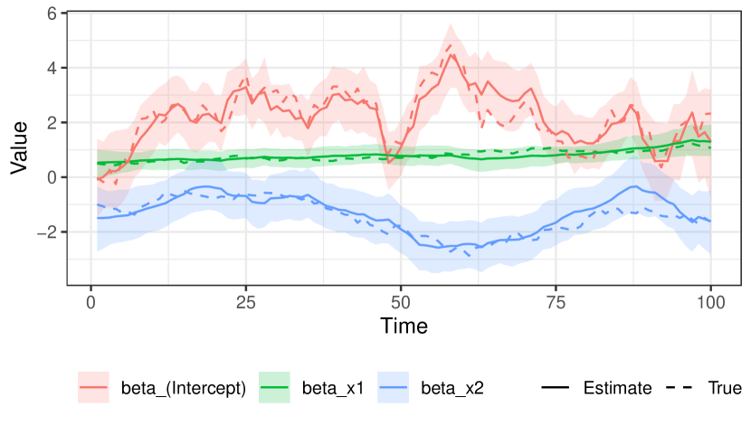
Figure 1 shows how walker recovers the true coefficient processes relatively well: The posterior intervals contain the true coefficients and the posterior mean estimates closely follow the true values. For drawing the figure, we first use function as.data.frame to extract our posterior samples of the coefficients as data frame, then use packages dplyr [16] and ggplot2 [17] to summarise and plot the posterior means and 95% posterior intervals respectively:

library(dplyr)
library(ggplot2)
sumr <- as.data.frame(fit, "tv") %>%
  group_by(variable, time) %>%
  summarise(mean = mean(value), lwr = quantile(value, 0.025),
    upr = quantile(value, 0.975))
sumr$true <- c(rw, beta1, beta2)

ggplot(sumr, aes(y = mean, x = time, colour = variable)) +
  geom_ribbon(aes(ymin = lwr, ymax = upr, fill = variable),
    colour = NA, alpha = 0.2) +
  geom_line(aes(linetype = "Estimate"), lwd = 1) +
  geom_line(aes(y = true, linetype = "True"), lwd = 1) +
  scale_linetype_manual(values = c("solid", "dashed")) +
  theme_bw() + xlab("Time") + ylab("Value") +
  theme(legend.position = "bottom",
    legend.title = element_blank())

Figure 1: Posterior means (solid lines) and 95% posterior intervals (shaded areas) of the time-varying regression coefficients and the true data generating values (dashed lines) of the illustrative example.

More examples can be found in the package vignette and function documentation pages (e.g. typing vignette("walker") or ?walker_glm in R), including a comparison between the marginalization approach of walker and ”naive” implementation with Stan, and an example on the scalability.

4 Impact and conclusions

The walker package extends standard Bayesian generalized linear models to flexible time-varying coefficients case in a computationally efficient manner, which allows researchers in economics, social sciences and other fields to relax the sometimes unreasonable assumption of a stable, time-invariant relationship between the response variable and (some of) the predictors. Similar methods have been previously used in maximum likelihood setting for example in studying the diminishing effects of advertising [18] and demand for international reserves [19].

There are several ways how walker can be extended in the future. There are already some plans for additional forms of time-varying coefficients (such as a stationary autoregressive process), support for more priors and additional distributions for the response variables (e.g., negative binomial).

5 Conflict of Interest

We wish to confirm that there are no known conflicts of interest associated with this publication and there has been no significant financial support for this work that could have influenced its outcome.

References

- [1] M. Moryson, Testing for random walk coefficients in regression and state space models, Springer Science & Business Media, 2012.
- [2] P. M. Robinson, Nonparametric estimation of time-varying parameters, in: Statistical analysis and forecasting of economic structural change, Springer, 1989, pp. 253–264.
- [3] P. Dagum, A. Galper, E. Horvitz, Dynamic network models for forecasting, in: Proceedings of the Eighth Conference on Uncertainty in Artificial Intelligence, UAI ’92, Morgan Kaufmann Publishers Inc., San Francisco, CA, USA, 1992, p. 41–48.
- [4] A. C. Harvey, G. D. A. Phillips, The estimation of regression models with time-varying parameters, in: M. Deistler, E. Fürst, G. Schwödiauer (Eds.), Games, Economic Dynamics, and Time Series Analysis, Physica-Verlag HD, Heidelberg, 1982, pp. 306–321.
-
[5]
Stan Development Team, The Stan C++ Library,
version 2.15.0 (2016).
URL https://mc-stan.org/ - [6] D. J. Lunn, A. Thomas, N. Best, D. Spiegelhalter, WinBUGS - A Bayesian modelling framework: Concepts, structure, and extensibility (Oct 2000). doi:10.1023/A:1008929526011.
[7]
R Core Team, R: A Language and Environment
for Statistical Computing, R Foundation for Statistical Computing, Vienna,
Austria (2020).
URL https://www.R-project.org/ - [8] J. Durbin, S. J. Koopman, Time Series Analysis by State Space Methods, 2nd Edition, Oxford University Press, New York, 2012.
- [9] J. Durbin, S. J. Koopman, A simple and efficient simulation smoother for state space time series analysis, Biometrika 89 (2002) 603–615.
- [10] J. Durbin, S. J. Koopman, Monte Carlo maximum likelihood estimation for non-Gaussian state space models, Biometrika 84 (3) (1997) 669–684.
[11]
M. Vihola, J. Helske, J. Franks,
Importance
sampling type estimators based on approximate marginal MCMC, Scandinavian
Journal of Statistics (2020).
doi:10.1111/sjos.12492.
URL https://onlinelibrary.wiley.com/doi/abs/10.1111/sjos.12492 - [12] A. C. Harvey, Forecasting, Structural Time Series Models and the Kalman Filter, Cambridge University Press, 1990.
[13]
Stan Development Team, RStan: the R interface
to Stan, R package version 2.14.1 (2016).
URL https://mc-stan.org/ -
[14]
G. N. Wilkinson, C. E. Rogers,
Symbolic description of factorial
models for analysis of variance, Journal of the Royal Statistical Society.
Series C (Applied Statistics) 22 (3) (1973) 392–399.
URL https://www.jstor.org/stable/2346786 -
[15]
Stan Development Team, shinystan: Interactive
Visual and Numerical Diagnostics and Posterior Analysis for Bayesian Models,
R package version 2.3.0 (2017).
[16]
H. Wickham, R. François, L. Henry, K. Müller,
dplyr: A Grammar of Data
Manipulation, R package version 0.7.6 (2018).
URL https://CRAN.R-project.org/package=dplyr -
[17]
H. Wickham, ggplot2: Elegant Graphics for
Data Analysis, Springer-Verlag New York, 2016.
URL https://ggplot2.tidyverse.org - [18] H. W. Kinnucan, M. Venkateswaran, Generic advertising; and the structural heterogeneity hypothesis, Canadian Journal of Agricultural Economics/Revue canadienne d’agroeconomie 42 (3) (1994) 381–396. doi:10.1111/j.1744-7976.1994.tb00032.x.
[19]
M. Bahmani-Oskooee, F. Brown,
Kalman filter approach to
estimate the demand for international reserves, Applied Economics 36 (15)
(2004) 1655–1668.
doi:10.1080/0003684042000218543.
URL https://doi.org/10.1080/0003684042000218543