[table]capposition=top \newfloatcommandcapbtabboxtable[][\FBwidth]
RaLL: End-to-end Radar Localization on Lidar Map Using Differentiable Measurement Model
Abstract
Compared to the onboard camera and laser scanner, radar sensor provides lighting and weather invariant sensing, which is naturally suitable for long-term localization under adverse conditions. However, radar data is sparse and noisy, resulting in challenges for radar mapping. On the other hand, the most popular available map currently is built by lidar. In this paper, we propose an end-to-end deep learning framework for Radar Localization on Lidar Map (RaLL) to bridge the gap, which not only achieves the robust radar localization but also exploits the mature lidar mapping technique, thus reducing the cost of radar mapping. We first embed both sensor modals into a common feature space by a neural network. Then multiple offsets are added to the map modal for exhaustive similarity evaluation against the current radar modal, yielding the regression of the current pose. Finally, we apply this differentiable measurement model to a Kalman Filter (KF) to learn the whole sequential localization process in an end-to-end manner. The whole learning system is differentiable with the network based measurement model at the front-end and KF at the back-end. To validate the feasibility and effectiveness, we employ multi-session multi-scene datasets collected from the real world, and the results demonstrate that our proposed system achieves superior performance over driving, even in generalization scenarios where the model training is in UK, while testing in South Korea. We also release the source code publicly 111The code of RaLL is available at https://github.com/ZJUYH/RaLL and a video demonstration is available at https://youtu.be/a3wEv-eVlcg..
Index Terms:
Radar localization, deep learning, differentiable model, kalman filterI Introduction
Localization is a fundamental component for autonomous vehicles. A basic technique is to localize the vehicle via Global Positioning/Inertial Navigation System (GPS/INS) in outdoor scenes, which is infeasible in GPS-denied environments. Localization can also be accumulated by odometry data, while it is impracticable when the drift error becomes significant. Therefore, localization on pre-built map is indispensable, which tracks the robot pose with bounded uncertainty.
Recently many visual and lidar based approaches have been widely proposed in the field of robotics, but there still exist some difficulties in real applications. For instance, visual localization on visual map [1] and lidar map [2] are still challenging when appearance changes significantly, like weather or season varies. For lidar localization, the technique is more mature, pose estimation can be achieved across day and night via point cloud registration [3, 4]. Therefore, city scale lidar maps have been built for preparing commercial applications [5, 6]. Unfortunately, in extreme weather conditions [7], like foggy and snowy, the lidar range measurements are very noisy, calling for the aid of other sensors.
To build a robust localization system, we consider radar is a good choice, which is naturally lighting and weather invariant. Therefore, radar odometry becomes a research focus recently [8, 9, 10, 11, 12], and radar Simultaneous Localization and Mapping (SLAM) [13]. A general idea is to build a map using radar, then localize the vehicle by aligning the radar measurements against the radar map. However, the raw radar data is noisy and sparse actually, and radar data processing is challenging for precise mapping, thus making radar mapping and localization unapplicable. In addition, considering that the large-scale lidar map is available, we argue that repeating the whole mapping process for radar is extremely time and manual labor consuming, also bringing extra calibration between radar map and lidar map [14].
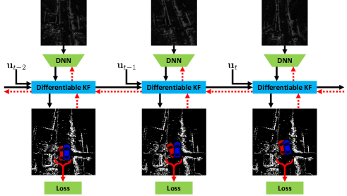
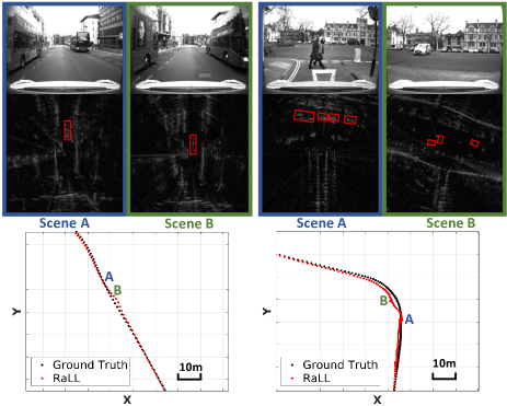
In this paper, we propose an end-to-end learning system to achieve radar based localization directly on lidar maps, as shown in Figure 1. There are two challenges for RaLL. First, the common feature space of the two sensor modals is not explicitly supervised. We propose a network to learn the feature shared embeddings from the pose supervision by introducing a differentiable pose estimator to back-propagate the gradient. Second, after measuring the pose offset of radar and lidar, the uncertainty modeling of this measurement is not explicitly supervised by the network, preventing the probabilistic fusion between measurement and motion model. To address this problem, we apply the learned measurement model in a pose tracking Kalman Filter, enforcing the measurement uncertainty to be compatible to Gaussian fusion. By modeling the whole localization process as a sequential Gaussian distribution estimator, we can supervise the measurement uncertainty via maximizing likelihood. To evaluate the system performance, we utilize RobotCar dataset [15, 16] for benchmark. In addition, the MulRan dataset [17] is employed for testing the generalization of RaLL. In summary, the contributions of this paper are as follows:
-
•
A deep neural network architecture is proposed to learn the cross-modal shared feature embedding by back-propagating gradient from the pose supervision, which leverages the lidar map for radar localization.
-
•
With the learned network being a differentiable measurement model, a Kalman Filter is proposed to generate fused estimation, which is learned in an end-to-end way to improve the accuracy.
-
•
We conduct the model training and testing using RobotCar driving dataset (UK), and achieve similar experimental performance in Mulran dataset (South Korea), demonstrating good generalization of RaLL.
The rest of this paper is organized as follows: Section II reviews the related topics in recent years. The whole system is introduced in Section III. Section IV reports the experimental results on two datasets. We conclude a brief overview of our system and a future outlook in Section V.
II Related Work
II-A SLAM and Localization on Pre-built Maps
SLAM is widely used to construct maps in an unknown environment while simultaneously keeping track of the robot pose. Some visual SLAM [18, 19] and lidar SLAM [20] were proposed to track the vehicle pose in the outdoor scenes. However, there remain some challenging problems in SLAM problem [21], for example, the SLAM performance degradation with dynamics [22, 23] and the adverse weathers [13].
Compared to the SLAM systems, localization on pre-built maps is a more desired technique, especially for long-term autonomy. The localization on pre-built maps avoids the online mapping session, thus making the localization more efficient. Some researchers proposed visual localization on visual maps [24] and lidar maps [2], and also the lidar localization on lidar maps [25]. However, visual or lidar localization is still challenging in adverse weathers. Compared to these two sensors, radar sensor provides lighting and weather invariant sensing. So in this paper, we propose a radar localization on pre-built lidar maps, in which high definition lidar maps are constructed offline and then radar localization is performed.
II-B Localization Using Radar Sensor
Radar sensor has been applied for various perception tasks widely in autonomous driving area, mainly focused on dynamic objects detection on roads. Some researchers achieved indoor positioning using low-cost radar sensors, including localization on Computer Aided Design (CAD) model [26] or laser map [27]. But in challenging outdoor scenarios, precise radar localization is blocked by diverse types of sensor noises and Doppler velocity, therefore, most of studies are based on data pre-processing and sensor modeling [28, 29, 30, 31], or combined with other sensors on vehicles [32].
Recently the Navtech Frequency Modulated Continuous Wave (FMCW) radar sensor brings less Doppler effect, higher resolution and 360∘-view in data collection [15, 16, 17, 13, 33]. The development of this sensor technique results in new approaches to robotic localization research. For place recognition, part of positioning system, researchers extended the existing methods in vision or lidar community to radar data [34, 35, 17]. As for ego-motion estimation, sparse landmarks and keypoints are extracted manually to build efficient data association model [8, 9], and these salient keypoints or pixels can also be learned by neural networks in [10, 36]. The state-of-the-art odometric performance was presented in [11], in which an end-to-end radar odometry system was proposed with the supervision of ground truth poses.
Considering the unavoidable drift in odometry, the registration between live scan and prior map is still essential for long-term localization. Hong et al. [13] used conventional SLAM algorithms to build a radar mapping system. Localization with multiple sensor modalities was presented in [37], in which radar data is localized against satellite images with a coarse initial estimate. The authors then presented more accurate results using multiple networks in [38]. In [39], to connect radar scan and lidar map, a Generative Adversarial Network (GAN) was used to transfer the radar to fake lidar data, and then Monte Carlo Localization (MCL) was applied for pose tracking.
II-C Deep Learning based Localization
With the advances of machine learning, some geometric or theoretical problems of robot localization and mapping were solved by data-driven [40, 41, 42]. A direct way is to localize the sensor by end-to-end learning without geometric information [43], which requires large training data to avoid overfitting. Some researchers [44] established feature correspondences by deep learning and used traditional solvers for pose estimation, while these solvers are indifferentiable for end-to-end learning.
This paper is inspired by several recent deep learning based approaches [6, 11, 5]. In these research works, localization is performed on same sensor modalities. While in this paper, we model the similarity measure and pose regression on the different modalities via deep neural networks. We also train and test the networks with the sequential data, thus building an end-to-end localization system in time domain.
III Methods
The framework of RaLL is a differentiable Kalman Filter embedded with a neural network based measurement model, which is introduced in Section III-C. The network architecture of the measurement model consists of two stages. The first stage embeds the radar scan and lidar map into a common feature space, which is introduced in Section III-A. The second stage evaluates the similarity of the features extracted from two branches above, and yields the final estimation, which is introduced in Section III-B. Finally, we show the training strategy for RaLL in Section III-D.
III-A Comparable Feature Embeddings
We represent both radar scan and lidar map as bird-eye view images. At time , one scan is generated from the radar, and an initial estimation of the pose is . For the prior 2D laser map , we crop it to at pose . With the input and , a neural network is designed to estimate the offset between and the ground truth pose . Therefore, the ground truth offset is the supervision for training .
There are three differences between the data from radar and lidar map, which prevents the direct alignment. First, various types of noises exist in radar data, while the lidar map is much cleaner. Second, there are occlusions in the current scan, while the lidar map is more completed because of the multi-frame integration. Finally, the raw data forms are different: has continuous radar intensities while are represented by binary, or lidar grids. We embed the two heterogeneous modalities into a comparable feature space by training a deep neural network.
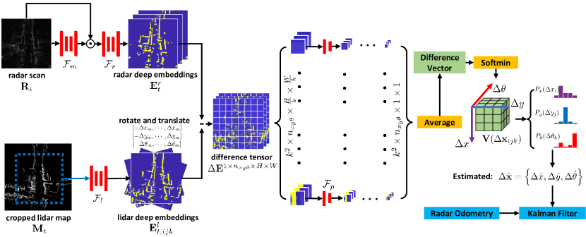
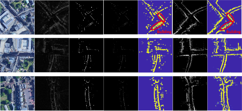
We establish a two-stream neural network for radar and lidar, shown in Figure 2. The whole network consists of three U-Net architectures [45], denoted as , and . To suppress the noise in radar, we apply a masking network to learn a noise mask as in [11]. The sigmoid activation in the final layer constrains the masking output range to , then a de-noised representation is obtained by element-wise multiplication . We notice that the filtered is much clearer as shown in Figure 3. Then we learn the feature embedding which is comparable between the de-noised radar scan and the lidar map: , . We set the final activation function as ReLU in and for feature extraction. Figure 3 demonstrates several learned deep embeddings. It is clear that the features salient in both modalities, are directly comparable in the feature embedding space, such as buildings facade etc.
III-B Similarity-based Offset Estimation
Given the initial pose , the pose offset should lie in a limited interval, denoted as ; the same for and in the range and . Then we divide the 3D solution space for the offset into grids with certain resolutions , and there are candidates in total, e.g. . Hence each candidate in the solution space is denoted as , where . As a result, the absolute pose of each candidate is calculated by transforming the initial pose using the offset as follow:
| (1) |
where , and stand for transformation process, the current pose and pose offset respectively.
At the level of feature embeddings, if the vehicle rotates and translates with the offset , the surrounding map will change respectively. In this context, we rotate and translate the map embedding using candidates, resulting in map blocks . Specifically, for every element in , the transformed element in is calculated with the offset as follows:
| (2) |
where , and are variables in offset .
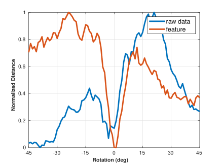
As shown in Figure 3, after the feature embeddings and are learned, we suppose the features should be more comparable than the raw data by the element-wise subtraction . To validate this hypothesis, we rotate the raw map and embeddings of the first scene in Figure 3, and then measure the distance compared to the radar data and embedding respectively. The normalized distance in Figure 4 shows that the substraction of feature embeddings achieves the minimum cost at the ground truth pose, indicating that the learned features are more comparable. Repeating the subtraction for each candidate, we form a difference tensor as with the size , which is the start point for the following similarity learning.
Considering the occlusion, we further divide into small patches as shown in Figure 2. For each patch, we utilize a patch network to derive a patch based difference. Finally, we average the patch based differences and obtain a difference score between the radar scan feature and each candidate , leading to a difference vector with a length of .
Essentially, if a candidate pose, say is close to the ground truth pose , should be similar with , hence leading to a low difference at the th position of the difference vector. As the lower the difference is, the closer the candidate and the ground truth lie, we take a softmin module to transform and normalize the difference vector to form a probability distribution. Then, we reshape the distribution into a 3-dimensional cost volume . In summary, from the current radar scan and the lidar map, the proposed network produces a probability distribution of the pose offset to be estimated, which states as follows:
| (3) |
where is the neural network and is the cost volume.
We then sum over the values along each axis to derive the marginal distribution:
| (4) |
in which the probabilities , and are obtained along the axes in the cost volume .
Upon the marginal distribution, we design two losses to train the network: . When the estimation problem is regarded as three separated classification problems of , a cross entropy loss can be formed as follows:
| (5) |
where , and are one hot encodings of the ground truth, which is the supervision. On the other hand, as a regression problem, we utilize the marginal expectations of the three marginal distributions as the estimators:
| (6) |
where the estimated pose offset is obtained. Then the second loss is constructed by the squared error between and ground truth as follows:
| (7) |
where is a constant value to balance the translation metric and rotation angle metric .
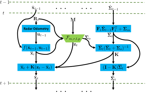
III-C Differentiable Kalman Filter
Kalman Filter is a general technique to fuse the sensor data in sequential. It consists of two steps, the prediction step using motion model and then followed by the updating step using measurement model, formulating a Bayesian recursive estimator with both models having Gaussian distributions.
Firstly, we propose an Iterative Closest Point (ICP) based radar odometry as the motion model, which estimates the relative pose between two timestamps i.e. from to . Specifically, radar points with high intensities are extracted from the raw data, and an intensity threshold is used to select salient points. Then ICP [46] is performed on these filtered points to estimate the pose. Based on this radar odometry, the prediction step of is formulated as follows:
| (8) |
where accumulates the ego-motion on the previous estimated pose, and is the Jacobian of . The predicted pose is calculated with the motion model in this equation. The covariance is also propagated and inserted with the odometry covariance , which is a pre-defined coefficient.
In the update step, we utilize the networks as the measurement model. We estimate the offset at the predicted location , then a global observation is generated by applying , where is the pose transformation process in Equation 1. With this GPS-like observation , we can derive the measurement model. We also calculate the observation covariance according to the probability distributions and derived above. Overall, the update step is formulated as follows:
| (9) |
where the , and stand for the Kalman gain, the estimated pose and the covariance respectively. The network aided KF system is presented in Figure 5. As both models are differentiable, the filter can be regarded as a recurrent network, which means that the measurement model can be trained by back-propagating gradients from future steps.
At the probabilistic perspective, KF generates the Gaussian posterior of the 3-dimensional pose in sequential, which is . Therefore, with the sequential ground truth pose available, we apply the maximum likelihood to tune the network parameters as follows:
| (10) |
where is the determinant of a matrix and we apply negative log-likelihood to formulate the minimization as
| (11) |
Based on the analysis, by discarding the constant terms, we can simply derive the third loss for end-to-end training of the sequential localization as
| (12) |
where is a constant balance factor, and denotes the length of sequence for training. This loss forms a balance between the likelihood and a lower uncertainty in the posterior.
III-D Implementation and Training Strategy
We implement the proposed RaLL using PyTorch [47], including networks at the front-end and KF at the back-end. The network architecture is presented in Appendix of this paper. As for the Differentiable Kalman Filter (DKF) proposed in Section III-C, it can be regarded as a block with feed-forward and back-propagation process. The whole system is trained on a single Nvidia Titan X GPU. As for the motion model, the ICP based radar odometry is implemented by using libpointmatcher [48].
We first train the measurement model using the single step loss . The training and test data is augmented by randomly sampling the initial poses near the ground truth poses. Furthermore, the pre-trained network is then trained with the sequential loss and differentiable Kalman Filter in an end-to-end manner, denoted as . The input data for training is sequences of temporal radar scans and corresponding ground truth poses. The performance tests with the trained and are presented in Section IV-B and IV-C.
IV Experiments
In Section IV-A, we first introduce the datasets for evaluation, then followed an ablation study in Section IV-B. The performance of pose tracking result is presented in Section IV-C, with comparisons to competitive methods. We also present the performance in dynamic environments in Section IV-D and the system operating efficiency in Section IV-E. Finally, the proposed measurement model is compared to recent localization methods with large inital offsets.
| Date | Len.(km) | Sequence |
|---|---|---|
| 10/01/2019 | 9.02 | Oxford-01: mapping & training |
| 10/01/2019 | 9.04 | Oxford-02: localization test |
| 11/01/2019 | 9.03 | Oxford-03: localization test |
| 16/01/2019 | 9.01 | Oxford-04: localization test |
| 17/01/2019 | 9.02 | Oxford-05: localization test |
| 18/01/2019 | 9.01 | Oxford-06: localization test |
| Date | Len.(km) | Sequence (Generalization) |
| 02/08/2019 | 4.91 | DCC-01: mapping & test |
| 23/08/2019 | 4.27 | DCC-02: localization test |
| 03/09/2019 | 5.42 | DCC-03: localization test |
| 20/06/2019 | 6.13 | KAIST-01: localization test |
| 23/08/2019 | 5.97 | KAIST-02: mapping & test |
| 02/09/2019 | 6.25 | KAIST-03: localization test |
| 02/08/2019 | 7.25 | Riverside-01: localization test |
| 16/08/2019 | 6.61 | Riverside-02: mapping & test |
IV-A Datasets
We conduct the experiments on the public autonomous driving datasets, Oxford Radar RobotCar (RobotCar)222https://oxford-robotics-institute.github.io/radar-robotcar-dataset [15, 16] in UK and Multimodal Range Dataset (MulRan)333https://sites.google.com/view/mulran-pr [17] in South Korea. Both of these datasets include ground truth poses, extrinsic calibration, raw lidar and radar data. The sensors types and locations on vehicles are different in the two datasets, thus validating the generalization of the proposed method indirectly.
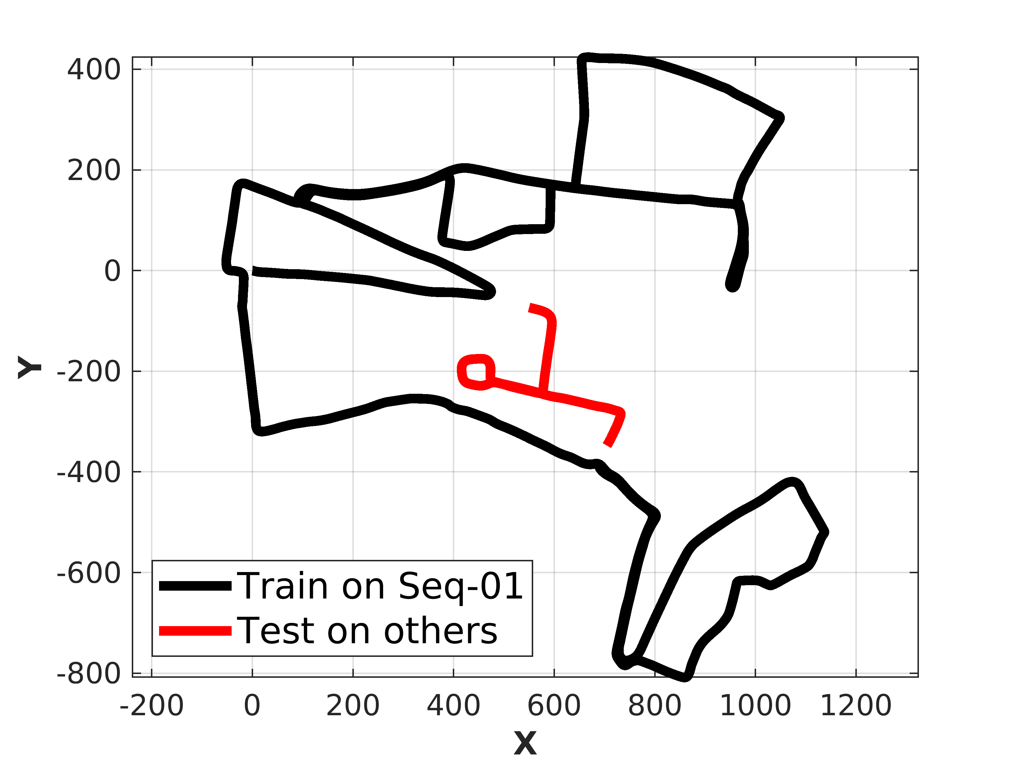
Table I and Table II present the details of the sequences in these two datasets. For RobotCar dataset, we select six sequences at different time, and Oxford-01 is used for mapping and network training. To validate RaLL in this paper, we follow the path split in [38], shown in Figure 7(a). As for MulRan dataset, sessions at DCC, KAIST and Riverside are used for evaluation. We build the laser maps using DCC-01, KAIST-02 and Riverside-02, and generalize all sequences directly using the learned model in RobotCar. This generalization strategy is performed in all the following experimental sections IV-B , IV-C and IV-F.
IV-B Ablation Study
| No. | Architecture | Mean Metric Error on RobotCar | Mean Metric Error on MulRan (Gen.) | ||||||
|---|---|---|---|---|---|---|---|---|---|
| DKF | (m) | (m) | (m) | (m) | |||||
| A | ✓ | 1.06 | 0.80 | 1.44 | 1.65 | 1.42 | 1.55 | ||
| B | ✓ | 1.71 | 1.03 | 2.06 | 2.09 | 2.33 | 2.24 | ||
| C | ✓ | ✓ | 1.05 | 0.74 | 1.55 | 1.62 | 1.40 | 1.59 | |
| D | ✓ | ✓ | ✓ | 1.04 | 0.69 | 1.26 | 1.67 | 1.37 | 1.40 |
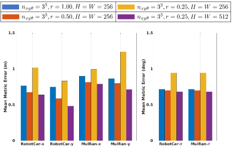
First of all, we employ the sensitivity analysis on the input range images, including the scan size and resolution . Input radar scans and lidar maps share four types of image settings, as shown in Figure 6(a); and then four networks are trained with these different inputs. The parameter varies when or relatively, thus guaranteeing the invariance of input patch sizes for the patch networks. The ablation study is manual labor consuming for training networks, but we consider it is worthy to explore an appropriate solution for radar localization.
We set the offset in the limit range as follows: , and , and also set the resolution in solution space, thus the cost volume is divided to . Samples are generated randomly with known offsets for training and evaluation. In RobotCar dataset, we collect more than 1000 samples in the test path of Oxford-02 and Oxford-03; and more than 3000 samples in DCC-02 and KAIST-02 of MulRan dataset. The estimated offset is inferenced by the trained networks . We calculate the mean errors of the estimated offsets alongside the three dimensions in robot coordinate.
The evaluation results are shown in Figure 6(a). It is obvious that the neural networks performs better than the others when and . And the network also works well with and . In summary, conclusions can be drawn from these comparisons: the higher range resolution is, or the longer detection range is, the more precise pose estimation will be achieved. But due to the constrained resources, it is a tradeoff between the image sizes and computing efficiency.
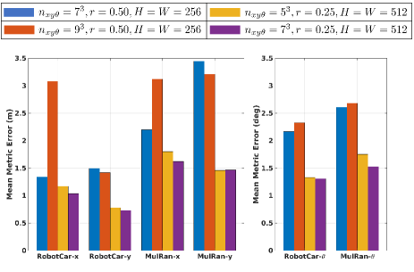
Based on the ablation results above, the best two settings and are selected for further tests. We extend the offset to , and . In this larger space, different resolutions are tested, resulting in and . Note that the difference of only cause changes of the patch network , in which the number of pose candidates is the number of channels essentially. As shown in Figure 6(b), it is obvious that the neural networks achieve best performance with and . The comparison between and when shows that higher resolution in offset space may not bring more precise estimation. We think it is because of the limited neurons in the network, which is hard to learn the distribution of a large number of possibilities.
| Method | Drift Trans. (%) | Rot. (deg/m) |
|---|---|---|
| VO Baseline [49] | 3.9802 | 0.0102 |
| UnDeepVO [50] | 4.7683 | 0.0141 |
| Cen RO [8] | 3.7168 | 0.0095 |
| Barnes RO [11] | 1.1627 | 0.0030 |
| Radar SLAM [13] | 2.1854 | 0.0071 |
| Fake-Lidar [39] | 4.1502 | 0.0119 |
| RaLL | 1.0933 | 0.0037 |
| Dataset | Mean Percentage of Relative Trans. (%) | |
|---|---|---|
| PhaRaO[12] | RaLL | |
| DCC-02 | 1.91 | 0.98 |
| Riverside-02 | 2.36 | 1.08 |
| Dataset | Mean Error of Relative Rot. (deg) | |
| PhaRaO[12] | RaLL | |
| DCC-02 | 2.34 | 2.03 |
| Riverside-02 | 4.66 | 1.98 |
Despite the analysis on the configuration paramters, we also conduct the ablation study of the network architectures. To achieve this, we remove or replace some blocks of the original system as follows:
-
•
: we test the performance with the removal of the masking network , and the radar and lidar feature generation processes are same in this context.
-
•
: we obtain the similarity scores without the patch division of , and difference scores are by applying the networks in Table LABEL:AblationNet.
-
•
DKF: we also test the performance with and without the differentiable Kalman Filter, which means the networks are trained with and respectively.
Table III shows the ablation study of blocks in system and the experimental results. First, No. C performs better than No. A and B, which demonstrates the effectiveness of the masking network and patch network . While compared to No. C, No. D is trained with DKF and achieves better performance, validating the superiority of differentiable Kalman Filter. In summary, we validate the effectiveness of our design with the ablation study of system architecture.
From these extensive ablation experiments, we also notice that the error in is generally larger than , which are longitudinal and lateral axes for automative vehicles relatively. We consider this result is interpretable due to the road environments in the two autonomous driving datasets. Most of the roads are straight for vehicles, and are more distinguishable along the lateral direction, especially when there are few features on the road sides. Therefore, it is more difficult to estimate the than in this paper.
| Sequence | Our RO | Fake-Lidar [39] | MCL () | RaLL () | RaLL () | |||||
|---|---|---|---|---|---|---|---|---|---|---|
| Trans.(m) | Rot.(∘) | Trans.(m) | Rot.(∘) | Trans.(m) | Rot.(∘) | Trans.(m) | Rot.(∘) | Trans.(m) | Rot.(∘) | |
| Oxford-02 | 263.27 | 26.93 | 8.46 | 5.43 | 2.96 | 1.89 | 1.42 | 1.53 | 0.98 | 1.45 |
| Oxford-03 | 229.95 | 17.04 | 6.93 | 2.46 | 3.09 | 1.92 | 1.65 | 1.66 | 1.14 | 1.62 |
| Oxford-04 | 131.66 | 11.16 | 9.12 | 4.47 | 3.24 | 2.02 | 2.18 | 2.00 | 1.71 | 1.93 |
| Oxford-05 | 439.23 | 44.14 | - | - | 2.93 | 1.89 | 1.47 | 1.57 | 1.11 | 1.48 |
| Oxford-06 | 333.04 | 19.45 | 14.10 | 4.25 | 2.96 | 1.97 | 1.52 | 1.57 | 1.14 | 1.52 |
| RobotCar-all | 303.17 | 27.03 | 10.06 | 4.33 | 3.04 | 1.94 | 1.66 | 1.67 | 1.23 | 1.60 |
| DCC-01 | 218.47 | 51.41 | - | - | 377.08 | 106.25 | 2.90 | 2.01 | 2.11 | 1.97 |
| DCC-02 | 96.96 | 21.90 | - | - | 730.07 | 92.45 | 5.10 | 2.28 | 4.71 | 2.01 |
| DCC-03 | 146.28 | 33.64 | - | - | 7.30 | 2.78 | 5.88 | 2.75 | 5.14 | 2.55 |
| KAIST-01 | 376.97 | 65.04 | - | - | 3.36 | 2.06 | 1.98 | 1.88 | 1.45 | 1.74 |
| KAIST-02 | 216.47 | 47.43 | - | - | 3.37 | 1.99 | 1.86 | 1.79 | 1.30 | 1.71 |
| KAIST-03 | 242.72 | 39.56 | - | - | 3.13 | 2.00 | 1.97 | 1.60 | 1.27 | 1.50 |
| Riverside-01 | 367.30 | 39.61 | - | - | 939.15 | 109.86 | 497.82 | 48.09 | 4.12 | 2.84 |
| Riverside-02 | 407.65 | 32.04 | - | - | 1245.66 | 81.55 | 9.52 | 3.19 | 2.52 | 1.93 |
| MulRan-all | 275.61 | 41.49 | - | - | 610.13 | 64.34 | 151.35 | 14.77 | 3.12 | 2.02 |
| All sequence | 293.30 | 33.11 | - | - | 370.42 | 39.09 | 91.90 | 9.09 | 2.13 | 1.77 |
| Sequence | Our RO | Fake-Lidar [39] | MCL () | RaLL () | RaLL () | |||||
|---|---|---|---|---|---|---|---|---|---|---|
| Trans.(m) | Rot.(∘) | Trans.(m) | Rot.(∘) | Trans.(m) | Rot.(∘) | Trans.(m) | Rot.(∘) | Trans.(m) | Rot.(∘) | |
| Oxford-02 | 150.61 | 19.49 | 1.53 | 1.10 | 2.54 | 1.03 | 1.07 | 0.46 | 0.65 | 0.40 |
| Oxford-03 | 207.20 | 14.58 | 1.38 | 1.16 | 2.55 | 1.06 | 1.22 | 0.51 | 0.79 | 0.49 |
| Oxford-04 | 100.48 | 8.66 | 2.05 | 1.32 | 2.67 | 1.17 | 1.62 | 0.73 | 1.14 | 0.68 |
| Oxford-05 | 269.91 | 37.77 | - | - | 2.50 | 1.10 | 1.05 | 0.59 | 0.71 | 0.56 |
| Oxford-06 | 283.61 | 16.67 | 2.04 | 1.51 | 2.46 | 1.09 | 1.03 | 0.40 | 0.88 | 0.43 |
| RobotCar-all | 182.73 | 15.77 | 1.70 | 1.25 | 2.54 | 1.09 | 1.17 | 0.53 | 0.80 | 0.50 |
| DCC-01 | 159.41 | 45.70 | - | - | 358.85 | 103.19 | 2.29 | 1.02 | 1.38 | 0.97 |
| DCC-02 | 92.15 | 20.33 | - | - | 705.12 | 68.83 | 4.63 | 0.88 | 4.38 | 0.80 |
| DCC-03 | 92.46 | 36.25 | - | - | 5.72 | 1.60 | 5.24 | 1.54 | 4.45 | 1.40 |
| KAIST-01 | 305.38 | 47.35 | - | - | 2.86 | 1.26 | 1.70 | 1.01 | 1.12 | 0.93 |
| KAIST-02 | 128.97 | 23.22 | - | - | 2.79 | 1.17 | 1.57 | 0.86 | 1.05 | 0.83 |
| KAIST-03 | 174.33 | 27.26 | - | - | 2.67 | 1.24 | 1.72 | 0.87 | 0.99 | 0.80 |
| Riverside-01 | 185.04 | 31.17 | - | - | 745.98 | 99.36 | 4.76 | 1.63 | 2.87 | 1.32 |
| Riverside-02 | 166.81 | 23.52 | - | - | 323.36 | 29.40 | 2.86 | 1.33 | 2.15 | 1.05 |
| MulRan-all | 141.26 | 27.93 | - | - | 5.77 | 2.45 | 2.37 | 1.07 | 1.65 | 0.97 |
| All sequence | 168.78 | 18.97 | - | - | 3.02 | 1.37 | 1.52 | 0.68 | 1.01 | 0.65 |
IV-C Pose Tracking Evaluation
For the following experiments in Section IV-C, IV-D, IV-E and IV-F, we use the best configuration from the ablation study above: , and the volume is set as for estimation in , and also the proposed differentiable system in this paper.
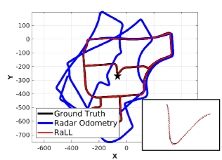
First, our proposed RaLL is compared to other competitive methods on RobotCar dataset. We follow the experiment settings in [11] and [13], in which the localization precisions were calculated under the odometry evaluation of KITTI benchmarking [51]. Specifically, the errors equal to the mean translation and rotation errors from 100 to 800 with the incremental distance travalled. We use the open source tool 444https://github.com/Huangying-Zhan/kitti-odom-eval [52] for odometic error calculation on sub-seqeuences.
These competitive methods include the visual odometry based merthods [49, 50], RO [8, 11] and RadarSLAM [13]. The results are presented in Table IV, in which RaLL achieves the best performance on translation error evaluation, thus validating the effectiveness of the differentiable measurement model and differentiable KF in this paper.
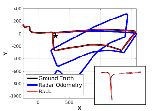
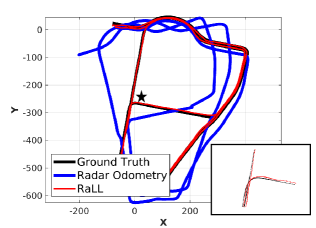
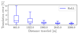
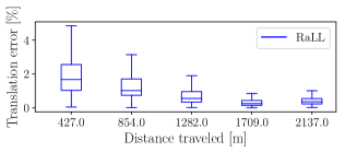
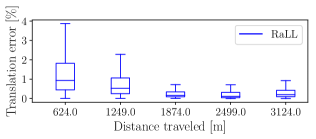
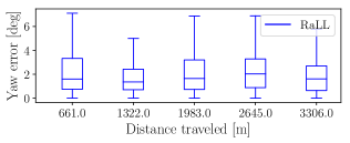
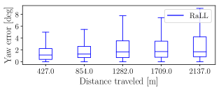
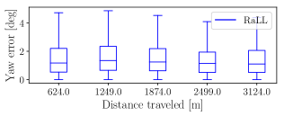
To achieve the extensive comparisons, we also comapre the RaLL with the direct radar odometry PhaRaO [12]. We follow the experiment settings in [12], in which the relative errors were computed with the evaluation tool 555https://github.com/uzh-rpg/rpg_trajectory_evaluation in [53]. In this context, the relative errors are presented in Figure 8 with the mean values in Table V. Our proposed RaLL performs better than PhaRaO on MulRan dataset though the learned model is trained on RobotCar dataset.
We also calculate the absolute trajectory errors on the whole trajectories. Our proposed radar odometry (RO) is selected as a comparison for evaluation. Furthermore, our previous work [39] used GAN to transform radar to fake lidar representations, and MCL was constructed with overlap based mearsurement model. We denote this method as Fake-Lidar. Based on this MCL framework, we also use the differentiable measurement model in this paper for pose tracking, which is denoted as MCL(). In addition, the particle filter is updated to KF in this paper, which is the proposed RaLL() as a comparison. Finally, the complete RaLL with the () is performed, which is trained with the supervision of differentiable Kalman Filter.
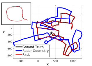
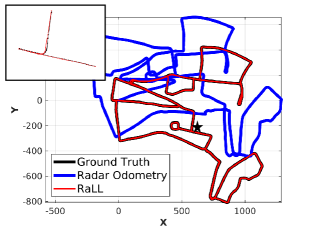
As shown in Table VI and VII, both the Root Mean Squared Errors (RMSE) and median errors of each sequence are calculated with the comparison to the ground truth poses, and we also present the results of the whole dataset. It is obvious that the RaLL() achieves the best performance over the 90 driving. Several localization trajectries are presented in Figure 7 and 8 with the zoomed views.
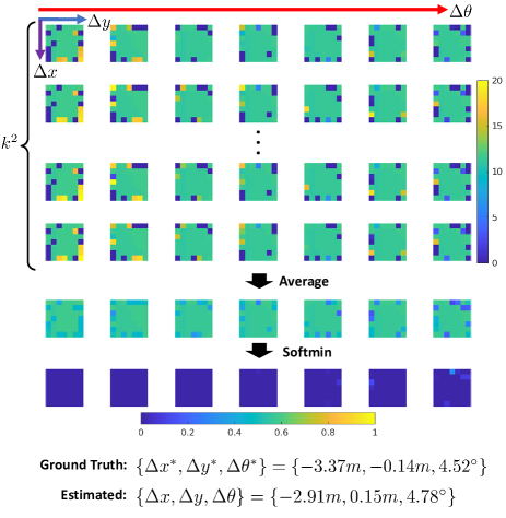
Figure 9 presents a case study on the result in visualization. The resulting tensor size from the patch network is , and we formulate it to axes for better visualization. After averaging of tensors and softmin operation, the differences are transfomed to the offset probabilities in the range of . Finally, the estimated pose offset is close to the ground truth for pose tracking, and the visualization results demonstrate that our proposed networks have good interpretability.
IV-D Performance in Dynamic Environments
Despite the comparisons and evaluations across the whole trajectories, we also investigate the localization performance in dynamic environments. Actually, there are various dynamic objects in both RobotCar and Mulran dataset, including the moving vehicles, bicycles and pedestrians etc. Our proposed RaLL runs successfully in the 90 drives without any localization failure, thus indicating the feasibility of RaLL in dynamic environments.
To better explore the effects of dynamics, we present the peformance in two case studies of Oxford-02, as shown in Figure 10. Obviously, there are moving objects in the streets and crossings, which have negative effects on our localization precision. However, the RaLL finally corrects the vehicles within limited driving distance. We consider there are two main reasons as follows: first, different from the dynamics in vision [22, 23] and lidar [54, 17], radar sensor suffers less from the object occlusions; second, the proposed measurement model contains the convolution and pooling layers, leading to limited impacts of dynamics in feature embeddings. In summary, our proposed system could be able to handle the dynamics and provide acceptable localization results in dynamical urban scenes.
| Module | Our RO | KF | Total | |
|---|---|---|---|---|
| Time(ms) | 92.78 | 28.90 | 122.19 | 243.87 |
| Methods | Device | Freq.(Hz) |
|---|---|---|
| Rapp RO [31] | Intel i7-5930K CPU | 17 |
| Map Recon. [27] | Nvidia Jetson TX2 | 1.54 |
| Cen RO [8] | / | 3 |
| Barnes RO [11] | Nvidia Titan Xp GPU | 13.4 |
| PhaRaO [12] | Intel i7-7700K CPU | 10.73 |
| Radar SLAM [13] | Intel i7 CPU | 6 |
| Our RO | Intel Xeon E7 | 10.78 |
| RaLL | Nvidia Titan X GPU | 4.11 |
IV-E Efficiency Evaluation
To access the time costs of our proposed radar localization system, we measure the computation efficiency on Oxford-02. More than 8600 radar images are fed into our system and the average time cost of each module is presented in Table VIII. The total time cost for every inference is 243.87, and the whole system runs at 4.11 Hz on average. Since the Navtech FMCW radar is operating at 4 Hz, our proposed RaLL achives the real-time performance.
Despite the efficiency analysis of RaLL, we investigate the time costs of other recent research works. Some works are based on learning methods and some are not, leading to the differences on computing devices, so we also list the main computing devices in these papers, as shown in Table IX. In addition, some other factors also affect the efficiencies, system implementations and radar resolutions etc, and the final algorithm efficiency may vary in practical applications.
Limitation For vehicle localization in real world, we consider the transplanting to embedded platform is critically important. The proposed model is deployed on a powerful GPU in this paper, which is an obvious limitation of our proposed RaLL. To overcome this, there are several feasible ways to improve the operating efficiency, such as neural architecture optimization and multi-gpu parallel programming etc.
IV-F Localization with the Large Offsets
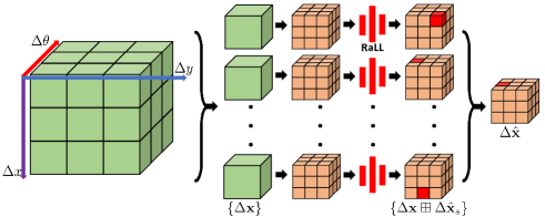
To make more extensive comparisons, we also perform the localization with large initial offset same as [37, 38], which evaluates the measurement model directly in this paper. For a fair comparison, we expand the solution space to , which is close to the experiments in [37, 38], and is also a very large offset on pixel levels in this paper. More than 200 and 500 samples are generated in the test path of Oxford-02 and KAIST-02.
However, our proposed network is designed for limited offsets originally, and not applicable to large offsets. To achieve this goal, we divide the entire space to several sub-spaces, illustrated in Figure 11. And initial guesses are raised in the center of these sub-spaces as initial offsets . Then the proposed network is applied at each initial offset, and we can obtain the estimated in sub-spaces. While in the entire space, all the potential solutions are , where is the pose transformation process in Equation 1, and the problem is then transformed to find the best solution in this answer set. In Section III-B, a coarse similarity is measured by subtraction of embedding, and here we calculate this similarity to select the best sub-space directly. Finally, in , we regard the offset with highest similarity as the estimated offset .
The evaluation results are presented in Table X, and we exchange and in [37, 38] because of the different representations in methodologies. Our proposed method performs better overall the performance, compared to another two deep learning based methods. This experiment indicates that our network not only handles long-term pose tracking, but also the localization with large offsets.
V Conclusion
An end-to-end system RaLL is proposed in this paper, which can localize a rotating radar sensor on a prior lidar map. To achieve this, we first build networks to extract comparable embeddings of different sensor modalities, and then form the pose probabilities via differentiable solver. The Kalman Filter is applied to model the measurement uncertainty in end-to-end manner, and also fuse the measurement and motion for pose tracking. In multi-session multi-scene datasets, we demonstrate the effectiveness of the proposed differentiable localization system, with the comparison to other competitive methods.
On the other hand, there remain some promising directions to overcome the limitations. First, the code transplanting to embedded platform is important for practical applications, and several feasible solutions are expected to improve the operating efficiency, e.g. the multi-core parallel programming. Second, based on the existing end-to-end visual odometry [50] and lidar odometry [55], we intend to develop the uncertainty modeling of the radar odometry. Finally, the optimal network model is critical in real applications, which improves both effectiveness and efficiency for deployment, and we consider that the Neural Architecture Search (NAS) [56] can explore the best solution of our network design in the future.
Appendix A Network Architecture
For the feature embedding network, we follow the general settings in relative works [11, 38, 36]. As for the proposed patch network, we set the input image sizes as for experiments. The abbreviations and network architectures are as follows:
-
•
D-Net(): A doubled neural network in U-Net
-
•
Conv(): convolution on 2D image with input channels, output channels, kernel size , stride , and padding
-
•
IN: instance normalization
-
•
BN: batch normalization
-
•
ReLU: rectified linear unit function
-
•
Pool(): max pooling with kernel size , stride and padding
-
•
UpSampling(): upsample on 2D image with a scale factor
-
•
Skip: skip connection between layers
The network architectures are shown in Table LABEL:DoubleNet, Table LABEL:UNet and Table LABEL:PatchNet, and Table LABEL:AblationNet presents the structure for training without the patch network.
| Conv(,,3,1,1) + IN + ReLU |
| Conv(,,3,1,1) + IN + ReLU |
| D-Net(1,8,8) + Pool(2,2,0) |
| D-Net(8,16,16) + Pool(2,2,0) |
| D-Net(16,32,32) + Pool(2,2,0) |
| D-Net(32,64,64) + Pool(2,2,0) |
| D-Net(64,64,64) |
| UpSamping(2) + Skip + D-Net(128,64,32) |
| UpSamping(2) + Skip + D-Net(64,32,16) |
| UpSamping(2) + Skip + D-Net(32,16,8) |
| UpSamping(2) + Skip + D-Net(16,8,8) |
| : Conv(8,1,1,1,0) + Sigmoid |
| : Conv(8,1,3,1,0) + IN + ReLU |
| : Conv(8,1,3,1,0) + IN + ReLU |
| Conv(,,4,2,1) + BN + ReLU 3 |
| Conv(,,4,1,0) + BN + ReLU |
| Conv(,,4,2,1) + BN + ReLU 7 |
| Conv(,,4,1,0) + ReLU |
References
- [1] R. Mur-Artal, J. M. M. Montiel, and J. D. Tardos, “Orb-slam: a versatile and accurate monocular slam system,” IEEE transactions on robotics, vol. 31, no. 5, pp. 1147–1163, 2015.
- [2] X. Ding, Y. Wang, R. Xiong, D. Li, L. Tang, H. Yin, and L. Zhao, “Persistent stereo visual localization on cross-modal invariant map,” IEEE Transactions on Intelligent Transportation Systems, 2019.
- [3] P. Krüsi, B. Bücheler, F. Pomerleau, U. Schwesinger, R. Siegwart, and P. Furgale, “Lighting-invariant adaptive route following using iterative closest point matching,” Journal of Field Robotics, vol. 32, no. 4, pp. 534–564, 2015.
- [4] E. Javanmardi, M. Javanmardi, Y. Gu, and S. Kamijo, “Pre-estimating self-localization error of ndt-based map-matching from map only,” IEEE Transactions on Intelligent Transportation Systems, 2020.
- [5] W. Lu, Y. Zhou, G. Wan, S. Hou, and S. Song, “L3-net: Towards learning based lidar localization for autonomous driving,” in Proceedings of the IEEE Conference on Computer Vision and Pattern Recognition, 2019, pp. 6389–6398.
- [6] I. A. Barsan, S. Wang, A. Pokrovsky, and R. Urtasun, “Learning to localize using a lidar intensity map.” in Conference on Robot Learning (CoRL), 2018, pp. 605–616.
- [7] A. Carballo, J. Lambert, A. Monrroy, D. Wong, P. Narksri, Y. Kitsukawa, E. Takeuchi, S. Kato, and K. Takeda, “Libre: The multiple 3d lidar dataset,” in 2020 IEEE Intelligent Vehicles Symposium (IV). IEEE, 2020.
- [8] S. H. Cen and P. Newman, “Precise ego-motion estimation with millimeter-wave radar under diverse and challenging conditions,” in 2018 IEEE International Conference on Robotics and Automation (ICRA). IEEE, 2018, pp. 1–8.
- [9] ——, “Radar-only ego-motion estimation in difficult settings via graph matching,” in 2019 International Conference on Robotics and Automation (ICRA). IEEE, 2019, pp. 298–304.
- [10] R. Aldera, D. De Martini, M. Gadd, and P. Newman, “Fast radar motion estimation with a learnt focus of attention using weak supervision,” in 2019 International Conference on Robotics and Automation (ICRA). IEEE, 2019, pp. 1190–1196.
- [11] D. Barnes, R. Weston, and I. Posner, “Masking by moving: Learning distraction-free radar odometry from pose information,” in Conference on Robot Learning (CoRL), 2020, pp. 303–316.
- [12] Y. S. Park, Y.-S. Shin, and A. Kim, “Pharao: Direct radar odometry using phase correlation,” in IEEE International Conference on Robotics and Automation (ICRA), 2020.
- [13] Z. Hong, Y. Petillot, and S. Wang, “Radarslam: Radar based large-scale slam in all weathers,” in 2020 IEEE/RSJ International Conference on Intelligent Robots and Systems (IROS), 2020.
- [14] W.-C. Ma, I. Tartavull, I. A. Bârsan, S. Wang, M. Bai, G. Mattyus, N. Homayounfar, S. K. Lakshmikanth, A. Pokrovsky, and R. Urtasun, “Exploiting sparse semantic hd maps for self-driving vehicle localization,” pp. 5304–5311, 2019.
- [15] D. Barnes, M. Gadd, P. Murcutt, P. Newman, and I. Posner, “The oxford radar robotcar dataset: A radar extension to the oxford robotcar dataset,” arXiv preprint arXiv: 1909.01300, 2019.
- [16] W. Maddern, G. Pascoe, C. Linegar, and P. Newman, “1 year, 1000 km: The oxford robotcar dataset,” The International Journal of Robotics Research, vol. 36, no. 1, pp. 3–15, 2017.
- [17] G. Kim, Y. S. Park, Y. Cho, J. Jeong, and A. Kim, “Mulran: Multimodal range dataset for urban place recognition,” in IEEE International Conference on Robotics and Automation (ICRA), 2020.
- [18] G. Ros, A. Sappa, D. Ponsa, and A. M. Lopez, “Visual slam for driverless cars: A brief survey,” in Intelligent Vehicles Symposium (IV) Workshops, vol. 2, 2012.
- [19] T. Akilan, E. Johnson, G. Taluja, J. Sandhu, and R. Chadha, “Multimodality weight and score fusion for slam,” in 2020 IEEE Canadian Conference on Electrical and Computer Engineering (CCECE). IEEE, pp. 1–4.
- [20] X. Ding, Y. Wang, H. Yin, L. Tang, and R. Xiong, “Multi-session map construction in outdoor dynamic environment,” in 2018 IEEE International Conference on Real-time Computing and Robotics (RCAR). IEEE, 2018, pp. 384–389.
- [21] G. Bresson, Z. Alsayed, L. Yu, and S. Glaser, “Simultaneous localization and mapping: A survey of current trends in autonomous driving,” IEEE Transactions on Intelligent Vehicles, vol. 2, no. 3, pp. 194–220, 2017.
- [22] Y. Sun, M. Liu, and M. Q.-H. Meng, “Improving rgb-d slam in dynamic environments: A motion removal approach,” Robotics and Autonomous Systems, vol. 89, pp. 110–122, 2017.
- [23] ——, “Motion removal for reliable rgb-d slam in dynamic environments,” Robotics and Autonomous Systems, vol. 108, pp. 115–128, 2018.
- [24] H. Huang, H. Ye, Y. Sun, and M. Liu, “Gmmloc: Structure consistent visual localization with gaussian mixture models,” IEEE Robotics and Automation Letters, vol. 5, no. 4, pp. 5043–5050, 2020.
- [25] H. Yin, Y. Wang, X. Ding, L. Tang, S. Huang, and R. Xiong, “3d lidar-based global localization using siamese neural network,” IEEE Transactions on Intelligent Transportation Systems, vol. 21, no. 4, pp. 1380–1392, 2019.
- [26] Y. S. Park, J. Kim, and A. Kim, “Radar localization and mapping for indoor disaster environments via multi-modal registration to prior lidar map,” in 2019 IEEE/RSJ International Conference on Intelligent Robots and Systems (IROS). IEEE, 2019, pp. 1307–1314.
- [27] C. X. Lu, S. Rosa, P. Zhao, B. Wang, C. Chen, J. A. Stankovic, N. Trigoni, and A. Markham, “See through smoke: robust indoor mapping with low-cost mmwave radar.” in MobiSys, 2020, pp. 14–27.
- [28] D. Vivet, P. Checchin, and R. Chapuis, “Localization and mapping using only a rotating fmcw radar sensor,” Sensors, vol. 13, no. 4, pp. 4527–4552, 2013.
- [29] F. Schuster, M. Wörner, C. G. Keller, M. Haueis, and C. Curio, “Robust localization based on radar signal clustering,” in 2016 IEEE Intelligent Vehicles Symposium (IV). IEEE, 2016, pp. 839–844.
- [30] F. Schuster, C. G. Keller, M. Rapp, M. Haueis, and C. Curio, “Landmark based radar slam using graph optimization,” in 2016 IEEE 19th International Conference on Intelligent Transportation Systems (ITSC). IEEE, 2016, pp. 2559–2564.
- [31] M. Rapp, M. Barjenbruch, M. Hahn, J. Dickmann, and K. Dietmayer, “Probabilistic ego-motion estimation using multiple automotive radar sensors,” Robotics and Autonomous Systems, vol. 89, pp. 136–146, 2017.
- [32] L. Narula, P. A. Iannucci, and T. E. Humphreys, “Automotive-radar-based 50-cm urban positioning,” in 2020 IEEE/ION Position, Location and Navigation Symposium (PLANS). IEEE, 2020, pp. 856–867.
- [33] K. Burnett, A. P. Schoellig, and T. D. Barfoot, “Do we need to compensate for motion distortion and doppler effects in radar-based navigation?” arXiv preprint arXiv:2011.03512, 2020.
- [34] M. Gadd, D. De Martini, and P. Newman, “Look around you: Sequence-based radar place recognition with learned rotational invariance,” in 2020 IEEE/ION Position, Location and Navigation Symposium (PLANS). IEEE, 2020, pp. 270–276.
- [35] Ş. Săftescu, M. Gadd, D. De Martini, D. Barnes, and P. Newman, “Kidnapped radar: Topological radar localisation using rotationally-invariant metric learning,” in IEEE International Conference on Robotics and Automation (ICRA), 2020.
- [36] D. Barnes and I. Posner, “Under the radar: Learning to predict robust keypoints for odometry estimation and metric localisation in radar,” in IEEE International Conference on Robotics and Automation (ICRA), 2020.
- [37] T. Y. Tang, D. De Martini, D. Barnes, and P. Newman, “Rsl-net: Localising in satellite images from a radar on the ground,” IEEE Robotics and Automation Letters, vol. 5, no. 2, pp. 1087–1094, 2020.
- [38] T. Y. Tang, D. De Martini, S. Wu, and P. Newman, “Self-supervised localisation between range sensors and overhead imagery,” in Robotics: Science and Systems (RSS), 2020.
- [39] H. Yin, Y. Wang, L. Tang, and R. Xiong, “Radar-on-lidar: metric radar localization on prior lidar maps,” in 2020 IEEE International Conference on Real-time Computing and Robotics (RCAR). IEEE, 2020, best Conference Paper Award.
- [40] H. Yin, Y. Wang, L. Tang, X. Ding, S. Huang, and R. Xiong, “3d lidar map compression for efficient localization on resource constrained vehicles,” IEEE Transactions on Intelligent Transportation Systems, 2020.
- [41] H. Huang, H. Ye, Y. Sun, and M. Liu, “Monocular visual odometry using learned repeatability and description,” in 2020 IEEE International Conference on Robotics and Automation (ICRA). IEEE, 2020, pp. 8913–8919.
- [42] C. Chen, B. Wang, C. X. Lu, N. Trigoni, and A. Markham, “A survey on deep learning for localization and mapping: Towards the age of spatial machine intelligence,” arXiv preprint arXiv:2006.12567, 2020.
- [43] A. Kendall, M. Grimes, and R. Cipolla, “Posenet: A convolutional network for real-time 6-dof camera relocalization,” in Proceedings of the IEEE international conference on computer vision, 2015, pp. 2938–2946.
- [44] D. DeTone, T. Malisiewicz, and A. Rabinovich, “Superpoint: Self-supervised interest point detection and description,” in Proceedings of the IEEE Conference on Computer Vision and Pattern Recognition Workshops, 2018, pp. 224–236.
- [45] O. Ronneberger, P. Fischer, and T. Brox, “U-net: Convolutional networks for biomedical image segmentation,” in International Conference on Medical image computing and computer-assisted intervention. Springer, 2015, pp. 234–241.
- [46] P. J. Besl and N. D. McKay, “Method for registration of 3-d shapes,” in Sensor fusion IV: control paradigms and data structures, vol. 1611. International Society for Optics and Photonics, 1992, pp. 586–606.
- [47] A. Paszke, S. Gross, F. Massa, A. Lerer, J. Bradbury, G. Chanan, T. Killeen, Z. Lin, N. Gimelshein, L. Antiga et al., “Pytorch: An imperative style, high-performance deep learning library,” in Advances in neural information processing systems, 2019, pp. 8026–8037.
- [48] F. Pomerleau, F. Colas, R. Siegwart, and S. Magnenat, “Comparing icp variants on real-world data sets,” Autonomous Robots, vol. 34, no. 3, pp. 133–148, 2013.
- [49] W. S. Churchill, “Experience based navigation: Theory, practice and implementation,” 2012.
- [50] R. Li, S. Wang, Z. Long, and D. Gu, “Undeepvo: Monocular visual odometry through unsupervised deep learning,” in 2018 IEEE international conference on robotics and automation (ICRA). IEEE, 2018, pp. 7286–7291.
- [51] A. Geiger, P. Lenz, and R. Urtasun, “Are we ready for autonomous driving? the kitti vision benchmark suite,” in Conference on Computer Vision and Pattern Recognition (CVPR), 2012.
- [52] H. Zhan, C. S. Weerasekera, J. Bian, and I. Reid, “Visual odometry revisited: What should be learnt?” in 2020 IEEE International Conference on Robotics and Automation (ICRA). IEEE, 2020.
- [53] Z. Zhang and D. Scaramuzza, “A tutorial on quantitative trajectory evaluation for visual (-inertial) odometry,” in 2018 IEEE/RSJ International Conference on Intelligent Robots and Systems (IROS). IEEE, 2018, pp. 7244–7251.
- [54] H. Yin, X. Ding, L. Tang, Y. Wang, and R. Xiong, “Efficient 3d lidar based loop closing using deep neural network,” in 2017 IEEE International Conference on Robotics and Biomimetics (ROBIO). IEEE, 2017, pp. 481–486.
- [55] Q. Li, S. Chen, C. Wang, X. Li, C. Wen, M. Cheng, and J. Li, “Lo-net: Deep real-time lidar odometry,” in Proceedings of the IEEE Conference on Computer Vision and Pattern Recognition, 2019, pp. 8473–8482.
- [56] T. Elsken, J. H. Metzen, F. Hutter et al., “Neural architecture search: A survey.” J. Mach. Learn. Res., vol. 20, no. 55, pp. 1–21, 2019.