Engineered Swift Equilibration of a Brownian Gyrator

Abstract

In the context of stochastic thermodynamics, a minimal model for non equilibrium steady states has been recently proposed: the Brownian Gyrator (BG). It describes the stochastic overdamped motion of a particle in a two dimensional harmonic potential, as in the classic Ornstein-Uhlenbeck process, but considering the simultaneous presence of two independent thermal baths. When the two baths have different temperatures, the steady BG exhibits a rotating current, a clear signature of non equilibrium dynamics. Here, we consider a time-dependent potential, and we apply a reverse-engineering approach to derive exactly the required protocol to switch from an initial steady state to a final steady state in a finite time $\tau$. The protocol can be built by first choosing an arbitrary quasi-static counterpart - with few constraints - and then adding a finite-time contribution which only depends upon the chosen quasi-static form and which is of order $1/\tau$. We also get a condition for transformations which - in finite time - conserve internal energy, useful for applications such as the design of microscopic thermal engines. Our study extends finite-time stochastic thermodynamics to transformations connecting non-equilibrium steady states.

Introduction - Fast switching through two or more modes of operation in microscopic experiments - where fluctuations dominate - is a goal for several applications: cyclical mesoscopic thermal machines such as colloids in time-dependent optical traps Blickle and Bechinger (2012); Martinez et al. (2015); Schmiedl and Seifert (2007); Bo and Celani (2013); Martinez et al. (2016a); Quinto-Su (2014), thermal engines realised in bacterial baths Krishnamurthy et al. (2016); Di Leonardo et al. (2010), realisation of bit operation under noisy environment with connection to information theory Bérut et al. (2012) and much more. Experiments and theory have recently demonstrated the existence of special protocols that in finite time realise conditions which are usually realised in infinite time: these protocols can be deduced by reverse-engineering the desired, fast, path of evolution of given observables, including the probability distribution in phase space Guéry-Odelin et al. (2019, 2014).

A paradygmatic example has been given in one effective dimension with a harmonic trap, realised by optical radiation confining a colloidal particle Martinez et al. (2016b). The colloidal particle has reached a steady state in the trap with a stiffness $k^{i}$. Then the trap is modulated from the initial stiffness $k^{i}$ to a new stiffness $k^{f}$ in some finite time $\tau$. If the change $k^{i}\to k^{f}$ is realised in too short a time, e.g. taking ideally $\tau=0$ (what is called “STEP” protocol), then the colloidal particle will take some uncontrolled additional time to reach the steady state compatible with the final stiffness. Such a “natural” time is related to the typical relaxation times of the system and can be very long, depending upon the situations. Interestingly, it is possible to design one or more “swift equilibration” (SE) protocols $k(t)$, with $k(0)=k^{i}$ and $k(\tau)=k^{f}$, such that at time $\tau$ the final steady state is reached and no additional relaxation time is needed. The shape of $k(t)$ can be non-intuitive: when $\tau$ is smaller than the typical relaxation times, such protocols may exhibit large excursions well outside of the range $[k^{i},k^{f}]$. In fact, there are cases where $k(t)$ can even become negative, posing problems to its experimental realization. Additional constraints may be introduced into the mathematical design problem, in order to limit the protocol excursion Plata et al. (2019). Other possibilities have been suggested, where the trap position is also modulated by additional noise Chupeau et al. (2018a). The SE protocol has been demonstrated also in an atomic force microscopy experiments Le Cunuder et al. (2016).

Here, we discuss the problem of swift equilibration in a two-dimensional harmonic trap. The generalization may seem a pure increase of dimensionality, but in fact it allows us to step outside of the realm of pure equilibrium steady states. A two-dimensional harmonic trap may be coupled to different thermostats and, in general, may exhibit rotating currents which break the time-reversal symmetry even in the steady state Ciliberto et al. (2013); Filliger and Reimann (2007); Dotsenko et al. (2013); Cerasoli et al. (2018); Villamaina et al. (2009); Argun et al. (2017); Chiang et al. (2017); Soni et al. (2017). It is therefore a sound test-ground for the study of SE protocols for switching between two different non-equilibrium steady states in a finite time.

Swift equilibration protocol - Firstly, let us introduce the general strategy for the SE. We adopted a different and, in a sense, more general approach with respect to Martinez et al. (2016b). Consider an experimental system that can be leveraged controlling some forcing parameters, which will be noted in a vector ${\mathbf{\Pi}}$. The instantaneous statistical state of the system can be described by a set of parameters, which will be denoted by a vector $\bm{\gamma}(t)$: for instance in a Gaussian process, as in our case below, these can be the parameters of a multivariate Gaussian. The value of the parameters $\bm{\gamma}(t)$ depends, through a dynamical equation, on the the history of the applied forcing ${\mathbf{\Pi}}$ up to time $t$. We prepare the system in a stationary condition, given a value for the forcing ${\mathbf{\Pi}}^{i}$. This means that we observe a time constant value of the system parameters $\bm{\gamma}$ that depends on the forcing ${\mathbf{\Pi}}^{i}$: we note this value as $\bm{\gamma}^{st}[{\mathbf{\Pi}}^{i}]$. Our goal is to lead the system into a new stationary state with a final set of parameters $\bm{\gamma}^{st}[{\mathbf{\Pi}}^{f}]$, in a finite time $\tau$.

Of course, if $\tau$ is very large, any transformation behaves as a SE protocol. More precisely, let us consider an arbitrary function ${\mathbfcal{P}}(s)$, with $s\in[0,1]$, such that ${\mathbfcal{P}}(0)={\mathbf{\Pi}}^{i}$ and ${\mathbfcal{P}}(1)={\mathbf{\Pi}}^{f}$. Then the evolution of parameters ${\mathbf{\Pi}}(t)={\mathbfcal{P}}(t/\tau)$ is a SE protocol in the limit $\tau$ much larger than the largest characteristic time of the system dynamics. In fact in this case the change in the forcing parameters is so slow that the system is always in its stationary state. In this quasi-static forcing, $\bm{\gamma}(t)=\bm{\gamma}^{st}[{\mathbfcal{P}}(t/\tau)]$ at any time, including the final one.

On the contrary, when $\tau$ is finite (smaller than the largest characteristic time of the system), ${\mathbfcal{P}}(t/\tau)$ is not a SE and must be modified with appropriate finite time corrections, i.e. a finite-$\tau$ SE protocol reads ${\mathbf{\Pi}}={\mathbfcal{P}}+\frac{1}{\tau}\delta{\mathbfcal{P}}$: here we denote the finite time corrections with $\delta{\mathbfcal{P}}$. The quantity $\delta{\mathbfcal{P}}$ , hereafter named the finite time correction to the quasi-static protocol, depends upon the choice of the quasi-static protocol ${\mathbfcal{P}}$. This is the relevant quantity one has to know to experimentally perform the desired SE. The exact, explicit and general formula for $\delta{\mathbfcal{P}}[{\mathbfcal{P}}(s)]$ in the case of the Brownian Gyrator constitutes the main result of this letter, and it allows a number of interesting theoretical considerations.

The Brownian Gyrator - The system we consider has been introduced in Filliger and Reimann (2007) and then studied in Dotsenko et al. (2013) and Cerasoli et al. (2018), with an experimental realization obtained recently in  Soni et al. (2017); Argun et al. (2017); Chiang et al. (2017). It is widely known as Brownian Gyrator (BG). Its stochastic differential equation takes the form

$$\left\{\begin{array}[]{rcl}dx&=&-(k_{x}\,x+u\,y)dt+\sqrt{2T_{x}}dW_{x}\\ dy&=&-(k_{y}\,y+u\,x)dt+\sqrt{2T_{y}}dW_{y}\end{array}\right.$$ (1)

which fairly describes an overdamped particle subject to a potential $V(x,y)=\frac{1}{2}k_{x}x^{2}+\frac{1}{2}k_{y}y^{2}+uxy$ in contact with two thermal baths at temperature $T_{x}$ and $T_{y}$. Note that the condition of confining potential, required for the steady states, is $k_{x}k_{y}-u^{2}>0$ . In this article we consider the case where $k_{x},k_{y},u$ may depend upon time (on the contrary we keep the temperatures constant). For compactness we denote the set of parameters by the vector ${\mathbf{\Pi}}$, i.e. $\Pi_{1}=k_{x}$, $\Pi_{2}=k_{y}$ and $\Pi_{3}=u$. The associated FP equation reads

$$\partial_{t}p=\partial_{x}(p\partial_{x}V)+\partial_{y}(p\partial_{y}V)+T_{x}\partial_{x}^{2}p+T_{y}\partial_{y}^{2}p$$ (2)

where $p(x,y;t)$ is the one time distribution of the stochastic process. The process is Gaussian and for Gaussian initial condition keeps the Gaussian form at all times:

$$p(x,y;t)=\frac{\exp\left(-\frac{1}{2}\gamma_{1}x^{2}-\frac{1}{2}\gamma_{2}y^{2}-\gamma_{3}\,x\,y\right)}{2\pi\left(\gamma_{1}\gamma_{2}-\gamma_{3}^{2}\right)^{-1/2}},$$ (3)

where $\bm{\gamma}=\{\gamma_{1},\gamma_{2},\gamma_{3}\}$ depends on time. The introduction of form (3) in Eq. (2) leads to the equations governing the time evolution of $\bm{\gamma}(t)$, since:

$$\begin{array}[]{rcl}\dot{\gamma}_{1}&=&2\left(k_{x}\gamma_{1}-T_{x}\gamma_{1}^{2}+u\gamma_{3}-T_{y}\gamma_{3}^{2}\right)\\ \dot{\gamma}_{2}&=&2\left(k_{y}\gamma_{2}-T_{y}\gamma_{2}^{2}+u\gamma_{3}-T_{x}\gamma_{3}^{2}\right)\\ \dot{\gamma}_{3}&=&\gamma_{3}(k_{x}+k_{y})+u(\gamma_{1}+\gamma_{2})+\\ &&-2\gamma_{3}(T_{x}\gamma_{1}+T_{y}\gamma_{2}).\end{array}$$ (4)

If the parameters vector ${\mathbf{\Pi}}$ of Eq. (1) does not depend on time, then the time-dependence of $\bm{\gamma}(t)$ is only due to the relaxation from initial conditions. In that case, assuming that the potential is confining, a steady state is reached asymptotically, and - for ergodicity - coincides with the solution $\partial_{t}p_{st}=0$, uniquely determined by the values $\bm{\gamma}^{st}[{\mathbf{\Pi}}]$ that obey Eqs. (4) with all left-hand-sides set to zero (see Supplementary Information sm ). When $T_{x}=T_{y}=T$ (“thermodynamic equilibrium”) the Boltzmann distribution $p_{st}\propto e^{-V/T}$ is recovered, i.e. $\gamma_{1}^{st}=\frac{k_{x}}{T}$, $\gamma_{2}^{st}=\frac{k_{y}}{T}$, $\gamma_{3}^{st}=\frac{u}{T}$. On the contrary, when $T_{x}\neq T_{y}$, the steady state is not of the Boltzmann form and, most importantly, contains a current: ${\bf J}(x,y)=(-p_{st}\partial_{x}V-T_{x}\partial_{x}p_{st},-p_{st}\partial_{y}V-T_{y}\partial_{y}p_{st})\neq(0,0)$ which is rotational, with null divergence. The steady current breaks time-reversal invariance (detailed balance) and for this reason the BG has been proposed as a minimal model for non-equilibrium steady states Filliger and Reimann (2007).

SE for the Brownian Gyrator - We look for the forcing protocol ${\mathbf{\Pi}}$ that in a finite time $\tau$ leads the system from the stationary state $\bm{\gamma}^{st}[{\mathbf{\Pi}}^{i}]$ to the stationary state $\bm{\gamma}^{st}[{\mathbf{\Pi}}^{f}]$. We require that the vector ${\mathbf{\Pi}}(t)\equiv\{k_{x},k_{y},u\}$ has the form ${\mathbf{\Pi}}(t)={\mathbfcal{P}}(t/\tau)+\frac{1}{\tau}\delta{\mathbfcal{P}}(t/\tau)$, where ${\mathbfcal{P}}(s)\equiv\{\mathcal{K}_{x},\mathcal{K}_{y},\mathcal{U}\}$ is a given quasi-static protocol, and $\delta{\mathbfcal{P}}(s)\equiv\{\delta k_{x},\delta k_{y},\delta u\}$ is its finite time correction.

In order to accomplish our task, first we invert the dynamical equations (4) in order to get rid of explicit time and obtain a set of expressions for $k_{x},k_{y},u$ as functions of $\gamma_{i}$ and $\dot{\gamma_{i}}$ only ($i\in[1,3]$). For the full formula see Supplementary Information sm : the important fact is that such expressions can be written in the form ${\mathbf{\Pi}}=\bm{A}[\bm{\gamma}]+\bm{B}[\bm{\gamma}]\cdot\dot{\bm{\gamma}}$ with $\bm{A}[\bm{\gamma}]$ a vector and $\bm{B}[\bm{\gamma}]$ a matrix. If we require that $\bm{\gamma}(t)$ is a function of $s=\frac{t}{\tau}$, then $\dot{\bm{\gamma}}=\frac{1}{\tau}\frac{d}{ds}\bm{\gamma}$ and the second term vanishes in the $\tau\to\infty$ limit. Then it is natural to identify ${\mathbfcal{P}}=\bm{A}[\bm{\gamma}]$, and $\delta{\mathbfcal{P}}=\bm{B}[\bm{\gamma}]\cdot\frac{d}{ds}\bm{\gamma}$, see Supplementary Information sm  for full formula of both terms.

In order to close our loop, now, we need to express everything as a function of the quasi static protocol. This is done in two steps. The first step is to invert the relation ${\mathbfcal{P}}=A(\bm{\gamma})$. Since this relation is valid even in the $\tau\to\infty$ limit, the result is nothing but the expression of $\bm{\gamma}^{st}[{\mathbfcal{P}}]$ that solve Eqs. (4) in the stationary condition and parameters set to ${\mathbfcal{P}}$. Finally, we have to express $\frac{d}{ds}\bm{\gamma}$ as a function of the quasi-stationary protocols. This is done considering that $\frac{d}{ds}=\mathcal{K^{\prime}}_{x}\partial_{\mathcal{K}_{x}}+\mathcal{K^{\prime}}_{y}\partial_{\mathcal{K}_{y}}+\mathcal{U}^{\prime}\partial_{\mathcal{U}}$ and applying this operator to $\bm{\gamma}^{st}[{\mathbfcal{P}}]$ (here and in the following $f^{\prime}$ stands for $\frac{d}{ds}f$). Putting back $\gamma_{i}$ and $\frac{d}{ds}\gamma_{i}$ in the definition of the forcing protocol, we obtain the final expression:

$$\begin{array}[]{rcl}{\mathbf{\Pi}}(t)&=&{\mathbfcal{P}}(t/\tau)+\frac{1}{\tau}\delta{\mathbfcal{P}}(t/\tau),\\ \delta{\mathbfcal{P}}(s)&=&\mathbfcal{B}[{\mathbfcal{P}}(s)]\cdot{\mathbfcal{P}}^{\prime}(s),\end{array}$$ (5)

with a matrix $\mathbfcal{B}$ which is fully defined in the Supplementary Information sm . We recall the operative meaning of this formula: one chooses an arbitrary  quasi-static protocol ${\mathbfcal{P}}(s)=\{\mathcal{K}_{x}(s),\mathcal{K}_{y}(s),\mathcal{U}(s)\}$ and this corresponds to a particular form of $\delta{\mathbfcal{P}}(s)=\{\delta k_{x}(s),\delta k_{y}(s),\delta u(s)\}$ for finite time corrections. Before giving a handier expression of $\delta{\mathbfcal{P}}$, we discuss some special cases.

Firstly, we consider the case where there is no interaction among $x$ and $y$, i.e. when $u=0$ both at the beginning and at the end. Then it does not make sense to switch on $u$ during the protocol, so that the choice $\mathcal{U}(s)\equiv 0$ is quite general (hence $\mathcal{U}^{\prime}\equiv 0$). The two degrees of freedom are independent, each one follows a separate equation and the finite time corrections take the characteristic log-derivative of the quasi-static protocol: $\delta k_{x}=\frac{1}{2}\frac{\mathcal{K^{\prime}}_{x}}{\mathcal{K}_{x}}$, $\delta k_{y}=\frac{1}{2}\frac{\mathcal{K^{\prime}}_{y}}{\mathcal{K}_{y}}$, $\delta u=0$. This result coincides with that in Martinez et al. (2016b).

As a second step, we consider the case of two interacting degrees of freedom $\mathcal{U}\neq 0$ in contact with the same thermal bath at temperature $T_{x}=T_{y}=T$. In this case the finite time corrections to the quasi-static forcing read:

$$\begin{array}[]{rcl}\delta k_{x}^{eq}&=&\frac{(\Delta+\mathcal{K}_{y}^{2})\mathcal{K^{\prime}}_{x}+\mathcal{U}^{2}\mathcal{K^{\prime}}_{y}-2\mathcal{K}_{y}\mathcal{U}\mathcal{U}^{\prime}}{2\mathcal{K}_{s}\Delta},\\ \delta u^{eq}&=&-\frac{\mathcal{U}(\mathcal{K}_{y}\mathcal{K^{\prime}}_{x}+\mathcal{K}_{x}\mathcal{K^{\prime}}_{y})-2\mathcal{K}_{x}\mathcal{K}_{y}\mathcal{U}^{\prime}}{2\mathcal{K}_{s}\Delta},\end{array}$$

where $\mathcal{K}_{s}=\mathcal{K}_{x}+\mathcal{K}_{y}$ and $\Delta=\mathcal{K}_{x}\mathcal{K}_{x}-\mathcal{U}^{2}$. The value for $\delta k_{y}^{eq}$ is obtained swapping the subscripts $x$ and $y$ in the expression for $\delta k_{x}^{eq}$. Note that the result does not depend on the temperature $T$. This result generalizes Martinez et al. (2016b) in two dimensions.

A richer phenomenology is obtained in the realm of non-equilibrium, when $T_{x}\neq T_{y}$ and a non zero current appears in the stationary state (a brief study of the current during the SE can be found in Supplementary Information sm ).

For instance for $T_{y}=T_{x}+dT$, we observe interesting deviations

$$\begin{array}[]{rcl}\delta k_{x}&=&\delta k_{x}^{eq}-\frac{\mathcal{K}_{s}\mathcal{U}^{\prime}-\mathcal{U}\mathcal{K^{\prime}}_{s}}{T_{x}\mathcal{K}_{s}^{3}}dT+O(dT^{2})\\ \delta k_{y}&=&\delta k_{y}^{eq}+\frac{\mathcal{K}_{s}\mathcal{U}^{\prime}-\mathcal{U}\mathcal{K^{\prime}}_{s}}{T_{x}\mathcal{K}_{s}^{3}}dT+O(dT^{2})\\ \delta u&=&\delta u^{eq}-\frac{\mathcal{U}(\mathcal{K^{\prime}}_{y}\mathcal{K}_{x}-\mathcal{K^{\prime}}_{x}\mathcal{K}_{y})}{T_{x}\mathcal{K}_{s}^{3}}dT+O(dT^{2}).\end{array}$$

Note that for a symmetric protocol $\mathcal{K}_{x}=\mathcal{K}_{y}=\mathcal{K}$ the finite time correction to $u$ becomes of the second order in $dT$. For such a symmetric protocol one has that $\delta k_{x}^{eq}=\delta k_{y}^{eq}$ and both are proportional to a logarithmic derivative, as happens to the non interacting case: $\delta k_{x}^{eq}=\delta k_{y}^{eq}=\frac{1}{2}\frac{d}{ds}\log(\mathcal{K}^{2}-\mathcal{U}^{2})$ (which is minus the “free energy” of the system divided by $2T$, see Supplementary Information sm ). In the same symmetric case, one can consider a quasi-static protocol involving only weak interactions $\mathcal{U}\ll 1$. In this case the general non-equilibrium case reads:

$$\begin{array}[]{rcl}\delta k_{x}&=&\frac{1}{2}\frac{\mathcal{K^{\prime}}}{\mathcal{K}}-\frac{\mathcal{U}}{T_{x}}\frac{(T_{x}+T_{y})\mathcal{U}^{\prime}}{4K^{2}}+O(\mathcal{U}^{2})\\ \delta k_{y}&=&\frac{1}{2}\frac{\mathcal{K^{\prime}}}{\mathcal{K}}-\frac{\mathcal{U}}{T_{y}}\frac{(T_{x}+T_{y})\mathcal{U}^{\prime}}{4K^{2}}+O(\mathcal{U}^{2})\\ \delta u&=&\frac{1}{2}\frac{\mathcal{U}^{\prime}}{\mathcal{K}}-\frac{\mathcal{U}}{2}\frac{\mathcal{K^{\prime}}}{\mathcal{K}^{2}}+O(\mathcal{U}^{2}).\end{array}$$

Note that the corrections to $\delta k_{x}$ and $\delta k_{y}$ at first order in $\mathcal{U}$ are different: the finite time correction to a symmetric quasi-static protocol should not be the same, since the symmetry is broken by the non equilibrium condition $T_{y}\neq T_{x}$. Nevertheless we note that they differ only by a factor $T_{x}/T_{y}$. It turns out that this is a general mathematical feature of the solution for the general (non symmetric) quasi-static protocol. In fact, in the general case, the finite time corrections $\delta k_{xy}$ and $\delta u$ have a striking mathematical structure:

$$\begin{array}[]{rcl}\delta k_{x}&=&\delta k_{x}^{eq}+\frac{1}{T_{x}}\frac{d}{ds}\mathcal{F},\\ \delta k_{x}&=&\delta k_{y}^{eq}-\frac{1}{T_{y}}\frac{d}{ds}\mathcal{F},\\ \delta u&=&\delta u^{eq}+(T_{y}-T_{x})\mathcal{J}+\frac{d}{ds}\mathcal{G},\end{array}$$ (6)

where $\mathcal{F}$ and $\mathcal{G}$ are functions of $\mathcal{K}_{s}$ and $\mathcal{U}$. The function $\mathcal{J}$ remains finite in the equilibrium limit $T_{y}\to T_{x}$, while $\mathcal{F}$ and $\mathcal{G}$ vanish. The explicit expressions for $\mathcal{F},\mathcal{G}$ and $\mathcal{J}$ are quite simple and are given in the Supplementary Information sm . Equations (6) are the main result of this work.

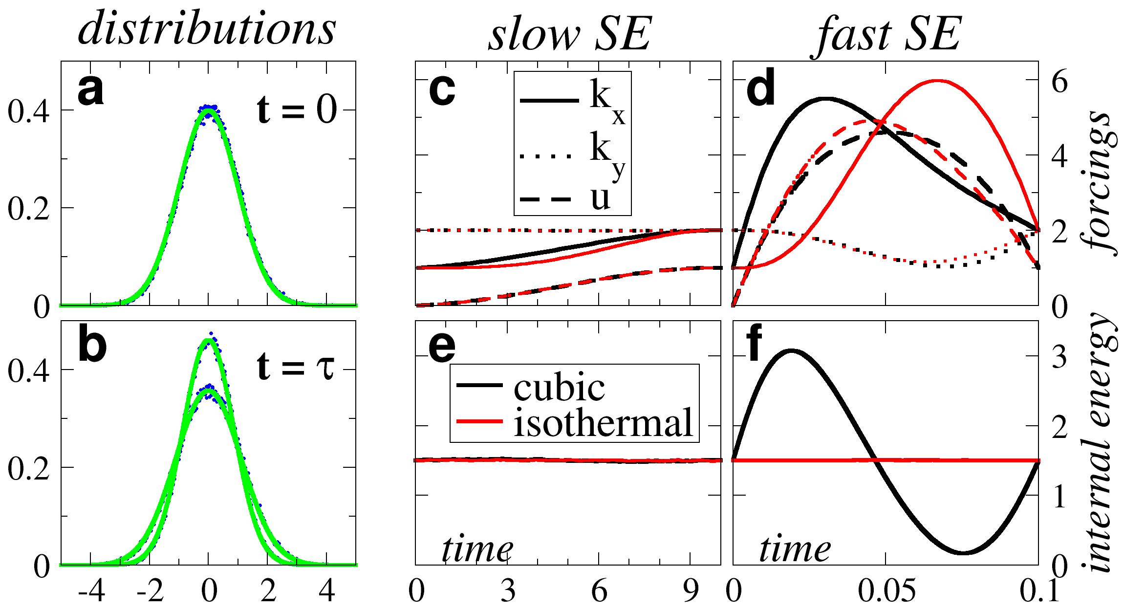
Figure 1: SE in action (details in the Supplementary Information sm ). On the left: a) initial marginal distribution $p(x,t=0)$ and $p(y,t=0)$ (points for simulations) compared with the theoretical stationary distributions (line); b) same quantities at $t=\tau$, the end of the SE transformation. Middle and right plots show the use of two quasi-static protocols, with the same initial and final parameters ${\mathbf{\Pi}}^{i}$ and ${\mathbf{\Pi}}^{f}$: a simple cubic protocol (black) and an isothermal protocol (red). Upper plots: c) forcings for a large $\tau=10$, which are very close to the quasi-static protocol chosen; d) for a much faster SE, $\tau=0.1$, the forcings have large corrections given by Eq. (6). Lower plots e) and f): the values of the internal energy E in the four different cases (cubic and isothermal during slow and fast SE).

Energetics - SE protocols represent an interesting theoretical framework to study energetics and thermodynamics. For instance, we consider internal energy for the model in study:

$$\begin{array}[]{rcl}E&=&\langle V\rangle=\frac{1}{2}k_{x}\langle x^{2}\rangle+\frac{1}{2}k_{y}\langle y^{2}\rangle+u\langle xy\rangle,\end{array}$$

where, calling $\det\Gamma=\gamma_{1}\gamma_{2}-\gamma_{3}^{2}$, we have $\langle x^{2}\rangle=\gamma_{2}/\det\Gamma$, $\langle y^{2}\rangle=\gamma_{1}/\det\Gamma$ and $\langle xy\rangle=-\gamma_{3}/\det\Gamma$. Since during the SE, the distribution parameters $\bm{\gamma}(t)$ depend on the quasi-static protocol as $\bm{\gamma}^{st}[{\mathbfcal{P}}(t/\tau)]$, the expressions for $\langle x^{2}\rangle$, $\langle y^{2}\rangle$ and $\langle xy\rangle$ can be written in terms of the quasi-static protocol (see Supplementary Information sm ). Hence, using the expression for the forcing protocols ${\mathbf{\Pi}}={\mathbfcal{P}}+\frac{1}{\tau}\delta{\mathbfcal{P}}$, one can compute the explicit expression of the internal energy $E$. Remarkably, it turns out, after careful algebra, that this expression is simple:

$$E=\frac{T_{x}+T_{y}}{2}-\frac{1}{\tau}\frac{d}{ds}\left[\frac{\mathcal{K}_{x}T_{y}+\mathcal{K}_{y}T_{x}}{4(\mathcal{K}_{x}\mathcal{K}_{y}-\mathcal{U}^{2})}\right]_{s=t/\tau}.$$ (7)

Several comments about this equation are in order. Firstly we note that during a quasi-static protocol ($\tau\to\infty$) the internal energy is constant, as one could expect: this constant value does not depend on the forcing parameters, neither on $k_{x,y}$ nor on $u$. More interestingly, the finite time correction to the internal energy, can be written with a single differential form $\frac{1}{\tau}\Theta^{\prime}$, where $\Theta=\frac{\mathcal{K}_{x}T_{y}+\mathcal{K}_{y}T_{x}}{4(\mathcal{K}_{x}\mathcal{K}_{y}-\mathcal{U}^{2})}$. An immediate reward of this result is that it allows to identify a specific class of quasi-static protocols, that we call the finite time isothermal protocols, defined as the SE protocols that keep $\Theta$ constant. Using such a quasi-static protocol one can perform a SE procedure with constant internal energy in any finite time $\tau$, provided to force the system with the appropriate finite time corrections (6). In Fig. 1 we show simple numerical simulations giving a demonstration of our results.

Conclusions - Here we have proposed a general framework for studying finite time transformations in stochastic processes under the important request of connecting two steady states without the need of further relaxation time (“swift equilibration”). Our general framework is based upon the idea of fixing an arbitrary quasi-static protocol and then computing the finite-time corrections to it. We have applied our idea to a model (“Brownian gyrator”) with a harmonic potential in contact with two different thermal baths, a minimal non-equilibrium generalization of the celebrated Ornstein-Uhlenbeck process. In this sense, the model can be considered as the harmonic oscillator or the ”perfect gas” for non-equilibrium steady states. Despite the linearity of the model, the problem of SE discloses a rich and promising terrain for theoretical explorations. We give the exact explicit expression for the general SE, and also a simple condition to obtain finite-time transformations that conserve internal energy. The existence of experimental realizations of the steady Brownian gyrator  Ciliberto et al. (2013); Soni et al. (2017); Argun et al. (2017); Chiang et al. (2017) let us foresee interesting experimental investigations of our procedures in the next future. An important theoretical perspective concerns the research of optimal protocols with respect to work or other thermodynamic relevant quantities, for instance a suitable definition of finite-time adiabatic transformations Plata et al. (2020) to the case where two thermal baths are present.