Evolutionary and pulsation properties of Type II Cepheids

We discuss the observed pulsation properties of Type II Cepheids (TIICs) in the Galaxy and in the Magellanic Clouds. We found that period (P) distributions, luminosity amplitudes and population ratios of the three different sub-groups (BL Herculis [BLH, P¡5 days], W Virginis [WV, 5$\leq$P¡20 days], RV Tauri [RVT, P¿20 days]) are quite similar in different stellar systems, suggesting a common evolutionary channel and a mild dependence on both metallicity and environment. We present a homogeneous theoretical framework based on Horizontal Branch (HB) evolutionary models, envisaging that TIICs are mainly old (t$\geq$10 Gyr), low-mass stars. The BLHs are predicted to be post early asymptotic giant branch (PEAGB) stars (double shell burning) on the verge of reaching their AGB track (first crossing of the instability strip), while WVs are a mix of PEAGB and post-AGB stars (hydrogen shell burning) moving from the cool to the hot side (second crossing) of the Hertzsprung-Russell Diagram. Thus suggesting that they are a single group of variable stars. The RVTs are predicted to be a mix of post-AGB stars along their second crossing (short-period tail) and thermally pulsing AGB stars (long-period tail) evolving towards their white dwarf cooling sequence. We also present several sets of synthetic HB models by assuming a bi-modal mass distribution along the HB. Theory suggests, in agreement with observations, that TIIC pulsation properties marginally depend on metallicity. Predicted period distributions and population ratios for BLHs agree quite well with observations, while those for WVs and RVTs are almost a factor of two smaller and larger than observed, respectively. Moreover, the predicted period distributions for WVs peak at periods shorter than observed, while those for RVTs display a long period tail not supported by observations. We investigate several avenues to explain these differences, but more detailed calculations are required to address these discrepancies.

1 Introduction

The coupling between evolutionary and pulsation models has a long-standing tradition. The reason is threefold. Firstly, pulsation models involve the stellar envelope, i.e. the portion of a stellar structure located between the region affected by nuclear burning and the stellar atmosphere. This means that they rely on the mass-luminosity relations and their temporal evolution predicted by evolutionary models.

The comparison between pulsation predictions (periods, amplitudes, modal stability) and observations provide independent constraints on the input parameters (chemical composition) and on the micro- (opacity, equation of state) and the macro- (mass loss, convective transport) physics adopted to construct evolutionary and pulsation models.

Finally, although the classification of variable stars is based on their pulsation properties and the morphology of the light curve, the evolutionary properties of variables stars provide fundamental insights on their progenitors and their different evolutionary channel(s).

Seminal investigations concerning the coupling between evolutionary and pulsations models date back to the seventies, and have provided a firm evolutionary scenario for RR Lyraes (RRLs)(Iben & Huchra 1970; Tuggle & Iben 1973), Classical Cepheids (CCs)(Kippenhahn et al. 1967; Fricke et al. 1971; Becker et al. 1977) and Mira (Vassiliadis & Wood 1993) variables.

The improvement in the input physics (radiative [OP, Iglesias & Rogers (1996); OPAL, Seaton (2007)] and molecular [Ferguson et al. (2005)] opacities) and in the treatment of the convective transport provided a new spin for both radial (Buchler & Goupil 1988; Chiosi et al. 1993; Kovacs & Buchler 1993; Bono & Stellingwerf 1994; Bono et al. 2000) and nonradial (Dziembowski & Cassisi 1999; Guzik et al. 2000) pulsators. The comparison between theory and observations experienced a significant step forward thanks to detailed grids of bolometric corrections and color-temperature transformations covering a broad range of chemical compositions, based on theoretical model atmospheres (Gustafsson et al. 1975; Kurucz 1979; Castelli et al. 1997; Castelli & Kurucz 2003; Gustafsson et al. 2008).

In spite of the crucial role that type II Cepheids (TIICs played in the cosmic distance scale (Baade 1958; Bono et al. 2016) and the ongoing observational effort for the identification in the Galactic center (Matsunaga et al. 2013; Braga et al. 2019), in the Galactic Bulge (Soszyński et al. 2011, 2017), in Galactic clusters (Matsunaga et al. 2006) and in the Magellanic Clouds (Soszyński et al. 2018) the investigations concerning their evolutionary and pulsation properties lag when compared with other groups of radial variables. According to their pulsation properties (period distribution, shape of the light curve) TIICs can be classified into three different sub-groups (Soszyński et al. 2008): BL Herculis (BLH) have periods longer than RRLs (P$\gtrsim$1 day) and shorter than five days, W Virginis (WVs) have periods between five and twenty days, while RV Tauri (RVTs) have periods longer than twenty days (see Fig. 1). Although, the number of TIICs known in the literature increased by more than one order of magnitude in the last decade, detailed investigations concerning their evolutionary properties date back to the late seventies, early eighties. Gingold (1974, 1976, 1985) provided exhaustive evolutionary calculations covering a broad range of stellar masses and chemical compositions. More recently, evolutionary and pulsation properties of TIICs were also investigated by Bono et al. (1997c) and Di Criscienzo et al. (2007), but their analyses were limited to short-period TIICs (BLHs).

The empirical scenario concerning TIICs has been enriched by several new interesting results. Based on detailed multi-band investigation of Magellanic Cloud (MC) TIICs, Groenewegen & Jurkovic (2017a) found that binary star evolution has to be taken into account for explaining their location in the Hertzsprung-Russell diagram (HRD). Note that binarity was originally invoked by Soszyński et al. (2008) to explain the position in the Period-Wesenheit (PW) diagram of a sub-group of TIICs that, at fixed period, were systematically brighter than canonical TIICs. More recently, it has been suggested by Iwanek et al. (2018) that MC TIICs might also have intermediate-age (0.5$\lesssim$t¡10 Gyr) progenitors. Indeed, their 3D spatial distribution does not match that of RRLs (old, t$\geq$10 Gyr, stellar tracers), but it is half-way between RRLs and CCs (young—t$\lesssim$300 Myr—stellar tracers).

Finally, it is worth mentioning that both the evolutionary channel producing RVTs and their pulsation properties are not clear yet. Indeed, observations suggest that this sub-group of TIICs includes both low-mass ($\sim$0.5 $M_{\odot}$), and intermediate-mass ($\sim$1-2 $M_{\odot}$) stars. Moreover, the occurrence of alternating deep and shallow minima in the light curve and of infrared excess caused by circumstellar dust still lack a quantitative explanation. In this context it is worth mentioning that it is not even clear whether RVTs do follow the same Period-Luminosity (PL) relation of TIICs (Matsunaga et al. 2006; Bhardwaj et al. 2017; Wallerstein 2002; Ripepi et al. 2015).

The motivation for this investigation is threefold. Firstly, recent evolutionary grids of advanced evolutionary phases for low-mass stars cover a broad range in heavy elements and helium abundances. The same outcome applies to nonlinear, convective hydrodynamical models (Marconi & Di Criscienzo 2007; Marconi et al. 2015, 2018). Moreover, synthetic HB models are nowadays able to provide firm predictions concerning both evolutionary and pulsation models (Savino et al. 2015).

On the observational side, long term optical (OGLE-IV, Catalina, PTF, PanStarrs, SDSS) and NIR (VVV, VMC, IRSF) surveys are providing a wealth of new identifications together with accurate pulsation properties (mean magnitudes, periods, luminosity amplitudes). Moreover, detailed photometric and spectroscopic investigations are opening a new path concerning the presence of TIICs in spectroscopic binaries, with the advantage to have an independent dynamical estimate of their actual stellar mass (Pilecki et al. 2017).

Finally, current theoretical and empirical evidence indicate that the bulk of TIICs have old progenitors. This means that TIICs are excellent tracers of old stellar populations and thanks to their intrinsic brightness ($\log{L}$/$\log{L_{\odot}}>$2) they can be identified in Local Group and in Local Volume galaxies.

The structure of the paper is as follows. In § 2 we summarize the pulsation properties (periods, amplitudes) of TIICs. In particular, we discuss the different classifications that have been suggested in the literature. Evolutionary properties of TIICs are dealt with in § 3, where we address the role that pulsation and evolution play in explaining observed properties of TIICs. In § 4 we discuss a set of synthetic HB models calculated to investigate the observed period distributions of TIICs, while in § 5 we provide preliminary evolutionary calculations taking into account gravo-nuclear loops and He enhancement. In the last section we summarize our results and outlines possible future avenues for this project. Finally, the Appendix focuses on the metallicity distribution of field and cluster TIICs, and comparisons with the corresponding distribution for old stellar tracers (RRLs).

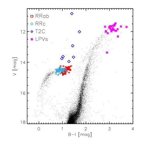
Figure 1: B-I,V Optical Color-Magnitude Diagram of the Galactic globular $\omega$ Centauri (Braga et al. 2016). Black dots display cluster stars, selected according to radial distance and photometric error. The cyan circles and red squares display candidate cluster first overtone (101 RRc, –0.6$\leq\log P\leq$–0.3) and fundamental (85 RRab, –0.33$\leq\log P\leq$0.0) RRLs, respectively (Braga et al. 2016). The blue diamonds denote TIICs (7, 0.05$\leq\log P\leq$1.5)), based on mean magnitudes derived in Braga et al. (2020, in preparation). The magenta asterisks show a selection of cluster Long Period Variables (LPVs, 1.58$\leq\log P\leq$2.72) identified by Lebzelter & Wood (2016), but based on our own photometry.

2 Observed pulsation properties of Type II Cepheids

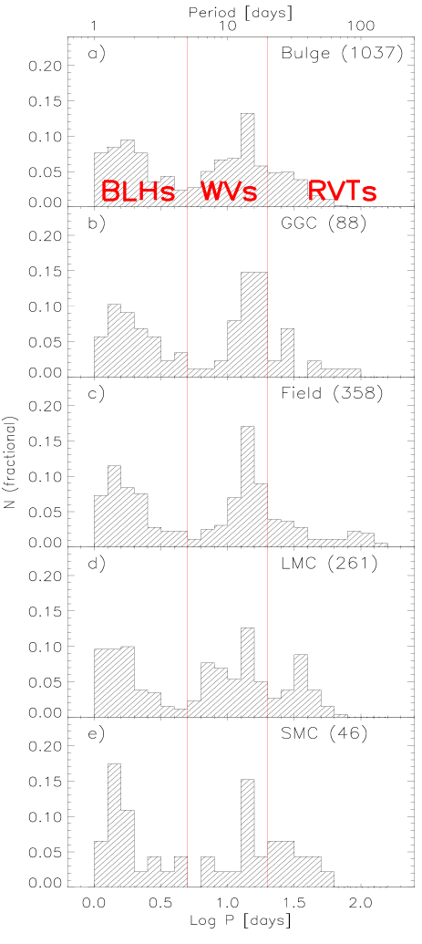
Figure 2: Panel a): Period distribution for TIICs in Galactic Bulge (OGLE-IV, Soszyński et al. 2017). The two red vertical lines display the period boundaries for the three sub-groups: BLHs (P$\leq$5 days), WVs (5$<P\leq$20 days) and RVTs (P$>$20 days) according to Soszyński et al. (2011). The total number of TIICs and the number fractions of the three sub-groups are also labelled. Panel b): Same as Panel a), but for TIICs in Galactic globular clusters according to Clement et al. (2001); Matsunaga et al. (2006); Pritzl et al. (2003). Panel c): Same as Panel a), but for TIICs in the Galactic field according to Ripepi et al. (2019). Panel d): Same as Panel a), but for TIICs in the Large Magellanic Cloud according to Soszyński et al. (2018). Panel e): Same as Panel a), but for TIICs in the Small Magellanic Cloud according to Soszyński et al. (2018).

To constrain the empirical pulsation properties of TIICs we collected data available in the literature for Galactic and MC variables. Concerning the Galactic ones we collected TIICs in the Bulge (OGLE IV, 1037, Soszyński et al. 2017), globular clusters (see Fig. 2) (Clement et al. 2001; Matsunaga et al. 2006; Pritzl et al. 2003) and in the field (Ripepi et al. 2019), while for the Magellanic Clouds ones we employ data provided by Soszyński et al. (2018). Figure 2 shows the period distribution of both Galactic and Magellanic TIICs. They typically range from one to more than one hundred days. Moreover, they display two local minima for P$\sim$5 and P$\sim$20 days. The former one was adopted for separating BLHs from WVs and the current data are, indeed, suggesting that it ranges from about four days in the Bulge to about six days in the Galactic field. The latter one (P$\sim$20 days) was adopted for separating WVs from RVTs, and the current data are suggesting that it shows up as a shoulder in the period distribution of Bulge and field TIICs and as a local minimum in GCs and in MC TIICs.

Data plotted in this figure display several interesting features worth being discussed in more detail.

First of all, the relative fractions of BLHs and WVs are the same within 1$\sigma$ (Poisson uncertainty) when moving from Galactic (panels a, b, c) to Magellanic TIICs (panels d, e). The values are on the order of 40%, suggesting a common evolutionary channel and a mild dependence on the initial metal content. Regarding the fraction of WV in the Small Magellanic Cloud (SMC), the difference is still within 1$\sigma$, but the Poisson uncertainty is twice as large as for the LMC, because the total number of TIICs in this SMC is still limited. An increase by a factor 5-6 in the sample size is required to reach firmer conclusions. The relative fraction of RVTs in the same stellar systems ranges from 15% to 25%. The differences are on the order of 1$\sigma$, but once again, the SMC sample size is limited. Moreover, the period distribution changes significantly when moving from the Bulge to the Galactic field and to the MCs (see Fig. 2). This points to an observational bias due to the possible misclassification of the alternate deep and shallow minima characterizing this group of variable stars (Percy et al. 1991).

Regarding WVs, their period distribution appears to be peaked at $\log P\sim$1.1-1.2, quite uniform in the Bulge and in the LMC, while the distribution is skewed toward longer periods in GCs and in the Galactic field.

Our referee suggested to quantify better the difference in the period distribution of TIICs when moving from the Galaxy to the MCs. We performed a nonparametric, two-tailed Kolmogorov-Smirnov test by assuming the period distribution of the Bulge TIICs as the reference distribution. We found that on average the probability of the null hypothesis –that the two distributions come from the same population– is on the order of $\sim$60% for the pairs Bulge–SMC and Bulge–Halo, while it increases to 73% for the pair Bulge–GGCs, and to 92% for the pair Bulge–LMC. The variation of the probability of the null hypothesis by almost 50% when moving from the pairs Bulge–SMC/Bulge–Halo to the pair Bulge–LMC further supports the broad variety of TIICs in different environments.

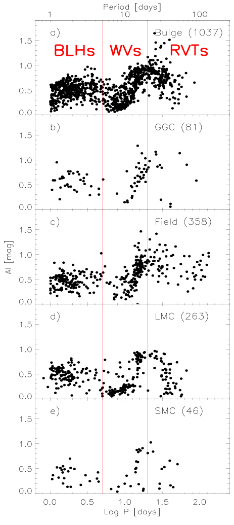
Figure 3: I-band amplitude versus logarithmic period (Bailey diagram) for Bulge TIICs (panel a), GC TIICs (panel, b), Galactic field TIICs (panel c), Large Magellanic Cloud TIICs (panel d) and Small Magellanic Cloud TIICs (panel e). The red vertical lines are the same as in Fig. 2 (see text for more details).

The difference in the period distribution among BLHs, WVs and RVTs is fully supported by the Bailey diagram, the $I$-band luminosity amplitudes versus logarithmic period shown in (Fig. 3). The $I$-band amplitudes for Bulge and Magellanic TIICs were provided by Soszyński et al. (2017, 2018). For GGCs, we adopted the $B$-, $V$- and $K$-band luminosity amplitudes of cluster TIICs from Clement et al. (2001) and transformed them into the $I$-band employing the amplitude ratios derived by Braga et al. (2020, in preparation). The latter ratios were derived using OGLE $VI$- and VVV $K_{s}$-band light curves of Bulge TIICs and $BV$-band light curves of TIICs in GGCs. The Bailey diagram shows that WVs attain a well defined minimum at P$\sim$8 days, with a steady increase toward longer periods. The trend for RVTs is far from being homogeneous, because the maximum around twenty days is broad. Moreover, RVTs in the Bulge and in the LMC display a steady decrease toward longer periods and a well defined cut-off at periods longer than 60 days. On the other hand, RVTs in the Galactic field approach 200 days and display at fixed period a broad range in luminosity amplitudes.

The current partition of TIICs into three sub-groups follows the classification suggested by Soszyński et al. (2008, 2011). They also suggested a new group of TIICs, the peculiar WVs (pWVs) which have peculiar light curves. Moreover the pWVs are, at fixed period, brighter than typical TIICs. These are the reasons why the pWVs are not included in this analysis. Data plotted in Fig. 2 and in Fig. 3, based on observables that are independent of distance and reddening, shows that the current classification is plausible. However, the boundaries of the different sub-groups might be different in different stellar systems, suggesting that the environment and the mean metallicity might globally affect their properties.

The possible dependence on the metallicity requires a more detailed discussion. We still lack spectroscopic measurements of Bulge TIICs, so we assume that their metallicity distribution is either similar to the one of Bulge RRLs as measured by Walker & Terndrup (1991), suggesting a mean [Fe/H]=$-$1.0 with a 0.16 dex standard deviation, or similar to Bulge red giant stars, with average [Fe/H]=$-$1.5 and a standard deviation equal to 0.5 dex (Rich et al. 2012; Zoccali et al. 2017). The metallicity distribution of TIICs in GCs and in the Galactic field ranges from [Fe/H]$\sim-$2.4 to slightly super solar [Fe/H] (see Appendix A). Concerning LMC TIICs, we can follow two different paths. According to Gratton et al. (2004b) the metallicity of LMC RRLs based on low-resolution spectra range from [Fe/H]=–2.1 to [Fe/H]=–0.3, but only a few stars are more metal-rich than [Fe/H]=–1, indeed, the mean metallicity for 98 RRLs is [Fe/H]=–1.48$\pm 0.03\pm 0.06$. This metallicity range is also supported by recent investigations concerning the mean metallicity of LMC globular clusters. Using homogeneous Stroemgren photometry, Piatti & Koch (2018) found, in agreement with spectroscopic measurements, that the metallicity of the ten LMC globulars ranges from $-$2.1 dex (NGC 1841) to $-$1.1 dex (ESO121-SC3). We still lack direct measurements of the metallicity distribution of truly old SMC stellar tracers, however the metallicity of NGC 121, the only SMC globular cluster, is [Fe/H]=$-$1.28, according to high resolution spectroscopy (Dalessandro et al. 2016). Table 4 gives either the mean metallicity or the metallicity range of the stellar systems included in Fig. 10. The above evidence shows that the TIICs plotted in Fig. 10 cover roughly three dex in metal abundance, but the population ratios appear to be, within the errors, quite similar.

Table 1: Population ratios for TIICs in different Galactic components and in the Magellanic Clouds.

Type	Environment
	Halo	Bulge	GGC	LMC	SMC
BLH	0.408$\pm$0.040	0.431$\pm$0.024	0.432$\pm$0.084	0.379$\pm$0.045	0.435$\pm$0.116
WV	0.439$\pm$0.042	0.405$\pm$0.023	0.420$\pm$0.082	0.410$\pm$0.047	0.326$\pm$0.097
RVT	0.154$\pm$0.022	0.164$\pm$0.014	0.148$\pm$0.044	0.211$\pm$0.031	0.239$\pm$0.080

3 Properties of Type II Cepheids

TIICs have been the cross-road of several theoretical and empirical investigations, however, their evolutionary status is far from being well established. A first analysis of the evolutionary properties of TIICs was provided over 40 years ago by Gingold (1974, 1976, 1985). He recognized that a significant fraction of hot (blue) HB stars evolve off the Zero-Age-Horizontal-Branch (ZAHB) from the blue (hot) to the red (cool) region of the CMD. In the approach to their AGB track these stars are in a double shell (hydrogen and helium) burning phase (Salaris & Cassisi 2005) and cross the instability strip at luminosities systematically brighter than typical RRLs. The difference in luminosity and the smaller mass compared to RRLs induce an increase in the pulsation period of TIICs when compared with RRLs. Typically, the two classes are separated by a period threshold at one day. This separation is supported by a well defined minimum of the period distribution when moving from RRLs to TIICs, but the physical mechanism(s) causing this minimum are not yet clear, and the exact transition between RRLs and TIICs has not been established yet (Braga et al. in preparation).

The quoted calculations suggested also that blue HB stars after the first crossing of the instability strip experience a co-called ‘blue nose’ (then dubbed ‘Gingold’s nose’), e.g. a blue-loop in the CMD, that causes two further crossings of the instability strip before the tracks reach the AGB. These three consecutive excursions were associated to the interplay between the helium and hydrogen burning shells. After core helium exhaustion, HB models with massive enough envelopes evolve redwards in the CMD. The subsequent shell helium ignition causes a further expansion of the envelope, and in turn, a decrease in the efficiency of the shell hydrogen burning, which causes a temporary contraction of the envelope, and a blueward evolution in the CMD. Once shell hydrogen burning increases again its energy production, these models move back towards the AGB track. Finally, these models would eventually experience a fourth blueward crossing of the instability strip before approaching their white dwarf (WD) cooling sequence (see Fig. 1 in Gingold (1985) and Fig. 2 in Maas et al. (2007)). During their final crossing of the instability strip, models (in the post-AGB phase), are only supported by a vanishing shell H-burning.

Basic arguments based on their evolutionary status and the use of the pulsation relation available at that time (van Albada & Baker 1973) allowed Gingold to associate the first three crossings (including the ‘Gingold’s nose’) to BLHs and the fourth one to the WVs variables.

These early analyses, however, lacked qualitative estimates of the time spent inside the instability strip during the different crossings, and in particular, the period distributions associated to the different crossings. Moreover and even more importantly, dating back to more than 25 years ago, HB evolutionary models based on updated physics inputs, (Lee et al. 1990; Castellani et al. 1991; Dorman & Rood 1993; Brown et al. 2000; Pietrinferni et al. 2006a; Dotter 2008; VandenBerg et al. 2013) do not show the ‘Gingold’s nose’.

3.1 Pulsation properties of Type II Cepheids

We have already discussed in sections 1 and 2 the change in the topology of the instability strip, i.e. the regions in the HRD with stable modes of pulsations for RRLs and TIICs. We adopted the theoretical instability strip for RRLs recently provided by Marconi et al. (2015). Note that the blue and red boundaries have been extrapolated to higher luminosities to cover the luminosity range typical of TIICs. The reason why we decided to follow this approach is twofold. First of all, the instability strips provided by Marconi et al. (2015) cover a broad range in metal abundances, stellar masses and luminosities typical of RRLs. This means that they cover the entire range of RRLs and the short-period range for TIICs. Secondly, this is an exploratory investigation, to trace the global evolutionary and pulsation properties of TIICs. More detailed calculations concerning the topology of the instability strip covering both short- and long-period range of TIICs will be provided in a forthcoming investigation.

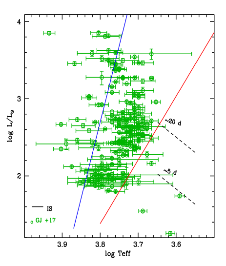
Figure 4: Hertzsprung Russell Diagram (HRD) comparing the predicted (blue and red solid lines) edges of the instability strip and observations for Magellanic TIICs by Groenewegen & Jurkovic (2017a, b). The horizontal error bars display the uncertainty in effective temperature. The black dashed lines display two iso-periodic lines for five and twenty days, respectively.

To validate the predicted boundaries of the instability strip, Fig. 4 shows the comparison in the HR diagram with observations for Magellanic TIICs recently provided by Groenewegen & Jurkovic (2017a, b). Owing to the lack of spectroscopic estimates of the metal abundances, we assumed a metallicity range between $\sim-$2.2 dex and $-$0.7 dex (see Appendix A). To compare theory and observations we derive mean boundaries of the instability strip by taking into account models with metal mass fractions ranging from Z=0.0001 to Z=0.01. Data plotted in this figure shows that theory and observations agree quite well, even though, the predicted instability strips have been computed with a step in effective temperature of 100 K and they have been extrapolated to brighter luminosities.

Moreover, observations display a large spread in effective temperature when moving from fainter to brighter TIICs, but the number of objects hotter than the blue edge is, within the errors, limited. Note that the current predictions for the blue edge of the instability strip are quite solid, since it is minimally affected by uncertainties in the treatment of the convective transport (Baker & Gough 1979). It would be interesting to extend the comparison between theory and observations into optical and near-infrared color magnitude diagrams, to further constrain the plausibility of the current predictions. It is worth mentioning that the predicted strip has a width in temperature ranging from $\approx$1200 K in the period range of BLHs, to $\approx$1600 K in the period range typical of WVs. These estimates agree quite well with similar estimates for the width in temperature of the RRL instability strip (Bono & Stellingwerf 1994; Tammann et al. 2003). A wider instability strip for TIICs would cause a dispersion in luminosity at fixed period, significantly larger than currently observed.

The anonymous referee suggested a more quantitative assessment of the width in temperature of the instability strip. We selected RRLs, TIICs and CCs in the LMC, because they are complete samples (OGLEIV, Udalski et al. 2015) and used the standard deviation of the PW($I$,$V-I$) relation as a proxy for the width in temperature of the instability strip (Bono et al. 1999, 2008; Madore et al. 2017; Riess et al. 2019). Note that we are using PW relations, because they are independent of uncertainties affecting reddening corrections and also because they mimic a Period-Luminosity-Color relation (Madore 1982; Bono & Marconi 1999). We applied a 3$\sigma$ clipping to remove outliers and we found that the standard deviations range from 0.08 mag for CCs to 0.10 mag for TIICs and to 0.13 mag for RRLs. This result suggests a similar width in temperature of the instability strip when moving from RRLs to CCs.

We also note that the distribution of TIICs inside the instability strip is far from being homogeneous. Indeed, the current observations display two well defined clumps: a fainter one located at $\log L/L_{\odot}\approx$2.0 and $\log T_{eff}\approx$3.80 and a brighter one located at $\log L/L_{\odot}\approx$2.6-2.8 and $\log T_{eff}\approx$3.74. The iso-periodic lines (black dashed lines) indicate that the former group is mainly associated with BLHs variables, given that their periods range from 1 to 5 days, while the latter one is associated to WVs variables with periods roughly ranging from 5 to 20 days. The predicted periods were estimated using the fundamental pulsation relation provided by Marconi et al. (2015). This relation depends on stellar luminosity, effective temperature, stellar mass and chemical composition. For the first two parameters we are using individual values (HRD), while for the last two we are using plausible mean values. The correlation with the period distributions plotted in Fig. 2 is quite obvious.

3.2 Evolutionary properties of HB models

The evolutionary properties of low-mass core helium burning models have been discussed in several recent investigations (Cassisi & Salaris 2011, and references therein). Here we summarize the main features relevant to explain the evolutionary channels producing TIICs.

The grey area displayed in the top panel of Fig. 5 outlines the region between the ZAHB (faint envelope) and central helium exhaustion (bright envelope) for a set of HB models with different masses and fixed chemical composition, Z=0.01 and He mass fraction Y=0.259. We have assumed an $\alpha$-enhanced chemical composition (Pietrinferni et al. 2006b) and a progenitor mass according to a 13 Gyr isochrone (the mass at the main sequence turn off –MSTO– is equal to 0.86 $M_{\odot}$).

As well known, along the ZAHB the total mass of the models decreases when moving from the red HB (RHB) to the blue HB (BHB) and further on to the Extreme HB (EHB). The helium core mass is constant along the ZAHB and it is mainly fixed by the chemical composition of the progenitor ($M_{c}^{He}$=0.4782 $M_{\odot}$) and is roughly independent of age for ages above a few Gyr. The mass of the envelope decreases from 0.4218$M_{\odot}$ for RHB models to a few thousandths of solar masses for EHB models. In an actual old stellar population with a fixed initial chemical composition, the mass lost along the RGB (more efficient when approaching the tip of the RGB, Origlia et al. 2014) determines the final mass distribution along the ZAHB.

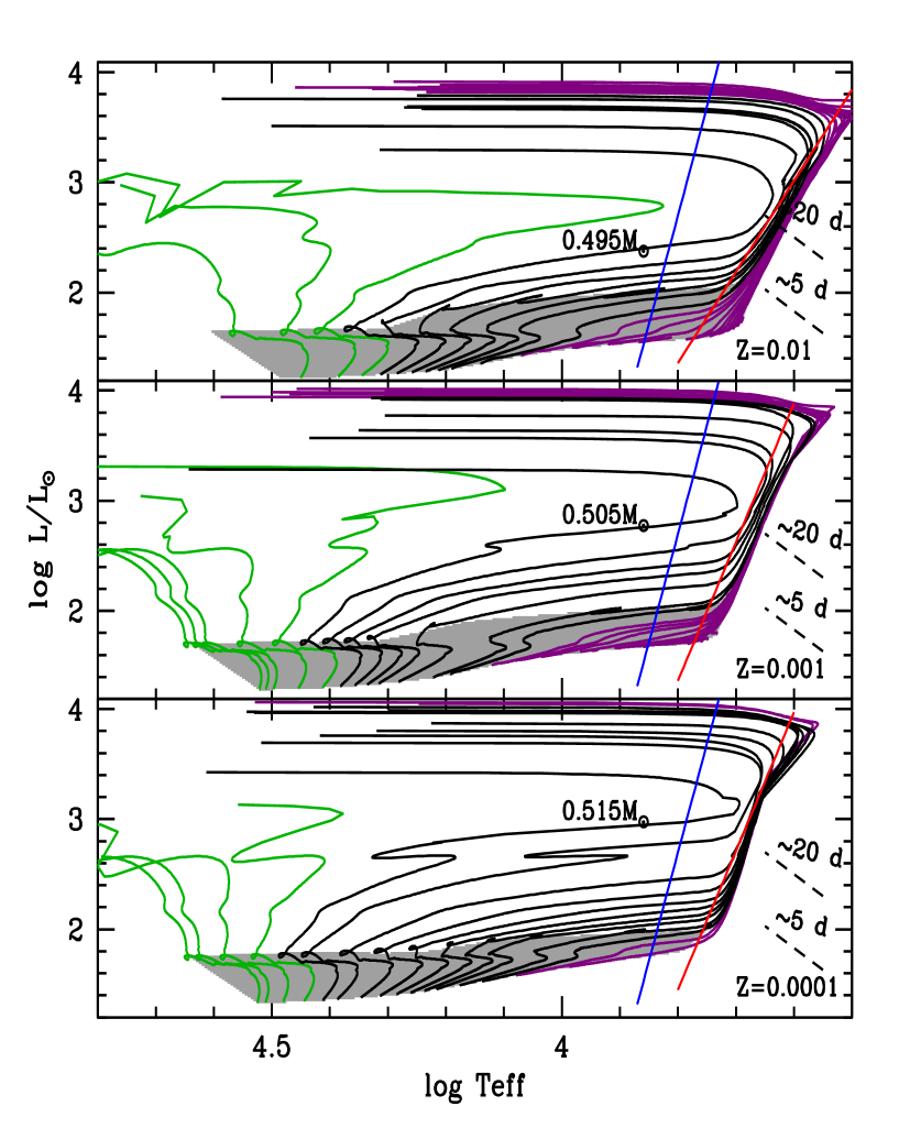
Figure 5: Top: HRD of HB evolutionary models covering a broad range of stellar masses (M/M_⊙=0.48–0.90) and the same initial chemical composition (Z=0.01, Y=0.259). The grey area outlines the region between ZAHB (faint envelope) and central helium exhaustion (bright envelope). The green lines display HB models evolving as AGB-manqué, black lines the post early-AGB models and purple lines the thermal pulsing AGB ones (see text for more details). The almost vertical blue and red solid lines mark the hot and cool edges of the Cepheid instability strip. The minimum stellar mass (solar units) crossing the instability strip is labelled in black. The black dashed lines display two iso-periodic lines for 5 and 20 days. Middle: Same as the top panel, but for stellar masses ranging from M/M_⊙=0.4912 to 0.80 and for a metal-intermediate chemical composition (Z=0.001, Y=0.246). Bottom: Same as the top panel, but for stellar masses ranging from M/M_⊙=0.5035 to 0.70 and for a metal-poor chemical composition (Z=0.0001, Y=0.245).

The bright envelope of the grey area marks the central helium exhaustion, corresponding formally to the beginning of the AGB phase. The small ripples along the helium exhaustion sequence ($\log L/L_{\odot}\sim$1.8) display that the lower the total mass of the HB model, the hotter the effective temperature at which the helium exhaustion takes place. The luminosity of the ripples ranges from $\log L/L_{\odot}\approx$2 in the warm region to $\log L/L_{\odot}\approx$1.6 in the hot region of the HB. At this point the He-burning moves smoothly to a shell around the carbon-oxygen core. The overlying H-shell extinguishes, due to the expansion of the structure before reigniting later with various efficiencies, depending on the mass thickness of the envelope around the original He core.

Models with mass below 0.495$M_{\odot}$ (corresponding to an envelope mass lower than about 0.017$M_{\odot}$) never reach the AGB location, they do not cross the instability strip and move to their WD cooling sequence, as a carbon-oxygen (CO) WD (Castellani et al. 2006; Bono et al. 2013; Salaris et al. 2013). These objects have been called AGB-Manqué (Greggio & Renzini 1990), and are shown as green tracks in the top panel of Fig. 5).

More massive models do cross the instability strip while moving towards their AGB tracks. Models with $0.495\leq M/M_{\odot}<0.55$ do reach the AGB but move back towards the WD sequence (hence they cross the instability strip again but at higher luminosities) well before reaching the thermal pulse (TP) phase. They are named post early-AGB (PEAGB), and are plotted as black lines in the top panel of Fig. 5. These AGB models perform several gravo-nuclear loops in the HRD, either during the AGB phase and/or in their approach to the WD cooling sequence after leaving the AGB (during this post-AGB transition models cross again the instability strip). Some of them may take place inside the instability strip. The reader interested in a more detailed discussion concerning their impact on the pulsation properties is referred to Bono et al. (1997a, b). The evolutionary implications, and in particular the impact of the loops concerning the AGB lifetime have been recently discussed by Constantino et al. (2016).

Models with $M\geq 0.54M_{\odot}$ (plotted as purple lines in Fig. 5) do evolve along the AGB and experience the TPs. The number of TPs, and in turn, the duration of their AGB phase is once again dictated by the efficiency of the mass loss, and by their residual envelope mass (Weiss & Ferguson 2009; Cristallo et al. 2009). Calculations of TP evolution are quite demanding from the computational point of view, hence we decided to use the fast and simplified synthetic AGB technique originally developed by Iben & Truran (1978) and more recently by Wagenhuber & Groenewegen (1998), to compute the approach of these AGB models to the WD cooling sequence. In particular, the synthetic AGB modelling started for thermal-pulsing-AGB (TPAGB) models just before the occurrence of the first TP, while for PEAGBs it was initiated at the brightest and reddest point along the first crossing of the HRD, towards the AGB.

The middle and the bottom panels of Fig. 5 show the same predictions, but for two more metal-poor chemical compositions. The values of the stellar masses plotted along the ZAHBs show the impact of the chemical composition. The mass range of the tracks which cross the instability strip and produce TIICs steadily decrease from 0.495–0.90 $M/M_{\odot}$ for Z=0.01, to 0.505–0.80 $M/M_{\odot}$ for Z=0.001 and to 0.515–0.70 $M/M_{\odot}$ for Z=0.0001. It is worth mentioning that the range in luminosity covered by the different sets of models is relatively similar. The mild change in stellar mass and the similarity in luminosities suggests a marginal dependence of the mass-luminosity (ML) relation of TIICs on the chemical composition.

3.3 Pulsation and evolutionary implications for Type II Cepheids

The marginal dependence of the ML relation for TIICs on chemical composition does not imply similar period distributions in different stellar systems. To investigate in more detail this issue we plotted in Fig. 5 the instability strips predicted by Marconi et al. (2015) for the various metal abundances. Data plotted in this figure show that the instability strip covers a broader range in effective temperatures when moving from metal-poor to metal-rich models. Moreover, HB evolutionary models become, as expected, systematically redder when increasing the initial metallicity. These two circumstantial evidence indicates that both the period distribution and the evolutionary time spent inside the instability strip do depend on the metal content.

A glance at the predictions plotted in this figure show that PEAGB models during either the first and partially during the second crossing of the instability strip can explain the typical period range of both BLHs and WVs. The increase of the pulsation period when moving from BLHs to WVs stems from the increase in luminosity and the decrease in stellar mass (see Fig. 5). The evolutionary times spent inside the instability strip for the two crossings and for selected stellar masses are listed in Table 3. Note that the stellar masses, at fixed chemical composition, were selected to be representative of the stellar structures crossing the instability strip.

Table 2: Predicted population ratios based on synthetic AGB models by assuming an uncertainty of $\pm$50 K on the boundaries of the instability strip (see text for details).

Z	Ntot	NBLH/Ntot	NWV/Ntot	NRVT/Ntot
—Uniform mass distribution—
0.0001	262$\pm$43	0.46$\pm$0.03	0.15$\pm$0.03	0.39$\pm$0.01
0.001	185$\pm$22	0.57$\pm$0.06	0.12$\pm$0.01	0.31$\pm$0.02
0.01	160$\pm$21	0.51$\pm$0.02	0.19$\pm$0.03	0.30$\pm$0.01
—Bi-modal mass distribution—
0.0001	115$\pm$7	0.42$\pm$0.05	0.27$\pm$0.05	0.31$\pm$0.02
0.001	98$\pm$7	0.41$\pm$0.03	0.20$\pm$0.02	0.39$\pm$0.02
0.01	105$\pm$28	0.43$\pm$0.04	0.23$\pm$0.05	0.34$\pm$0.01

To further define the theoretical framework for RVTs stars (Wallerstein 2002; Soszyński et al. 2011), we suggest that they are the progeny of both PEAGB and TPAGB. Reasons supporting this hypothesis are the following:

a) Period range – The theoretical periods for these models are systematically longer than WVs and more typical of RVTs stars. The predicted mass for these structures is uncertain, because it depends on the efficiency of mass loss during the TP phase. The theoretical framework is further complicated by the fact that the number of TPs also depends on the initial mass of the progenitor and on its initial chemical composition. This means that it cannot be a priori excluded a contribution from intermediate-mass stars. However, the lack of RVTs in nearby dwarf spheroidal galaxies hosting a sizable fraction of intermediate-mass stars with ages ranging from 1 Gyr to more than 6-8 Gyrs such as (Carina, Fornax, Sextans; Aparicio & Gallart (2004); Beaton et al. (2018)) is suggesting that this channel might not be very efficient. However, RVTs have been identified in the MCs (Soszyński et al. 2008; Ripepi et al. 2015).

b) Alternating cycle behaviour – There is evidence of an interaction between the central star and the circumstellar envelope possibly causing the alternating cycle behaviour (Feast et al. 2008; Rabidoux et al. 2010). The final crossing of the instability strip before approaching the WD cooling sequence either for PEAGB or for TPAGB models appears a very plausible explanation.

The above circumstantial evidence suggests that the variable stars currently classified as TIICs have a range of evolutionary properties. The BLHs and the WVs appear to be either post-ZAHB (AGB, double shell burning) or post-AGB (shell hydrogen burning) stars, while RVTs are mainly post-AGB objects.

Pulsation and evolutionary results plotted in Fig. 5 display a few interesting features worth being discussed.

We start with the ML relation, noticing that current models show that the mass of TIICs during the first crossing is steadily decreasing when we move from fainter to brighter structures. The opposite happens during the second crossing, i.e. the brighter the stellar structure, the larger the stellar mass. However, the difference in stellar mass along first and second crossing is smaller than 10%. This is the reason why the pulsation period is steadily increasing over the entire luminosity range. This increase is driven by the increase in luminosity (see the luminosity coefficients in the fundamental pulsation relation provided by Marconi et al. 2015).

It is worth mentioning that the ML relation for TIICs is significantly different than for both CCs and RRLs. An increase in mass causes, for the former variables, an increase in the mean luminosity, and in turn, in the pulsation period. In the latter group the difference in mass is quite modest inside the instability strip, and the increase in pulsation period is mainly driven by a decrease in effective temperature.

A second point to discuss concerns the pulsational period changes. The evolutionary framework we are outlining has some relevant consequences concerning the period changes of the variables. The BLHs should mainly display positive period changes, due to their main redward evolution. The only exceptions are in the short period regime since they evolve along their blueward excursion, and therefore they might experience both negative and positive period changes. The same behaviour is also expected for WV variables due to their main redward and partial blueward evolution. The main difference being that the redward evolution is systematically slower than the blueward one. Indeed, the duration of the first crossings of the instability strip are on average on the order of a few Myrs, while the second crossings are from a few times to one order of magnitude faster, depending on the stellar mass (Salaris et al. 2008; Bono et al. 2013). Therefore, the positive period changes should be on average more typical than the negative ones. Moreover, the negative period changes should mainly affect the long-period tail of WVs. These qualitative explanations rely on the assumption that these models do not experience gravo-nuclear loops inside the instability strip, which could significantly affect the previous inferences (Bono et al. 1997a, b), with period changes showing alternating positive and negative values.

Finally, the RVTs should be mainly dominated by negative period changes, as a consequence of their blueward evolution. This is true only in case their evolution is not affected by the TP phase. In this case they might experience both positive and negative period changes.

4 Synthetic HB models

In the theoretical framework outlined in Section 3, the post-early AGB stars produce BLHs and short period WVs when they are in the double shell evolution and longer period WVs just before they approach their WD cooling sequence. Finally, TPAGBs evolving towards their WD cooling sequence produce long-period RVTs. For a more quantitative analysis we have computed three sets of synthetic models to account for the evolutionary times spent inside the predicted instability strips. The synthetic HB models have been computed with the code fully described in Dalessandro et al. (2013), and adapted to the problem at hand.

We decided to follow a simple approach: For each of the three initial chemical compositions of Fig. 5, we computed synthetic HB models employing the same tracks as in the figure, assuming at first an uniform mass distribution from the extreme HB to the red HB (the values of $Y$, $Z$ and mass ranges are given in the figure caption). In brief, the synthetic HBs were calculated as follows.

For a given $(Z,Y)$ pair (the He abundance is kept constant at fixed $Z$) we first select randomly (uniform probability) a value of the HB mass $m_{s}$ in the appropriate mass range, and the corresponding HB track is determined by interpolation in mass among the available set of HB tracks at that metallicity.

As a second step, the position of this HB mass $m_{s}$ in the HRD is determined according to its location along the track after a HB evolutionary time $t_{ev}$ has been randomly extracted. With the standard assumption that stars are fed to the ZAHB at a constant rate, $t_{ev}$ is calculated by selecting randomly (uniform probability) an age ranging from zero to $t_{tot}$, where $t_{tot}$ denotes the time spent from the ZAHB to the end of the computed evolutionary sequence with the longest lifetime. This implies that for some value of $m_{s}$ the randomly selected $t_{ev}$ will be longer than the lifetime covered by the corresponding track or, in other words, that this mass has already evolved beyond the last evolutionary point covered by the calculations. Finally, to properly sample fast evolutionary phases, we included in our simulations a large number of synthetic stars (N=50,000). As we have tested by altering the value of N, this number is high enough to ensure that the derived number ratios of the variables are statistically robust.

For each simulation Fig. 6 shows the HRD of the synthetic stars. The stellar structures located inside the instability strip and producing TIICs were marked with asterisks.

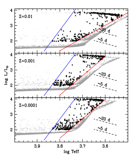
Figure 6: Same as Fig. 5, but for synthetic HB models. Objects inside the instability strip and producing TIICs are marked with asterisks. Those either falling outside the instability strip or producing RRLs are marked with grey dots.

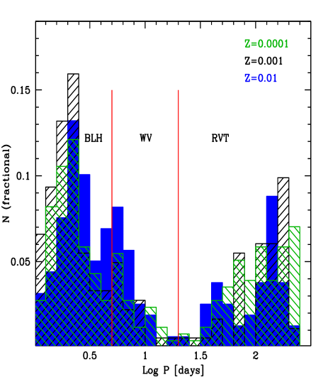
Figure 7: Predicted period distributions for TIICs with different chemical compositions (the colour coding is labeled). Results are based on synthetic HB models (see Fig. 5) calculated by assuming an uniform mass distribution along the HB. The two vertical red lines display the boundaries at 5 and 20 days, respectively. The different subgroups of TIICs are also labelled.

4.1 Predicted period distributions

Figure 7 shows the predicted period distributions, based on the fundamental pulsation relation by Marconi et al. (2015), for the three adopted chemical compositions. The TIIC pulsation properties marginally depend on the metal content, in fair agreement with observations. Metal-rich (blue hatched area) models show a more pronounced peak at the transition between BLHs and WVs compared to observations, while metal-intermediate (black hatched area) and metal-poor (green hatched area) models display a small difference in the short-period tail ($\log P\sim$0.15) for the BLHs and in the long-period tail for RVs ($\log P\sim$2.3). However, predictions based on an uniform mass distribution shows two discrepancies with observations. i) The period distributions for RVTs attain their maxima at periods longer than 100 days, while data plotted in Figures 2 and 3 display only a few objects in this range. ii) The empirical periods in the WV regime display a well defined peak at values ranging from 12 to 16 days. On the other hand, the corresponding theoretical predictions display a peak at periods around six days and a steady decrease in approaching the transition between WVs and RVTs.

Table 3: Evolutionary times spent inside the instability strip for different HB models constructed assuming, respectively, synthetic AGB modelling, full evolutionary calculations (Gravo–nuclear loops), and He-enhanced (Y=0.30) chemical composition.

Z	Stellar Mass	Synthetic HB	Gravo–nuclear loops	He-enriched
	[M⊙]	[Myr]	[Myr]	[Myr]
0.0001	0.525	1.28	0.51	3.19
0.001	0.525	1.10	0.28	2.59
0.01	0.505	4.05	3.2	5.66

To quantify the dependence of the various types of variables on the chemical composition, we estimated the population ratios, i.e. the number of BLHs, WVs and RVTs over the total number of TIICs. Values listed in Table 2 show that the population ratios show marginal variations, when moving from the metal-rich to the more metal-poor regime. However, the population ratios for BLHs are 20% larger than observed, while those for WVs and RVTs are almost three times smaller and two times larger than observed, respectively (see Fig. 2). Note that the standard deviations associated to the population ratios listed in Table 2 take into account uncertainties (by $\pm$50 K) on the effective temperature of the predicted boundaries of the instability strip.

4.2 Bimodal mass distribution along the HB

Theory and observations (Castellani et al. 2003) suggest that the mass distribution along the HB is far from being uniform. Moreover, GCs showing extended HBs also display well-defined gaps in the HB luminosity function (Castellani et al. 2007; Torelli et al. 2019). To investigate the impact of a non-uniform mass distribution on the predicted periods, we computed synthetic HB models for a metal-poor chemical composition (Z=0.0001) and a bimodal Gaussian mass distribution centred on two different mean stellar masses (M=0.535, 0.57 $M_{\odot}$), with the same standard deviation ($\sigma$=0.005 $M_{\odot}$). These simulations are calculated in exactly the same way as for the case of a uniform mass distribution. The only difference is that in the first step of the calculations, the masses $m_{s}$ of the synthetic stars are now randomly selected according to Gaussian distributions with prescribed mean values and $\sigma$ dispersions.

We performed a number of numerical experiments by changing the two mean values to obtain population ratios and period distributions of variables similar to the observed ones. The period distribution based on metal-poor synthetic HB models is plotted as a green hatched histogram in Fig. 8. The new period distribution globally agrees with observations, indeed, it naturally shows a double peak. The peak in the BLH regime agrees quite well with observations, and the whole period distribution covers a similar range in periods. The gap between BLH and WVs appears to be located around four–five days, instead of five days. The main difference is in the WV regime, where the predicted peak in the period distribution is located around six days instead of 12-16 days. The increase either by a factor of ten (black hatched histogram in Fig. 8) or by a factor one hundred (blue hatched histogram in Fig. 8) in metal content has a marginal impact on the position of the peak in the period distribution of WVs. Notice that the metal-intermediate and metal-rich synthetic HB models, to match observational constraints coming from different stellar populations, have been calculated with different choices of the mean stellar masses (see labeled values), but the same standard deviation ($\sigma$=0.005 $M_{\odot}$). The discrepancy concerning the predicted period distribution for RVTs appears to be partially mitigated, because they move towards shorter periods. However, predicted periods for RVTs are systematically longer than observed.

Interestingly, the population ratios listed in Table 2 show that bimodal mass distributions along the HB take account for the observed ratio for BLHs. The predicted population ratios for WVs and RVTs are still smaller and larger than observed, respectively, but the difference between theory and observations is within a factor of two.

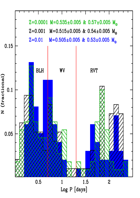
Figure 8: Same as Fig. 7, but for synthetic HB models which assume a bimodal HB mass distribution and the values of the adopted mean masses are labeled. The standard deviations for the mass distributions is the same and equal to 0.005 M_⊙. The two vertical blue lines display the boundaries at five and twenty days, respectively.

5 Detailed evolutionary calculations for off-ZAHB evolution

A detailed comparison between theory and observations would require more detailed synthetic modelling that accounts for a broad range of chemical compositions, progenitor masses and actual HB mass distributions. However, this approach is beyond the aim of the current investigation. We are interested here in providing a global theoretical framework for TIICs, and in particular, to trace the impact that different parameters play in their evolutionary and pulsation properties.

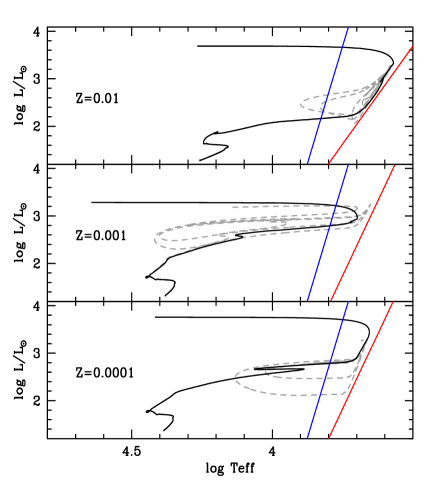
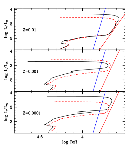
Figure 9: Left: HRD of HB models crossing the instability strip, calculated by assuming an analytical extension for the AGB evolutionary phases (black solid lines) and HB models with the same stellar mass with a full evolutionary computation (dashed black line). From top to bottom the theoretical predictions refer to metal-rich (M=0.505M_⊙), metal-intermediate (M=0.505M_⊙) and metal-poor (M=0.520M_⊙) models. The almost vertical blue and red lines display the edges of the instability strip. Right: Same as the left panel, but the comparison is between standard He (black solid line) and He-enhanced (Y=0.30) models (dashed red lines). See text for details.

As a preliminary step in this direction we have computed in detail the off-ZAHB evolution of some PEAGB models. The left panel of Fig. 9 shows the difference in the off-ZAHB evolution between HB models constructed by assuming the analytical AGB evolution (solid black line) and HB models with the same stellar mass (dashed black line) computed with full evolutionary calculations. The latter one performs, as expected, a series of gravo-nuclear loops inside the instability strip (Bono et al. 1997c). The number can range from a few up to several tens, and depends on the value of the stellar mass and on the chemical composition. Notice that the fully evolutionary models were integrated in time until the mass of the envelope surrounding the He core was smaller than 0.01 M_⊙.

The change in the evolutionary path has a twofold impact on the predicted period distribution. a) The loops took place in a luminosity regime ($\log L$/$L_{\odot}$=2.4-3.0) typical of WVs. This means that they mainly affect the shape and position of the peak in the period distribution located around 10-16 days. b) The evolutionary time spent in this luminosity regime is, on average, several Myrs longer than the evolutionary time based on analytical extensions of AGB evolution (see Figures 6 and 7 in Bono et al. 1997c and Figures 7-10 in Constantino et al. 2016). Note that a significant portion of the red tips of the loops both for the metal-poor and the metal-intermediate chemical composition fall inside the instability strip.

The quoted evidence indicates that direct calculations of low-mass AGB stars appear very promising to constrain the period distribution of WVs. Note that gravo-nuclear loops do not affect evolutionary properties of BLHs. The current evolutionary prescriptions indicate that they are not produced by HB stellar structures with more massive envelopes.

5.1 Dependence of period distribution on primordial helium content

Finally, we have also investigated the dependence of the TIIC period distribution on the initial He content. The right panel of Fig. 9 shows the same HB models (black solid lines, AGB analytical extension) plotted in the left panel, but compared with Y=0.30, He enhanced tracks (and analytical extension of AGB evolution, dashed red line). The enhancement of helium causes an increase of the time spent inside the instability strip ranging from 30% for the metal-rich models, to more than a factor of two for more metal-poor models (see values listed in Table 3). However, synthetic HB models are required to quantify the impact of the helium content on the period distributions. Note that detailed calculations for RRLs in $\omega$ Cen show that an increase in helium mainly causes a systematic shift of the period distribution toward longer periods (Marconi et al. 2015).

6 Summary and final remarks

We have reviewed the evolution and the pulsation properties of TIICs, and propose a new evolutionary characterization of these pulsators. They are mainly old, low-mass stars either during the AGB (double shell burning) or post-AGB (hydrogen shell burning) evolutionary phases. In particular, BLHs are envisaged to be mainly PEAGB stars that are still approaching their AGB track, while WVs are a mix of PEAGB and post-AGB stars along their second crossing of the instability strip (moving from the cool to the hot side of the HRD). This indicates that BLHs and WVs share the same evolutionary channel, therefore, they should be considered a single group of variable stars. The RVTs are predicted to be a mix between post-AGB stars along their second crossing (short-period tail) and TPAGB stars (long-period tail) moving towards the WD cooling sequence. From the evolutionary point of view, TIICs are much more complex than RRLs and CCs, which are in their core He burning plus shell H burning phase. Moreover, it is not clear yet the role that binarity plays in shaping their properties.

Moreover, the current theoretical framework suggests that blue (low-mass) HB stars in their first crossing of the instability strip produce both BLHs and WVs. This means that these variables are not associated with TPAGB stars crossing the instability strip during the so-called ‘blue nose’ (or ‘Gingold’s nose’). Moreover, it soundly supports the very first dynamical mass measured by Pilecki et al. (2018) by using a double-lined binary system including a TIICs (M=0.64$\pm$0.02 M_⊙).

Futhermore, we addressed the following key points.

$\#$ Periods– The observed period distributions of TIICs in different stellar systems (Galactic bulge, Galactic globular clusters, Magellanic Clouds) display a broad similarity. There are small differences concerning the positions of the gaps in the distributions, but it is not clear whether they are a consequence of the environment (cluster versus field) or possible observational biases.

$\#$ Amplitudes– The observed luminosity amplitudes (Bailey diagram) of TIICs show a well defined double-peaked distribution. The peaks cover a broad range in period and the amplitudes, at fixed pulsation period, display a large spread.

$\#$ Topology of the instability strip– Theory and observations show that TIICs mainly pulsate in the fundamental mode, because they reach luminosities brighter than the transition point. The possible occurrence of fainter TIICs evolving along the blueward excursion showed by some HB models, and in turn the presence of first overtone pulsators (Soszyński et al. 2019), cannot be excluded.

$\#$ Pulsation characterization– On the basis of pulsational properties (luminosity amplitudes, periods), TIICs have been usually partitioned into three different sub-groups, namely BLHs, WVs and RVTs. There is no consensus on the criteria adopted to separate the different sub-groups. The lack of TIICs in nearby dwarf galaxies and the small number of TIICs in globulars hamper more quantitative constraints.

$\#$ Period changes– Our evolutionary scenario predicts both positive and negative period changes. Theoretical evolutionary models show the possible occurrence of multiple gravo-nuclear loops at the onset of He shell burning. These loops could also take place inside the instability strip, and therefore, they can cause faster period changes.

$\#$ Metallicity distribution– Observations show that the metallicity distribution of TIICs is, as expected, similar to field and cluster RRLs. However, the spectroscopic sample is still too limited ($\approx$140) to draw firm conclusions.

$\#$ Population ratios and period distributions– The observed population ratios of BLHs, WVs and RVTs are quite similar when moving from Galactic stellar systems (globulars, field) to the Magellanic Clouds, suggesting a common evolutionary channel. Theoretical predictions based on synthetic HB models With bi-modal mass distribution agree well with observed population ratios for BLHs. However, the predicted ratios for WVs and RVTs are almost a factor of two smaller and larger than observed, respectively. Moreover, the predicted period distributions of WVs peak at periods systematically shorter than observed (6 versus 12-16 days). The predicted period distributions for RVTs display a long period tail not supported by observations. We performed preliminary calculations that model in detail the gravo-nuclear loops during the early AGB phase, and calculations for He-enhanced compositions. Gravo-nuclear loops cause an increase of the time spent inside the instability strip (from a few to several Myrs longer than calculations based on synthetic AGB modelling). Similar increase in evolutionary times applies to He-enhanced models, but the increase ranges from 30% (metal-rich stellar structures) to roughly a factor of two (more metal-poor stellar structures). Gravo-nuclear loops might explain the difference in the population ratio and in the period distribution of WVs. The current evolutionary and pulsation prescriptions indicate that an increase of the helium content mainly causes a shift of the period distribution toward longer periods. However, detailed synthetic HB models taking into account a variety of evolutionary scenarios are required to constrain observed properties of TIICs.

$\#$ Standard candles– The TIICs are “lato sensu” solid distance indicators, because they obey a well defined optical and NIR PL relations. Theory and observations suggest also that they are minimally/marginally affected by the initial metallicity. Furthermore, they also obey optical and NIR PW relations. The key advantage of these diagnostics is to be independent on reddening uncertainties, but they rely on the assumption that the reddening law is universal. This suggest that TIICs can be considered also “stricto sensu” ideal distance indicators, able to provide very accurate relative distances, independent of uncertainties in the zero-point of the adopted PL relations. The vanishing dependence of the slope of optical and NIR PW relations further supports the use of these variables in stellar systems affected by differential reddening (Braga et al. 2015). Moreover, the uncertainties affecting the zero-points of these diagnostics and, in turn, the absolute distances based on TIICs are going to vanish in a few years, thanks to the very accurate trigonometric parallaxes that the Gaia mission is going to provide.

The observational outlook for TIICs appear even more promising when we consider that JWST is going to provide a complete census of TIICs across Local Group and Local Volume galaxies. The haloes of giant galaxies are, indeed, marginally affected by crowding problems. Moreover, ELTs will provide the unique opportunity to trace old stellar populations (Fiorentino et al. 2017) even in the bulges and in the innermost regions of nearby Universe thanks to their superb spatial resolution.

Appendix A The metallicity distribution of Type II Cepheids

The metallicity distribution of TIICs is quite broad. Cluster TIICs have been identified in metal-poor globulars like NGC 7078 ([Fe/H]$\sim$–2.4), including two TIICs but no RRLs, metal-intermediate globulars like M13 ([Fe/H]$\sim$–1.5) (Clement et al. 2001), in more metal-rich ones like NGC 6441 (${\rm[Fe/H]}\sim$–0.5), NGC 6388 (${\rm[Fe/H]}\sim$–0.6, Pritzl et al. 2003) and $\omega$ Cen, characterized by a very broad metallicity distribution (Johnson & Pilachowski 2010; Calamida et al. 2017). The top panel of Fig. 10 shows the metallicity distribution of TIICs in globulars according to the online catalog by Clement et al. (2001). Cluster metallicities (see Table 4) are based on the metallicity scale by Carretta et al. (2009). Note that the two most metal-rich clusters (NGC 6388, NGC 6441) hosting TIICs cause an isolated secondary peak in the metallicity distribution (Pritzl et al. 2002, 2003, Fig. 10). It is not clear yet whether this clumpy distribution is intrinsic or affected by an observational bias, because we still lack quantitative analyses based on proper motions, radial velocities and distances, concerning the presence of TIICs in metal-rich clusters of the Galactic bulge.

Table 4: Iron abundances for Galactic globular cluster TIICs.

Cluster	ID	[Fe/H]	n	Cluster	ID	[Fe/H]	n
HP 1		–1.57	2	NGC 6341	M92	–2.35	1
NGC 2419		–2.20	1	NGC 6388		–0.45	12
NGC 2808		–1.18	1	NGC 6401		–1.01	1
NGC 5139	$\omega$ Cen	–1.61/–1.95	7	NGC 6402	M14	–1.39	5
NGC 5272	M3	–1.50	1	NGC 6441		–0.44	8
NGC 5286		–1.70	1	NGC 6453		–1.48	2
NGC 5904	M5	–1.33	2	NGC 6522		–1.45	2
NGC 5986		–1.63	1	NGC 6626	M28	–1.46	2
NGC 6093	M80	–1.75	1	NGC 6656	M22	–1.70	1
NGC 6205	M13	–1.58	3	NGC 6715	M54	–1.44	4
NGC 6218	M12	–1.33	1	NGC 6749		–1.62	1
NGC 6229		–1.43	2	NGC 6752		–1.55	1
NGC 6254	M10	–1.57	2	NGC 6779	M56	–2.00	2
NGC 6256		–0.62	1	NGC 7078	M15	–2.33	3
NGC 6266	M62	–1.18	3	NGC 7089	M2	–1.66	4
NGC 6273	M19	–1.76	4	Pal 3		–1.67	1
NGC 6284		–1.31	2	Terzan 1		–1.29	1
NGC 6325		–0.90	2

Table 5: Iron abundances for Galactic field TIICs.

Name	[Fe/H]	source	Name	[Fe/H]	source
AL CrA	–0.42	0	SW Tau	0.15	1
AL Vir	–0.48	1	SZ Mon	–0.52	1
AP Her	–0.84	1	TX Del	0.02	1
AU Peg	–0.28	1	VY Pyx	–0.49	1
BL Her	–0.22	1	VZ Aql	0.34	2
BO Tel	–0.51	0	V439 Oph	–0.34	2
BX Del	–0.26	1	V446 Sco	–1.12	0
CC Lyr	–3.98	1	V449 CrA	–0.51	0
CO Pup	–0.73	1	V478 Oph	–0.86	0
CQ Sco	–1.46	0	V553 Cen	0.03	4
CS Cas	–0.60	0	V554 Oph	–1.20	0
DD Vel	–0.45	3	V709 Sco	–0.77	0
EP Lyr	–1.80	8	V745 Oph	–0.74	2
HQ Car	–0.29	3	V802 Sgr	–0.60	0
IX Cas	–0.57	1	V971 Aql	–0.34	2
$k$ Pav	0.06	2	V1004 Sgr	–0.42	0
KQ CrA	–0.86	0	V1185 Sgr	–0.68	0
MR Ara	–1.12	0	V1189 Sgr	–1.20	0
MZ Cyg	–0.27	1	V1290 Sgr	–1.29	0
NW Lyr	–0.14	2	V1303 Sgr	–0.94	0
QQ Per	–0.70	6	V1304 Sgr	0.01	0
PP Aql	–0.25	0	V1711 Sgr	–1.26	1
RR Mic	–1.46	0	W Vir	–1.06	1
RX Lib	–1.04	1	XX Vir	–1.61	2
ST Pup	–1.47	5	YZ Vir	–1.03	0

Individual high-resolution (HR) spectroscopic abundances are available for 29 field TIICs (Wallerstein & Gonzalez 1996; Gonzalez & Wallerstein 1996; Gonzalez et al. 1997; Wallerstein et al. 2000; Maas et al. 2007; Wallerstein et al. 2008; Lemasle et al. 2015; Wallerstein & Farrell 2018) and 3 cluster TIICs (Gonzalez & Wallerstein 1994). We have rescaled all the [Fe/H] values by adopting a solar iron abundance by number of $\log{\epsilon Fe}$=7.54 dex (Gratton et al. 2003). Harris & Wallerstein (1984) provided metallicities ([A/H] in their Table 2) for 50 variable stars from low-resolution (LR) spectra. In their sample 38 objects are TIICs, and 17 are in common with our HR metallicity sample. Based on the stars in common, we found an empirical relation between Harris & Wallerstein (1984) metallicity scale and the homogeneous HR iron abundances ($[Fe/H]_{HR}=0.864*[A/H]_{LR}-0.251$). We have adopted this relation to transform the LR metallicities of the remaining 21 TIICs to the HR metallicity scale. We ended up with a sample of 50 field TIICs with metal abundance determinations.

The metallicity distribution of cluster and field TIICs was investigated by Harris (1981), using Washington photometry. The resulting distributions were quite similar (see his Figure 8) to the current ones even if they were based on a photometric index. In particular, he suggested that only a minor fraction of TIICs appears to be a true Halo population, indeed, a significant fraction of them appeared to be a transitional population between the Halo and the disk.

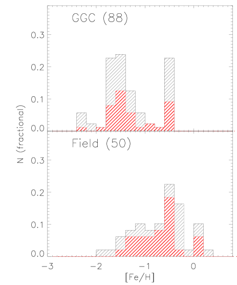
Figure 10: Top: Metallicity distribution of cluster TIICs. The source catalog is on the database by Clement et al. (2001). The iron abundances are based on the metallicity scale by Carretta et al. (2009). Bottom: Same as the top panel, but for Galactic field TIICs. The iron abundances are based on high- and low-resolution spectra The red histogram display the metallicity distribution of WVs only (see text for more details).

Data plotted in the bottom panel of Fig. 10 show that field TIICs cover a broad range in metallicity, from [Fe/H]$\sim$–2 to [Fe/H]$\sim$0.3. The distribution appears to be similar to field RRLs (Magurno et al. 2018; Fabrizio et al. 2019), suggesting a similar evolutionary channel. Moreover, BLHs, WVs and RVTs appear to have very similar metallicity distributions. Recent spectroscopic investigations based on 10 objects suggested that short-period (P$<$3 days) TIICs are separated into metal-rich ([Fe/H]$\gtrsim$–0.5 dex) labeled as BLHs and metal-poor (–2.0$\lesssim$[Fe/H]$\lesssim$–1.5), labeled as UY Eri (UYE) stars (Kovtyukh et al. 2018). Moreover, it was also suggested that field WVs are more metal-poor than –0.3 dex, while the current sample is suggesting a metallicity distribution approaching, within the errors, either solar or super solar iron abundances.

The elemental abundances of TIICs have a long-standing record. Dating back to more than half century ago, Rodgers & Bell (1968) and later on Luck & Bond (1989) found that TIICs are deficient in s-process elements. More recently, Maas et al. (2007) found solid evidence of a contamination with 3$\alpha$ and CN-cycling products in the CNO abundances of field BLHs and WVs. Moreover, they found a clear Na overabundance in BLHs, but not in WVs. There is also evidence that [Ca/Fe] and [Ti/Fe] are under-abundant in WVs thus suggesting the possible presence of a gas-dust separation (Wallerstein et al. 2000).

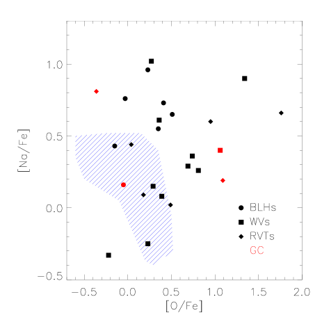
Figure 11: Na-O anticorrelation for field (black) and cluster (red) TIICs. The three different sub-groups are marked with different symbols (see labels). The blue hatched area marks the area covered by cluster stars showing a well defined anti-correlation between Na and O (Gratton et al. 2004a).

To investigate in more detail TIIC chemical peculiarities, and in particular to assess possible differences between field and cluster TIICs, Fig. A.2 shows the measured [Na/Fe] versus [O/Fe] abundance ratios for field and cluster objects. A glance at the data shows that Na and O overabundances in field (black symbols) and cluster (red symbols) TIICs span Oven one dex. There is a marginal evidence for WVs (squares) and RVTs (diamonds) to be more overabundant in O compared to BLHs (circles), while BLHs appear to be more overabundant in Na. However, the sample of TIICs with accurate measurements (two dozen) is too limited to reach firm conclusions. We also note that roughly one third of the current sample overlaps with values typical of cluster stars showing a well-defined anti-correlation between Na and O (Gratton et al. 2004a). Note that the cluster TIICs located in this area is V48 in $\omega$ Cen, and more quantitative discussions concerning the possible difference between first and second generation stars are hampered by the fact that accurate abundances are only available for two out of the seven TIICs present in this cluster.

The above chemical peculiarities for TIICs appear more in context if we take into account the evolutionary properties of their progenitors. Dating back to the seminal theoretical investigations by Giannone & Rossi (1977) and the empirical works by Heber et al. (1986) and Behr (2003), it has become clear that hot and extreme HB stars are affected by gravitational settling and radiative levitation of heavier elements (Cassisi & Salaris 2013). In addition, there is the possibility of having hot helium flashers, stars that do not experience the core helium flash at the tip of the red giant branch, and whose surface abundances are altered by mixing processes during the flash (Castellani & Castellani 1993; D’Cruz et al. 1996; Brown et al. 2000; Cassisi et al. 2003). Recent spectroscopic investigations of extreme HB stars have revealed well defined patterns in their surface chemical composition, that has been altered by chemical element transport processes (Moehler et al. 2011). Moreover, in a recent investigation Latour et al. (2014) found a well defined Helium-Carbon correlation among extreme HB stars in $\omega$ Cen suggesting the occurrence of diffusion mechanisms (Miller Bertolami et al. 2008).

It is clear that cluster TIICs can play a crucial role in addressing some of the current open problems affecting the origin and evolution of TIICs. Indeed for these objects, we have detailed information concerning the age and the chemical composition of their progenitors.

References

- Aparicio & Gallart (2004) Aparicio, A. & Gallart, C. 2004, AJ, 128, 1465
- Baade (1958) Baade, W. 1958, AJ, 63, 207
- Baker & Gough (1979) Baker, N. H. & Gough, D. O. 1979, ApJ, 234, 232
- Beaton et al. (2018) Beaton, R. L., Bono, G., Braga, V. F., et al. 2018, Space Sci. Rev., 214, 113
- Becker et al. (1977) Becker, S. A., Iben, Jr., I., & Tuggle, R. S. 1977, ApJ, 218, 633
- Behr (2003) Behr, B. B. 2003, ApJS, 149, 67
- Bhardwaj et al. (2017) Bhardwaj, A., Macri, L. M., Rejkuba, M., et al. 2017, AJ, 153, 154
- Bono et al. (1997a) Bono, G., Caputo, F., Cassisi, S., Incerpi, R., & Marconi, M. 1997a, ApJ, 483, 811
- Bono et al. (2000) Bono, G., Caputo, F., Cassisi, S., et al. 2000, ApJ, 543, 955
- Bono et al. (1997b) Bono, G., Caputo, F., Castellani, V., & Marconi, M. 1997b, A&AS, 121, 327
- Bono et al. (1999) Bono, G., Caputo, F., Castellani, V., & Marconi, M. 1999, ApJ, 512, 711
- Bono et al. (2008) Bono, G., Caputo, F., Fiorentino, G., Marconi, M., & Musella, I. 2008, ApJ, 684, 102
- Bono et al. (1997c) Bono, G., Caputo, F., & Santolamazza, P. 1997c, A&A, 317, 171
- Bono et al. (2016) Bono, G., d, A., Marconi, M., et al. 2016, Commmunications of the Konkoly Observatory Hungary, 105, 149
- Bono & Marconi (1999) Bono, G. & Marconi, M. 1999, in IAU Symposium, Vol. 190, New Views of the Magellanic Clouds, ed. Y. H. Chu, N. Suntzeff, J. Hesser, & D. Bohlender, 527
- Bono et al. (2013) Bono, G., Salaris, M., & Gilmozzi, R. 2013, A&A, 549, A102
- Bono & Stellingwerf (1994) Bono, G. & Stellingwerf, R. F. 1994, ApJS, 93, 233
- Braga et al. (2019) Braga, V. F., Contreras Ramos, R., Minniti, D., et al. 2019, A&A, 625, A151
- Braga et al. (2015) Braga, V. F., Dall’Ora, M., Bono, G., et al. 2015, ApJ, 799, 165
- Braga et al. (2016) Braga, V. F., Stetson, P. B., Bono, G., et al. 2016, AJ, 152, 170
- Brown et al. (2000) Brown, T. M., Bowers, C. W., Kimble, R. A., Sweigart, A. V., & Ferguson, H. C. 2000, ApJ, 532, 308
- Buchler & Goupil (1988) Buchler, J. R. & Goupil, M.-J. 1988, A&A, 190, 137
- Calamida et al. (2017) Calamida, A., Strampelli, G., Rest, A., et al. 2017, AJ, 153, 175
- Carretta et al. (2009) Carretta, E., Bragaglia, A., Gratton, R., D’Orazi, V., & Lucatello, S. 2009, A&A, 508, 695
- Cassisi & Salaris (2011) Cassisi, S. & Salaris, M. 2011, ApJ, 728, L43
- Cassisi & Salaris (2013) Cassisi, S. & Salaris, M. 2013, Old Stellar Populations: How to Study the Fossil Record of Galaxy Formation
- Cassisi et al. (2003) Cassisi, S., Schlattl, H., Salaris, M., & Weiss, A. 2003, ApJ, 582, L43
- Castellani et al. (2003) Castellani, M., Caputo, F., & Castellani, V. 2003, A&A, 410, 871
- Castellani & Castellani (1993) Castellani, M. & Castellani, V. 1993, ApJ, 407, 649
- Castellani et al. (2006) Castellani, M., Castellani, V., & Prada Moroni, P. G. 2006, A&A, 457, 569
- Castellani et al. (2007) Castellani, V., Calamida, A., Bono, G., et al. 2007, ApJ, 663, 1021
- Castellani et al. (1991) Castellani, V., Chieffi, A., & Pulone, L. 1991, ApJS, 76, 911
- Castelli et al. (1997) Castelli, F., Gratton, R. G., & Kurucz, R. L. 1997, A&A, 318, 841
- Castelli & Kurucz (2003) Castelli, F. & Kurucz, R. L. 2003, in IAU Symposium, Vol. 210, Modelling of Stellar Atmospheres, ed. N. Piskunov, W. W. Weiss, & D. F. Gray, A20
- Chiosi et al. (1993) Chiosi, C., Wood, P. R., & Capitanio, N. 1993, ApJS, 86, 541
- Clement et al. (2001) Clement, C. M., Muzzin, A., Dufton, Q., et al. 2001, AJ, 122, 2587
- Constantino et al. (2016) Constantino, T., Campbell, S. W., Lattanzio, J. C., & van Duijneveldt, A. 2016, MNRAS, 456, 3866
- Cristallo et al. (2009) Cristallo, S., Straniero, O., Gallino, R., et al. 2009, ApJ, 696, 797
- Dalessandro et al. (2016) Dalessandro, E., Lapenna, E., Mucciarelli, A., et al. 2016, ApJ, 829, 77
- Dalessandro et al. (2013) Dalessandro, E., Salaris, M., Ferraro, F. R., Mucciarelli, A., & Cassisi, S. 2013, MNRAS, 430, 459
- D’Cruz et al. (1996) D’Cruz, N. L., Dorman, B., Rood, R. T., & O’Connell, R. W. 1996, ApJ, 466, 359
- Di Criscienzo et al. (2007) Di Criscienzo, M., Caputo, F., Marconi, M., & Cassisi, S. 2007, A&A, 471, 893
- Dorman & Rood (1993) Dorman, B. & Rood, R. T. 1993, ApJ, 409, 387
- Dotter (2008) Dotter, A. 2008, ApJ, 687, L21
- Dziembowski & Cassisi (1999) Dziembowski, W. A. & Cassisi, S. 1999, Acta Astron., 49, 371
- Fabrizio et al. (2019) Fabrizio, M., Bono, G., Braga, V. F., et al. 2019, ApJ, 882, 169
- Feast et al. (2008) Feast, M. W., Laney, C. D., Kinman, T. D., van Leeuwen, F., & Whitelock, P. A. 2008, MNRAS, 386, 2115
- Ferguson et al. (2005) Ferguson, J. W., Alexander, D. R., Allard, F., et al. 2005, ApJ, 623, 585
- Fiorentino et al. (2017) Fiorentino, G., Bellazzini, M., Ciliegi, P., et al. 2017, arXiv e-prints, arXiv:1712.04222
- Fricke et al. (1971) Fricke, K., Stobie, R. S., & Strittmatter, P. A. 1971, MNRAS, 154, 23
- Giannone & Rossi (1977) Giannone, P. & Rossi, L. 1977, Mem. Soc. Astron. Italiana, 48, 776
- Gingold (1974) Gingold, R. A. 1974, ApJ, 193, 177
- Gingold (1976) Gingold, R. A. 1976, ApJ, 204, 116
- Gingold (1985) Gingold, R. A. 1985, Mem. Soc. Astron. Italiana, 56, 169
- Gonzalez & Lambert (1997) Gonzalez, G. & Lambert, D. L. 1997, AJ, 114, 341
- Gonzalez et al. (1997) Gonzalez, G., Lambert, D. L., & Giridhar, S. 1997, ApJ, 479, 427
- Gonzalez & Wallerstein (1994) Gonzalez, G. & Wallerstein, G. 1994, AJ, 108, 1325
- Gonzalez & Wallerstein (1996) Gonzalez, G. & Wallerstein, G. 1996, MNRAS, 280, 515
- Gratton et al. (2004a) Gratton, R., Sneden, C., & Carretta, E. 2004a, ARA&A, 42, 385
- Gratton et al. (2004b) Gratton, R. G., Bragaglia, A., Clementini, G., et al. 2004b, A&A, 421, 937
- Gratton et al. (2003) Gratton, R. G., Carretta, E., Claudi, R., Lucatello, S., & Barbieri, M. 2003, A&A, 404, 187
- Greggio & Renzini (1990) Greggio, L. & Renzini, A. 1990, ApJ, 364, 35
- Groenewegen & Jurkovic (2017a) Groenewegen, M. A. T. & Jurkovic, M. I. 2017a, A&A, 603, A70
- Groenewegen & Jurkovic (2017b) Groenewegen, M. A. T. & Jurkovic, M. I. 2017b, A&A, 604, A29
- Gustafsson et al. (1975) Gustafsson, B., Bell, R. A., Eriksson, K., & Nordlund, A. 1975, A&A, 42, 407
- Gustafsson et al. (2008) Gustafsson, B., Edvardsson, B., Eriksson, K., et al. 2008, A&A, 486, 951
- Guzik et al. (2000) Guzik, J. A., Kaye, A. B., Bradley, P. A., Cox, A. N., & Neuforge, C. 2000, ApJ, 542, L57
- Harris (1981) Harris, H. C. 1981, AJ, 86, 719
- Harris & Wallerstein (1984) Harris, H. C. & Wallerstein, G. 1984, AJ, 89, 379
- Harris (1996) Harris, W. E. 1996, AJ, 112, 1487
- Heber et al. (1986) Heber, U., Kudritzki, R. P., Caloi, V., Castellani, V., & Danziger, J. 1986, A&A, 162, 171
- Iben & Huchra (1970) Iben, Jr., I. & Huchra, J. 1970, ApJ, 162, L43
- Iben & Truran (1978) Iben, Jr., I. & Truran, J. W. 1978, ApJ, 220, 980
- Iglesias & Rogers (1996) Iglesias, C. A. & Rogers, F. J. 1996, ApJ, 464, 943
- Iwanek et al. (2018) Iwanek, P., Soszyński, I., Skowron, D., et al. 2018, Acta Astron., 68, 213
- Johnson & Pilachowski (2010) Johnson, C. I. & Pilachowski, C. A. 2010, ApJ, 722, 1373
- Kippenhahn et al. (1967) Kippenhahn, R., Weigert, A., & Hofmeister, E. 1967, Methods in Computational Physics, 7, 129
- Kovacs & Buchler (1993) Kovacs, G. & Buchler, J. R. 1993, ApJ, 404, 765
- Kovtyukh et al. (2018) Kovtyukh, V., Wallerstein, G., Yegorova, I., et al. 2018, PASP, 130, 054201
- Kurucz (1979) Kurucz, R. L. 1979, ApJS, 40, 1
- Latour et al. (2014) Latour, M., Randall, S. K., Fontaine, G., et al. 2014, ApJ, 795, 106
- Lebzelter & Wood (2016) Lebzelter, T. & Wood, P. R. 2016, A&A, 585, A111
- Lee et al. (1990) Lee, Y.-W., Demarque, P., & Zinn, R. 1990, ApJ, 350, 155
- Lemasle et al. (2015) Lemasle, B., Kovtyukh, V., Bono, G., et al. 2015, A&A, 579, A47
- Luck & Bond (1989) Luck, R. E. & Bond, H. E. 1989, ApJ, 342, 476
- Maas et al. (2007) Maas, T., Giridhar, S., & Lambert, D. L. 2007, ApJ, 666, 378
- Madore (1982) Madore, B. F. 1982, ApJ, 253, 575
- Madore et al. (2017) Madore, B. F., Freedman, W. L., & Moak, S. 2017, ApJ, 842, 42
- Magurno et al. (2019) Magurno, D., Sneden, C., Bono, G., et al. 2019, ApJ, 881, 104
- Magurno et al. (2018) Magurno, D., Sneden, C., Braga, V. F., et al. 2018, ApJ, 864, 57
- Marconi et al. (2018) Marconi, M., Bono, G., Pietrinferni, A., et al. 2018, ApJ, 864, L13
- Marconi et al. (2015) Marconi, M., Coppola, G., Bono, G., et al. 2015, ApJ, 808, 50
- Marconi & Di Criscienzo (2007) Marconi, M. & Di Criscienzo, M. 2007, A&A, 467, 223
- Martínez-Vázquez et al. (2016) Martínez-Vázquez, C. E., Stetson, P. B., Monelli, M., et al. 2016, MNRAS, 462, 4349
- Matsunaga et al. (2013) Matsunaga, N., Feast, M. W., Kawadu, T., et al. 2013, MNRAS, 429, 385
- Matsunaga et al. (2006) Matsunaga, N., Fukushi, H., Nakada, Y., et al. 2006, MNRAS, 370, 1979
- Miller Bertolami et al. (2008) Miller Bertolami, M. M., Althaus, L. G., Unglaub, K., & Weiss, A. 2008, A&A, 491, 253
- Minniti (1995) Minniti, D. 1995, A&A, 303, 468
- Moehler et al. (2011) Moehler, S., Dreizler, S., Lanz, T., et al. 2011, A&A, 526, A136
- Origlia et al. (2014) Origlia, L., Ferraro, F. R., Fabbri, S., et al. 2014, A&A, 564, A136
- Percy et al. (1991) Percy, J. R., Sasselov, D. D., Alfred, A., & Scott, G. 1991, ApJ, 375, 691
- Piatti & Koch (2018) Piatti, A. E. & Koch, A. 2018, ApJ, 867, 8
- Pietrinferni et al. (2006a) Pietrinferni, A., Cassisi, S., Bono, G., et al. 2006a, Mem. Soc. Astron. Italiana, 77, 144
- Pietrinferni et al. (2006b) Pietrinferni, A., Cassisi, S., Salaris, M., & Castelli, F. 2006b, ApJ, 642, 797
- Pilecki et al. (2018) Pilecki, B., Dervi\textcommabelowsoğlu, A., Gieren, W., et al. 2018, ApJ, 868, 30
- Pilecki et al. (2017) Pilecki, B., Gieren, W., Smolec, R., et al. 2017, ApJ, 842, 110
- Pritzl et al. (2002) Pritzl, B. J., Smith, H. A., Catelan, M., & Sweigart, A. V. 2002, AJ, 124, 949
- Pritzl et al. (2003) Pritzl, B. J., Smith, H. A., Stetson, P. B., et al. 2003, AJ, 126, 1381
- Rabidoux et al. (2010) Rabidoux, K., Smith, H. A., Pritzl, B. J., et al. 2010, AJ, 139, 2300
- Rich et al. (2012) Rich, R. M., Origlia, L., & Valenti, E. 2012, ApJ, 746, 59
- Riess et al. (2019) Riess, A. G., Casertano, S., Yuan, W., Macri, L. M., & Scolnic, D. 2019, ApJ, 876, 85
- Ripepi et al. (2019) Ripepi, V., Molinaro, R., Musella, I., et al. 2019, A&A, 625, A14
- Ripepi et al. (2015) Ripepi, V., Moretti, M. I., Marconi, M., et al. 2015, MNRAS, 446, 3034
- Rodgers & Bell (1968) Rodgers, A. W. & Bell, R. A. 1968, MNRAS, 139, 175
- Salaris et al. (2013) Salaris, M., Althaus, L. G., & García-Berro, E. 2013, A&A, 555, A96
- Salaris & Cassisi (2005) Salaris, M. & Cassisi, S. 2005, Evolution of Stars and Stellar Populations (Chichester: John Wiley & Sons, Ltd)
- Salaris et al. (2008) Salaris, M., Cassisi, S., & Pietrinferni, A. 2008, ApJ, 678, L25
- Savino et al. (2015) Savino, A., Salaris, M., & Tolstoy, E. 2015, A&A, 583, A126
- Seaton (2007) Seaton, M. J. 2007, MNRAS, 382, 245
- Soszyński et al. (2019) Soszyński, I., Smolec, R., Udalski, A., & Pietrukowicz, P. 2019, ApJ, 873, 43
- Soszyński et al. (2011) Soszyński, I., Udalski, A., Pietrukowicz, P., et al. 2011, Acta Astron., 61, 285
- Soszyński et al. (2008) Soszyński, I., Udalski, A., Szymański, M. K., et al. 2008, Acta Astron., 58, 293
- Soszyński et al. (2018) Soszyński, I., Udalski, A., Szymański, M. K., et al. 2018, Acta Astron., 68, 89
- Soszyński et al. (2017) Soszyński, I., Udalski, A., Szymański, M. K., et al. 2017, Acta Astron., 67, 297
- Tammann et al. (2003) Tammann, G. A., Sandage, A., & Reindl, B. 2003, A&A, 404, 423
- Torelli et al. (2019) Torelli, M., Iannicola, G., Stetson, P. B., et al. 2019, A&A, 629, A53
- Tuggle & Iben (1973) Tuggle, R. S. & Iben, Jr., I. 1973, ApJ, 186, 593
- Udalski et al. (2015) Udalski, A., Szymański, M. K., & Szymański, G. 2015, Acta Astron., 65, 1
- van Albada & Baker (1973) van Albada, T. S. & Baker, N. 1973, ApJ, 185, 477
- VandenBerg et al. (2013) VandenBerg, D. A., Brogaard, K., Leaman, R., & Casagrande, L. 2013, ApJ, 775, 134
- Vassiliadis & Wood (1993) Vassiliadis, E. & Wood, P. R. 1993, ApJ, 413, 641
- Wagenhuber & Groenewegen (1998) Wagenhuber, J. & Groenewegen, M. A. T. 1998, A&A, 340, 183
- Walker & Terndrup (1991) Walker, A. R. & Terndrup, D. M. 1991, ApJ, 378, 119
- Wallerstein (2002) Wallerstein, G. 2002, PASP, 114, 689
- Wallerstein & Farrell (2018) Wallerstein, G. & Farrell, E. M. 2018, AJ, 156, 299
- Wallerstein & Gonzalez (1996) Wallerstein, G. & Gonzalez, G. 1996, MNRAS, 282, 1236
- Wallerstein et al. (2008) Wallerstein, G., Kovtyukh, V. V., & Andrievsky, S. M. 2008, PASP, 120, 361
- Wallerstein et al. (2000) Wallerstein, G., Matt, S., & Gonzalez, G. 2000, MNRAS, 311, 414
- Weiss & Ferguson (2009) Weiss, A. & Ferguson, J. W. 2009, A&A, 508, 1343
- Zoccali et al. (2017) Zoccali, M., Vasquez, S., Gonzalez, O. A., et al. 2017, A&A, 599, A12