A real-space renormalization-group calculation for the
quantum $\mathbb{Z}_{2}$ gauge theory on a square lattice

Abstract

We revisit Fradkin and Raby’s real-space renormalization-group method to study the quantum $\mathbb{Z}_{2}$ gauge theory defined on links forming a two-dimensional square lattice. Following an old suggestion of theirs, a systematic perturbation expansion developed by Hirsch and Mazenko is used to improve the algorithm to second order in an intercell coupling, thereby incorporating the effects of discarded higher energy states. A careful derivation of gauge-invariant effective operators is presented in the Hamiltonian formalism. Renormalization group equations are analyzed near the nontrivial fixed point, reaffirming old work by Hirsch on the dual transverse field Ising model. In addition to recovering Hirsch’s previous findings, critical exponents for the scaling of the spatial correlation length and energy gap in the electric free (deconfined) phase are compared. Unfortunately, their agreement is poor. The leading singular behavior of the ground state energy density is examined near the critical point: we compute both a critical exponent and estimate a critical amplitude ratio.

I Introduction

We study the quantum Hamiltonian for a two-dimensional $\mathbb{Z}_{2}$ gauge theory on a square lattice using a real-space renormalization-group method. The method, due to Fradkin and Raby, is a gauge-invariance-preserving block-spin algorithm with length rescaling factor two. A variational approximation is made for the ground state of the theory and the Hilbert space is thinned so that low-energy states and long-distance correlations are preserved. Despite the crudeness of the truncation, we demonstrate, without recourse to duality, that spatial correlations decay exponentially in the electric free, or deconfined, phase.

The quantum Hamiltonian may be obtained from classical statistical mechanics by starting with a euclidean three-dimensional $\mathbb{Z}_{2}$ gauge theory on a lattice with anisotropic couplings $\beta_{t}$, along a particular direction chosen as “time,” and $\beta_{s}$ in the orthogonal directions. When the partition function is expressed in terms of a transfer operator, a special limit exists in which the Trotter product formula allows for the transfer operator to be expressed as the exponential of some Hamiltonian $H$. Schultz et al. (1964) This is an infinite-volume limit that is also highly anisotropic and requires $\beta_{t}\to\infty$ and $\beta_{s}\to 0$ such that $\beta_{s}e^{2\beta_{t}}$ remains a fixed and arbitrary dimensionless coupling. Fradkin and Susskind (1978)

At each link $l$ there exists spin-$\tfrac{1}{2}$ operators $\vec{\sigma}_{l}$ obeying the Pauli algebra. Operators belonging to different links commute. The Hamiltonian is

$$H=-h\sum_{l}\sigma^{z}_{l}-J\sum_{p}\Phi_{p},$$ (1)

where $\sigma^{z}_{l}$ measures the discrete electric flux running along link $l$, and $\Phi_{p}=\prod_{l\in\partial p}\sigma^{x}_{l}$ measures the discrete magnetic flux through plaquette $p$.

Local gauge transformations are defined by operators associated to the sites or vertices between links. At such a site $\vec{r}$ in the lattice the generator is

$$G_{\vec{r}}=\prod_{\begin{subarray}{c}\text{links $l$ emerging}\\ \text{from $\vec{r}$}\end{subarray}}\sigma^{z}_{l}.$$ (2)

$G_{\vec{r}}$ commutes with $H$.

order in Hirsch–Mazenko
perturbation theory	$\nu_{t}$	$\nu_{s}$	$\alpha$
first (Refs. Fradkin and Raby, 1979; Mattis and Gallardo, 1980)	0.62	1.20	$-1.02$
second (Ref. Hirsch, 1979 and this work)	0.49	0.65	0.21

Table 1: Critical exponents for the vanishing of the energy gap ($\nu_{t}$), spatial correlation length ($\nu_{s}$), and singularity in the ground state energy ($\alpha$) in the Hirsch–Mazenko perturbation expansion.

The renormalization-group transformation developed by Fradkin and Raby fixed an important shortcoming of previous real-space schemes. Fradkin and Raby (1979) Although blocking spin operators into cells makes a variational approximation to the lattice ground state analytically tractable, such approximations are engineered to preserve the low-energy spectrum without regard for spatial correlations. However, in the Hamiltonian formalism, time and space are treated on very different footings, so one generally needs to ensure that both dimensions scale equally under the renormalization transformation. Consequently, while the gap is well-approximated, (equal-time) correlations exhibit qualitatively incorrect behavior such as power-law decay away from criticality. Fradkin and Raby found that such long-range correlations may be suppressed in the ground state by designing the neighboring block spins to share boundary conditions. This prevents cells from being disconnected because the magnetic flux of one cell is not entirely independent of the flux of its nearest neighbor. They proved that correlation functions decay exponentially in the disordered phase of the one-dimensional transverse field Ising chain. Since the same conclusion holds for the two-dimensional Ising model in a transverse field, Fradkin and Raby invoke duality to argue that it must be true for the $\mathbb{Z}_{2}$ gauge theory in the electric free phase. We shall, in fact, demonstrate this directly using the transformation relations in the gauge theory.

Despite the qualitative success of the real-space renormalization-group transformation, quantitative success eludes this method. In their analysis, Fradkin and Raby used a square block of linear size $2$ (in units of the lattice spacing). Thus, length scales double after each iteration of the blocking transformation. Unfortunately, time does not scale the same way. They find that, even at the fixed point, where one expects the rotational invariance of the classical three-dimensional gauge theory to be fully restored, time increases only by a factor of $1.43$.

Improving upon the lowest order results from the block-spin programme has been a mixed bag, leading some authors to conclude that real-space methods are, at best, semiquantitative. Privman et al. (1991) In studies of the one-dimensional transverse field Ising model enlarging the cell size does improve the computation of critical exponents. Jullien et al. (1978) However, the convergence to exact results are slow and the computation ceases to be analytically tractable beyond cells containing more than a few spins. Certainly, real-space renormalization has not been as successful in producing precise output in the critical regime as other techniques (e.g., epsilon expansion, high-temperature series, Monte Carlo, conformal bootstrap). The difficulty of systematically correcting the variational approximation also casts some doubt as to whether the procedure is physically reasonable—it is hard to judge the efficacy of the approximation based solely on the numerical proximity of exponents as this might be accidental.

It was suggested by Fradkin and Raby that the asymmetric scaling of space and time in their transformation could be remedied by applying a perturbative formalism developed by Hirsch and Mazenko in Ref. Hirsch and Mazenko, 1979. In this approach virtual effects arising from decimated degrees of freedom generate effective operators connecting nearby plaquettes and links. The expansion is organized around a parameter, $g$, such that the original results of Fradkin and Raby are obtained at order $g^{1}$, and quantum fluctuations from truncated cell spectra influence the renormalized Hamiltonian at order $g^{2}$ and beyond by generating new effective interactions. The order $g^{2}$ calculation has been studied by Hirsch in the context of the Ising model. Hirsch (1979) In the present work we show how the same formalism can be applied in the $\mathbb{Z}_{2}$ gauge theory. We find the same results for critical exponents as Hirsch because our effective operators in the lattice gauge theory map into those of the Ising model according to the well-known duality transformation. The results confirm that the scaling of spatial correlations improves significantly in going from order $g^{1}$ to $g^{2}$. We understand this to be due to the inclusion of more delocalized operators in the effective Hamiltonian. Unfortunately, the gap critical exponent worsens significantly. We understand this to mean that the parameter $g$ does not encode small corrections to the variational ground state. This is unsurprising since $g$ is not related a priori to the dimensionless ratio $J/h$. Rather, $g$ arises due to an artificial separation of the Hamiltonian into intra- and intercell terms. Therefore, including higher-order-in-$g$ corrections will not necessarily improve the estimate for the gap.

The main objective of this article is to explore Hirsch and Mazenko’s renormalization-group perturbation method at second order in the real-space framework of Hamiltonian lattice gauge theory. To the best of our knowledge, a calculation based on such an approach has not been presented in the literature. The quantitative improvements for critical exponents garnered in this approach are modest compared to prior real-space findings—they are not, by any means, state-of-the-art. We are able to cross-check our calculations with Hirsch’s for the transverse field Ising model. The existence of a dual model without local symmetry is obviously helpful, but not requisite.

This article is organized as follows. In Section II we review the basic formalism of Fradkin and Raby’s real-space renormalization-group approach and how it fits into the perturbation theory of Hirsch and Mazenko. In Section III we pause to prove the exponential decay of spatial correlations between $\mathbb{Z}_{2}$ magnetic monopoles in the ground state of the electric free phase. Our results near and at criticality are presented in Section IV. A brief discussion is given in Section V. The technical aspects of the renormalization calculation are explained in detail in the appendix.

II Methodology

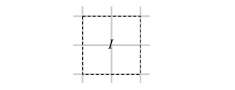
Figure 1: The cell $I$ consists of four plaquettes.

Following Fradkin and Raby, partition the lattice into regular, repeating square cells $I$ each comprised of four plaquettes $p$. See Fig. 1. A given link $l$ belonging to a cell is classified into one of two groups: internal (denoted by a dedicated index $i$) corresponding to the four central links situated inside the cell, and external (denoted by a dedicated index $b$) corresponding to the eight boundary links around the edge of the cell. Let each cell have its own cellular Hamiltonian given by

$$H_{I}=-h\sum_{i\in I}\sigma^{z}_{i}-J\sum_{p\in I}\Phi_{p}.$$ (3)

Since only the transverse field operators $\sigma^{z}_{i}$ of the four internal links are included, only these degrees of freedom act quantumly. The operators $\sigma^{x}_{b}$ of the eight external links behave classically and their eigenvalues serve as boundary conditions on the cell spectrum. We denote external link eigenstates and eigenvalues as

$$\sigma^{x}_{b}|x_{b}\rangle=x_{b}|x_{b}\rangle,\quad x_{b}=\pm 1.$$ (4)

Since cell $I$ contains four qubits and eight bits, and the cell Hamiltonian commutes with a generator of $\mathbb{Z}_{2}$ gauge transformations located at its center site, the cell Hilbert space has dimensionality $2^{4-1}=8$ per boundary configuration. The spectrum is easily worked out analytically. Cell eigenstates depend parametrically on the $x_{b}$ around the boundary of the cell. Let us denote the cell ground state as $|0(\{x_{b}\})\rangle_{I}$. Gauge symmetry constrains its energy eigenvalue $\epsilon^{0}_{I}$ to depend only on the product $\Phi_{I}=\prod_{b\in I}x_{b}$.

Define interactions by

$$V=-h\sum_{I}\sum_{b\in I}\sigma^{z}_{b},$$ (5)

where it is understood that links are not repeated in the sum. The original lattice Hamiltonian is then

$$H=\sum_{I}H_{I}+gV,$$ (6)

where the intercell coupling $g$ has been introduced to aid in organizing a perturbation expansion—its value is ultimately set to 1.

The goal is to construct a renormalized Hamiltonian $H^{\text{ren}}$ governing a new set of spin-$\tfrac{1}{2}$ operators $\{X_{B},\,Z_{B}\}$ again obeying the Pauli algebra and defined on links $B$ corresponding to the sides of the cells $I$. The renormalized electric and magnetic flux operators $Z_{B}$ and $\prod_{B\in I}X_{B}$ will then come with renormalized couplings $h^{\prime}$ and $J^{\prime}$, respectively. But we also expect that more complicated gauge-invariant operators are generated. This will proliferate more couplings. $H^{\text{ren}}$ is constructed such that, for an arbitrary configuration of the external link eigenvalues, its lowest eigenvalue is identical to that of $H$. At $g=0$ this is done by projecting $H$ onto a subspace spanned by states $|n\rangle$ which are formed from tensor products over all cells $I$ of $|0(\{x_{b}\})\rangle_{I}$ and the $|x_{b}\rangle$ (without repetition). Such states have energy $\epsilon_{n}=\sum_{I}\epsilon^{0}_{I}(\Phi_{I})$. The truncated Hilbert space is spanned by states $|\mu_{n}\rangle$ which are simply products of the $|x_{b}\rangle$. In essence, the internal links are decimated by the truncation. At the surviving links we define new operators $\mu^{x}_{b}=(|+\rangle\langle+|-|-\rangle\langle-|)_{b}$ and $\mu^{z}_{b}=(|+\rangle\langle-|+|-\rangle\langle+|)_{b}$. Then, for each pair of contiguous links $b$ and $b^{\prime}$ in the lattice, we define renormalized operators $X_{B}=\mu_{b}^{x}\mu_{b^{\prime}}^{x}$ and $Z_{B}=(\mu_{b}^{z}+\mu_{b^{\prime}}^{z})/2$.

There is a set of vectors $\{|\alpha\rangle\}$ much larger than and orthogonal to the set $\{|n\rangle\}$ that, when combined with $\{|n\rangle\}$, span the original Hilbert space. We construct $|\alpha\rangle$ similarly to $|n\rangle$ except that one or more cell eigenstates must be chosen in an excited cell state. For $g>0$ the lowest eigenvalue of $H$ and $\sum_{I}H_{I}$ are not the same. Correcting this order by order in $g$ constrains the renormalized Hamiltonian to have the form Hirsch and Mazenko (1979)

$$H^{\text{ren}} = H^{(0)}+gH^{(1)}+g^{2}H^{(2)}+\dotsb,$$ (7a)

$$H^{(0)} = \sum_{n}\epsilon_{n}|\mu_{n}\rangle\langle\mu_{n}|$$ (7b)

$$H^{(1)} = \sum_{n,n^{\prime}}\langle n^{\prime}|V_{\sigma}|n\rangle|\mu_{n}\rangle\langle\mu_{n^{\prime}}|$$ (7c)

$$H^{(2)} = \tfrac{1}{2}\sum_{n,n^{\prime}}\sum_{\alpha}\langle n^{\prime}|V_{\sigma}|\alpha\rangle\langle\alpha|V_{\sigma}|n\rangle$$ (7d)

$$\times\Bigl{(}\frac{1}{\epsilon_{n}-\epsilon_{\alpha}}+\frac{1}{\epsilon_{n^{\prime}}-\epsilon_{\alpha}}\Bigr{)}|\mu_{n}\rangle\langle\mu_{n^{\prime}}|.$$

The detailed computation of these terms may be found in the appendix.

III Proof of exponential decay

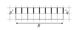
Figure 2: A correlation function of disorder operators at plaquettes at $p$ and $q$ separated by a line $\gamma$ of $R+1$ vertical links (bold). Attached to each one of these links $l$ is a transverse field operator $\sigma^{z}_{l}$. One iteration of the decimation procedure (cells are shown dashed) reduces the separation to $R/2$. Links on the edges of the cells are boundary links and operators living on these links do not act directly on the Hilbert space of the cell.

Let $\lambda=J/h$. The electric free phase—the ground state in which lines of electric flux can meander throughout the lattice without energy cost—corresponds to $\lambda\gg 1$. Denote the ground state of the lattice Hamiltonian by $|\text{gs}_{\lambda}\rangle$. ’t Hooft disorder operators—which are string-like yet still local—create and annihilate magnetic monopoles. Their correlation function, when separated by a row of $R=2^{n}$ plaquettes, is given by

$$C_{\lambda}(R)=\langle\text{gs}_{\lambda}|\prod_{l\in\gamma}\sigma^{z}_{l}|\text{gs}_{\lambda}\rangle,$$ (8)

where $\gamma$ is the set of $R+1$ vertical links separating the two plaquettes. See Fig. 2. Fradkin and Raby’s decimation procedure amounts to the approximate replacement

$$|\text{gs}_{\lambda}\rangle\simeq\prod_{I}|0(\{x_{b}\})\rangle_{I}|\text{gs}_{\lambda^{\prime}}\rangle.$$ (9)

Here $|\text{gs}_{\lambda^{\prime}}\rangle$ is the ground state of $H^{\text{ren}}$ with $\lambda^{\prime}=J^{\prime}/h^{\prime}$, which now has a fourth as many plaquettes. This is a truncation of the the original Hilbert space to a subspace of states that may be expressed solely in terms of boundary link eigenstates $|x_{b}\rangle$. Substitution gives

$$C_{\lambda}(R)=\langle\text{gs}_{\lambda^{\prime}}|\prod_{b}\sigma^{z}_{b}\prod_{I=1}^{R/2}\langle 0|\sigma^{z}_{i}|0\rangle_{I}|\text{gs}_{\lambda^{\prime}}\rangle.$$ (10)

The appendix contains the explicit cell ground state wavefunction, Eq. (55) or Eq. (57), and representation of the internal $\sigma^{z}_{i}$ matrices, Eq. (53), needed to compute the cell matrix element. Irrespective of the choice for $i$, the matrix element turns out to depend only on the sign of the magnetic flux,

$$\langle 0|\sigma^{z}_{i}|0\rangle_{I}=\tfrac{1}{2}(A_{\lambda}^{-}+A_{\lambda}^{+})\mathrm{1\!\!1}_{I}-\tfrac{1}{2}(A_{\lambda}^{-}-A_{\lambda}^{+})\Phi_{I},$$ (11a)

where

$$A_{\lambda}^{+} = \frac{(1-\lambda^{2}+(1+\lambda^{4})^{1/2})(1+\lambda^{2}+(1+\lambda^{4})^{1/2})^{1/2}}{2\sqrt{2}(1+\lambda^{4})^{1/2}},$$ (11b)

$$A_{\lambda}^{-} = \frac{1}{2}\Bigl{(}1+\frac{1}{(1+\lambda^{2})^{1/2}}\Bigr{)}.$$ (11c)

To $O(g^{1})$, the renormalized couplings $J^{\prime}$ and $h^{\prime}$ may be read off from Eqs. (67c) and (68e), respectively. For an initial choice of $\lambda\gg 1$, there is the asymptotic equivalence

$$\lambda^{\prime}\approx 2\lambda.$$ (12)

Since the renormalized coupling increases with iteration, the ground state has no magnetic energy and the operator $\Phi_{I}$ evaluates to $+1$. In terms of renormalized link operators, this yields the multiplicative recursion relation

$$C_{\lambda}(R)\approx(A^{+}_{\lambda})^{R/2}C_{\lambda^{\prime}}(R/2).$$ (13)

Iterating $n$ times starting from $\lambda_{0}$,

$$C_{\lambda_{0}}(2^{n})=(A^{+}_{\lambda_{0}})^{2^{n-1}}(A^{+}_{\lambda_{1}})^{2^{n-2}}\dotsb(A^{+}_{\lambda_{n-1}})^{2^{n-n}}C_{\lambda_{n}}(1).$$ (14)

Substituting $A^{+}_{\lambda}\approx 1/2\lambda$ and $\lambda_{n}\approx 2^{n}\lambda_{0}$ yields

$$C_{\lambda_{0}}(2^{n})\approx\frac{2^{n}}{(4\lambda_{0})^{2^{n}-1}}C_{2^{n}\lambda_{0}}(1).$$ (15)

But $C_{\lambda}(1)\sim\lambda^{-1}$ up to some constant factor, so

$$C_{\lambda_{0}}(R)\sim\frac{4R}{(4\lambda_{0})^{R}}\propto\exp(-R\log(4\lambda_{0})).$$ (16)

IV Results

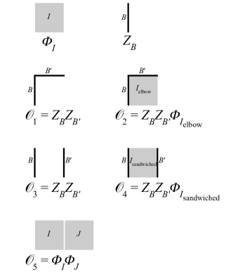
Figure 3: Effective operators present in renormalized Hamiltonian $H^{\text{ren}}$ to second order in the intercell coupling $g$. These are dual to the operators found by Hirsch in his study of the two-dimensional Ising model in a transverse field. Hirsch (1979)

Our main technical achievement is the explicit expression for the renormalized Hamiltonian calculated from Eq. (7). The details of the calculation are given in the appendix. The reader interested only in the final form of $H^{\text{ren}}$ can see the precise operators in Eq. (125), although several definitions needed to understand the coefficients of these operators are scattered throughout the appendix. It turns out that five new effective operators are created in addition to the effective electric flux $hZ_{B}$ on each link $B$, and effective magnetic flux $J\Phi_{I}$ on each cell $I$. We denote these new operators as $K_{\alpha}\mathcal{O}_{\alpha}$ for $\alpha=1,\dotsc,5$. See Fig. 3. Also present is the identity $F\mathrm{1\!\!1}_{I}$ on each cell $I$.

IV.1 Critical point

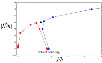
Figure 4: Plot of discrete RG flows beginning from the $\vec{K}/h=0$ axis projected into the $(J/h,|\vec{K}/h|)$ plane (color online). The nontrivial fixed point is indicated by a black triangle. An initial coupling just above the critical value initiates a flow in which $J/h$ tends to grow without bound (blue dots). An initial coupling just below the critical value produces a flow that terminates near the origin (red squares). The critical surface lies in-between these flows, and connects the critical coupling to the nontrivial fixed point.

In the appendix we study numerically the recursion relations for the operator coefficients $h$, $J$, $K_{\alpha}$, and $F$. Following Fradkin and Raby, we adopt $h$ as an energy scale and consider the dimensionless couplings $(J/h,K_{\alpha}/h)$ packaged into a six-dimensional vector. Iterations of the recursion relations produce a sequence of points in this vector space (a discrete “RG flow”) that describes Hamiltonians defined over successively coarser lattices. We are interested in flows that begin on the axis $(J/h,\vec{0})$. Our numerical analysis was implemented in Mathematica 10. One way to visualize the flow is shown in Fig. 4, where the sequence of points in the full six-dimensional space has been projected down to the plane $(J/h,|\vec{K}/h|)$. On the line given by $\vec{K}/h=0$, there exists a critical coupling $(J/h)_{\text{c}}=3.56895$ for which the flow converges onto a nontrivial fixed point $(J/h,\vec{K}/h)_{*}$. This fixed point, whose full coordinates are given in the appendix, was located using Newton’s root-finding method yielding very fast convergence in only several iterations starting from the initial point $(J/h,\vec{K}/h)=(3.3,\vec{0})$. Our fine-tuning estimate for the critical coupling was obtained by searching for the flow that spent the greatest number of steps near the fixed point within some tolerance.

Generically, for $J/h\neq(J/h)_{\text{c}}$, flows eventually veer away from the fixed point and tend toward either the origin or grow unbounded as suggested in Fig. 4. Thus, the nontrivial fixed point is unstable and infrared-repulsive, whilst the trivial fixed points at the origin and infinity are stable and infrared-attractive. We note that couplings in the electric free phase for $J/h$ slightly larger than $(J/h)_{\text{c}}$ give rise to flows in which $J/h$ gets extremely large relative to $|\vec{K}/h|$, and while there appears to be no bound on this growth, the sign of $J/h$ eventually alternates which calls into question the asymptotic reliability of the recursion relation.

In the neighborhood of the nontrivial fixed point there is a linear space with a single relevant scaling variable that we call $u_{1}$. Iterations of the recursion relations renormalize $u_{1}$ to $\Lambda_{1}u_{1}$, where $\Lambda_{1}>1$ is an eigenvalue computed in the appendix.

IV.2 Energy gap

Consider the electric free phase in which $J/h$ is only slightly greater than $(J/h)_{\text{c}}$. The flow is observed to behave as follows: a small and finite number of steps $N_{1}$ brings the flow from $(J/h,\vec{0})$ into the neighborhood of the nontrivial fixed point; for some large, but finite, number of steps $N_{2}$, the flow dawdles and remains quite close to the fixed point; further steps finally allow the flow to escape this region and head off to infinity. Numerical analysis shows that whilst the five couplings $K_{\alpha}/h$ remain of order one, the coupling $J/h$ grows without bound. This is expected since the trivial fixed point at infinity should describe the deconfined phase of the lattice gauge theory with infinitely heavy magnetic monopoles. So now consider the recursion relations just for the coefficients $h$ and $J$, which may be expressed in the form

$$h^{\prime} = h\zeta(J/h,\vec{K}/h),$$ (17a)

$$J^{\prime} = J\eta(J/h,\vec{K}/h).$$ (17b)

Specifically, the function $\zeta$ is given by dividing the right-hand side of Eq. (125b) by $h$, and the function $\eta$ is given by dividing the right-hand side of Eq. (125c) by $J$. Numerical evidence suggests that repeated iterations cause $\zeta$ to approach some number less than 1, and $\eta$ to approach 1. Therefore, in the limit of infinitely many renormalization-group iterations the coefficient $h$ will vanish and only $J$ will remain. Thus, the original Hamiltonian defined on the fine lattice will exhibit the same energy gap as a Hamiltonian defined on the coarse lattice containing only the operators $\sum_{I}\Phi_{I}$. Since the latter theory is weakly coupled, it may be analyzed perturbatively.

The ground state is characterized by the absence of magnetic flux for all plaquettes (i.e., $\Phi_{I}=+1$ for all $I$). The lowest energy excitation creates a unit of magnetic flux on a single plaquette. The energy of the first excited state (relative to the ground state) is $G\simeq 2J_{N}$, where $N$ indicates the total number of iterations of the recursion relations. Since $J_{N}=J_{0}\prod_{n=0}^{N-1}\eta(J_{n}/h_{n},\vec{K}_{n}/h_{n})$, we need only keep a record of the point sequence along the flow in order to calculate the gap. However, close to criticality the product may be decomposed as

$$G\simeq 2J_{0}\prod_{n=0}^{N_{1}-1}\eta\prod_{n=N_{1}}^{N_{1}+N_{2}}\eta\prod_{n=N_{1}+N_{2}}^{N}\eta.$$ (18)

The first product in Eq. (18) corresponds to the inflow. It will be analytic in the difference $J/h-(J/h)_{\text{c}}$. The last product corresponds to the outflow and therefore we expect it asymptotes to the value 1. However, the middle product corresponds to the dawdle near the fixed point. We can evaluate $\eta$ at the fixed point—this approximation gets better the closer the flow starts to criticality. The number $N_{2}$ may be estimated by asking how many steps need to be taken to multiplicatively renormalize the relevant scaling variable $u_{1}$—which we assume is exceedingly small at step $N_{1}$—into an arbitrary, but fixed and small number $U_{1}$ for which the linearized approximation to the recursion relations is still valid. This condition is

$$U_{1}=\Lambda_{1}^{N_{2}}u_{1}\implies N_{2}=\log(U_{1}/u_{1})/\log\Lambda_{1}.$$ (19)

Hence,

$$\text{nonanalytic part of $G$}\sim\eta((J/h,\vec{K}/h)_{*})^{N_{2}}.$$ (20)

Since $u_{1}$ arises from the inflow and $N_{1}$ is finite, it follows that $u_{1}$ itself is some analytic function of $J/h-(J/h)_{\text{c}}$. Finally,

$$\text{nonanalytic part of $G$}\sim(J/h-(J/h)_{\text{c}})^{\nu_{t}},$$ (21)

where

$$\nu_{t}=\frac{-\log\eta((J/h,\vec{K}/h)_{*})}{\log\Lambda_{1}}\simeq 0.49.$$ (22)

Obtaining this critical exponent, which was not computed in Ref. Hirsch, 1979, was one of the original motivations for this work.

IV.3 Spatial correlation length

In the electric free phase, the correlation function of disorder operators given by Eq. (8) ought to have a correlation length $\xi$ that diverges as $J/h$ approaches $(J/h)_{\text{c}}$ from above. After some large number $N$ of decimations, the dimensionless correlation length will be an order one number because the flow will be far from the neighborhood of the fixed point where the linearized recursion relations hold. Therefore, the part of $N$ that depends on the reduced coupling $J/h-(J/h)_{\text{c}}$ must be the same as $N_{2}$ as estimated in Eq. (19). Since our renormalization scale factor is $2$,

$$\xi\sim 2^{N}\sim(J/h-(J/h)_{\text{c}})^{\nu_{s}},$$ (23)

where

$$\nu_{s}=\frac{\log 2}{\log\Lambda_{1}}\simeq 0.65.$$ (24)

IV.4 Ground state energy

From the coefficient of the identity operator on each cell it is possible to represent the ground state energy by the expression

$$E_{\text{gs}}(J/h,\vec{K}/h)=\lim_{n\to\infty}F^{(n)}\frac{N_{\text{plaq}}}{4^{n}},$$ (25)

where the superscript ⁽ⁿ⁾ denotes the $n$th iteration of the recursion relation given by Eq. (125i). The case $n=0$ indicates the original bare coupling. For instance, $h^{(0)}=h$. Define the energy density by $\varepsilon_{\text{gs}}=E_{\text{gs}}/N_{\text{plaq}}$. Rather than a limit, let us express the ground state energy density as an infinite sum. For clarity, we write the six-dimensional vector of dimensionless couplings as $\kappa^{(n)}=(J^{(n)}/h^{(n)},\vec{K}^{(n)}/h^{(n)})$. Knowing that the recursion relation for $F$, Eq. (125i), takes the form

$$F^{(n+1)}=4F^{(n)}+h^{(n)}\Delta(\kappa^{(n)}),$$ (26)

where $\Delta$ is an analytic function of its argument, we obtain

$$\varepsilon_{\text{gs}}(\kappa^{(0)})=\sum_{n=0}^{\infty}\frac{1}{4^{n+1}}h^{(n)}\Delta(\kappa^{(n)}).$$ (27)

We have assumed that $F^{(0)}=0$. Since the recursion relation for $h$, Eq. (125b), takes the form

$$h^{(n+1)}=h^{(n)}\zeta(\kappa^{(n)}),$$ (28)

it follows that

$$h^{(n)}=h^{(0)}\zeta(\kappa^{(0)})\zeta(\kappa^{(1)})\dotsb\zeta(\kappa^{(n-1)}).$$ (29)

Therefore, in Eq. (27), specification of $\kappa^{(0)}$ completely determines the right-hand side since the recursion relations may be applied to to obtain $\kappa^{(1)}$, $\kappa^{(2)}$, etc. Following Ref. Mattis and Gallardo, 1980, Eq. (27) may be written

$$\varepsilon_{\text{gs}}(\kappa^{(0)})=\tfrac{1}{4}h^{(0)}\Delta(\kappa^{(0)})+\tfrac{1}{4}\zeta(\kappa^{(0)})\biggl{[}\tfrac{1}{4}h^{(0)}\Delta(\kappa^{(1)})+\tfrac{1}{4^{2}}h^{(0)}\zeta(\kappa^{(1)})\Delta(\kappa^{(2)})+\tfrac{1}{4^{3}}h^{(0)}\zeta(\kappa^{(1)})\zeta(\kappa^{(2)})\Delta(\kappa^{(3)})+\dotsb\biggr{]}.$$ (30)

Notice that the bracketed term in Eq. (30) is just the right-hand side of Eq. (27) but started at the point $\kappa^{(1)}$. Thus, we arrive at a recursion relation satisfied by the ground state energy density, Mattis and Gallardo (1980)

$$\varepsilon_{\text{gs}}(\kappa^{(0)})=\tfrac{1}{4}h^{(0)}\Delta(\kappa^{(0)})+\tfrac{1}{4}\zeta(\kappa^{(0)})\varepsilon_{\text{gs}}(\kappa^{(1)}).$$ (31)

We are interested in extracting the leading singular behavior of the ground state energy density as the critical point is approached. Since $\Delta$ is differentiable, even at the fixed point, Eq. (31) implies the following homogeneous transformation law for the singular part of $\varepsilon_{\text{gs}}$,

$$\varepsilon_{\text{gs}}^{\text{sing}}(\kappa)=\frac{1}{4}\zeta(\kappa)\varepsilon_{\text{gs}}^{\text{sing}}(\kappa^{\prime}).$$ (32)

Close to the fixed point, we can write this using scaling variables. Ignoring irrelevant variables and iterating $n$ times,

$$\varepsilon_{\text{gs}}^{\text{sing}}(u_{1})=4^{-n}\prod_{r=0}^{n-1}\zeta(\Lambda_{1}^{r}u_{1})\varepsilon_{\text{gs}}^{\text{sing}}(\Lambda_{1}^{n}u_{1}).$$ (33)

Since $u_{1}$ grows under iteration we need to apply a stopping condition. We take $n=N_{2}$ as specified by Eq. (19). If $\Lambda_{1}^{r}u_{1}$ remains small, then we may approximate each $\zeta$ by its value at the fixed point $u_{1}=0$. Then

$$\varepsilon_{\text{gs}}^{\text{sing}}(u_{1})\approx(4/\zeta(0))^{-n}\varepsilon_{\text{gs}}^{\text{sing}}(U_{1})\sim u_{1}^{\frac{\log(4/\zeta(0))}{\log\Lambda_{1}}}.$$ (34)

Finally,

$$\text{singular part of $\varepsilon_{\text{gs}}$}\sim|J/h-(J/h)_{\text{c}}|^{2-\alpha},$$ (35)

where

$$\alpha=2-\frac{\log(4/\zeta(0))}{\log\Lambda_{1}}\simeq 0.21.$$ (36)

A direct numerical calculation of Eq. (27) at the critical coupling $(J/h)_{\text{c}}$ produces $\varepsilon_{\text{gs}}\simeq-3.718h^{(0)}$.

IV.5 A critical amplitude ratio

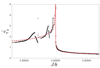
Figure 5: A plot of a numerical calculation of $-\partial^{2}\varepsilon_{\text{gs}}/\partial(J/h)^{2}$. It diverges at the critical coupling $(J/h)_{\text{c}}=3.56895$. Fits to the leading singular behavior are shown as dashed red lines (color online). The numerous local peaks and valleys below the critical coupling are spurious artifacts of our numerical method and should be ignored.

We also studied the divergence of the second derivative of the ground state energy density with respect to $J/h$, denoted $\varepsilon_{\text{gs}}^{\prime\prime}$, in a small region around the critical coupling. A plot of this divergence is visible in Fig. 5 as the prominent spike. The main difficulty in obtaining these values, besides discretization error associated with differentiating, is the inability to evaluate Eq. (27) to arbitrarily high $n$. Our renormalization group transformation $\kappa^{(n)}\to\kappa^{(n+1)}$ cannot be iterated indefinitely without running into a nonsensical value for $J/h$ (e.g., negative values). In practice, we could iterate the flow between 10 and 20 steps, more steps being possible the closer $J/h$ begins to the true critical coupling.

The leading singular behavior in $\varepsilon_{\text{gs}}$ comes from that part of the sum in Eq. (27) corresponding to the renormalization flow along the outflow trajectory (see Fig. 11) Cardy (1996). Since the flow away from the fixed point is different for the two phases of the gauge theory, we expect the amplitude $A$ to be different for $J/h>(J/h)_{\text{c}}$ and $J/h<(J/h)_{\text{c}}$. We may write

$$\text{leading singular part of $\varepsilon_{\text{gs}}$}\sim A_{>,<}|J/h-(J/h)_{\text{c}}|^{2-\alpha}.$$ (37)

The amplitude ratio $A_{>}/A_{<}$ is a universal quantity, but unlike critical exponents, it depends on the entire flow, not just the linearized flow in the vicinity of the fixed point.

We applied a naive procedure to obtain a cursory estimate for the amplitudes. After transforming data to the form $(\log|J/h-(J/h)_{\text{c}}|,\,\log\varepsilon_{\text{gs}}^{\prime\prime})$, we made a least-squares fit to the line $y=b_{0}-\alpha x$, where $b_{0}$ is the single free parameter and $\alpha$ is constrained to be the value in Eq. (36). We remark that, even with a two-parameter fit like $y=b_{0}-b_{1}x$, the slope parameter $b_{1}$ comes within $10\%$ of $\alpha$. Notice that we completely ignore correction-to-scaling terms in these fits. We obtain $b_{0}^{>}=-2.368$ and $b_{0}^{<}=-1.036$. Then

$$A_{>}/A_{<}=\exp(b_{0}^{>}-b_{0}^{<})\simeq 0.26.$$ (38)

For comparison, the ratio of specific heat amplitudes in the three-dimensional Ising universality class is known to be about 0.52. Privman et al. (1991)

order in Hirsch–Mazenko
perturbation theory	$(J/h)_{\text{c}}$	$E_{\text{gs}}/hN_{\text{plaq}}$
first (Refs. Fradkin and Raby, 1979; Mattis and Gallardo, 1980)	3.28	$-3.376$
second (Ref. Hirsch, 1979 and this work)	3.57	$-3.718$

Table 2: Critical coupling $(J/h)_{\text{c}}$ and critical ground state energy per plaquette $E_{\text{gs}}/hN_{\text{plaq}}$ in the Hirsch–Mazenko perturbation expansion.

V Discussion

Using Hirsch–Mazenko perturbation theory we have calculated some critical properties of the quantum $\mathbb{Z}_{2}$ gauge theory on a square lattice. Universal critical exponents are given in Table 1 while nonuniversal data are collected in Table 2. Most indications are that the second-order theory is an improvement over the first-order theory.

It is known from Monte Carlo simulations of the simple cubic Ising model that the critical inverse temperature is $K_{\text{c}}\simeq 0.22$ and the critical exponent for the correlation length is $\nu_{\text{Ising}}\simeq 0.63$ Ferrenberg et al. (2018). Hyperscaling then implies that the critical exponent for the specific heat is $\alpha_{\text{Ising}}=2-3\nu_{\text{Ising}}\simeq 0.11$. Using duality we are able to transfer these values over to the gauge theory: the critical coupling ought to be $(J/h)_{\text{c}}=K_{\text{c}}^{-1}\simeq 4.51$, the critical exponents for the energy gap and spatial correlation length—equal due to rotational invariance at the critical point—ought to be $\nu_{s}=\nu_{t}=\nu_{\text{Ising}}\simeq 0.63$, and the critical exponent for the leading singular behavior of the ground state energy ought to be $\alpha=\alpha_{\text{Ising}}\simeq 0.11$.

Most of our second-order results are closer to these expected values than the first-order results. Of particular note is that $\nu_{s}$ and $\alpha$, which we stress were computed independently, both improved dramatically at second order. To wit, $\alpha$ made a qualitative switch from negative to positive!

Furthermore, at the fixed point, we find that the reciprocal of the gap energy scales, under a renormalization transformation, by a factor of $1/\eta((J/h,\vec{K}/h)_{*})\simeq 1.68$. This is certainly closer to the spatial scale factor of $2$ than the $O(g^{1})$ result of $1.43$. This supports Fradkin and Raby’s suggestion that systematic improvement is possible using a perturbative framework like Hirsch and Mazenko’s.

In order to evaluate the accuracy of the critical ground state energy density, we may use a duality relation between quantum Hamiltonians for the two-dimensional $\mathbb{Z}_{2}$ lattice gauge theory (“LGT”) and the two-dimensional transverse field Ising model (“TFIM”) Kogut (1979). If $\lambda=J/h$ and $E$ is any eigenvalue, then $E_{\text{LGT}}(\lambda)=\lambda E_{\text{TFIM}}(\lambda^{-1})$. Using the critical data in Table 2, the critical ground state energy per spin in the TFIM is approximately $-1.03$ (first order) and $-1.04$ (second order). A numerical calculation of the lowest eigenvalue of the TFIM Hamiltonian on a $4\times 4$ lattice evaluated at coupling $K_{c}$ yields a ground state energy per spin of $-1.02$. The agreement is decent.

Unfortunately, not all Hirsch–Mazenko perturbative corrections are improvements. There is a clear worsening of the gap critical exponent: the second-order value for $\nu_{t}$ is much worse than its first-order value. This suggests that the artificial separation of the Hamiltonian given by Eq. (6) is not a small correction to the variational ground state energy.

cell size	$(J/h)_{\text{c}}$	$\nu_{t}$	$\nu_{s}$
$2\times 2$	3.280	0.622	1.197
$3\times 3$	3.036	0.624	1.006
$4\times 4$	2.970	0.627	0.924

Table 3: Critical coupling and exponents at $O(g^{1})$ in the Hirsch–Mazenko perturbation expansion for different cell sizes. These are most easily computed from the transverse field Ising model via duality. Drell et al. (1977); Sólyom (1981)

One may straightforwardly improve $\nu_{t}$ by enlarging the cell size. For instance, we have done an $O(g^{1})$ analysis using $3\times 3$ and $4\times 4$ cells. Our results are summarized in Table 3. There is modest improvement after increasing the cell Hilbert space dimensionality from $2^{4}$ to $2^{9}$ and then to $2^{16}$, indicating that the variational approximation is a little better.

What lessons and future directions does our work suggest? We have confirmed Fradkin and Raby’s speculation that Hirsch–Mazenko perturbation theory can be applied to a lattice gauge theory and that a second-order correction of their renormalization transformation does lead to some qualitative improvements in the critical behavior. However, it is clear that precisely approximating critical exponents is not a strength of the real-space method. The attractiveness of the method is tempered by the fact that some critical exponents (e.g., $\nu_{t}$) can get worse. Therefore, the most promising and fruitful use of this work would be to guide explorations of more complicated gauge-invariant Hamiltonians in two dimensions. Preserving gauge invariance at successive steps in the renormalization process is nontrivial, but we have demonstrated explicitly how it happens for the simplest gauge group.

*

Appendix A Details

In this appendix we use a different and more thorough notation than in the main body of the article.

A.1 Notation

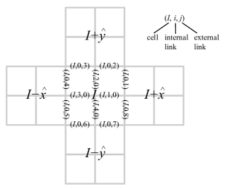
Figure 6: Our notation for the links.

Let $I$ denote a cell of four plaquettes. See Fig. 6. The four neighboring cells are called $I+\hat{x}$, $I-\hat{x}$, $I+\hat{y}$, and $I-\hat{y}$. Each cell has four internal links with spin-$\tfrac{1}{2}$ operators $\vec{\sigma}_{I,i,0}$, $i=1,\dotsc,4$. Also, each cell is surrounded by eight external links with spin-$\tfrac{1}{2}$ operators $\vec{\sigma}_{I,0,j}$, $j=1,\dotsc,8$. The ordering convention is explained in the figure.

Since external links that are on the boundary of a given cell are shared in common with one other neighboring cell, it will be useful to have a notation denoting an equivalent link from the perspective of the neighbor. If $(I,0,j)$ is a given link in a given cell, then the neighboring cell that shares that link will be denoted ${I^{[j]}}$, and the same link will, from this cell’s perspective, be called $[j]$. Explicitly,

$$(I,0,j) = ({I^{[j]}},0,[j])$$ (39)

$$(I,0,8) = (I+\hat{x},0,5)$$

$$(I,0,1) = (I+\hat{x},0,4)$$

$$(I,0,2) = (I+\hat{y},0,7)$$

$$(I,0,3) = (I+\hat{y},0,6)$$

$$(I,0,4) = (I-\hat{x},0,1)$$

$$(I,0,5) = (I-\hat{x},0,8)$$

$$(I,0,6) = (I-\hat{y},0,3)$$

$$(I,0,7) = (I-\hat{y},0,2).$$

Separate the Hamiltonian into an intracell part and intercell part,

$$H_{\sigma}=H_{\sigma}^{0}+V_{\sigma}.$$ (40)

The intracell part is a sum over all cells of the internal links, including both $\sigma^{x}$ and $\sigma^{z}$ operators, and the external links, but including only the $\sigma^{x}$ operators. Let

$$H_{\sigma}^{0}=\sum_{I}H_{I}^{0},$$ (41a)

where

$$H_{I}^{0}=-h\sum_{i=1}^{4}\sigma^{z}_{I,i,0}-J\sum_{i=1}^{4}\sigma^{x}_{I,i,0}\sigma^{x}_{I,i+1,0}\sigma^{x}_{I,0,2i-1}\sigma^{x}_{I,0,2i}.$$ (41b)

The intercell part is a collection of all transverse field operators acting on the external links of each cell,

$$V_{\sigma}=-h\sum_{I}\sum_{j=1}^{8}\sigma^{z}_{I,0,j}.$$ (42)

It is understood that all external links are to be summed over just once. As a shorthand we will write $\sum_{I,j}$.

It is important to notate eigenvalues of $\sigma^{x}$ operators on external links. For any $I$ and $j$, denote

$$\sigma^{x}_{I,0,j}|x_{I,j}\rangle_{I,0,j}=x_{I,j}|x_{I,j}\rangle_{I,0,j},\quad x_{I,j}=\pm 1.$$ (43)

Since $[H_{I}^{0},\sigma^{x}_{I,0,j}]=0$ for each $j$, each external link operator $\sigma^{x}_{I,0,j}$ may be replaced by its eigenvalue $x_{I,j}$. Thus, the eight bits $x_{I,j}$ behave as classical boundary conditions. For the cell Hamiltonian we may write $H_{I}^{0}(x_{I,1},\dotsc,x_{I,8})$.

Each cell, because it has four qubits and eight bits, would seem to have a $2^{4}$-dimensional Hilbert space for every classical configuration of its external links. However, gauge invariance reduces this large space of possibilities so that, ultimately, it matches the information encoded in the quantum Ising model with a block of four sites. First, $[H_{I}^{0},\prod_{i=1}^{4}\sigma^{z}_{I,i,0}]=0$ and we are interested only in the gauge-invariant sector $\prod_{i}\sigma^{z}_{I,i,0}=+1$. This halves the dimensionality from $2^{4}$ to $2^{3}$. And each eigenstate of $H_{I}^{0}$ has an eigenvalue that depends only on the sign of the gauge-invariant flux operator,

$$\Phi_{I}=\prod_{j=1}^{8}\sigma^{x}_{I,0,j}=\prod_{j=1}^{8}x_{I,j}.$$ (44)

That is, if we denote an eigenstate of $H_{I}^{0}$ by

$$|i_{I}(x_{I,1},\dotsc,x_{I,8})\rangle_{I},\quad i_{I}=0,\dotsc,7,$$ (45)

then its corresponding eigenvalue is some

$$\epsilon_{i_{I}}^{\text{c}}(\Phi_{I}).$$ (46)

The superscript “c” stands for “cell.” Thus, we are really dealing with a Hilbert space containing 16 eigenstates: 8 in the sector with $\Phi_{I}=+1$, and 8 in the sector with $\Phi_{I}=-1$. We reserve $i_{I}=0$ to indicate the lowest-energy state in either sector.

A.2 Cell spectrum

The explicit wavefunctions and energies for $H_{I}^{0}$ may be worked out by following the procedure in Ref. Fradkin and Raby, 1979. We use a basis for the internal links in which $\sigma^{z}_{I,i,0}$ is diagonal (i.e., $\sigma^{z}_{I,i,0}\!\uparrow_{i}\,=\,\uparrow_{i}$ and $\sigma^{z}_{I,i,0}\!\downarrow_{i}\,=-\!\downarrow_{i}$, and $\sigma^{x}_{I,i,0}\!\uparrow_{i}\,=\,\downarrow_{i}$ and $\sigma^{x}_{I,i,0}\!\downarrow_{i}\,=\,\uparrow_{i}$). The basis ordering is $\{\uparrow_{1}\uparrow_{2}\uparrow_{3}\uparrow_{4},\,\uparrow\downarrow\uparrow\downarrow,\,\downarrow\uparrow\downarrow\uparrow,\,\downarrow\downarrow\downarrow\downarrow,\,\uparrow\uparrow\downarrow\downarrow,\,\downarrow\downarrow\uparrow\uparrow,\,\uparrow\downarrow\downarrow\uparrow,\,\downarrow\uparrow\uparrow\downarrow\}$. Since all eigenstates are going to be expressed in this basis, the condition $\prod_{i}\sigma^{z}_{I,i,0}=+1$ is automatically satisfied. Define

$$A_{k}=x_{I,2k-1}x_{I,2k},\quad k=1,\dotsc,4.$$ (47)

Then

$$H_{I}^{0}=\begin{pmatrix}P&Q\\ Q^{T}&0\end{pmatrix},$$ (48a)

where

$$P = -4h\begin{pmatrix}1&&&\\ &0&&\\ &&0&\\ &&&-1\end{pmatrix},$$ (48b)

$$Q = -J\begin{pmatrix}A_{3}&A_{1}&A_{2}&A_{4}\\ A_{2}&A_{4}&A_{3}&A_{1}\\ A_{4}&A_{2}&A_{1}&A_{3}\\ A_{1}&A_{3}&A_{4}&A_{2}\\ \end{pmatrix}.$$ (48c)

Clearly, the wavefunctions are not functions of the eight $x_{I,j}$, but rather the four combinations $A_{k}$,

$$|i_{I}(x_{I,1},\dotsc,x_{I,8})\rangle_{I}=|i_{I}(A_{1},\dotsc,A_{4})\rangle_{I}.$$ (49)

We wish to solve the eigenvalue problem $H_{I}^{0}|i_{I}\rangle_{I}=\epsilon_{i_{I}}^{\text{c}}|i_{I}\rangle_{I}$ subject to additional constraints inherited from gauge invariance. In the full Hamiltonian $H$, gauge transformations are possible at each of the nine sites in cell $I$. However, because of the artificial nature of the blocking scheme the eight transformations around the cell perimeter no longer manifest as symmetries from the point of view of the cell Hamiltonian $H_{I}^{0}$. Instead, they manifest as the following identities (for the sake of brevity we only write parameters that are being affected in some way, e.g., by being negated):

$$H_{I}^{0}(x_{I,1},x_{I,2}) = H_{I}^{0}(-x_{I,1},-x_{I,2}),$$ (50a)

$$H_{I}^{0}(x_{I,3},x_{I,4}) = H_{I}^{0}(-x_{I,3},-x_{I,4}),$$ (50b)

$$H_{I}^{0}(x_{I,5},x_{I,6}) = H_{I}^{0}(-x_{I,5},-x_{I,6}),$$ (50c)

$$H_{I}^{0}(x_{I,7},x_{I,8}) = H_{I}^{0}(-x_{I,7},-x_{I,8}),$$ (50d)

and

$$\sigma^{z}_{I,1,0}H_{I}^{0}(x_{I,8},x_{I,1})\sigma^{z}_{I,1,0} = H_{I}^{0}(-x_{I,8},-x_{I,1}),\qquad$$ (51a)

$$\sigma^{z}_{I,2,0}H_{I}^{0}(x_{I,2},x_{I,3})\sigma^{z}_{I,2,0} = H_{I}^{0}(-x_{I,2},-x_{I,3}),$$ (51b)

$$\sigma^{z}_{I,3,0}H_{I}^{0}(x_{I,4},x_{I,5})\sigma^{z}_{I,3,0} = H_{I}^{0}(-x_{I,4},-x_{I,5}),$$ (51c)

$$\sigma^{z}_{I,4,0}H_{I}^{0}(x_{I,6},x_{I,7})\sigma^{z}_{I,4,0} = H_{I}^{0}(-x_{I,6},-x_{I,7}).$$ (51d)

Eqs. (50) correspond to the four corners of the cell, while Eqs. (51) correspond to the midpoints of each side. The former are trivially satisfied if we express the wavefunctions in terms of the $A_{k}$. However, the latter are nontrivial and require that

$$\sigma^{z}_{I,1,0}|i_{I}(A_{4},A_{1})\rangle_{I} = |i_{I}(-A_{4},-A_{1})\rangle_{I},$$ (52a)

$$\sigma^{z}_{I,2,0}|i_{I}(A_{1},A_{2})\rangle_{I} = |i_{I}(-A_{1},-A_{2})\rangle_{I},$$ (52b)

$$\sigma^{z}_{I,3,0}|i_{I}(A_{2},A_{3})\rangle_{I} = |i_{I}(-A_{2},-A_{3})\rangle_{I},$$ (52c)

$$\sigma^{z}_{I,4,0}|i_{I}(A_{3},A_{4})\rangle_{I} = |i_{I}(-A_{3},-A_{4})\rangle_{I}.$$ (52d)

Note that, in our chosen basis,

$$\sigma^{z}_{I,1,0} = \mathrm{diag}(+,+,-,-,+,-,+,-),$$ (53a)

$$\sigma^{z}_{I,2,0} = \mathrm{diag}(+,-,+,-,+,-,-,+),$$ (53b)

$$\sigma^{z}_{I,3,0} = \mathrm{diag}(+,+,-,-,-,+,-,+),$$ (53c)

$$\sigma^{z}_{I,4,0} = \mathrm{diag}(+,-,+,-,-,+,+,-).$$ (53d)

A.2.1 $\Phi_{I}=+$ sector

Cell energies arranged in increasing order are

$$\epsilon_{0}^{\text{c}}(+) = -2^{3/2}[h^{2}+J^{2}+(h^{4}+J^{4})^{1/2}]^{1/2},\quad$$ (54a)

$$\epsilon_{1}^{\text{c}}(+) = -2^{3/2}[h^{2}+J^{2}-(h^{4}+J^{4})^{1/2}]^{1/2},$$ (54b)

$$\epsilon_{2}^{\text{c}}(+) = 0,$$ (54c)

$$\epsilon_{3}^{\text{c}}(+) = 0,$$ (54d)

$$\epsilon_{4}^{\text{c}}(+) = 0,$$ (54e)

$$\epsilon_{5}^{\text{c}}(+) = 0,$$ (54f)

$$\epsilon_{6}^{\text{c}}(+) = 2^{3/2}[h^{2}+J^{2}-(h^{4}+J^{4})^{1/2}]^{1/2},$$ (54g)

$$\epsilon_{7}^{\text{c}}(+) = 2^{3/2}[h^{2}+J^{2}+(h^{4}+J^{4})^{1/2}]^{1/2}.$$ (54h)

There is no level crossing. For $i_{I}=0,1,6,7$, let $E=\epsilon_{i_{I}}^{\text{c}}(+)$ for brevity. The unnormalized wavefunction is

$$|0,1,6,7\rangle_{I}=\begin{pmatrix}4J(E+4h)^{-1}\\ \Gamma(E-4h)A_{2}A_{3}\\ \Gamma(E-4h)A_{3}A_{4}\\ \Gamma EA_{1}A_{3}\\ -A_{3}\\ -A_{1}\\ -A_{2}\\ -A_{4}\end{pmatrix},$$ (55a)

where

$$\Gamma=\frac{E^{2}+4hE-4J^{2}}{J(E+4h)(3E-8h)}.$$ (55b)

For $$i_{I}=2,3,4,5$$, the normalized wavefunctions are

$$|2\rangle_{I}=\frac{1}{\sqrt{2}}\begin{pmatrix}0\\ A_{1}A_{4}\\ -A_{3}A_{4}\\ 0\\ 0\\ 0\\ 0\\ 0\end{pmatrix},\quad|3\rangle_{I}=\frac{1}{\sqrt{2}}\begin{pmatrix}0\\ 0\\ 0\\ 0\\ A_{3}\\ 0\\ 0\\ -A_{4}\end{pmatrix},$$

$$|4\rangle_{I}=\frac{1}{\sqrt{2}}\begin{pmatrix}0\\ 0\\ 0\\ 0\\ 0\\ A_{1}\\ -A_{2}\\ 0\end{pmatrix},\quad|5\rangle_{I}=\frac{1}{2}\begin{pmatrix}0\\ 0\\ 0\\ 0\\ A_{3}\\ -A_{1}\\ -A_{2}\\ A_{4}\end{pmatrix}.$$ (55c)

It is important to note that $\{|2\rangle_{I},|3\rangle_{I},|4\rangle_{I},|5\rangle_{I}\}$ form an orthonormal basis in the zero-energy subspace. Obtaining these particular wavefunctions required judicious use of identities like $A_{k}=1/A_{k}$, and $A_{1}=A_{2}A_{3}A_{4}$, $A_{1}A_{2}=A_{3}A_{4}$, etc. which follows from the fact that $A_{1}A_{2}A_{3}A_{4}=1$.

A.2.2 $\Phi_{I}=-$ sector

Cell energies arranged in increasing order are, for $h>0$,

$$\epsilon_{0}^{\text{c}}(-) = -2(h^{2}+J^{2})^{1/2}-2h$$ (56a)

$$\epsilon_{1}^{\text{c}}(-) = -2J$$ (56b)

$$\epsilon_{2}^{\text{c}}(-) = -2J$$ (56c)

$$\epsilon_{3}^{\text{c}}(-) = -2(h^{2}+J^{2})^{1/2}+2h$$ (56d)

$$\epsilon_{4}^{\text{c}}(-) = 2(h^{2}+J^{2})^{1/2}-2h$$ (56e)

$$\epsilon_{5}^{\text{c}}(-) = 2J$$ (56f)

$$\epsilon_{6}^{\text{c}}(-) = 2J$$ (56g)

$$\epsilon_{7}^{\text{c}}(-) = 2(h^{2}+J^{2})^{1/2}+2h.$$ (56h)

For $i_{I}=0,4,3,7$, let $E=\epsilon^{\text{c}}_{i_{I}}(-)$ for brevity. The normalized wavefunctions are

$$|0,4\rangle_{I}=\frac{1}{\sqrt{4+E^{2}/J^{2}}}\begin{pmatrix}-EJ^{-1}\\ 0\\ 0\\ 0\\ A_{3}\\ A_{1}\\ A_{2}\\ A_{4}\end{pmatrix},$$ (57)

$$|3,7\rangle_{I}=\frac{1}{\sqrt{4+E^{2}/J^{2}}}\begin{pmatrix}0\\ 0\\ 0\\ -EJ^{-1}A_{1}A_{3}\\ A_{3}\\ A_{1}\\ -A_{2}\\ -A_{4}\end{pmatrix},$$

$$|1\rangle_{I}=\frac{1}{\sqrt{8}}\begin{pmatrix}0\\ 2A_{2}A_{3}\\ 0\\ 0\\ A_{3}\\ -A_{1}\\ A_{2}\\ -A_{4}\end{pmatrix},\quad|5\rangle_{I}=\frac{1}{\sqrt{8}}\begin{pmatrix}0\\ -2A_{2}A_{3}\\ 0\\ 0\\ A_{3}\\ -A_{1}\\ A_{2}\\ -A_{4}\end{pmatrix},$$

$$|2\rangle_{I}=\frac{1}{\sqrt{8}}\begin{pmatrix}0\\ 0\\ 2A_{1}A_{2}\\ 0\\ -A_{3}\\ A_{1}\\ A_{2}\\ -A_{4}\end{pmatrix},\quad|6\rangle_{I}=\frac{1}{\sqrt{8}}\begin{pmatrix}0\\ 0\\ -2A_{1}A_{2}\\ 0\\ -A_{3}\\ A_{1}\\ A_{2}\\ -A_{4}\end{pmatrix}.$$

A.3 Lattice eigenstates as products of cell and external link eigenstates

For any given configuration on the external links, the lowest energy eigenstate of $H_{\sigma}^{0}$ is obtained from a product over all cells with $i_{I}=0$,

$$|i\rangle=\prod_{I,j}|0(x_{I,1},\dotsc,x_{I,8})\rangle_{I}|x_{I,j}\rangle_{I,0,j},$$ (58)

where it is understood that each external link contributes just once. The $H_{\sigma}^{0}$-eigenvalue is

$$\epsilon_{i}=\sum_{I}\epsilon_{0}^{\text{c}}(\Phi_{I}).$$ (59)

When summing over all possible $|i\rangle$ we shall use the shorthand

$$\sum_{i}=\prod_{I,j}\sum_{x_{I,j}=\pm 1}.$$ (60)

Corresponding to each state $|i\rangle$ in the Hilbert space of the original lattice Hamiltonian is a state $|\mu_{i}\rangle$ belonging to the smaller Hilbert space of the renormalized Hamiltonian. Quite simply, it is everything in $|i\rangle$ but the wavefunction of the internal links.

$$|\mu_{i}\rangle=\prod_{I,j}|x_{I,j}\rangle_{I,0,j}.$$ (61)

It is in this sense that the internal links have been “decimated.” On the thinner lattice of external links $\{|x_{I,j}\rangle_{I,0,j}\}$ we define new Pauli operators

$$\mathrm{1\!\!1}_{I,j} = (|+\rangle\langle+|+|-\rangle\langle-|)_{I,0,j},$$ (62a)

$$\mu^{x}_{I,j} = (|+\rangle\langle+|-|-\rangle\langle-|)_{I,0,j},$$ (62b)

$$\mu^{z}_{I,j} = (|+\rangle\langle-|+|-\rangle\langle+|)_{I,0,j}.$$ (62c)

Since $\{|i\rangle\}$ is merely a small subset of the energy basis of $H_{\sigma}^{0}$, the remaining higher-energy lattice eigenstates are constructed from cells with any value of $i_{I}$,

$$|\alpha\rangle=\prod_{I,j}|i_{I}(x_{I,1},\dotsc,x_{I,8})\rangle_{I}|x_{I,j}\rangle_{I,0,j},\quad i_{I}=0,\dotsc,7,$$ (63)

with the caveat that at least one $i_{I}>0$. Its $H_{\sigma}^{0}$-eigenvalue is

$$\epsilon_{\alpha}=\sum_{I}\epsilon_{i_{I}}^{\text{c}}(\Phi_{I}).$$ (64)

When summing over all possible $|\alpha\rangle$ we shall use the shorthand

$$\sum_{\alpha}=\prod_{I,j}\sum_{i_{I}=0}^{7}\biggr{|}_{\text{some $i_{I}\neq 0$}}\sum_{x_{I,j}=\pm 1}.$$ (65)

A.4 Hirsch–Mazenko perturbation expansion

To second order in the intercell coupling,

$$H^{\text{ren}}_{\mu} = H_{\mu}^{(0)}+H_{\mu}^{(1)}+H_{\mu}^{(2)}+\dotsb,$$ (66a)

$$H^{(0)}_{\mu} = \sum_{i}\epsilon_{i}|\mu_{i}\rangle\langle\mu_{i}|,$$ (66b)

$$H^{(1)}_{\mu} = \sum_{i,i^{\prime}}\langle i^{\prime}|V_{\sigma}|i\rangle|\mu_{i}\rangle\langle\mu_{i^{\prime}}|,$$ (66c)

$$H^{(2)}_{\mu} = \tfrac{1}{2}\sum_{i,i^{\prime}}\sum_{\alpha}\langle i^{\prime}|V_{\sigma}|\alpha\rangle\langle\alpha|V_{\sigma}|i\rangle$$ (66d)

$$\times\Bigl{(}\frac{1}{\epsilon_{i}-\epsilon_{\alpha}}+\frac{1}{\epsilon_{i^{\prime}}-\epsilon_{\alpha}}\Bigr{)}|\mu_{i}\rangle\langle\mu_{i^{\prime}}|.$$

Refer to Ref. Hirsch and Mazenko, 1979 for a derivation of these expressions. They have been written in a simplified form following Eq. (3) of Ref. Hirsch, 1979.

When there is no chance of confusion, we will abbreviate the state $|x_{I,j}\rangle_{I,0,j}$ as $|x_{I,j}\rangle$.

A.4.1 Computation of $H_{\mu}^{(0)}$

Consider Eq. (66b),

$$H^{(0)}_{\mu}=\Bigl{(}\prod_{I,j}\sum_{x_{I,j}}\Bigr{)}\Bigl{(}\sum_{I}\epsilon_{0}^{\text{c}}(\Phi_{I})\Bigr{)}\prod_{I,j}|x_{I,j}\rangle\langle x_{I,j}|.$$ (67a)

Bring the sum over cells $$I \Phi_{I} I b_{1},\dotsc,b_{8}$$ out so that only the links belonging to a given will be non-identity operators. Call the eight links of cell , . Then

$$H^{(0)}_{\mu} = \sum_{I}\sum_{x_{b_{1}}}\dotsb\sum_{x_{b_{8}}}\epsilon_{0}^{\text{c}}(x_{b_{1}}\dotsb x_{b_{8}})$$ (67c)

$$\times|x_{b_{1}}\rangle\langle x_{b_{1}}|\dotsb|x_{b_{8}}\rangle\langle x_{b_{8}}|$$

$$= \sum_{I}\Big{(}\frac{\epsilon_{0}^{\text{c}}(+)+\epsilon_{0}^{\text{c}}(-)}{2}\mathrm{1\!\!1}_{b_{1}}\dotsb\mathrm{1\!\!1}_{b_{8}}$$

$$-\frac{\epsilon_{0}^{\text{c}}(-)-\epsilon_{0}^{\text{c}}(+)}{2}\mu^{x}_{b_{1}}\dotsb\mu^{x}_{b_{8}}\Bigr{)}.$$

A.4.2 Computation of $H_{\mu}^{(1)}$

Consider Eq. (66c),

$$H_{\mu}^{(1)}=\Bigl{(}\prod_{I,j}\sum_{x_{I,j}}\Bigr{)}\Bigl{(}\prod_{I,j}\sum_{x^{\prime}_{I,j}}\Bigr{)}\prod_{I,j}\langle 0(\{x^{\prime}_{I,j}\})|_{I}\langle x^{\prime}_{I,j}|\cdot-h\sum_{I,j}\sigma^{z}_{I,0,j}\cdot\prod_{I,j}|0(\{x_{I,j}\})\rangle_{I}|x_{I,j}\rangle\cdot\prod_{I,j}|x_{I,j}\rangle\langle x^{\prime}_{I,j}|.$$ (68a)

By an abuse of notation, each instance of “$$\prod_{I,j} \cdot ) \sum_{I,j} (I,0,j) \langle x^{\prime}_{I,j}|\sigma^{z}_{I,0,j}|x_{I,j}\rangle=\delta_{x^{\prime}_{I,j},-x_{I,j}} x^{\prime}_{I,j} x_{I,j} {\tilde{I}} (I,0,j) \langle 0|0\rangle_{\tilde{I}}=1 I {I^{[j]}}$$” serves to remind us that there are as many copies of the expression immediately to the right of this symbol but left of “” or “” as external links in the lattice. Pull out . For a single external link at , we get the constraint . At all other external links the eigenvalues and are equal. Therefore, all cells not containing link on their border yield . Only cells and share this link. So

$$H_{\mu}^{(1)} = -h\sum_{I,j}\sum_{x_{I,j}}\sum_{x_{b_{1}}}\dotsb\sum_{x_{b_{13}}}$$ (68b)

$$\times\langle 0(-x_{I,j})|0(x_{I,j})\rangle_{I}\langle 0(-x_{{I^{[j]}},[j]})|0(x_{{I^{[j]}},[j]})\rangle_{I^{[j]}}$$

$$\times|x_{I,j}\rangle\langle-x_{I,j}|\prod_{b=1}^{13}|x_{b}\rangle\langle x_{b}|,$$

where $$b_{1},\dotsc,b_{13} I {I^{[j]}} (I,0,j)=({I^{[j]}},0,[j]) \langle 0(-x_{I,j})|0(x_{I,j})\rangle_{I} j x_{I,j} I x_{b_{1}},\dotsc,x_{b_{7}} j x_{I,j},\,x_{b_{1}},\dotsc,x_{b_{7}} j=1 x_{I,j}=x_{b_{1}}=\dotsb=x_{b_{7}}=+ \Phi_{I}=+ \Phi_{I}=-$$ denote all links in cells and besides . Consider the matrix element . Besides the choice of and the value of it could also depend on the seven additional external link eigenvalues forming the rest of the boundary of . Let us call them (we have suppressed writing these as they are not negated in the inner product). However, it turns out that this matrix element is completely independent of boundary conditions. That is, the matrix element evaluates to the same quantity for any choice of and the values . For convenience let us select , . So the matrix element is an inner product between the two lowest energy states from the and sectors, respectively. For future convenience define these states to be (with specific boundary conditions)

$$|0_{+}\rangle_{I} = |0(A_{1}=+,A_{2}=+,A_{3}=+,A_{4}=+)\rangle_{I},\qquad\qquad$$ (68c)

$$|0_{-}\rangle_{I} = |0(A_{1}=+,A_{2}=-,A_{3}=+,A_{4}=+)\rangle_{I}.$$ (68d)

Although it seems peculiar to make $$A_{2} A_{1}$$ negative in Eq. (68d) rather than, say, , in hindsight this choice allows us to write all matrix elements using only these two states. We will return to this point later. Thus,

$$H_{\mu}^{(1)}=-2h|\langle 0_{-}|0_{+}\rangle_{I}|^{2}\sum_{I,j}\mu^{z}_{I,j}.$$ (68e)

The factor of 2 arises from the fact that each side of a cell contributes two links.

A.4.3 Computation of $H_{\mu}^{(2)}$

When fully written out Eq. (66d) is

$$H_{\mu}^{(2)} = \tfrac{1}{2}\Bigl{(}\prod_{I,j}\sum_{x^{\prime\prime}_{I,j}}\Bigr{)}\Bigl{(}\prod_{I,j}\sum_{x^{\prime}_{I,j}}\Bigr{)}\Bigl{(}\prod_{I,j}\sum_{i_{I}=0}^{7}\Bigr{|}_{\text{some $i_{I}\neq 0$}}\sum_{x_{I,j}}\Bigr{)}$$ (69)

$$\prod_{I,j}\langle 0(\{x^{\prime}_{I,j}\})|_{I}\langle x^{\prime}_{I,j}|\cdot-h\sum_{I,j}\sigma^{z}_{I,0,j}\cdot\prod_{I,j}|i_{I}(\{x_{I,j}\})\rangle_{I}|x_{I,j}\rangle$$

$$\times\prod_{I,j}\langle i_{I}(\{x_{I,j}\})|_{I}\langle x_{I,j}|\cdot-h\sum_{I^{\prime},j^{\prime}}\sigma^{z}_{I^{\prime},0,j^{\prime}}\cdot\prod_{I,j}|0(\{x^{\prime\prime}_{I,j}\})\rangle_{I}|x^{\prime\prime}_{I,j}\rangle$$

$$\times\Bigl{(}\frac{1}{\sum_{I}[\epsilon_{0}^{\text{c}}(\Phi^{\prime\prime}_{I})-\epsilon_{i_{I}}^{\text{c}}(\Phi_{I})]}+\frac{1}{\sum_{I}[\epsilon_{0}^{\text{c}}(\Phi^{\prime}_{I})-\epsilon_{i_{I}}^{\text{c}}(\Phi_{I})]}\Bigr{)}\cdot\prod_{I,j}|x^{\prime\prime}_{I,j}\rangle\langle x^{\prime}_{I,j}|,$$

where $\Phi_{I}=\prod_{j=1}^{8}x_{I,j}$, $\Phi^{\prime}_{I}=\prod_{j=1}^{8}x^{\prime}_{I,j}$, and $\Phi^{\prime\prime}_{I}=\prod_{j=1}^{8}x^{\prime\prime}_{I,j}$, Pull out $\sum_{I,j}$ and $\sum_{I^{\prime},j^{\prime}}$; eventually, we will want to keep just one of these sums unevaluated. It is possible to completely evaluate $\prod_{I,j}\sum_{x^{\prime\prime}_{I,j}}$ and $\prod_{I,j}\sum_{x^{\prime}_{I,j}}$ by collapsing Kronecker deltas for external links. For links $b\neq(I,0,j)$, $x^{\prime}_{b}=x_{b}$, but for the the special link $b=(I,0,j)$, $x^{\prime}_{b}=-x_{b}$. Similarly, for links $b\neq(I^{\prime},0,j^{\prime})$, $x^{\prime\prime}_{b}=x_{b}$, but for the special link $b=(I^{\prime},0,j^{\prime})$, $x^{\prime\prime}_{b}=-x_{b}$.

Consequently, two kinds of inner product between cell wavefunctions may result. If a given cell ${\tilde{I}}$ does not contain the special link $(I,0,j)$, then orthonormality requires that $i_{\tilde{I}}=0$. Likewise, if a given cell ${\overline{I}}$ does not contain the special link $(I^{\prime},0,j^{\prime})$, then $i_{\overline{I}}=0$. This results in a drastic simplification of the energy denominators. For convenience define

$$R_{i_{I},i_{I^{[j]}}}(\Phi_{I},\Phi_{I^{[j]}}) = \Bigl{[}\epsilon_{0}^{\text{c}}(-\Phi_{I})+\epsilon_{0}^{\text{c}}(-\Phi_{I^{[j]}})$$ (70)

$$-\epsilon_{i_{I}}^{\text{c}}(\Phi_{I})-\epsilon_{i_{I^{[j]}}}^{\text{c}}(\Phi_{I^{[j]}})\Bigr{]}^{-1}.\qquad$$

However, if a cell does have one of these special links sitting on its boundary—there will be two in the case of $(I,0,j)$: $I$ and ${I^{[j]}}$, and two in the case of $(I^{\prime},0,j^{\prime})$: $I^{\prime}$ and ${{I^{\prime}}^{[j^{\prime}]}}$—then an extra minus sign appears in one of the eight parameters in one of the two wavefunctions participating in the inner product. It shall be convenient to define

$$\zeta_{i_{I}}^{j}(\Phi_{I})=\langle 0(-x_{I,j},\{x_{I,k}\}_{k\neq j})|i_{I}(x_{I,j},\{x_{I,k}\}_{k\neq j})\rangle_{I}.$$ (71)

Eq. (71) has an important property: although it depends on the choice of $i_{I}$ and $j$, it does not depend on the precise choice of the $x_{I,j}$ except for the overall sign of $\Phi_{I}$.

At this step,

$$H_{\mu}^{(2)} = \frac{h^{2}}{2}\sum_{I,j}\sum_{I^{\prime},j^{\prime}}\Bigl{(}\prod_{I,j}\sum_{i_{I}}\Bigr{|}_{\text{some $i_{I}\neq 0$}}\sum_{x_{I,j}}\Bigr{)}\prod_{{\tilde{I}}\not\ni(I,0,j)}\delta_{0,i_{\tilde{I}}}\prod_{{\overline{I}}\not\ni(I^{\prime},0,j^{\prime})}\delta_{0,i_{\overline{I}}}$$ (74)

$$\times\zeta_{i_{I}}^{j}(\Phi_{I})\zeta_{i_{I^{[j]}}}^{[j]}(\Phi_{I^{[j]}})\zeta^{j^{\prime}}_{i_{I^{\prime}}}(\Phi_{I^{\prime}})\zeta^{[j^{\prime}]}_{i_{{I^{\prime}}^{[j^{\prime}]}}}(\Phi_{{I^{\prime}}^{[j^{\prime}]}})\Bigl{(}R_{i_{I},i_{I^{[j]}}}(\Phi_{I},\Phi_{I^{[j]}})+R_{i_{I^{\prime}},i_{{I^{\prime}}^{[j^{\prime}]}}}(\Phi_{I^{\prime}},\Phi_{{I^{\prime}}^{[j^{\prime}]}})\Bigr{)}$$

$$\times\prod_{b\neq(I,0,j),\,(I^{\prime},0,j^{\prime})}(|x_{b}\rangle\langle x_{b}|)_{b}\times\Biggl{\{}\begin{array}[]{ll}(|-x_{I,j}\rangle\langle-x_{I,j}|)_{I,0,j}&(I^{\prime},0,j^{\prime})=(I,0,j)\\ (|-x_{I^{\prime},j^{\prime}}\rangle\langle x_{I^{\prime},j^{\prime}}|)_{I^{\prime},0,j^{\prime}}\;(|x_{I,j}\rangle\langle-x_{I,j}|)_{I,0,j}&(I^{\prime},0,j^{\prime})\neq(I,0,j)\\ \end{array}.\quad$$

If we use up the remaining Kronecker deltas over cells, then the decimation of internal links will be complete. However, there is not necessarily one Kronecker delta per cell since the number of such constraints that get enforced depends on the relative location of link $(I^{\prime},0,j^{\prime})$ to link $(I,0,j)$. For imagine that $(I,0,j)$ is fixed. If $(I^{\prime},0,j^{\prime})$ is located at…

1. Any of the two links on the shared boundary of $I$ and ${I^{[j]}}$, then $I^{\prime}$ and ${{I^{\prime}}^{[j^{\prime}]}}$ coincide with $I$ and ${I^{[j]}}$ precisely. Therefore, Kronecker deltas will not exist for these two cells. And $\sum_{i_{I}}$ and $\sum_{i_{I^{[j]}}}$ will be left undone;

2. Any of the twelve links on the outer perimeter of the union of $I$ and ${I^{[j]}}$, then either $I^{\prime}$ or ${{I^{\prime}}^{[j^{\prime}]}}$ will coincide with one of $I$ and ${I^{[j]}}$. Therefore, a Kronecker delta will not exist for that doubly-covered cell. Say this is $I$. Then $\sum_{i_{I}}$ will be left undone;

3. Any other link on the lattice, then $I^{\prime}$ and ${{I^{\prime}}^{[j^{\prime}]}}$ will not overlap $I$ and ${I^{[j]}}$ at all. Therefore, a Kronecker delta exists for all cells.

In terms of these three general cases, let us write

$$H^{(2)}_{\mu}=\frac{h^{2}}{2}\sum_{I,j}(\text{Case 1}+\text{Case 2}+\text{Case 3}).$$ (75)

Case 3

If every cell is constrained to be in its ground state, then there cannot be an intermediate excited state (i.e., $\sum_{i_{I}}|_{\text{some $i_{I}\neq 0$}}$ is null). Thus,

$$\text{Case 3}=0.$$ (76)

Case 1

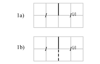
Figure 7: Subcases 1a and 1b. Links $(I,0,j)$ and $(I^{\prime},0,j^{\prime})$ are represented by the bold and dashed links, respectively. In Subcase 1a they are the same link.

There are two subcases: (a) $(I^{\prime},0,j^{\prime})=(I,0,j)$, and (b) $(I^{\prime},0,j^{\prime})\neq(I,0,j)$, such that

$$\text{Case 1}=\text{Subcase 1a}+\text{Subcase 1b}.$$ (77)

See Fig. 7. For all external links that are not on the two neighboring cells that share the links $(I,0,j)$ and $(I^{\prime},0,j^{\prime})$, we obtain the identity operator since $\sum_{x_{b}}(|x_{b}\rangle\langle x_{b}|)_{b}=\mathrm{1\!\!1}_{b}$. There are fourteen link sums left to do.

Consider Subcase 1a. Define

$$C^{j,i_{I},i_{I^{[j]}}}(\Phi_{I},\Phi_{I^{[j]}}) = \zeta_{i_{I}}^{j}(\Phi_{I})^{2}\zeta_{i_{I^{[j]}}}^{[j]}(\Phi_{I^{[j]}})^{2}$$ (78)

$$\times 2R_{i_{I},i_{I^{[j]}}}(\Phi_{I},\Phi_{I^{[j]}}).\quad$$

This is, essentially, the second line in Eq. (74). Summing over the fourteen external links and using the identity $\mu^{x}_{b}\mu^{x}_{b}=\mathrm{1\!\!1}_{b}$ gives

Subcase 1a $$= \Biggl{(}\sum_{i_{I^{[j]}}=1}^{7}\Bigr{|}_{i_{I}=0}+\sum_{i_{I}=1}^{7}\Bigr{|}_{i_{I^{[j]}}=0}+\sum_{i_{I}=1}^{7}\sum_{i_{I^{[j]}}=1}^{7}\Biggr{)}$$ (79)

$$\Biggl{[}S_{++++}^{j,i_{I},i_{I^{[j]}}}\prod_{b\in I}\mathrm{1\!\!1}_{b}\cdot\prod_{b\in{I^{[j]}}}\mathrm{1\!\!1}_{b}$$

$$+S_{+--+}^{j,i_{I},i_{I^{[j]}}}\prod_{b\in I}\mu_{b}^{x}\cdot\prod_{b\in{I^{[j]}}}\mu_{b}^{x}$$

$$-S_{++--}^{j,i_{I},i_{I^{[j]}}}\prod_{b\in I}\mu_{b}^{x}\cdot\prod_{b\in{I^{[j]}}}\mathrm{1\!\!1}_{b}$$

$$-S_{+-+-}^{j,i_{I},i_{I^{[j]}}}\prod_{b\in I}\mathrm{1\!\!1}_{b}\cdot\prod_{b\in{I^{[j]}}}\mu_{b}^{x}\Biggr{]},$$

where

$$S_{\sigma_{1}\sigma_{2}\sigma_{3}\sigma_{4}}^{j,i_{I},i_{I^{[j]}}} = \frac{1}{4}\Bigl{[}\sigma_{1}C^{j,i_{I},i_{I^{[j]}}}(+,+)$$ (80)

$$+\sigma_{2}C^{j,i_{I},i_{I^{[j]}}}(+,-)$$

$$+\sigma_{3}C^{j,i_{I},i_{I^{[j]}}}(-,+)$$

$$+\sigma_{4}C^{j,i_{I},i_{I^{[j]}}}(-,-)\Bigr{]}.$$

Further consolidation is achieved by defining

$$S_{1} = \sum_{i_{I^{[j]}}=1}^{7}S_{++++}^{j,0,i_{I^{[j]}}}+\sum_{i_{I}=1}^{7}S_{++++}^{j,i_{I},0}$$ (81a)

$$+\sum_{i_{I}=1}^{7}\sum_{i_{I^{[j]}}=1}^{7}S_{++++}^{j,i_{I},i_{I^{[j]}}},$$

$$S_{2} = \sum_{i_{I^{[j]}}=1}^{7}S_{+--+}^{j,0,i_{I^{[j]}}}+\sum_{i_{I}=1}^{7}S_{+--+}^{j,i_{I},0}$$ (81b)

$$+\sum_{i_{I}=1}^{7}\sum_{i_{I^{[j]}}=1}^{7}S_{+--+}^{j,i_{I},i_{I^{[j]}}},$$

$$S_{3} = \sum_{i_{I^{[j]}}=1}^{7}S_{++--}^{j,0,i_{I^{[j]}}}+\sum_{i_{I}=1}^{7}S_{++--}^{j,i_{I},0}$$ (81d)

$$+\sum_{i_{I}=1}^{7}\sum_{i_{I^{[j]}}=1}^{7}S_{++--}^{j,i_{I},i_{I^{[j]}}}$$

$$= \sum_{i_{I^{[j]}}=1}^{7}S_{+-+-}^{j,0,i_{I^{[j]}}}+\sum_{i_{I}=1}^{7}S_{+-+-}^{j,i_{I},0}$$

$$+\sum_{i_{I}=1}^{7}\sum_{i_{I^{[j]}}=1}^{7}S_{+-+-}^{j,i_{I},i_{I^{[j]}}}.$$

We have checked that expressions (81d) and (81d) are equivalent. Furthermore, none of the expressions for $S_{1}$, $S_{2}$, and $S_{3}$ depend on the choice of parameter $j$. This is expected since the lattice remains unchanged by $90^{\circ}$ rotations, or reflections about a horizontal or vertical line. Letting $\Phi_{I}=\prod_{b\in I}\mu_{b}^{x}$, we get

Subcase 1a $$= S_{1}+S_{2}\Phi_{I}\Phi_{I^{[j]}}$$ (82)

$$-S_{3}(\Phi_{I}+\Phi_{I^{[j]}}).$$

Next consider Subcase 1b. Define

$$D^{j,i_{I},i_{I^{[j]}}}(\Phi_{I},\Phi_{I^{[j]}}) = \zeta_{i_{I}}^{j}(\Phi_{I})\zeta_{i_{I^{[j]}}}^{[j]}(\Phi_{I^{[j]}})\zeta_{i_{I}}^{j^{\prime}}(\Phi_{I})\zeta_{i_{I^{[j]}}}^{[j^{\prime}]}(\Phi_{I^{[j]}})$$ (83)

$$\times 2R_{i_{I},i_{I^{[j]}}}(\Phi_{I},\Phi_{I^{[j]}}).$$

Summing over the fourteen external links and using the identity $(|-\rangle\langle+|-|+\rangle\langle-|)_{b}=\mathrm{i}\mu^{y}_{b}=\mu^{z}_{b}\mu^{x}_{b}$ gives

Subcase 1b $$= \Biggl{(}\sum_{i_{I^{[j]}}=1}^{7}\Bigr{|}_{i_{I}=0}+\sum_{i_{I}=1}^{7}\Bigr{|}_{i_{I^{[j]}}=0}+\sum_{i_{I}=1}^{7}\sum_{i_{I^{[j]}}=1}^{7}\Biggr{)}$$ (84)

$$\mu_{I,j}^{z}\mu_{I,j^{\prime}}^{z}\Biggl{[}T_{++++}^{j,i_{I},i_{I^{[j]}}}\prod_{b\in I}\mathrm{1\!\!1}_{b}\cdot\prod_{b\in{I^{[j]}}}\mathrm{1\!\!1}_{b}$$

$$+T_{+--+}^{j,i_{I},i_{I^{[j]}}}\prod_{b\in I}\mu_{b}^{x}\cdot\prod_{b\in{I^{[j]}}}\mu_{b}^{x}$$

$$-T_{++--}^{j,i_{I},i_{I^{[j]}}}\prod_{b\in I}\mu_{b}^{x}\cdot\prod_{b\in{I^{[j]}}}\mathrm{1\!\!1}_{b}$$

$$-T_{+-+-}^{j,i_{I},i_{I^{[j]}}}\prod_{b\in I}\mathrm{1\!\!1}_{b}\cdot\prod_{b\in{I^{[j]}}}\mu_{b}^{x}\Biggr{]},$$

where

$$T_{\sigma_{1}\sigma_{2}\sigma_{3}\sigma_{4}}^{j,i_{I},i_{I^{[j]}}} = \frac{1}{4}\Bigl{[}\sigma_{1}D^{j,i_{I},i_{I^{[j]}}}(+,+)$$ (85)

$$+\sigma_{2}D^{j,i_{I},i_{I^{[j]}}}(+,-)$$

$$+\sigma_{3}D^{j,i_{I},i_{I^{[j]}}}(-,+)$$

$$+\sigma_{4}D^{j,i_{I},i_{I^{[j]}}}(-,-)\Bigr{]}.$$

Once again, further consolidation is achieved by defining

$$T_{1} = \sum_{i_{I^{[j]}}=1}^{7}T_{++++}^{j,0,i_{I^{[j]}}}+\sum_{i_{I}=1}^{7}T_{++++}^{j,i_{I},0}$$ (86a)

$$+\sum_{i_{I}=1}^{7}\sum_{i_{I^{[j]}}=1}^{7}T_{++++}^{j,i_{I},i_{I^{[j]}}},$$

$$T_{2} = \sum_{i_{I^{[j]}}=1}^{7}T_{+--+}^{j,0,i_{I^{[j]}}}+\sum_{i_{I}=1}^{7}T_{+--+}^{j,i_{I},0}$$ (86b)

$$+\sum_{i_{I}=1}^{7}\sum_{i_{I^{[j]}}=1}^{7}T_{+--+}^{j,i_{I},i_{I^{[j]}}},$$

$$T_{3} = \sum_{i_{I^{[j]}}=1}^{7}T_{++--}^{j,0,i_{I^{[j]}}}+\sum_{i_{I}=1}^{7}T_{++--}^{j,i_{I},0}$$ (86d)

$$+\sum_{i_{I}=1}^{7}\sum_{i_{I^{[j]}}=1}^{7}T_{++--}^{j,i_{I},i_{I^{[j]}}}$$

$$= \sum_{i_{I^{[j]}}=1}^{7}T_{+-+-}^{j,0,i_{I^{[j]}}}+\sum_{i_{I}=1}^{7}T_{+-+-}^{j,i_{I},0}$$

$$+\sum_{i_{I}=1}^{7}\sum_{i_{I^{[j]}}=1}^{7}T_{+-+-}^{j,i_{I},i_{I^{[j]}}}.$$

We have checked that expressions (86d) and (86d) are equivalent, and that none of the expressions for $T_{1}$, $T_{2}$, and $T_{3}$ depend on the choice of parameter $j$. Thus,

Subcase 1b $$= \mu^{z}_{I,j}\mu^{z}_{I,j^{\prime}}[T_{1}+T_{2}\Phi_{I}\Phi_{I^{[j]}}$$ (87)

$$-T_{3}(\Phi_{I}+\Phi_{I^{[j]}})].$$

Case 2

There are twelve subcases such that

$$\text{Case 2}=\text{Subcase 2a}+\dotsb+\text{Subcase 2l}.$$ (88)

Each subcase falls naturally into one of two groups based on the location of $(I^{\prime},0,j^{\prime})$ on the perimeter of the rectangular region formed by $I$ and ${I^{[j]}}$: (a)–(d) have $(I^{\prime},0,j^{\prime})$ as one of the four links on the short sides of the rectangle; (e)–(l) have $(I^{\prime},0,j^{\prime})$ as one of the eight links on the long sides of the rectangle. See Fig. 8.

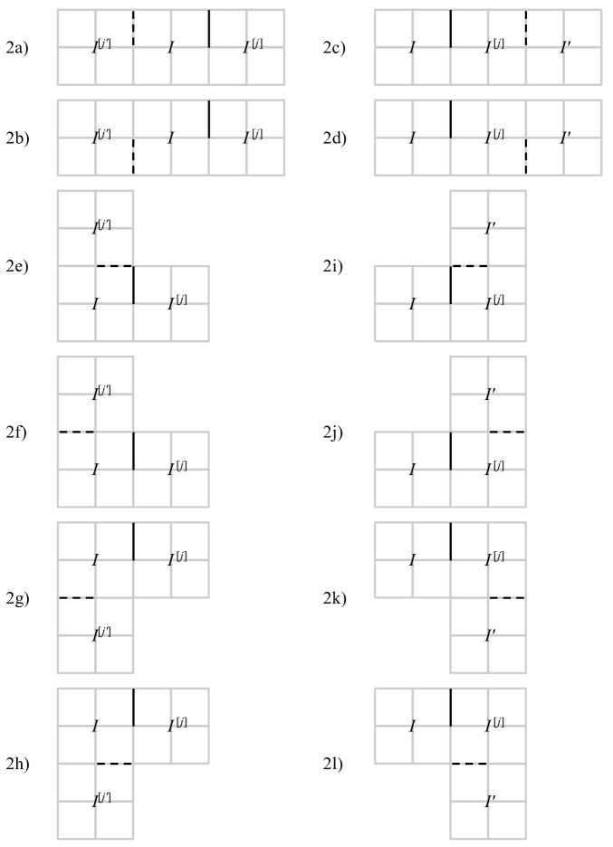
Figure 8: Subcases 2a through 2l. Links $(I,0,j)$ and $(I^{\prime},0,j^{\prime})$ are represented by the bold and dashed links, respectively.

Consider Subcases 2a, b, e, f, g, h. It is possible to regard the link $(I^{\prime},0,j^{\prime})$ as $(I,0,j^{\prime})$ if we identify cell $I^{\prime}$ with $I$. Define

$$E^{j,j^{\prime},i_{I}}(\Phi_{I},\Phi_{I^{[j]}},\Phi_{{I}^{[j^{\prime}]}})$$ (89)

$$= \zeta^{j}_{i_{I}}(\Phi_{I})\zeta^{[j]}_{0}(\Phi_{I^{[j]}})\zeta^{j^{\prime}}_{i_{I}}(\Phi_{I})\zeta^{[j^{\prime}]}_{0}(\Phi_{{I}^{[j^{\prime}]}})$$

$$\times\Bigl{[}R_{i_{I},0}(\Phi_{I},\Phi_{I^{[j]}})+R_{i_{I},0}(\Phi_{I},\Phi_{{I}^{[j^{\prime}]}})\Bigr{]}.\quad$$

Summing over the twenty external links gives

Subcase 2a, b, e, f, g, h (90)

$$= \sum_{i_{I}=1}^{7}\mu_{I,j}^{z}\mu_{I,j^{\prime}}^{z}\Biggl{[}U^{j,j^{\prime},i_{I}}_{++++|++++}\prod_{b\in{{I}^{[j^{\prime}]}}}\mathrm{1\!\!1}_{b}\cdot\prod_{b\in I}\mathrm{1\!\!1}_{b}\cdot\prod_{b\in{I^{[j]}}}\mathrm{1\!\!1}_{b}+U^{j,j^{\prime},i_{I}}_{+-+-|+-+-}\prod_{b\in{{I}^{[j^{\prime}]}}}\mu_{b}^{x}\cdot\prod_{b\in I}\mathrm{1\!\!1}_{b}\cdot\prod_{b\in{I^{[j]}}}\mathrm{1\!\!1}_{b}$$

$$-U^{j,j^{\prime},i_{I}}_{++++|----}\prod_{b\in{{I}^{[j^{\prime}]}}}\mathrm{1\!\!1}_{b}\cdot\prod_{b\in I}\mu^{x}_{b}\cdot\prod_{b\in{I^{[j]}}}\mathrm{1\!\!1}_{b}-U^{j,j^{\prime},i_{I}}_{+-+-|-+-+}\prod_{b\in{{I}^{[j^{\prime}]}}}\mu^{x}_{b}\cdot\prod_{b\in I}\mu^{x}_{b}\cdot\prod_{b\in{I^{[j]}}}\mathrm{1\!\!1}_{b}$$

$$-U^{j,j^{\prime},i_{I}}_{++--|++--}\prod_{b\in{{I}^{[j^{\prime}]}}}\mathrm{1\!\!1}_{b}\cdot\prod_{b\in I}\mathrm{1\!\!1}_{b}\cdot\prod_{b\in{I^{[j]}}}\mu^{x}_{b}-U^{j,j^{\prime},i_{I}}_{+--+|+--+}\prod_{b\in{{I}^{[j^{\prime}]}}}\mu^{x}_{b}\cdot\prod_{b\in I}\mathrm{1\!\!1}_{b}\cdot\prod_{b\in{I^{[j]}}}\mu^{x}_{b}$$

$$+U^{j,j^{\prime},i_{I}}_{++--|--++}\prod_{b\in{{I}^{[j^{\prime}]}}}\mathrm{1\!\!1}_{b}\cdot\prod_{b\in I}\mu^{x}_{b}\cdot\prod_{b\in{I^{[j]}}}\mu^{x}_{b}+U^{j,j^{\prime},i_{I}}_{+--+|-++-}\prod_{b\in{{I}^{[j^{\prime}]}}}\mu^{x}_{b}\cdot\prod_{b\in I}\mu^{x}_{b}\cdot\prod_{b\in{I^{[j]}}}\mu^{x}_{b}\Biggr{]},$$

where

$$U^{j,j^{\prime},i_{I}}_{\sigma_{1}\sigma_{2}\sigma_{3}\sigma_{4}|\sigma_{5}\sigma_{6}\sigma_{7}\sigma_{8}} = \frac{1}{8}\Bigl{[}\sigma_{1}E^{j,j^{\prime},i_{I}}(+,+,+)$$ (91)

$$+\sigma_{2}E^{j,j^{\prime},i_{I}}(+,+,-)$$

$$+\sigma_{3}E^{j,j^{\prime},i_{I}}(+,-,+)$$

$$+\sigma_{4}E^{j,j^{\prime},i_{I}}(+,-,-)$$

$$+\sigma_{5}E^{j,j^{\prime},i_{I}}(-,+,+)$$

$$+\sigma_{6}E^{j,j^{\prime},i_{I}}(-,+,-)$$

$$+\sigma_{7}E^{j,j^{\prime},i_{I}}(-,-,+)$$

$$+\sigma_{8}E^{j,j^{\prime},i_{I}}(-,-,-)\Bigr{]}.\quad$$

Define

$$U_{1}^{j,j^{\prime}} = \sum_{i_{I}=1}^{7}U^{j,j^{\prime},i_{I}}_{++++|++++}$$ (92a)

$$U_{2}^{j,j^{\prime}} = \sum_{i_{I}=1}^{7}U^{j,j^{\prime},i_{I}}_{+-+-|+-+-}$$ (92b)

$$= \sum_{i_{I}=1}^{7}U^{j,j^{\prime},i_{I}}_{++--|++--}$$ (92c)

$$U_{3}^{j,j^{\prime}} = \sum_{i_{I}=1}^{7}U^{j,j^{\prime},i_{I}}_{++++|----}$$ (92d)

$$U_{4}^{j,j^{\prime}} = \sum_{i_{I}=1}^{7}U^{j,j^{\prime},i_{I}}_{+-+-|-+-+}$$ (92e)

$$= \sum_{i_{I}=1}^{7}U^{j,j^{\prime},i_{I}}_{++--|--++}.$$ (92f)

We have checked that expressions (92b) and (92c), and expressions (92e) and (92f) are equivalent. Also,

$$\sum_{i_{I}=1}^{7}U^{j,j^{\prime},i_{I}}_{+--+|+--+} = 0$$ (93a)

$$\sum_{i_{I}=1}^{7}U^{j,j^{\prime},i_{I}}_{+--+|-++-} = 0.$$ (93b)

Thus,

Subcase 2a, b, e, f, g, h (94)

$$= \mu^{z}_{I,j}\mu^{z}_{I,j^{\prime}}[U_{1}^{j,j^{\prime}}$$

$$+U_{2}^{j,j^{\prime}}\Phi_{{I}^{[j^{\prime}]}}-U_{2}^{j,j^{\prime}}\Phi_{I^{[j]}}-U_{3}^{j,j^{\prime}}\Phi_{I}$$

$$-U_{4}^{j,j^{\prime}}\Phi_{{I}^{[j^{\prime}]}}\Phi_{I}+U_{4}^{j,j^{\prime}}\Phi_{I}\Phi_{I^{[j]}}].$$

Notice that the mapping

$$j \to [j]$$

$$j^{\prime} \to [j^{\prime}]$$

$$I \to {I^{[j]}}$$

$${I^{[j]}} \to I$$

$${{I}^{[j^{\prime}]}} \to I^{\prime}$$ (95)

converts the diagrams for Subcases 2a, b, e, f, g, and h into the diagrams for Subcases 2c, d, i, j, k, and l, respectively, up to a reflection in the plane. However, this reflection does not affect the mathematical expression since it does not alter the relative locations of links. Applying rules (95) to Eq. (94) and remembering that now we cannot identify cells $I^{\prime}$ and $I$, yields

Subcase 2c, d, i, j, k, l (96)

$$= \mu^{z}_{I,j}\mu^{z}_{I^{\prime},j^{\prime}}[U_{1}^{[j],[j^{\prime}]}$$

$$+U_{2}^{[j],[j^{\prime}]}\Phi_{I^{\prime}}-U_{2}^{[j],[j^{\prime}]}\Phi_{I}-U_{3}^{[j],[j^{\prime}]}\Phi_{I^{[j]}}$$

$$-U_{4}^{[j],[j^{\prime}]}\Phi_{I^{\prime}}\Phi_{I^{[j]}}+U_{4}^{[j],[j^{\prime}]}\Phi_{I^{[j]}}\Phi_{I}].$$

A.5 Renormalized spin-$\tfrac{1}{2}$ operators

Since each link $B$ of the new lattice corresponds to two links of a cell, say $b$ and $b^{\prime}$, a prescription is needed to define new link operators $\{X_{B},\,Z_{B}\}$ from the old ones $\{\mu^{x}_{b},\,\mu^{z}_{b}\}$ and $\{\mu^{x}_{b^{\prime}},\,\mu^{z}_{b^{\prime}}\}$. Although it appears that external links $b$ and $b^{\prime}$ have two qubits worth of freedom, Fradkin and Raby showed that gauge invariance restricts this freedom to just one. Here we translate their argument into a format that comports with the perturbative framework of Hirsch and Mazenko.

Consider the site at the midpoint of the boundary between cells $I$ and $I+\hat{x}$ in Fig. 6. The generator of gauge transformations at this site is $G_{\sigma}=\sigma^{z}_{I,0,1}\sigma^{z}_{I,0,8}\sigma^{z}_{I,1,0}\sigma^{z}_{I+\hat{x},3,0}$. Physical states in Hilbert space must satisfy $G_{\sigma}=+1$. Since $[G_{\sigma},H_{\sigma}^{0}]=0$, the bi-vector-valued quantity $T_{0}=\sum_{i}|i\rangle\otimes|\mu_{i}\rangle$ must satisfy

$$T_{0}=G_{\sigma}T_{0}.$$ (97)

Whence does $T_{0}$ come? Briefly, according to Ref. Hirsch and Mazenko, 1979, $T_{0}$ is the lowest-order-in-$g$ approximation to $T[\mu|\sigma]$, which is a vector-to-vector projection operator that allows the renormalized Hamiltonian to be computed by a trace. In Eq. (2.5) $T_{0}$ is seen to satisfy a normalization constraint, $\mathrm{Tr}\,_{\sigma}(T_{0}T_{0}^{\dagger})=\mathrm{1\!\!1}_{\mu}$. This is equivalent to

$$\mathrm{1\!\!1}_{\mu}=\mathrm{Tr}\,_{\sigma}(G_{\sigma}T_{0}T_{0}^{\dagger})=\sum_{i,i^{\prime}}\langle i^{\prime}|G_{\sigma}|i\rangle|\mu_{i}\rangle\langle\mu_{i}|,$$ (98)

with the second equality following from $\langle i|\alpha\rangle=0$. Simply put, the identity operator in the reduced Hilbert space can be computed by restricting $G_{\sigma}$ to the subspace $\{|i\rangle\}$ of lattice eigenstates formed by cell ground states; the orthogonal subspace $\{|\alpha\rangle\}$ is completely overlooked by the projector $T_{0}$. Using Eq. (52),

$$G_{\sigma}|i\rangle = |0(-x_{I,1},-x_{I,8})\rangle_{I}|0(-x_{I+\hat{x},4},-x_{I+\hat{x},5})\rangle_{I+\hat{x}}$$ (99)

$$|-x_{I,1}\rangle_{I,0,1}|-x_{I,8}\rangle_{I,0,8}\dotsb,$$

where ellipses represent cell and external link states that are not acted upon by $G_{\sigma}$. Note that $x_{I+\hat{x},4}=x_{I,1}$ and $x_{I+\hat{x},5}=x_{I,8}$. When $\langle i^{\prime}|$ is applied to Eq. (99), the resulting matrix element is nonzero only if $x^{\prime}_{I,0,1}=-x_{I,0,1}$ and $x^{\prime}_{I,0,8}=-x_{I,0,8}$, with all other $x^{\prime}_{b}=x_{b}$. If this holds, then the matrix element is unity. This constraint collapses the sum over $i^{\prime}$. Performing the remaining sum over $i$ then leads to

$$\sum_{x_{I,1}=\pm}|x_{I,1}\rangle\langle-x_{I,1}|\sum_{x_{I,8}=\pm}|x_{I,8}\rangle\langle-x_{I,8}|=\mu^{z}_{I,1}\mu^{z}_{I,8},$$ (100)

with implicit identities on all other external links. Thus, we have proven that

$$\mu^{z}_{I,1}\mu^{z}_{I,8}=\mathrm{1\!\!1}_{\mu}.$$ (101)

Therefore, $\mu^{z}_{I,1}=\mu^{z}_{I,8}$ on the reduced Hilbert space of the thinned lattice.

Define renormalized link operators

$$X_{B}=\mu^{x}_{b}\mu^{x}_{b^{\prime}},\qquad Z_{B}=(\mu^{z}_{b}+\mu^{z}_{b^{\prime}})/2,$$ (102)

where $b$ and $b^{\prime}$ are the two contiguous links from the same edge $B$ of a cell. See Fig. 9. It is easily checked that they reproduce the Pauli algebra $X_{B}Z_{B}=-Z_{B}X_{B}$, $X_{B}^{2}=\mathrm{1\!\!1}_{B}$, and $Z_{B}^{2}=\mathrm{1\!\!1}_{B}$. Note that the identity $\mu^{z}_{b}\mu^{z}_{b^{\prime}}=\mathrm{1\!\!1}_{B}$ implies that $Z_{B}=\mu_{b}^{z}=\mu_{b^{\prime}}^{z}$.

Cells become plaquettes in the thinned lattice. For these we define the magnetic flux in the obvious way,

$$\Phi_{I}=\prod_{B\in\partial I}X_{B}.$$ (103)

A.6 Renormalized Hamiltonian

In terms of the renormalized spin-$\tfrac{1}{2}$ operators, Eq. (67c) reads

$$H^{(0)}_{\mu}=\frac{\epsilon_{0}^{\text{c}}(+)+\epsilon_{0}^{\text{c}}(-)}{2}\frac{N_{\text{plaq}}}{4}-\frac{\epsilon_{0}^{\text{c}}(-)-\epsilon_{0}^{\text{c}}(+)}{2}\sum_{I}\Phi_{I},$$ (104)

where $N_{\text{plaq}}$ is the number of plaquettes in the original lattice. And for Eq. (68e) we make a minor notational change: instead of referring to links as “$I,j$” we use “$B$,”

$$H^{(1)}_{\mu}=-2h|\langle 0_{-}|0_{+}\rangle_{I}|^{2}\sum_{B}Z_{B}.$$ (105)

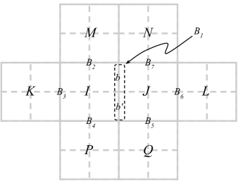
Figure 9: Cells involved in effective operators generated at second order in the intercell coupling. Cells $I,\,J,\,K,\,L,\,M,\,N,\,P,\,Q$ become the plaquettes of the thinned lattice once internal links (dashed) are decimated. External links (solid) $b$ and $b^{\prime}$ comprise the link $B_{1}$ in the thinned lattice.

We are not quite ready to write a gauge-invariant expression for $H^{(2)}_{\mu}$. First, Eq. (75) needs to be assembled by combining all subcases from Cases 1 and 2. Since pairs of contiguous links that form the edge of a cell will eventually become a single link $B$ in the thinned lattice, it is convenient to reduce the scope of the sum as

$$H^{(2)}_{\mu}=\frac{h^{2}}{2}\sum_{B}(\text{Case 1}+\text{Case 2})_{j=1}+(\text{Case 1}+\text{Case 2})_{j=8}.$$ (106)

Note that we could have also picked the pair $j=2,3$, or $4,5$, or $6,7$. However, this choice is immaterial due to the $90^{\circ}$ rotation symmetry of the lattice. Also, the choice $j=1,8$ matches the links labeled $b,b^{\prime}$ in Fig. 9 whose simplified notation we henceforth employ. Accordingly, for Case 1 we have $\text{Subcase 1a}=S_{1}+S_{2}\Phi_{I}\Phi_{J}-S_{3}(\Phi_{I}+\Phi_{J})$ and $\text{Subcase 1b}=T_{1}+T_{2}\Phi_{I}\Phi_{J}-T_{2}(\Phi_{I}+\Phi_{J})$ because $\mu^{z}_{b}\mu^{z}_{b^{\prime}}=\mathrm{1\!\!1}_{B}$. For Case 2, we must be careful to properly overlay Fig. 9 onto each diagram shown in Fig. 8 so that the cells labeled “$I$” coincide. For instance, consider Subcase 2c with $j=1$. Then ${I^{[j]}}=J$, $I^{\prime}=L$, and $j^{\prime}=4$. Therefore,

$$(\text{Subcase 2c})_{j=1} = Z_{B_{1}}Z_{B_{6}}[U_{1}^{[1],[4]}$$ (107)

$$+U_{2}^{[1],[4]}\Phi_{L}-U_{2}^{[1],[4]}\Phi_{I}-U_{3}^{[1],[4]}\Phi_{J}$$

$$-U_{4}^{[1],[4]}\Phi_{L}\Phi_{J}+U_{4}^{[1],[4]}\Phi_{J}\Phi_{I}].\quad\qquad$$

By using relations (39) we can set $[1]=4$ and $[4]=1$. For another example, consider Subcase 2f with $j=8$. The diagram for this may be obtained by reflecting diagram 2f in Fig. 8 about a horizontal line. Overlaying Fig. 9 then gives ${I^{[j]}}=J$, ${{I}^{[j^{\prime}]}}=P$, and $j^{\prime}=6$. Therefore,

$$(\text{Subcase 2f})_{j=8} = Z_{B_{1}}Z_{B_{4}}[U_{1}^{8,6}$$ (108)

$$+U_{2}^{8,6}\Phi_{P}-U_{2}^{8,6}\Phi_{J}-U_{3}^{8,6}\Phi_{I}$$

$$-U_{4}^{8,6}\Phi_{P}\Phi_{I}+U_{4}^{8,6}\Phi_{I}\Phi_{J}].\qquad$$

In order to combine all subcases under Case 2 define

$$V_{k} = U_{k}^{1,2}+U_{k}^{1,3}+U_{k}^{8,3}+U_{k}^{8,2}$$

$$= U_{k}^{1,6}+U_{k}^{1,7}+U_{k}^{8,7}+U_{k}^{8,6}$$

$$= U_{k}^{4,3}+U_{k}^{4,2}+U_{k}^{5,2}+U_{k}^{5,3}$$

$$= U_{k}^{4,7}+U_{k}^{4,6}+U_{k}^{5,6}+U_{k}^{5,7},$$

$$W_{k} = U_{k}^{1,4}+U_{k}^{1,5}+U_{k}^{8,5}+U_{k}^{8,4}$$

$$= U_{k}^{4,1}+U_{k}^{4,8}+U_{k}^{5,8}+U_{k}^{5,1},$$

for $k=1,\dotsc,4$. Notice that $V_{k}$ are coefficients from terms in which $Z$’s reside on nearest-neighbor (i.e., diagonally adjacent) links, whereas $W_{k}$ are coefficients from terms in which $Z$’s reside on next-nearest-neighbor (i.e., directly opposite) links. The contribution from link $B_{1}$ is

$$(\text{Case 1}+\text{Case 2})_{B_{1}} = 2(S_{1}+T_{1})+2(S_{2}+T_{2})\Phi_{I}\Phi_{J}-2(S_{3}+T_{3})(\Phi_{I}+\Phi_{J})$$ (111)

$$+Z_{B_{1}}Z_{B_{2}}[V_{1}+V_{2}\Phi_{M}-V_{2}\Phi_{J}-V_{3}\Phi_{I}-V_{4}\Phi_{M}\Phi_{I}+V_{4}\Phi_{I}\Phi_{J}]$$

$$+Z_{B_{1}}Z_{B_{4}}[V_{1}+V_{2}\Phi_{P}-V_{2}\Phi_{J}-V_{3}\Phi_{I}-V_{4}\Phi_{P}\Phi_{I}+V_{4}\Phi_{I}\Phi_{J}]$$

$$+Z_{B_{1}}Z_{B_{5}}[V_{1}+V_{2}\Phi_{Q}-V_{2}\Phi_{I}-V_{3}\Phi_{J}-V_{4}\Phi_{Q}\Phi_{J}+V_{4}\Phi_{J}\Phi_{I}]$$

$$+Z_{B_{1}}Z_{B_{7}}[V_{1}+V_{2}\Phi_{N}-V_{2}\Phi_{I}-V_{3}\Phi_{J}-V_{4}\Phi_{N}\Phi_{J}+V_{4}\Phi_{J}\Phi_{I}]$$

$$+Z_{B_{1}}Z_{B_{3}}[W_{1}+W_{2}\Phi_{K}-W_{2}\Phi_{J}-W_{3}\Phi_{I}-W_{4}\Phi_{K}\Phi_{I}+W_{4}\Phi_{I}\Phi_{J}]$$

$$+Z_{B_{1}}Z_{B_{6}}[W_{1}+W_{2}\Phi_{L}-W_{2}\Phi_{I}-W_{3}\Phi_{J}-W_{4}\Phi_{L}\Phi_{J}+W_{4}\Phi_{J}\Phi_{I}].$$

Observe that not all of these terms are hermitian. For example, $(Z_{B_{1}}Z_{B_{3}}\Phi_{K})^{\dagger}=\Phi_{K}Z_{B_{3}}Z_{B_{1}}=-Z_{B_{1}}Z_{B_{3}}\Phi_{K}$ because $X_{B_{3}}$ anticommutes with $Z_{B_{3}}$. Such terms must disappear when we add similar contributions from the other links. For instance, if we look at $(\text{Case 1}+\text{Case 2})_{B_{3}}$ then we also get a term prefaced with $Z_{B_{3}}Z_{B_{1}}$. Combining like terms eliminates non-hermitian operators. In particular, operators with coefficients $V_{k}$ and $W_{k}$ for $k=2,4$ vanish.

For any pair of nearest-neighbor links $B$ and $B^{\prime}$ at right angles (denoted $B\perp B^{\prime}$), $H^{(2)}_{\mu}$ contains operators of the form

$$h^{2}Z_{B}Z_{B^{\prime}}(V_{1}-V_{3}\Phi_{I}),$$ (112)

where plaquette $I$ is bounded by links $B$ and $B^{\prime}$. We might say that $I$ sits in the “elbow” of the hook made by $B$ and $B^{\prime}$.

For any pair of next-nearest-neighbor links $B$ and $B^{\prime}$ directly opposite from each other (denoted $B\parallel B^{\prime}$), $H^{(2)}_{\mu}$ contains operators of the form

$$h^{2}Z_{B}Z_{B^{\prime}}(W_{1}-W_{3}\Phi_{I}),$$ (113)

where plaquette $I$ is bounded by links $B$ and $B^{\prime}$. We might say that $I$ is “sandwiched” in-between $B$ and $B^{\prime}$.

The full second-order correction is

$$H^{(2)}_{\mu} = 2h^{2}(S_{1}+T_{1})\frac{N_{\text{plaq}}}{4}+h^{2}(S_{2}+T_{2})\sum_{\langle I,J\rangle}\Phi_{I}\Phi_{J}-4h^{2}(S_{3}+T_{3})\sum_{I}\Phi_{I}$$ (114)

$$+h^{2}V_{1}\sum_{B\perp B^{\prime}}Z_{B}Z_{B^{\prime}}-h^{2}V_{3}\sum_{B\perp B^{\prime}}Z_{B}Z_{B^{\prime}}\Phi_{I_{\text{elbow}}}+h^{2}W_{1}\sum_{B\parallel B^{\prime}}Z_{B}Z_{B^{\prime}}-h^{2}W_{3}\sum_{B\parallel B^{\prime}}Z_{B}Z_{B^{\prime}}\Phi_{I_{\text{sandwiched}}},\qquad$$

where $\langle I,J\rangle$ denotes nearest-neighbor plaquettes $I$ and $J$. It is important to remark that all operators $Z_{B}Z_{B^{\prime}}$ associated to hooks $B\perp B^{\prime}$ are being summed over, even those that may be gauge-equivalent to others. The effective operators generated by renormalization are depicted in Fig. 3.

Inspection of Eq. (114) reveals five new gauge-invariant effective operators that have been generated by the renormalization transformation. The coefficients of these new operators will influence those obtained by successive iterations of the decimation procedure. Therefore, we must go back and include these operators in $H_{\sigma}$. We choose to append them to $V_{\sigma}$ in Eq. (40) so that the eigenvalue problem on each cell remains unchanged. Using the notation of Fig. 3,

$$\text{add to $V_{\sigma}$}=\sum_{\alpha=1}^{5}K_{\alpha}\mathcal{O}_{\alpha}+FN_{\text{plaq}}.$$ (115)

As in Refs. Hirsch and Mazenko, 1979 and Hirsch, 1979 we treat the coefficients $K_{\alpha}$ as being $O(h^{2})$ since they are generated at second order in Hirsch–Mazenko perturbation theory. This means that we need only compute the analogue of Eq. (66c),

$$\text{add to $H_{\mu}^{\text{ren}}$}=\sum_{i,i^{\prime}}\langle i^{\prime}|(\text{add to $V_{\sigma}$})|i\rangle|\mu_{i}\rangle\langle\mu_{i^{\prime}}|.$$ (116)

For the identity operator, a single renormalization step reduces the number of plaquettes by a factor of 4. Therefore, $F^{\prime}=4F$.

Consider $\sum_{i,i^{\prime}}\langle i^{\prime}|\mathcal{O}_{\alpha}|i\rangle|\mu_{i}\rangle\langle\mu_{i^{\prime}}|$. Generically, $\mathcal{O}_{\alpha}$ consists of a product of $Z$’s and $X$’s (or $\sigma^{z}$’s and $\sigma^{x}$’s in the original Hilbert space). Depending on how this operator is situated on the lattice some of the spin operators will act on internal links of a cell and some will act on external links. Since operators on different links commute, we can always write $\mathcal{O}_{\alpha}$ as a product of operators—one referring to internal links only and the other referring to external links only. Let $\mathcal{O}_{\alpha}=\mathcal{O}^{\text{int}}_{\alpha}\mathcal{O}^{\text{ext}}_{\alpha}$. Since internal links always belong to a specific cell, we may further decompose $\mathcal{O}^{\text{int}}_{\alpha}=\prod_{I}\mathcal{O}_{\alpha}^{\text{int $I$}}$, where $I$ is the cell index. Then

$$\langle i^{\prime}|\mathcal{O}_{\alpha}|i\rangle = \prod_{I}\langle 0(\{x^{\prime}\})|\mathcal{O}_{\alpha}^{\text{int $I$}}|0(\{x\})\rangle_{I}$$ (117)

$$\times\langle x^{\prime}|\dotsb\langle x^{\prime}|\mathcal{O}^{\text{ext}}_{\alpha}|x\rangle\dotsb|x\rangle,$$

where all external links $x$ and $x^{\prime}$ are involved in the matrix element. If we now perform $\sum_{i^{\prime}}$, which amounts to summing over all possible configurations of the external links $x^{\prime}$, then any external link not directly touched by $\mathcal{O}_{\alpha}^{\text{ext}}$ will receive a Kronecker delta setting $x^{\prime}=x$. Since $|\mu_{i}\rangle\langle\mu_{i^{\prime}}|=\prod|x\rangle\langle x^{\prime}|$, $|x\rangle\langle x^{\prime}|$ corresponding to untouched links become $|x\rangle\langle x|$. Next, when $\sum_{i}$ is performed we might expect to get $\sum_{x=\pm}|x\rangle\langle x|=\mathrm{1\!\!1}$ for those untouched external links. However, this is only true if another condition is met: those untouched external links must not lie on a cell that contains a touched link somewhere else on its border or has $\mathcal{O}^{\text{int}}_{\alpha}$ acting on it. We shall refer to such cells as “touched” cells. Otherwise, there will be a non-unit matrix element factor sitting inside the sum $\sum_{x=\pm}$. Our calculational algorithm can be stated as

$$\sum_{i,i^{\prime}}\langle i^{\prime}|\mathcal{O}_{\alpha}|i\rangle|\mu_{i}\rangle\langle\mu_{i^{\prime}}|$$ (118)

$$= \underbrace{\sum_{x}\dotsc\sum_{x}}_{\begin{subarray}{c}\text{directly touched}\\ \text{external links}\end{subarray}}\underbrace{\sum_{x}\dotsc\sum_{x}}_{\begin{subarray}{c}\text{untouched}\\ \text{external links}\\ \text{on a touched cell}\end{subarray}}\underbrace{\sum_{x^{\prime}}\dotsc\sum_{x^{\prime}}}_{\begin{subarray}{c}\text{directly touched}\\ \text{external links}\end{subarray}}\prod_{\text{touched cells $I$}}$$

$$\langle 0(\{x^{\prime}\})|\mathcal{O}_{\alpha}^{\text{int $I$}}|0(\{x\})\rangle_{I}\Bigr{|}_{\text{$x^{\prime}=x$ for untouched links}}$$

$$\times\underbrace{\langle x^{\prime}|\dotsb\langle x^{\prime}|}_{\begin{subarray}{c}\text{directly touched}\\ \text{external links}\end{subarray}}\mathcal{O}^{\text{ext}}_{\alpha}\underbrace{|x\rangle\dotsb|x\rangle}_{\begin{subarray}{c}\text{directly touched}\\ \text{external links}\end{subarray}}$$

$$\times\underbrace{|x\rangle\langle x^{\prime}|\dotsb|x\rangle\langle x^{\prime}|}_{\begin{subarray}{c}\text{directly touched}\\ \text{external links}\end{subarray}}\cdot\underbrace{|x\rangle\langle x|\dotsb|x\rangle\langle x|}_{\begin{subarray}{c}\text{untouched}\\ \text{external links}\\ \text{on a touched cell}\end{subarray}}.$$

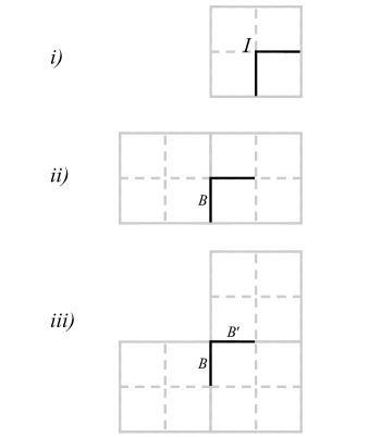
Figure 10: How $\mathcal{O}_{1}$ generates effective operators.

Direct computation of expression (116) is straightforward using Eq. (118) but tedious. As an example, consider $\mathcal{O}_{1}$. There are three qualitatively distinct ways it can cover the original lattice. See Fig. 10. In Case (i) the hook lies entirely on internal links. Define

$$\chi=\langle 0(\{A\})|\sigma^{z}_{I,1,0}\sigma^{z}_{I,4,0}|0(\{A\}\rangle_{I}.$$ (119)

It turns out that $\chi$ is a function of the flux $\Phi_{I}=\prod_{k=1}^{4}A_{k}$ only. Therefore,

$$\chi(+) = \langle 0_{+}|\sigma^{z}_{I,1,0}\sigma^{z}_{I,4,0}|0_{+}\rangle_{I},$$ (120a)

$$\chi(-) = \langle 0_{-}|\sigma^{z}_{I,1,0}\sigma^{z}_{I,4,0}|0_{-}\rangle_{I}.$$ (120b)

Thus,

Case (i) $$= 4K_{1}\frac{\chi(+)+\chi(-)}{2}\frac{N_{\text{plaq}}}{4}$$ (121)

$$+4K_{1}\frac{\chi(+)-\chi(-)}{2}\sum_{I}\Phi_{I}.$$

There is a factor of 4 because there are four different orientations in which the hook can lie entirely inside the plaquette. In Case (ii) the hook can lie in one of four ways on the shared boundary between two plaquettes. So

$$\text{Case ({ii})}=4K_{1}|\langle 0_{-}|0_{+}\rangle_{I}|^{2}\sum_{B}Z_{B}.$$ (122)

In Case (iii) there is only a single orientation of the hook that straddles all three plaquettes. So

$$\text{Case ({iii})}=K_{1}|\langle 0_{-}|0_{+}\rangle_{I}|^{2}\sum_{B\perp B^{\prime}}Z_{B}Z_{B^{\prime}}.$$ (123)

The contributions from $\mathcal{O}_{\alpha}$ for $\alpha=2,\dotsc,5$ may be worked out in a similar fashion.

Before writing the full expression for (116) it will be convenient to adopt some shorthand notation. Internal-link spin operators, which are normally denoted $\vec{\sigma}_{I,i,0}$, will be shortened to $\vec{\sigma}_{i}$. External-link spin operators will not appear explicitly in the matrix elements so there is no chance of confusion. And we shall suppress the subscript $I$ on matrix elements. We find

add to $$H_{\mu}^{\text{ren}} = \frac{N_{\text{plaq}}}{4}\Bigl{[}4F+2K_{1}(\langle 0_{+}|\sigma^{z}_{1}\sigma^{z}_{4}|0_{+}\rangle+\langle 0_{-}|\sigma^{z}_{1}\sigma^{z}_{4}|0_{-}\rangle)+2K_{2}(\langle 0_{+}|\sigma^{z}_{1}\sigma^{z}_{2}\sigma^{x}_{1}\sigma^{x}_{2}|0_{+}\rangle+\langle 0_{-}|\sigma^{z}_{1}\sigma^{z}_{2}\sigma^{x}_{1}\sigma^{x}_{2}|0_{-}\rangle)$$ (124)

$$\qquad\qquad+2K_{5}\bigl{(}\langle 0_{+}|\sigma^{x}_{1}\sigma^{x}_{3}|0_{+}\rangle+\tfrac{1}{4}(\langle 0_{+}|\sigma^{x}_{1}\sigma^{x}_{2}|0_{+}\rangle^{2}+2\langle 0_{+}|\sigma^{x}_{1}\sigma^{x}_{2}|0_{+}\rangle\langle 0_{-}|\sigma^{x}_{1}\sigma^{x}_{2}|0_{-}\rangle+\langle 0_{-}|\sigma^{x}_{1}\sigma^{x}_{2}|0_{-}\rangle^{2})\bigr{)}\Bigr{]}$$

$$+\sum_{B}Z_{B}\Bigl{[}4K_{1}|\langle 0_{-}|0_{+}\rangle|^{2}+4K_{2}\langle 0_{-}|0_{+}\rangle\langle 0_{-}|\sigma^{x}_{1}\sigma^{x}_{2}|0_{+}\rangle+4K_{3}|\langle 0_{-}|0_{+}\rangle|^{2}+4K_{4}\langle 0_{-}|0_{+}\rangle\langle 0_{-}|\sigma^{x}_{1}\sigma^{x}_{2}|0_{+}\rangle\Bigr{]}$$

$$+\sum_{I}\Phi_{I}\Bigl{[}2K_{1}(\langle 0_{+}|\sigma^{z}_{1}\sigma^{z}_{4}|0_{+}\rangle-\langle 0_{-}|\sigma^{z}_{1}\sigma^{z}_{4}|0_{-}\rangle)+2K_{2}(\langle 0_{+}|\sigma^{z}_{1}\sigma^{z}_{2}\sigma^{x}_{1}\sigma^{x}_{2}|0_{+}\rangle-\langle 0_{-}|\sigma^{z}_{1}\sigma^{z}_{2}\sigma^{x}_{1}\sigma^{x}_{2}|0_{-}\rangle)$$

$$\qquad\qquad+2K_{5}(\langle 0_{+}|\sigma^{x}_{1}\sigma^{x}_{3}|0_{+}\rangle+\langle 0_{+}|\sigma^{x}_{1}\sigma^{x}_{2}|0_{+}\rangle^{2}-\langle 0_{-}|\sigma^{x}_{1}\sigma^{x}_{2}|0_{-}\rangle^{2})\Bigr{]}$$

$$+\sum_{B\perp B^{\prime}}Z_{B}Z_{B^{\prime}}\Bigl{[}K_{1}|\langle 0_{-}|0_{+}\rangle|^{2}+\tfrac{1}{2}K_{2}|\langle 0_{-}|0_{+}\rangle|^{2}(\langle 0_{+}|\sigma^{x}_{1}\sigma^{x}_{2}|0_{+}\rangle+\langle 0_{-}|\sigma^{x}_{1}\sigma^{x}_{2}|0_{-}\rangle)\Bigr{]}$$

$$+\sum_{B\perp B^{\prime}}Z_{B}Z_{B^{\prime}}\Phi_{I_{\text{elbow}}}\Bigl{[}\tfrac{1}{2}K_{2}|\langle 0_{-}|0_{+}\rangle|^{2}(\langle 0_{+}|\sigma^{x}_{1}\sigma^{x}_{2}|0_{+}\rangle-\langle 0_{-}|\sigma^{x}_{1}\sigma^{x}_{2}|0_{-}\rangle)\Bigr{]}$$

$$+\sum_{\langle I,J\rangle}\Phi_{I}\Phi_{J}\Bigl{[}\tfrac{1}{2}K_{5}(\langle 0_{+}|\sigma^{x}_{1}\sigma^{x}_{2}|0_{+}\rangle^{2}-2\langle 0_{+}|\sigma^{x}_{1}\sigma^{x}_{2}|0_{+}\rangle\langle 0_{-}|\sigma^{x}_{1}\sigma^{x}_{2}|0_{-}\rangle+\langle 0_{-}|\sigma^{x}_{1}\sigma^{x}_{2}|0_{-}\rangle^{2})\Bigr{]}$$

All matrix elements appearing above have been written in terms of $|0_{\pm}\rangle$ as given by Eqs. (68c) and (68d). It is worth noting that expression (124) with the alternative definition $|0_{-}\rangle_{I}=|0(A_{1}=-,A_{2}=+,A_{3}=+,A_{4}=+)\rangle_{I}$ would not be correct.

The renormalized Hamiltonian to second order in the coupling $h$ is given by adding expressions (104), (105), (114), and (124). This yields

$$H^{\text{ren}}_{\mu} = -h^{\prime}\sum_{B}Z_{B}-J^{\prime}\sum_{I}\Phi_{I}$$ (125a)

$$+K_{1}^{\prime}\sum_{B\perp B^{\prime}}Z_{B}Z_{B^{\prime}}+K_{2}^{\prime}\sum_{B\perp B^{\prime}}Z_{B}Z_{B^{\prime}}\Phi_{I_{\text{elbow}}}+K_{3}^{\prime}\sum_{B\parallel B^{\prime}}Z_{B}Z_{B^{\prime}}+K_{4}^{\prime}\sum_{B\parallel B^{\prime}}Z_{B}Z_{B^{\prime}}\Phi_{I_{\text{sandwiched}}}+K_{5}^{\prime}\sum_{\langle I,J\rangle}\Phi_{I}\Phi_{J}$$

$$+F^{\prime}\frac{N_{\text{plaq}}}{4},$$

where

$$h^{\prime} = 2|\langle 0_{-}|0_{+}\rangle|^{2}(h-2K_{1}-2K_{3})-4\langle 0_{-}|0_{+}\rangle\langle 0_{-}|\sigma^{x}_{1}\sigma^{x}_{2}|0_{+}\rangle(K_{2}+K_{4})$$ (125b)

$$J^{\prime} = \frac{\epsilon^{\text{c}}_{0}(-)-\epsilon^{\text{c}}_{0}(+)}{2}+4h^{2}(S_{3}+T_{3})+2K_{1}(\langle 0_{-}|\sigma^{z}_{1}\sigma^{z}_{4}|0_{-}\rangle-\langle 0_{+}|\sigma^{z}_{1}\sigma^{z}_{4}|0_{+}\rangle)$$ (125c)

$$+2K_{2}(\langle 0_{-}|\sigma^{z}_{1}\sigma^{z}_{2}\sigma^{x}_{1}\sigma^{x}_{2}|0_{-}\rangle-\langle 0_{+}|\sigma^{z}_{1}\sigma^{z}_{2}\sigma^{x}_{1}\sigma^{x}_{2}|0_{+}\rangle)$$

$$+2K_{5}(\langle 0_{-}|\sigma^{x}_{1}\sigma^{x}_{2}|0_{-}\rangle^{2}-\langle 0_{+}|\sigma^{x}_{1}\sigma^{x}_{3}|0_{+}\rangle-\langle 0_{+}|\sigma^{x}_{1}\sigma^{x}_{2}|0_{+}\rangle^{2})$$

$$K_{1}^{\prime} = h^{2}V_{1}+|\langle 0_{-}|0_{+}\rangle|^{2}\bigl{(}K_{1}+\tfrac{1}{2}K_{2}(\langle 0_{+}|\sigma^{x}_{1}\sigma^{x}_{2}|0_{+}\rangle+\langle 0_{-}|\sigma^{x}_{1}\sigma^{x}_{2}|0_{-}\rangle)\bigr{)}$$ (125d)

$$K_{2}^{\prime} = -h^{2}V_{3}+\tfrac{1}{2}K_{2}|\langle 0_{-}|0_{+}\rangle|^{2}(\langle 0_{+}|\sigma^{x}_{1}\sigma^{x}_{2}|0_{+}\rangle-\langle 0_{-}|\sigma^{x}_{1}\sigma^{x}_{2}|0_{-}\rangle)$$ (125e)

$$K_{3}^{\prime} = h^{2}W_{1}$$ (125f)

$$K_{4}^{\prime} = -h^{2}W_{3}$$ (125g)

$$K_{5}^{\prime} = h^{2}(S_{2}+T_{2})+\tfrac{1}{2}K_{5}(\langle 0_{+}|\sigma^{x}_{1}\sigma^{x}_{2}|0_{+}\rangle-\langle 0_{-}|\sigma^{x}_{1}\sigma^{x}_{2}|0_{-}\rangle)^{2}$$ (125h)

$$F^{\prime} = \frac{\epsilon_{0}^{\text{c}}(+)+\epsilon_{0}^{\text{c}}(-)}{2}+2h^{2}(S_{1}+T_{1})+4F+2K_{1}(\langle 0_{+}|\sigma^{z}_{1}\sigma^{z}_{4}|0_{+}\rangle+\langle 0_{-}|\sigma^{z}_{1}\sigma^{z}_{4}|0_{-}\rangle)$$ (125i)

$$+2K_{2}(\langle 0_{+}|\sigma^{z}_{1}\sigma^{z}_{2}\sigma^{x}_{1}\sigma^{x}_{2}|0_{+}\rangle+\langle 0_{-}|\sigma^{z}_{1}\sigma^{z}_{2}\sigma^{x}_{1}\sigma^{x}_{2}|0_{-}\rangle)$$

$$+2K_{5}\bigl{(}\langle 0_{+}|\sigma^{x}_{1}\sigma^{x}_{3}|0_{+}\rangle+\tfrac{1}{4}(\langle 0_{+}|\sigma^{x}_{1}\sigma^{x}_{2}|0_{+}\rangle+\langle 0_{-}|\sigma^{x}_{1}\sigma^{x}_{2}|0_{-}\rangle)^{2}\bigr{)}.$$

The matrix elements appearing above may be calculated using the cell-basis representations for internal $\sigma^{z}$ matrices given in Eqs. (53), and

$$\sigma^{x}_{1}\sigma^{x}_{2} = \begin{pmatrix}&&&&0&1&0&0\\ &&&&0&0&0&1\\ &&&&0&0&1&0\\ &&&&1&0&0&0\\ 0&0&0&1&&&&\\ 1&0&0&0&&&&\\ 0&0&1&0&&&&\\ 0&1&0&0&&&&\end{pmatrix},$$ (126a)

$$\sigma^{x}_{1}\sigma^{x}_{3} = \begin{pmatrix}0&0&1&0&&&&\\ 0&0&0&1&&&&\\ 1&0&0&0&&&&\\ 0&1&0&0&&&&\\ &&&&0&0&0&1\\ &&&&0&0&1&0\\ &&&&0&1&0&0\\ &&&&1&0&0&0\end{pmatrix}.$$ (126b)

Eqs. (125) are recursion relations for the operator coefficients in the Hamiltonian. We have checked that they are equivalent to the recursion relations derived by Hirsch in Ref. Hirsch, 1979 for the quantum Hamiltonian of the square-lattice Ising model in a transverse magnetic field. This check is accomplished using a duality transformation. Kogut (1979) The ’t Hooft disorder operator, given by a string of $\sigma^{z}$’s in the lattice gauge theory, corresponds to the order parameter, $\sigma^{x}$, in the Ising model. And the magnetic flux operator, given by a product of $\sigma^{x}$’s around a plaquette, maps to the transverse field operator, $\sigma^{z}$, living at the site dual to the plaquette.

It is certainly more challenging to obtain the recursion relations in the lattice gauge theory than in the Ising model—gauge invariance enlarges the number of possible states, and additional formalism is necessary to restrict to the gauge-invariant sector. For instance, in the former one is forced to consider the cellular magnetic flux $\Phi_{I}$ as potentially dependent on eight boundary conditions, whereas in the Ising model no such boundary conditions are required. The fact that our results agree with those obtained from the simpler (non-gauged) formulation of the theory is a reassuring check that we correctly implemented the Hirsch–Mazenko procedure.

The renormalized Hamiltonian given by expression (125a) maintains gauge invariance on the thinned square lattice which has a quarter as many plaquettes as the original lattice. Local gauge transformations are defined by operators associated to the sites or vertices between links. At any site $\vec{r}$ in the thinned lattice the generator is

$$G_{\vec{r}}=\prod_{\begin{subarray}{c}\text{links $B$ emerging}\\ \text{from $\vec{r}$}\end{subarray}}Z_{B}.$$ (127)

$G_{\vec{r}}$ commutes with $H^{\text{ren}}_{\mu}$.

A.7 Critical point, fixed points, and eigenvalues

Let us analyze the recursion relations given by Eqs. (125). Treating $h$ as an energy scale, we shall work with dimensionless couplings grouped into the tuple $(J/h,K_{1}/h,\dotsc,K_{5}/h)$. This quantity, which we may abbreviate as $(J/h,\vec{K}/h)$ is a six-dimensional real-valued vector. By starting at an arbitrary vector, iterations of the recursion relations in the form

$$(J/h,\vec{K}/h)\mapsto(J^{\prime}/h^{\prime},\vec{K^{\prime}}/h^{\prime})$$ (128)

yield a sequence of points which describe a “flow” of the Hamiltonian defined over successively thinner lattices. This flow should preserve the low-energy spectrum of the original lattice Hamiltonian. Note that Eq. (128) is obtained by dividing Eqs. (125c) through (125h) by Eq. (125b).

Figure 11: A heuristic picture of the sequence of iterations of the recursion relations visualized as a flow in the six-dimensional space of dimensionless couplings. $\vec{K}/h$ represents a vector of couplings $K_{\alpha}/h$ for $\alpha=1,\dotsc,5$. The critical surface has codimension 1. The outflow trajectory from the nontrivial fixed point to the origin is a line.

We study numerically flows that begin on the Ising axis $(J/h,\vec{0})$. Let

$$(J/h)_{\text{c}}=3.56895.$$ (129)

For $J/h>(J/h)_{\text{c}}$, flows have the property that $|J/h|$ grows without bound. And for $J/h<(J/h)_{\text{c}}$, flows approach the origin $(0,\vec{0})$. Therefore, $((J/h)_{\text{c}},\vec{0})$ is the critical point, i.e., the intersection of the critical surface with the Ising axis. A flow near this point will initially approach (along an “inflow”) a nontrivial fixed point before veering away (hugging the “outflow”) toward the stable fixed points at infinity and the origin. See Fig. 11.

The nontrivial and unstable fixed point is found by applying Newton’s method to the beta function $(J^{\prime}/h^{\prime},\vec{K^{\prime}}/h^{\prime})-(J/h,\vec{K}/h)$. It is located at

$$(J/h,\vec{K}/h)_{*} = (2.72662,\,-0.44280,\,0.41555,$$ (130)

$$\quad-0.16793,\,0.46845,\,-0.22900).\qquad\quad$$

Our results corroborate those obtained by Hirsch for the quantum Ising model in a transverse field.

Renormalization for flows in the vicinity of the nontrivial fixed point are particularly simple since the recursion relations may be linearized. Let us denote the vector $(J/h,\vec{K}/h)$ more succintly by $\kappa$. Then

$$\kappa^{\prime}\simeq\kappa_{*}+R(\kappa-\kappa_{*}),$$ (131)

where $R=\partial\kappa^{\prime}/\partial\kappa|_{\kappa=\kappa_{*}}$ is the Jacobian matrix of partial derivatives evaluated at the fixed point. Our matrix $R$ turns out not to be symmetric and therefore, not all eigenvalues are guaranteed to be real. The eigenvalues are (ordered from largest to smallest magnitude):

$$\Lambda = \{2.89173,\,0.41344,\,0.24637+0.15397\mathrm{i},$$ (132)

$$\quad 0.24637-0.15397\mathrm{i},\,0.08319,\,0\}.$$

Note that there is a complex conjugate pair of eigenvalues. This strange feature was noted by Hirsch and it seems to indicate an inconsistency in the renormalization-group equations Hirsch (1979). Notwithstanding this blemish, if the left eigenvector corresponding to $\Lambda_{k}$ is denoted $e_{k}$, then we may form scaling variables by taking a dot product: $u_{k}=e_{k}\cdot\kappa$. These scaling variables renormalize multiplicatively, i.e., $u_{k}^{\prime}=\Lambda_{k}u_{k}$. Since $\Lambda_{2},\dotsc,\Lambda_{6}$ all have absolute value less than 1, the scaling variables $u_{2},\dotsc,u_{6}$ renormalize to zero. These five coordinates correspond to the irrelevant directions along the critical surface that guide flows into the nontrivial fixed point. However, since $\Lambda_{1}>1$, the scaling variable $u_{1}$ is relevant and iterations of the recursion relations will tend to make this coordinate grow. Thus, the eigenvector $e_{1}$ must define the outflow trajectory in the linear space around the nontrivial fixed point.

References

- Schultz et al. (1964) T. D. Schultz, D. C. Mattis, and E. H. Lieb, Rev. Mod. Phys. 36, 856 (1964).
- Fradkin and Susskind (1978) E. H. Fradkin and L. Susskind, Phys. Rev. D17, 2637 (1978).
- Fradkin and Raby (1979) E. H. Fradkin and S. Raby, Phys. Rev. D20, 2566 (1979).
- Mattis and Gallardo (1980) D. C. Mattis and J. Gallardo, Journal of Physics C: Solid State Physics 13, 2519 (1980).
- Hirsch (1979) J. E. Hirsch, Phys. Rev. B 20, 3907 (1979).
- Privman et al. (1991) V. Privman, P. C. Hohenberg, and A. Aharony, Universal Critical-Point Amplitude Relations, Phase Transitions and Critical Phenomena (edited by Domb, C. and Lebowitz, J. L.), Vol. 14 (Academic Press Limited, 1991).
- Jullien et al. (1978) R. Jullien, P. Pfeuty, J. N. Fields, and S. Doniach, Phys. Rev. B 18, 3568 (1978).
- Hirsch and Mazenko (1979) J. E. Hirsch and G. F. Mazenko, Phys. Rev. B 19, 2656 (1979).
- Note (1) At order , it is easy to show analytically that and .
- Note (2) Specifically, is everything on the right-hand side of Eq. (125i) with set to and set to .
- Cardy (1996) J. Cardy, Scaling and Renormalization in Statistical Physics (Cambridge University Press, 1996).
- Ferrenberg et al. (2018) A. M. Ferrenberg, J. Xu, and D. P. Landau, Phys. Rev. E 97, 043301 (2018).
- Kogut (1979) J. B. Kogut, Rev. Mod. Phys. 51, 659 (1979).
- Drell et al. (1977) S. D. Drell, M. Weinstein, and S. Yankielowicz, Phys. Rev. D 16, 1769 (1977).
- Sólyom (1981) J. Sólyom, Phys. Rev. B 24, 230 (1981).
- Note (3) Take, for instance, and apply it to the state , where is an eigenstate of with eigenvalue . Since this becomes , but , we must have .
- Note (4) In Eq. (2.3) of Ref. \rev@citealpnumHM, the projection is written as .
- Note (5) Our couplings , , , , , , , and are dual to Hirsch’s couplings , , , , , , , and , respectively. See Ref. \rev@citealpnumHirsch. Minus signs account for different conventions used to define renormalized operators. The reason for a factor of a half in is because (where ) is gauge-equivalent to if , , , and are four links meeting at the same site. It should be also noted that errant signs and minor typos exist in Hirsch’s recursion relations. See Eqs. (A1) and (A2) in the appendix of Ref. \rev@citealpnumHirsch. A recomputation of the renormalized Hamiltonian in the tranverse field Ising model reveals the following corrections. In the equation for , all instances of should have the opposite sign as the one written. In the equation for , there should be a minus sign instead of a plus sign in front of the . In the expression for , ought to be . In the expression for , ought to read . Correcting these typos does not change any of the conclusions of that paper.
- Note (6) Hirsch’s fixed point is given by Eq. (9) in Ref. \rev@citealpnumHirsch, but we believe there is a typo: the values for and should be swapped. His critical coupling is given by Eq. (10) and it is , which is slightly smaller than our value.