Dynamo saturation through the latitudinal variation of bipolar magnetic regions in the Sun

Abstract

Observations of the solar magnetic cycle showed that the amplitude of the cycle did not grow all the time in the past. Thus, there must be a mechanism to halt the growth of the magnetic field in the Sun. We demonstrate a recently proposed mechanism for this under the Babcock–Leighton dynamo framework, which is believed to be the most promising paradigm for the generation of the solar magnetic field at present. This mechanism is based on the observational fact that the stronger solar cycles produce bipolar magnetic regions (BMRs) at higher latitudes and thus have higher mean latitudes than the weaker ones. We capture this effect in our three-dimensional Babcock–Leighton solar dynamo model and show that when the toroidal magnetic field tries to grow, it produces BMRs at higher latitudes. The BMRs at higher latitudes generate a less poloidal field, which consequently limits the overall growth of the magnetic field in our model. Thus, our study suggests that the latitudinal variation of BMRs is a potential mechanism for limiting the magnetic field growth in the Sun.

The magnetic cycle in the Sun and other cool late-type stars is believed to be caused by a dynamo process operating in the outer convective layers. In this process, the toroidal component of the magnetic field is largely produced from the poloidal component through the differential rotation, while the poloidal field is recreated back from the toroidal one through the helical convection. Under certain conditions, this cyclic process continues with an increasing magnetic field, if there is no mechanism to halt the amplification. Although the amplitude of the solar magnetic cycle had cycle-to-cycle-variation in the past, it did not grow all the time (Usoskin, 2013). Thus there must be a mechanism, the so-called dynamo quenching to halt the overall growth of the magnetic field in the Sun. The obvious candidate for this is the Lorentz force of the magnetic field on the flow. However, due to limited observations, the exact mechanism of the dynamo saturation in the Sun is still not settled (Charbonneau, 2010; Kitchatinov & Olemskoy, 2011a; Choudhuri, 2014; Cameron et al., 2017). The observations of solar differential rotation in the whole convection zone (CZ) suggest only a tiny variation with the solar cycle (Howe, 2009). This variation in the differential rotation alone is unlikely to halt the growth of the magnetic field in the Sun. Thus the mechanism of the dynamo saturation might be hidden somewhere in the toroidal $\rightarrow$ poloidal field generation part.

Recent observations (Dasi-Espuig et al., 2010; Kitchatinov & Olemskoy, 2011b; Muñoz-Jaramillo et al., 2013; Priyal et al., 2014; Cameron & Schüssler, 2015) suggest that the generation of the poloidal field in the Sun is primarily through the decay and dispersal of tilted BMRs, popularly known as the Babcock–Leighton process. Surface Flux Transport (SFT) models which rely on this process remarkably reproduce the magnetic field as observed on the surface of the Sun (Baumann et al., 2004; Upton & Hathaway, 2014). The dynamo models based on this Babcock–Leighton process are also successful in reproducing many basic features of the solar magnetic field and cycle, including short- and long-term variations (e.g., Dikpati & Charbonneau, 1999; Choudhuri et al., 2007; Karak, 2010; Karak & Choudhuri, 2011; Choudhuri & Karak, 2012; Cameron & Schüssler, 2017; Olemskoy & Kitchatinov, 2013; Karak et al., 2018). However, all these dynamo models are kinematic and thus we need to invoke a mechanism to limit the magnetic field growth in these models. The usual practice is to include an ad-hoc nonlinear quenching factor: $1/\left[1+(B/B_{0})^{2}\right]$ in the poloidal field source (Charbonneau, 2010). This quenching implies that when the toroidal magnetic field $B$ exceeds the so-called saturation field $B_{0}$, the poloidal field production is reduced. This type of nonlinear quenching in the Babcock–Leighton source, although solves the purpose, has so far no strong physical justification or observational support.

Recent sophisticated Babcock–Leighton dynamo models with explicit BMR tilts find stable magnetic cycles again by including this type of nonlinear quenching in the BMR tilt (Lemerle & Charbonneau, 2017; Karak & Miesch, 2017, 2018). Observations of BMRs for the last two solar cycles find some indication of this tilt quenching (Jha et al., 2020); also see Dasi-Espuig et al. (2010), who found a weak anti-correlation between the cycle-averaged sunspot tilt and the cycle strength. Thus this tilt quenching may be a mechanism for the saturation of the solar dynamo.

Another possible mechanism for limiting the growth of the magnetic field in Sun, as highlighted by Jiang (2020), can be the following. It is observed that the stronger cycles start producing BMRs at higher latitudes and thus have higher mean latitudes than the weaker ones (Waldmeier, 1955; Solanki et al., 2008; Jiang et al., 2011; Mandal et al., 2017). The BMRs at higher latitudes are far less efficient in producing a poloidal field than those at lower latitudes (Jiang et al., 2014). On computing the total axial dipole moment at the end of the cycle in an SFT model, Jiang (2020) showed that this effect acts as a quenching in the growth of the dipole moment and thus helps to regulate the solar cycle amplitude. She calls this as the latitudinal quenching. This quenching helps to explain the Gnevyshev–Ohl rule. Further, she showed that the observed tilt quenching, when combined with the latitudinal quenching, leads to a saturation in the final dipole moment. However, when there is only latitudinal quenching, with the increase of cycle strength, the total dipole moment reduces only slightly from the linear dependent. Hence, whether this slight reduction in the dipole moment is sufficient to stabilize the dynamo growth is not obvious at all.

We study this problem by performing extensive dynamo simulations of the solar cycle. We capture this latitudinal quenching in our novel 3D Babcock–Leighton type solar dynamo model. We find that the BMRs at higher latitudes are far less efficient in producing a poloidal field than those at lower latitudes—in agreement with the result from SFT model. Thus, when a strong cycle produces BMRs at higher latitudes, it effectively gives less poloidal field. Consequently, the next cycle becomes weak. This process, stabilize the growth of the magnetic field in our dynamo model.

1. Model

We perform our study using a recent 3D dynamo model Surface Transport And Babcock–LEighton (STABLE), which is aimed to capture the Babcock–Leighton process realistically by utilizing the available surface observations of BMRs and the large-scale flows such as differential rotation and meridional circulation.  STABLE was primarily developed by Mark Miesch (Miesch & Dikpati, 2014; Miesch & Teweldebirhan, 2016) and improved by Karak & Miesch (2017) to make a close connection of the BMR eruption with observations. A radial downward magnetic pumping of speed 20 m s^-1 is also included in the top $10\%$ of solar radius to mimic the asymmetric convection. Cameron et al. (2012) showed that this magnetic pumping is essential to make the Babcock–Leighton dynamo models consistent with SFT models. The pumping helps our model to produce the 11 yr magnetic cycle even at a reasonably high turbulent diffusivity as inferred from observations (a few times $10^{12}$ cm² s^-1  in the CZ; Cameron & Schüssler, 2016), which was not possible earlier (Karak & Cameron, 2016). It also helps the model to recover from grand minima by reducing the loss of magnetic flux through the surface (Karak & Miesch, 2018).

As this model does not capture the full dynamics of magnetohydrodynamics convection, the BMRs do not appear automatically. We have a prescription for this. First, it computes the strength of the azimuthal field near the base of the CZ in a hemisphere

$$\hat{B}(\theta,\phi,t)=\int_{r_{a}}^{r_{b}}h(r)B_{\phi}(r,\theta,\phi,t)dr,$$ (1)

where $r_{a}=0.7R_{\odot}$, $r_{b}=0.715R_{\odot}$, and $h(r)=h_{0}(r-r_{a})(r_{b}-r)$ with $h_{0}$ being a normalization factor. The model places a BMR on the surface only when certain conditions are satisfied. First, $\hat{B}(\theta,\phi,t)$ must exceed a critical field strength $B_{t}(\theta)$. This critical field depends on the latitude, such that its value exponentially increases with the latitude in the following way.

$$B_{t}(\theta)=B_{t0}\exp\left[\gamma(\theta-\pi/2)\right],\quad \mathrm{for}~{}~{}\theta >\pi/2$$

$$=B_{t0}\exp\left[\gamma(\pi/2-\theta)\right],\quad \mathrm{for}~{}~{}\theta \leq\pi/2$$ (2)

where $\gamma=5$ and $B_{t0}=2~{}$kG. Thus, as latitude increases, the magnetic field has to increase exponentially to satisfy the condition for BMR eruption. This latitude-dependent threshold plays a crucial role in capturing the latitudinal quenching in our model.  Another advantage of using a latitude-dependent threshold is that we do not need to use any masking function in the Babcock–Leighton $\alpha$ (the usual parameterization of the Babcock–Leighton process in axisymmetric approximation), which is needed in many previous 2D flux transport dynamo models (Dikpati et al., 2004; Miesch & Dikpati, 2014; Karak & Cameron, 2016). These masking functions produce very weak variation in the cycle-averaged BMR latitude with the cycle strength—which is in contradiction to observations. There are some possible tachocline instabilities operating in the CZ (Parfrey & Menou, 2007; Dikpati et al., 2009) which destabilize the toroidal field to prevent the BMR formation at high latitudes in the Sun. Particularly, Kitchatinov (2020) showed that the threshold field strength for the onset of the instability of a large-scale toroidal field increases with the increase of the latitude, and the growth rate of the instability decreases with latitude. We note that only in Sets A and B, the latitude dependent $B_{t}(\theta)$, as given by Equation (2) is considered, while in Set A^′, we simply take $B_{t}(\theta)=B_{t0}$.

Table 1 Summary of main runs.

Run	Duration	$\Phi_{0}$	$\sigma_{\delta}$	$\tilde{B}_{tor}$	$\tilde{B}_{r}$	Period	Magnetic
	(years)			(kG)	(kG)	(years)	cycle?
A0	300	1.5	$15^{\circ}$	—	—	—	Decay
A1	400	2.0	$15^{\circ}$	12.5	0.10	11.7	Stable
A2	1545	2.4	$15^{\circ}$	19.2	0.18	10.3	Stable
A3	824	2.4	$~{}0^{\circ}$	18.5	0.17	10.1	Stable
A4	200	3.2	$15^{\circ}$	39.3	0.46	7.9	Stable
A5	189	4.8	$15^{\circ}$	—	—	—	Grow
A5∗	185	4.8	$15^{\circ}$	—	—	—	Grow
A′0	123	6	$15^{\circ}$	—	—	—	Decay
A′1	228	8	$15^{\circ}$	—	—	—	Grow
A′2	1017	10	$15^{\circ}$	—	—	—	Grow
A′2∗	180	10	$15^{\circ}$	—	—	—	Grow
B0	100	16	$15^{\circ}$	—	—	—	Decay
B1	404	20	$15^{\circ}$	9.2	0.08	11.2	Stable
B2	710	24	$15^{\circ}$	11.6	0.12	9.5	Stable
B3	710	48	$15^{\circ}$	17.6	0.35	5.4	Stable
B4	231	48	$~{}0^{\circ}$	15.3	0.27	5.8	Stable
B5	100	64	$15^{\circ}$	—	—	—	Grow
B5∗	628	64	$15^{\circ}$	24.5	0.66	3.8	Stable
B′0	100	30	$15^{\circ}$	—	—	—	Decay
B′1	100	35	$15^{\circ}$	—	—	—	Decay
B′2	100	40	$15^{\circ}$	—	—	—	Grow
B′3	100	45	$15^{\circ}$	—	—	—	Grow

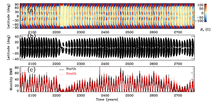
Figure 1.— Temporal variations of (a) the azimuthal-averaged surface radial field, (b) latitudes of BMRs, and (c) the monthly numbers of BMRs from Run A2.

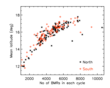
Figure 2.— Scatter plot between the mean latitudes of BMRs and the total BMR numbers both computed in each cycle. Red/black are obtained from northern/southern hemispheric cycles.

Our model produces the first BMR, when $\hat{B}(\theta,\phi)>B_{t}(\theta)$. Then after a time $dt$ since the previous BMR eruption, the model produces the next BMR only when two conditions, $\hat{B}(\theta,\phi)>B_{t}(\theta)$ and $dt\geq\Delta$ are satisfied. Here $\Delta$ follows a log-normal distribution that is obtained by fitting the time delay between the observed sunspots:

$$P(\Delta)=\frac{1}{\sigma_{\rm d}\Delta\sqrt{2\pi}}\exp\left[-\frac{(\ln\Delta-\mu_{\rm d})^{2}}{2\sigma_{\rm d}^{2}}\right],$$ (3)

where $\sigma_{\rm d}^{2}=(2/3)\left[\ln\tau_{\rm s}-\ln\tau_{\rm p}\right]$ and $\mu_{\rm d}=\sigma_{\rm d}^{2}+\ln\tau_{\rm p}$. In Sets B and B^′, we take $\tau_{\rm p}=0.8$ days and $\tau_{\rm s}=1.9$ days, as derived from the group sunspot data during solar maxima. However, in Sets A and A^′, we consider,

$$\tau_{\rm p}=\frac{2.2~{}\mathrm{days}}{1+(B_{b}^{N}/B_{\tau})^{2}}~{},\quad\tau_{\rm s}=\frac{20~{}\mathrm{days}}{1+(B_{b}^{N}/B_{\tau})^{2}}~{},$$ (4)

where $B_{b}^{N}$ is the azimuthal-averaged toroidal magnetic field in a thin layer from $r=0.715R_{\odot}$ to $0.73R_{\odot}$ around $15^{\circ}$ latitudes and $B_{\tau}=400$ G. Hence the delay distribution changes in response to the toroidal field at the base of the CZ to allow less frequent BMRs when the toroidal field is weak and vice versa. We note that the whole process is done independently in each hemisphere so that no hemispheric symmetry is imposed in the flux emergence.

Once the timing of eruption is decided, other properties of BMR on the surface are obtained from observations. The field strength of BMR is set to 3 kG, while the area is obtained by using the observed distribution of BMR flux (Muñoz-Jaramillo et al., 2015):

$$P(\Phi)=\Phi_{0}\frac{1}{\sigma_{\Phi}\Phi\sqrt{2\pi}}\exp\left[-\frac{(\ln\Phi-\mu_{\Phi})^{2}}{2\sigma_{\Phi}^{2}}\right],$$ (5)

with $\mu_{\Phi}=51.2$, and $\sigma_{\Phi}=0.77$. The factor $\Phi_{0}$ regulates the strength of the dynamo (or the dynamo number); see Table 1.

To emphasis our prescription, in Sets A and A^′, it is the BMR time delay part through which the toroidal field is linked to the BMRs.  The BMR spot flux is taken from Equation (5). However, in Sets B and B^′ the toroidal field is linked in a different way. As mentioned above, in these sets, the delay distribution is kept unchanged, but the (observed) BMR flux distribution is scaled linearly with the toroidal field at the base of the CZ.  Thus, in these sets, the BMR spot flux $\Phi_{s}=(\hat{B}(\theta_{s},\phi_{s},t)/B_{\rm sat})\Phi$, where ($\theta_{s},\phi_{s}$) is the location of the BMR, and $\Phi$ is obtained from Equation (5).

For the tilts of BMRs, we consider Joy’s law with a Gaussian scatter around it with a given $\sigma_{\delta}$ inferred from observations (Dasi-Espuig et al., 2010; Stenflo & Kosovichev, 2012; McClintock et al., 2014; Wang et al., 2015; Arlt et al., 2016; Jha et al., 2020). For further details of the model, readers are encouraged to go through Karak & Miesch (2017).

2. Results

In Table 1, we enlist some of the key parameters and results of our primary simulations. In Set A, Run A0 is subcritical, while all other Runs produce dynamo cycles. Runs A1–A4 produce a stable magnetic field. In Figure 1, we show the time evolutions of various quantities for about 700 years from Run A2. We observe that this simulation produces an overall stable magnetic field even without including any explicit nonlinear quenching. After continuing this simulation for 1545 years, we find that the magnetic field overall remains stable. Other than the stable magnetic field, the simulation produces most of the basic features of the solar cycle, namely, polarity reversals, dipole dominated field near minima, amplitude variation, north-south asymmetry, and mixed-polarity field. All Runs A1–A4 show these features. The variation in the magnetic field in these simulations is due to the scatter in BMR tilt and the randomness in BMR emergences. We note that in our modeled solar cycle, we do not observe the Gnevyshev-Ohl rule even when we include the tilt quenching in addition to the latitude quenching. Hence, the prediction of Jiang (2020) based on the SFT model does not hold in our dynamo model.

Another feature that we observe in this simulation is that the latitudinal extent of the BMRs in each cycle is not constant. As seen in Figure 1b, stronger cycles start producing BMRs at higher latitudes, while weaker ones produce BMRs at lower latitudes. This feature is nicely seen in Figure 2. It shows a positive trend between the mean latitude of BMRs and the total number of BMRs in each cycle, consistent with observations (Waldmeier, 1955; Solanki et al., 2008; Jiang et al., 2011; Mandal et al., 2017). It is this feature of our model, which gives rise to the latitudinal quenching and stabilizes the magnetic field growth.

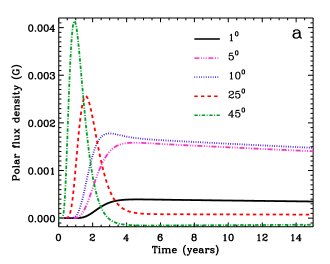
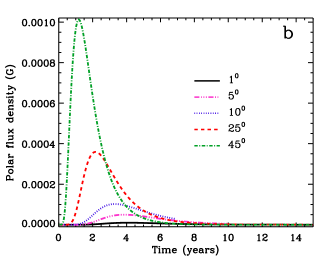
Figure 3.— Time evolution of the polar magnetic flux density averaged over $55^{\circ}$ to pole in the northern hemisphere. Solid, dash double-dot, dot, dash, and dash-dot lines correspond to simulations with BMR pair at $\pm 1^{\circ}$, $\pm 5^{\circ}$, $\pm 10^{\circ}$, $\pm 25^{\circ}$, and $\pm 45^{\circ}$ latitudes, respectively. (a) and (b) correspond to simulations with and without magnetic pumping, respectively.

To demonstrate how this is happening in our model, we make the following clean experiment. We perform four simulations by depositing two identical BMRs at latitudes: $\pm 1^{\circ}$, $\pm 5^{\circ}$, $\pm 10^{\circ}$, $\pm 25^{\circ}$, and $\pm 45^{\circ}$. We mean, at the beginning of each simulation, we deposit one BMR at a given latitude in the northern hemisphere and another one exactly at the same latitude in the southern hemisphere. The tilt is assigned by Joy’s law with no scatter around it. No other initial magnetic field is given. The time evolutions of the surface radial magnetic flux densities averaged over $55^{\circ}$ to the pole from these simulations are shown in Figure 3a. We observe that with the increase of BMR latitude, from $1^{\circ}$ to $10^{\circ}$, the polar flux increases (due to the increase of tilt). However, then with the increase of latitude, the polar flux rapidly decreases (due to less efficient cancellation of the opposite polarity flux at the equator). The BMR pair at $\pm 45^{\circ}$ gives even little negative polar flux. Thus in our dynamo simulation, the BMRs at higher latitudes give rise to less polar flux which is also true in the SFT model (Jiang et al., 2014).

This behavior does not hold entirely if we do not include the downward magnetic pumping in our model. As seen in Figure 3b, the polar field in the early phase from models without pumping behaves similarly to that from models with pumping. However, after a few years, the magnetic field decays quickly; Hazra et al. (2017) also found a similar behavior. This does not happen when there is pumping. It was already realized in previous studies that a magnetic pumping is needed to make the results of dynamo models consistent with SFT models and the observations (Cameron et al., 2012; Karak & Miesch, 2018).

Thus in our model, due to the inclusion of latitude-dependent threshold for BMR eruption (Equation (2)), when the toroidal magnetic field tries to grow in one cycle, the mean latitude of BMRs increases. As seen above, the BMRs at higher latitudes are far less efficient in generating poloidal field. This effect halts the growth of the magnetic field in our dynamo model.

As expected, when we remove the latitude-dependent threshold for BMR eruption in Set A^′, the dynamo cannot produce a stable magnetic field. This happened in Runs A^′1–A^′2. However, Run A^′2^∗, which is the same as Run A^′2 except a tilt quenching of the form $1/[1+(\hat{B}(\theta,\phi,t)/B_{\rm sat})^{2}]$ (where the saturation field $B_{\rm sat}=1\times 10^{5}$ G) is included, also fails to produce a stable magnetic field.

We have made several simulations by changing some parameters in the model. Run A3 is the case in which we have switched off the scatter in the BMR tilt around Joy’s law. We again find a stable solution. However, when $\Phi_{0}$ is sufficiently above the critical value needed for the dynamo transition, the model fails to produce a stable magnetic field. This is because of an opposing effect arose at large $\Phi_{0}$. When $\Phi_{0}$ is large, the BMR flux distribution (Equation (5)) is moved to a higher side. Thus the individual BMR gets more flux, which consequently generates a large poloidal flux. When this effect dominates over the reduction of poloidal flux by the latitudinal quenching, the model fails to provide a stable magnetic field. This happened in Run A5. Interestingly, in this run when we include a tilt quenching, it also fails to produce a stable magnetic field (Run A5^∗ in Table 1). Thus when the dynamo is too much supercritical, both the latitudinal and tilt quenchings, even operating together, fail to produce a stable magnetic field in Set A.

We note that in Sets A and A^′, when a model fails to limit the magnetic field growth at large $\Phi_{0}$, the magnetic field cannot grow indefinitely because of a numerical means. At large $\Phi_{0}$, the strong magnetic field makes the delay distribution for BMR eruptions narrow (equations (3) and (4)). Meaning, $\Delta$ is less. However, the actual $\Delta$ cannot be less than the time step of numerical integration of our differential equations. Hence, when the magnetic field is sufficiently high to make the delay less than or equal to the numerical time step, the growth of the magnetic field is artificially halted. However, this does not happen when $\Phi_{0}$ is not too much larger than the critical value for the dynamo transition. Thus in Runs A1–A3 the delay never became less than the numerical time step and the magnetic field growth is limited by the latitudinal quenching alone.

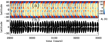
Figure 4.— The same as Figure 1 but obtained from Run B2.

This issue is not there in Set B because in this case, the delay distribution is kept at the observed value. Again in Runs B1–B4, we find a stable solution without including any nonlinearly in the model. Only the latitudinal effect of BMR eruption as discussed above is responsible for the stability of the magnetic field. Time evolutions of various quantities from Run B2 are presented in Figure 4. Again we observe a stable magnetic field and the basic features of the observed solar magnetic field. However, when we make the dynamo too strong by increasing $\Phi_{0}$ much above the critical value, we examine that the latitudinal quenching is not able to halt the growth of the magnetic field. This is seen in Run B5. Nevertheless, when we include the tilt quenching, the model manages to halt the magnetic field growth in this case; see Run B5^∗.

Based on the physics presented in Figure 3, it is expected that if we exclude the magnetic pumping, the model fails to produce a stable magnetic cycle through the latitudinal quenching alone. To demonstrate this, we show a few additional simulations Runs B^′0–B^′3. We note that when we put pumping to zero, the dynamo model fails to produce growing field unless we reduce the diffusivity in the CZ considerably or increase $\Phi_{0}$ to a very high value. It is already known that the flux transport dynamo cannot produce 11-year solar cycle at high diffusivity ($\sim 10^{12}$ cm² s^-1) (Karak & Choudhuri, 2012). Thus we reduce the diffusivity in this runs by taking $\eta_{\mathrm{CZ}}=5\times 10^{10}$ cm² s^-1, and $\eta_{\mathrm{S}}=1\times 10^{12}$ cm² s^-1. Other than this change in the diffusivity, the B^′ Set in Table 1 is the same as Set B. From Table 1 we observe that when $\Phi_{0}$ is above a certain value, the model produces growing field but no stable magnetic cycle.

3. Summary and Conclusions

We have demonstrated the saturation of the magnetic field in the kinematic Babcock–Leighton type flux transport dynamo models through the latitudinal quenching as proposed by Jiang (2020). It is based on the observed fact that the stronger cycles produce sunspots and BMRs at higher latitudes than the weaker ones. The BMRs at higher latitudes are less efficient in producing the poloidal field. This effect alone halts the growth of the magnetic field in our dynamo model. However, when the dynamo is too much supercritical (much above the dynamo transition), the latitudinal quenching cannot limit the growth of the magnetic field in our model. Incidentally, there are some indications that the solar dynamo is not too much supercritical (Metcalfe et al., 2016; Kitchatinov & Nepomnyashchikh, 2017). Thus we conclude that the latitudinal variation of BMR is a potential candidate for the saturation of the solar dynamo.

References

- Arlt et al. (2016) Arlt, R., Senthamizh Pavai, V., Schmiel, C., & Spada, F. 2016, A&A, 595, A104
- Baumann et al. (2004) Baumann, I., Schmitt, D., Schüssler, M., & Solanki, S. K. 2004, A&A, 426, 1075
- Cameron & Schüssler (2015) Cameron, R., & Schüssler, M. 2015, Science, 347, 1333
- Cameron et al. (2017) Cameron, R. H., Dikpati, M., & Brandenburg, A. 2017, Space Sci. Rev., 210, 367
- Cameron et al. (2012) Cameron, R. H., Schmitt, D., Jiang, J., & Işık, E. 2012, A&A, 542, A127
- Cameron & Schüssler (2016) Cameron, R. H., & Schüssler, M. 2016, A&A, 591, A46
- Cameron & Schüssler (2017) —. 2017, ApJ, 843, 111
- Charbonneau (2010) Charbonneau, P. 2010, Liv. Rev. Sol. Phys., 7, 3
- Choudhuri (2014) Choudhuri, A. R. 2014, Indian Journal of Physics, 88, 877
- Choudhuri et al. (2007) Choudhuri, A. R., Chatterjee, P., & Jiang, J. 2007, Physical Review Letters, 98, 131103
- Choudhuri & Karak (2012) Choudhuri, A. R., & Karak, B. B. 2012, Phys. Rev. Lett., 109, 171103
- Dasi-Espuig et al. (2010) Dasi-Espuig, M., Solanki, S. K., Krivova, N. A., Cameron, R., & Peñuela, T. 2010, A&A, 518, A7
- Dikpati & Charbonneau (1999) Dikpati, M., & Charbonneau, P. 1999, ApJ, 518, 508
- Dikpati et al. (2004) Dikpati, M., de Toma, G., Gilman, P. A., Arge, C. N., & White, O. R. 2004, ApJ, 601, 1136
- Dikpati et al. (2009) Dikpati, M., Gilman, P. A., Cally, P. S., & Miesch, M. S. 2009, ApJ, 692, 1421
- Hazra et al. (2017) Hazra, G., Choudhuri, A. R., & Miesch, M. S. 2017, ApJ, 835, 39
- Howe (2009) Howe, R. 2009, Living Reviews in Solar Physics, 6, 1
- Jha et al. (2020) Jha, B. K., Karak, B. B., Mandal, S., & Banerjee, D. 2020, ApJ, 889, L19
- Jiang (2020) Jiang, J. 2020, ApJ in press, arXiv: 2007.07069
- Jiang et al. (2011) Jiang, J., Cameron, R. H., Schmitt, D., & Schüssler, M. 2011, A&A, 528, A82
- Jiang et al. (2014) Jiang, J., Cameron, R. H., & Schüssler, M. 2014, ApJ, 791, 5
- Karak (2010) Karak, B. B. 2010, ApJ, 724, 1021
- Karak & Cameron (2016) Karak, B. B., & Cameron, R. 2016, ApJ, 832, 94
- Karak & Choudhuri (2011) Karak, B. B., & Choudhuri, A. R. 2011, MNRAS, 410, 1503
- Karak & Choudhuri (2012) —. 2012, Sol. Phys., 278, 137
- Karak et al. (2018) Karak, B. B., Mandal, S., & Banerjee, D. 2018, ApJ, 866, 17
- Karak & Miesch (2017) Karak, B. B., & Miesch, M. 2017, ApJ, 847, 69
- Karak & Miesch (2018) —. 2018, ApJ, 860, L26
- Kitchatinov & Nepomnyashchikh (2017) Kitchatinov, L., & Nepomnyashchikh, A. 2017, MNRAS, 470, 3124
- Kitchatinov (2020) Kitchatinov, L. L. 2020, ApJ, 893, 131
- Kitchatinov & Olemskoy (2011a) Kitchatinov, L. L., & Olemskoy, S. V. 2011a, Astronomische Nachrichten, 332, 496
- Kitchatinov & Olemskoy (2011b) —. 2011b, Astronomy Letters, 37, 656
- Lemerle & Charbonneau (2017) Lemerle, A., & Charbonneau, P. 2017, ApJ, 834, 133
- Mandal et al. (2017) Mandal, S., Karak, B. B., & Banerjee, D. 2017, ApJ, 851, 70
- McClintock et al. (2014) McClintock, B. H., Norton, A. A., & Li, J. 2014, ApJ, 797, 130
- Metcalfe et al. (2016) Metcalfe, T. S., Egeland, R., & van Saders, J. 2016, ApJ, 826, L2
- Miesch & Dikpati (2014) Miesch, M. S., & Dikpati, M. 2014, ApJ, 785, L8
- Miesch & Teweldebirhan (2016) Miesch, M. S., & Teweldebirhan, K. 2016, Space Sci. Rev.
- Muñoz-Jaramillo et al. (2013) Muñoz-Jaramillo, A., Dasi-Espuig, M., Balmaceda, L. A., & DeLuca, E. E. 2013, ApJ, 767, L25
- Muñoz-Jaramillo et al. (2015) Muñoz-Jaramillo, A., et al. 2015, ApJ, 800, 48
- Olemskoy & Kitchatinov (2013) Olemskoy, S. V., & Kitchatinov, L. L. 2013, ApJ, 777, 71
- Parfrey & Menou (2007) Parfrey, K. P., & Menou, K. 2007, ApJ, 667, L207
- Priyal et al. (2014) Priyal, M., Banerjee, D., Karak, B. B., Muñoz-Jaramillo, A., Ravindra, B., Choudhuri, A. R., & Singh, J. 2014, ApJ, 793, L4
- Solanki et al. (2008) Solanki, S. K., Wenzler, T., & Schmitt, D. 2008, A&A, 483, 623
- Stenflo & Kosovichev (2012) Stenflo, J. O., & Kosovichev, A. G. 2012, ApJ, 745, 129
- Upton & Hathaway (2014) Upton, L., & Hathaway, D. H. 2014, ApJ, 780, 5
- Usoskin (2013) Usoskin, I. G. 2013, Living Reviews in Solar Physics, 10, 1
- Waldmeier (1955) Waldmeier, M. 1955, Ergebnisse und Probleme der Sonnenforschung.
- Wang et al. (2015) Wang, Y.-M., Colaninno, R. C., Baranyi, T., & Li, J. 2015, ApJ, 798, 50